8 Advection equations and the art of numerical modeling

More documents

Recommendations

Info

Numerische Methoden 1 – B.J.P. Kaus% advection_central_1D%clear allnx = 201;W = 40; % width of domainVel = -4; % velocitysigma = 1;Ampl = 2;nt = 500; % number of timestepsdt = 1e-2;dx = W/(nx-1);x = 0:dx:W;% Initial gaussian T-profilexc = 20;T = Ampl*exp(-(x-xc).^2/sigma^2);% VelocityVx = ones(1,nx)*Vel;% Central finite difference discretizationfor itime=1:nt% central fin. difffor ix=2:nx-1Tnew(ix) = ??endTnew(1) = T(1);Tnew(nx) = T(nx);T = Tnew;time = itime*dt;% Analytical solution for this caseT_anal = Ampl*exp(-(x-xc-time*Vel).^2/sigma^2);figure(1),clf, plot(x,T,x,T_anal),drawnowendlegend(’Numerical’,’Analytical’)Figure 2: MATLAB script to be used with exercise 1.8.1 FTCS methodIn a 1-D case the simplest way to discretize equation 3 is by employing a central finite difference scheme(also called the forward-time, central space or FTCS scheme):T n+1i− Tin∆t= −v x,iT n i+1 − T n i−12∆x(5)8.1.1 Exercise 1• Program the FTCS method in the code of figure 2 and watch what happens. Change the sign ofthe velocity. Change the timestep and gridspacing and compute the nondimensional parameterα = |v x |∆t/∆x. When do unstable results occur?As you saw from the exercise, the FTCS method does not work... In fact it is a nice example of ascheme that looks nice (and logical!) on paper, but sucks [you can actually mathematically prove thisby a socalled von Neuman stability analysis, if you’re interested you should read chapter 5 of MarcSpiegelman’s script on the course webpage; it’s related to the fact that this scheme produces antidiffusion,which is numerically instable].8.2 Lax methodin the time-Some day, long ago, there was a guy called Lax and he thought: well let’s replace the Tinderivative of equation 5 with (Ti+1 n + T i−1 n )/2. The resulting equation isT n+1i − (Ti+1 n + T i−1 n )/2 Ti+1 n = −v − T i−1nx,i∆t2∆x(6)2
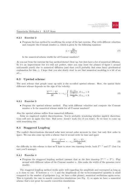
Numerische Methoden 1 – B.J.P. Kaus8.2.1 Exercise 2• Program the Lax method by modifying the script of the last exercise. Play with different velocitiesand compute the Courant number α, which is given by the following equation:α =∆x∆t|v x |(7)Is the numerical scheme stable for all Courant numbers?As you saw from the exercise the Lax method doesn’t blow up, but does have a lot of numerical diffusion.So it’s an improvement but it’s still not perfect, since you may loose the plumes of figure 1 aroundmid-mantle purely due to numerical diffusion (and than you’ll probably find some fancy geochemicalexplanation for this...). I hope that you also slowly start to see that numerical modeling is a bit of anart...8.3 Upwind schemeThe next scheme that people came up with is the so-called upwind scheme.difference scheme depends on the sign of the velocity:Here, the spatial finiteT n+1i− Tin∆t= −v x,i{ Tni −T n i−1∆x, if v x,i > 0T n i+1 −T n i∆x, if v x,i < 0(8)8.3.1 Exercise 3• Program the upwind scheme method. Play with different velocities and compute the Courantnumber α Is the numerical scheme stable for all Courant numbers?Also the upwind scheme suffers from numerical diffusion.Sofar we employed explicit discretizations. You’re probably wondering whether implicit discretizationswill save us again this time. Bad news: doesn’t work (try if you want). So we have to come upwith something else.8.4 Staggered LeapfrogThe explicit discretizations discussed sofar were second order accurate in time, but only first order inspace. We can also come up with a scheme that is second order in time and spaceT n+1i− T n−12∆t= −v x,iT n i+1 − T n i−12∆xthe difficulty in this scheme is that we’ll have to store two timestep levels: both T n−1 and T n (but i’msure you’ll manage).(9)8.4.1 Exercise 4• Program the staggered leapfrog method (assume that at the first timestep T n−1 = T n ). Playaround with different values of the Courant number α. Also make the width of the gaussian curvesmaller.The staggered leapfrog method works quite well regarding the amplitude and wavespeed as long asα is close to one. If however α
Page 1: Numerische Methoden 1 - B.J.P. Kaus
Page 5: Numerische Methoden 1 - B.J.P. Kaus

8 Advection equations and the art of numerical modeling

You also want an ePaper? Increase the reach of your titles

Delete template?

Save as template?