Subdivision Schemes and Attractors - CiteSeerX

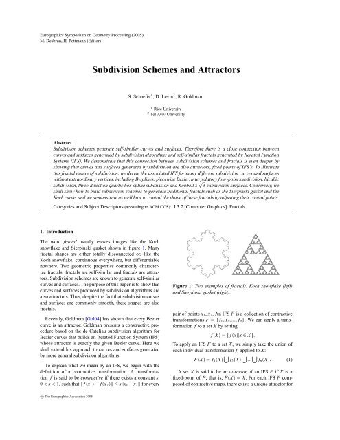
Eurographics Symposium on Geometry Processing (2005)M. Desbrun, H. Pottmann (Editors)Subdivision Schemes and AttractorsS. Schaefer 1 , D. Levin 2 , R. Goldman 11 Rice University2 Tel Aviv UniversityAbstractSubdivision schemes generate self-similar curves and surfaces. Therefore there is a close connection betweencurves and surfaces generated by subdivision algorithms and self-similar fractals generated by Iterated FunctionSystems (IFS). We demonstrate that this connection between subdivision schemes and fractals is even deeper byshowing that curves and surfaces generated by subdivision are also attractors, fixed points of IFS’s. To illustratethis fractal nature of subdivision, we derive the associated IFS for many different subdivision curves and surfaceswithout extraordinary vertices, including B-splines, piecewise Bezier, interpolatory four-point subdivision, bicubicsubdivision, three-direction quartic box-spline subdivision and Kobbelt’s √ 3-subdivision surfaces. Conversely, weshall show how to build subdivision schemes to generate traditional fractals such as the Sierpinski gasket and theKoch curve, and we demonstrate as well how to control the shape of these fractals by adjusting their control points.Categories and Subject Descriptors (according to ACM CCS): I.3.7 [Computer Graphics]: Fractals1. IntroductionThe word fractal usually evokes images like the Kochsnowflake and Sierpinski gasket shown in figure 1. Manyfractal shapes are either totally disconnected or, like theKoch snowflake, continuous everywhere, but differentiablenowhere. Two geometric properties commonly characterizefractals: fractals are self-similar and fractals are attractors.Subdivision schemes are known to generate self-similarcurves and surfaces. The purpose of this paper is to show thatcurves and surfaces produced by subdivision algorithms arealso attractors. Thus, despite the fact that subdivision curvesand surfaces are commonly smooth, these shapes are alsofractals.Recently, Goldman [Gol04] has shown that every Beziercurve is an attractor. Goldman presents a constructive procedurebased on the de Cateljau subdivision algorithm forBezier curves that builds an Iterated Function System (IFS)whose attractor is exactly the given Bezier curve. Here weshall extend his approach to curves and surfaces generatedby more general subdivision algorithms.To explain what we mean by an IFS, we begin with thedefinition of a contractive transformation. A transformationf is said to be contractive if there exists a constant s,0 < s < 1, such that ‖ f(x 1 ) − f(x 2 )‖ ≤ s‖x 1 − x 2 ‖ for everyFigure 1: Two examples of fractals. Koch snowflake (left)and Sierpinski gasket (right).pair of points x 1 , x 2 . An IFS F is a collection of contractivetransformations F = { f 1 , f 2 ,..., f n}. We can apply a transformationf to a set X by settingf(X) = { f(x)|x ∈ X}.To apply an IFS F to a set X, we simply take the union ofeach individual transformation f i applied to X:F(X) = f 1 (X) [ f 2 (X) [ ... [ f n(X). (1)A set X is said to be an attractor of an IFS F if X is afixed-point of F; that is, F(X) = X. For each IFS F composedof contractive maps, there exists a unique attractor forc○ The Eurographics Association 2005.

S. Schaefer, D. Levin, R. Goldman / Subdivision Schemes and AttractorsFigure 2: A control polygon converging to a limit curve using uniform cubic B-spline subdivision with p 0 , p 1 , p 2 , p 3 and p ∞shown (Top). Starting with an arbitrary point and iterating the B-spline IFS also converges to the same curve (Bottom).F, which we denote by F ∞ [Bar93]. To generate F ∞ , wecan start with any compact set X 0 and iterate X i+1 = F(X i ).Remarkably, any compact set X 0 will converge to F ∞ underiteration. Both the Koch snowflake and the Sierpinski triangleare attractors; that is, they are each fixed points of anIFS. Therefore, attractors are often synonymous with fractals[Bar93].While Goldman concentrated on generating IFS’s forBezier curves, we are interested in curves generated by moregeneral subdivision procedures such as B-splines. B-splinescurves of degree n are curves specified over a set of knotst 0 ...t m, where the curve in between t i and t i+1 is a Beziercurve of degree n. If the knots are distinct, these curvesare C n−1 everywhere and contain a discontinuity in the n thderivative at each of the knots t i .Since B-splines are composed of piecewise Bezier curves,each of which is an attractor, it is natural to wonder whetherB-splines are also attractors. However, constructing an IFSwhose attractor is the union of two or more attractors isnot so simple. Moreover, there exists arguments to suggestthat an IFS for B-splines does not exist. Fractals are selfsimilar,composed of smaller copies of themselves. For example,the Sierpinski gasket in figure 1 is composed ofthree smaller Sierpinski gaskets. A B-spline composed oftwo Bezier curves is a piecewise n th degree polynomial thatcontains a discontinuity in the n th derivative at the centralknot. The self-similarity of such a curve is not readilyapparent, since the discontinuity must vanish on the selfsimilarpieces. Nevertheless, despite this apparent obstruction,in section 2.1 we shall show how to construct an IFSfor uniform B-splines as well as for more general subdivisionschemes.ContributionsInspired by Goldman’s work, we propose to bridge thegap between subdivision curves and surfaces and the worldof fractals by showing that the shapes generated by subdivisionare themselves attractors of an IFS. For any splinecurve with uniform knots, we shall present a constructivemethod for generating an IFS whose attractor is the givenspline. Furthermore, we will show how any curve generatedby an arbitrary stationary subdivision scheme can be representedby an IFS. We also examine subdivision surfaces inthe ordinary case (no extraordinary vertices) and show howseveral surface subdivision schemes, including rectangularmethods like bicubic spline subdivision [CC78] and trianglemethods such as three-direction quartic box-spline subdivision[Loo87] and √ 3-subdivision [Kob00], can also berepresented using an IFS. Finally, we also consider the conversequestion: can traditional fractals be generated throughsubdivision using a set of control points? We provide a generalparadigm for introducing control points and subdivisionrules for arbitrary fractals generated by an IFS consistingof affine transformations. We then illustrate our approachby introducing control points and subdivision rules for theSierpinski gasket and the Koch curve. We also show how toadjust the shape of these fractals in an intuitive fashion bymoving their control points.Previous WorkIn addition to Goldman’s work on IFS’s for Beziercurves [Gol04], Prautzsch and Micchelli [PM87] studyfractal-like curves generated by subdivision. However, thecurves they generate are not smooth. Kocić [Koc96] alsoconsiders Bernstein polynomials as fractals.Kocić and Simoncelli [KS98] introduce Affine IteratedFunction Systems, which use barycentric rather than rectangularor homogeneous coordinates to generate fractalshapes. The purpose of their method is to extend the definitionof an IFS to include control points in order to governthe shape of the attractor. In contrast, we show how traditionalfractals can be generated by subdivision rules. Kocićand Simoncelli also anticipate some of our work on fractalcurves by constructing IFS matrices for uniform B-splines.However, they provide no general insight to show that an arbitrarybinary subdivision scheme is necessarily an attractor;nor do they consider subdivision surfaces.c○ The Eurographics Association 2005.

S. Schaefer, D. Levin, R. Goldman / Subdivision Schemes and AttractorsFigure 3: Subdivision of a cubic B-spline curve with tripled knots at the end points to force interpolation (Top). Starting with atriangle and iterating the associated B-spline IFS generates the same curve despite self-intersection (Bottom).2. CurvesWe begin by presenting a method for constructing an IFSfor any curve defined by an arbitrary, stationary subdivisionscheme. We show that the attractor of this IFS is exactly thecurve defined by the subdivision scheme and a given set ofcontrol points, independent of the starting set X 0 used forthe IFS. Next, we illustrate our construction by generatingIFS’s for uniform cubic B-spline curves. We then extend thismethod to show that we can handle end-point conditions,where the knot spacing is non-uniform. We also show thatthis method can generate an IFS for other types of subdivisioncurves such as non-polynomial curves produced by thefour-point subdivision scheme [DGL87].Subdivision schemes for curves are defined by a set ofrules that take in a set of control points p k as input and producea new, refined set of control points p k+1 as output. Subdivisionis a recursive procedure and repeating this processyields a limit curve p ∞ . For our purposes, we consider binarysubdivision schemes for curves with two sets of rulesof the formp k+12i = ∑ j α j p k j+ip k+12i+1 = ∑ j β j p k j+iwhere α j and β j are numerical coefficients and ∑α j =∑β j = 1. For instance, uniform cubic B-splines have an associatedsubdivision scheme with rules given in equation 4.Notice that these binary subdivision rules may also be writtenin matrix form as⎛S =⎜⎝... ... ... ... ... ... ...... β 0 β 1 β 2 β 3 β 4 ...... α −1 α 0 α 1 α 2 α 3 ...... β −1 β 0 β 1 β 2 β 3 ...... α −2 α −1 α 0 α 1 α 2 ...... β −2 β −1 β 0 β 1 β 2 ...... α −3 α −2 α −1 α 0 α 1 ...... β −3 β −2 β −1 β 0 β 1 ...... ... ... ... ... ... ...⎞.⎟⎠Let P be a matrix of control points for p 0 , where the i throw of P contains the control point p 0 i . To build an IFS correspondingto the curve with control points p 0 and subdivisionmatrix S, we break the matrix S apart into multiplesquare matrices S 1 ,S 2 ,...,S n such that applying all productsof S i of length k to the control points P converges to p ∞ ask approaches ∞. Note that, in order to form square matrices,some of the rows of the matrices S i may overlap (forexample, see the B-spline matrices in section 2.1). This decompositionof the matrix S into the matrices S i is the sameas the decomposition used in the joint spectral radius calculationintroduced by Levin and Levin [LL03] to study thesmoothness properties of various subdivision schemes. Nowconstruct an IFS by lettingf i (X) = XP −1 S i P. (2)Notice that P may not actually be invertible or even asquare matrix. To construct a form of P suitable for equation2, we shall lift the points in P to a higher dimension. Tomake the matrix P square and invertible, we concatenate thecolumns of P with rows from an identity matrix to make Psize n × n − 1; then we change the coordinates into homogeneousform by adding a column of ones to P, making P asquare matrix. This new square matrix is invertible as longas the original control points form an affine basis (i.e., thevertices do not all lie on a straight line).Now if we choose our starting set X 0 to be P, then applyingequation 1 simulates subdivision and generates exactlythe curve p ∞ . Since the fractal generated by an IFS is uniqueif the f i are contractive maps, iteration on any compact setX 0 would yield the same fractal. Therefore, the attractor ofthis IFS is exactly the limit curve p ∞ as long as the f i arecontractive maps.This independence of the starting set X 0 is somewhatcounter-intuitive. Certainly if we begin with the controlpoints P, this process should converge to the limit curve p ∞ .However, uniqueness asserts that iterating on any compactstarting set will converge to the exact same fractal. Figures 2,5 and 3 show examples that start the iteration with a singlepoint, a line and even a triangle. In these examples, iterationconverges to the attractor regardless of the initial shape.c○ The Eurographics Association 2005.

S. Schaefer, D. Levin, R. Goldman / Subdivision Schemes and AttractorsFigure 5: Subdivision using the four-point rule (Top). Starting with a line and iterating the IFS also converges to the samecurve (Bottom).S 2 that correspond to inserting knots to form the knot sequence{0,0,0, 1 2 ,1,1,1, 3 2 ,2,2,2}.⎛⎞1 0 0 0 01 12 2 0 0 0S 1 =3 1⎜ 0 4 4 0 0⎟⎝ 3 1 10 8 2 8 0 ⎠1 1 10 4 2 4 0⎛ 1 1 1 ⎞0 4 2 4 01 1 3 0 8 2 8 0S 2 =1 3⎜ 0 0 4 4 0⎟⎝1 10 0 0 ⎠2 20 0 0 0 1Figure 3 shows a triangle converging under the action ofthis IFS to a cubic B-spline with interpolating endpoint conditions.Similar subdivision algorithms exist for any knotsequence where knot insertion generates a self-similar sequenceof knots.2.2. Bezier CurvesThough Goldman showed how a single Bezier curve couldbe generated from an IFS, he did not discuss how to build anIFS for multiple Bezier curves that meet with various levelsof smoothness. Using our technique, we can construct a singleIFS whose attractor is two disjoint Bezier curves. Sinceeach Bezier curve can be represented by an IFS, our methodgenerates a single IFS whose attractor is the union of theattractors from the two individual IFS’s.For a single quadratic Bezier curve, the two subdivisionmatrices for the corresponding IFS are⎛1 0 0⎞141214S 1 = ⎝ 1212 0 ⎠⎛ 1 1 1 ⎞4 2 4S 2 = ⎝ 1 10 2 2⎠.0 0 1Given two quadratic Bezier curves with control points P, Qwritten as rows in homogeneous form, we construct the IFSfor the union of the two Bezier curves using block matricesas( P −1 )Sf 1 (X) = X 1 P 00 Q −1 S 1 Q( P −1 Sf 2 (X) = X 2 P 00 Q −1 S 2 Q).While similar to the curve matrices developed in section2.1, there is a complication that arises when using thisunion technique. Each matrix S 1 , S 2 contains an eigenvalueof 1 that corresponds to the homogeneous component in thecontrol points. However, in block form, the new matrix containstwo eigenvalues of 1 because there are now two homogeneouscomponents. Therefore, to make sure the f i arestill contractive maps, we require that the starting set X 0 forequation 1 contain 1’s in each of the two homogeneous components.Figure 4 shows an attractor consisting of two Beziercurves generated using this technique. For the starting setX 0 , we used a single point of the form {x 1 ,y 1 ,1,x 2 ,y 2 ,1}. Torender the fractal, we draw the points {x 1 ,y 1 } and {x 2 ,y 2 }.While this method generates an IFS whose attractor is theunion of two Bezier curves, a B-spline curve is composed ofmultiple Bezier curves that meet with C n−1 continuity for adegree n curve. Therefore, for Bezier curves meeting withC n−1 smoothness, we get similar results in a more compactform using the B-spline matrices from section 2.1. However,the technique that we present here is general enough to constructan IFS whose attractor is the union of the attractors ofany two IFS’s whose transformations consist of matrix multiplication.2.3. Four-Point SubdivisionUntil now, all of our examples using this IFS constructionhave converged to curves that are piecewise polynomial.However, there is nothing special about polynomials and ourmethod can operate on arbitrary subdivision schemes. Forinstance, the four-point subdivision scheme is an interpolac○The Eurographics Association 2005.

S. Schaefer, D. Levin, R. Goldman / Subdivision Schemes and AttractorsFigure 6: Subdivision for a bicubic spline surface (Top). Generating the same surface using an IFS (Bottom).Figure 7: Three-direction quartic box-spline subdivision for a hexagonal patch (Top). Starting with a single triangle anditerating the IFS converges to the same surface (Bottom).tory scheme whose rules arep k+12i = p k ip k+12i+1 = −116 pk i−1 + 916 pk i + 916 pk i+1 − 116 pk i+2 .This subdivision scheme can reproduce cubic polynomials,though in general the four-point method generates smoothcurves that are not polynomial. Nevertheless, we can stillconstruct an IFS that converges to these curves. Below arethe subdivision matrices S 1 and S 2 used to construct this IFS.⎛S 1 =⎜⎝⎞0 1 0 0 0 0 0−1 9 9 −116 16 16 16 0 0 00 0 1 0 0 0 0−1 9 9 −10 16 16 16 16 0 00 0 0 1 0 0 0⎟−1 9 9 −10 0 16 16 16 16 0 ⎠0 0 0 0 1 0 0⎛⎞0 0 1 0 0 0 0−1 9 9 −10 16 16 16 16 0 00 0 0 1 0 0 0S 2 =−1 9 9 −10 0 16 16 16 16 0⎜ 0 0 0 0 1 0 0⎟⎝−1 9 9 −10 0 0⎠16 16 16 160 0 0 0 0 1 0Figure 5 depicts the fractal process starting with a line segment,which converges to the curve defined by this subdivisionscheme.3. SurfacesWhile the IFS construction in section 2 is specific to curves,the concepts are general enough to apply as well to subdivisionsurfaces. In this section, we show several examplesof IFS’s whose attractors are surfaces defined via uniformsubdivision. Though it is straightforward to extend the curvec○ The Eurographics Association 2005.

S. Schaefer, D. Levin, R. Goldman / Subdivision Schemes and AttractorsFigure 8: Kobbelt’s √ 3-subdivision for a hexagonal surface (Top). The same surface generated using an IFS (Bottom).methods from section 2 to tensor product surfaces, it maynot be immediately apparent that other subdivision schemessuch as Kobbelt’s √ 3-subdivision can also be generatingfrom an IFS.Similar to the curve case, we begin by constructing asubdivision matrix S that encodes the rules for subdividinga control polyhedron. Next, we separate this matrix intosquare matrices S i such that taking all possible combinationof these matrices of length k converges to the subdivisionsurface as k approaches ∞. Unfortunately, the subdivisionmatrices used to generate these surfaces are too large to includein the body of this paper. However, we have placed aMathematica notebook online at http://www.cs.rice.edu/ sschaefe/splineifs.nb,which includes our implementation ofthe IFS’s used for all the curves and surfaces in this paper.be used to generate an IFS. Figure 7 shows a hexagonal surfacecreated from a hexagonal grid of control points.Like many fractals, there is more than one way to writedown the transformations that generate this attractor. Eventhough this subdivision scheme is triangle-based, we couldhave split S into four matrices instead of the six we used infigure 7. However, the attractor in that case would look rectangularand similar to that of figure [CC78]. We chose sixmatrices in this case to create an attractor with a hexagonalshape to distinguish this attractor from the tensor productscheme in section 3.1.3.1. Bicubic Spline SubdivisionIn the uniform case, Catmull-Clark subdivision [CC78] operateson quadrilateral polygons and generates a tensor productscheme for uniform cubic B-splines. Since we can representa cubic B-spline as an IFS, we can also represent thissurface subdivision scheme as an IFS. For the surface IFS,we have four subdivision matrices instead of the two matricesfrom the curve examples in section 2.1. Figure 6 illustratesa bi-cubic patch constructed from a 4 × 4 grid ofcontrol points using this subdivision scheme. Starting witha single triangle, we apply the fractal process using the IFSwe have constructed and generate the same bi-cubic patch.3.2. Three-Direction Quartic Box-SplinesThree-direction quartic box-splines correspond to Loop subdivision[Loo87] in the uniform case. The surfaces that thisscheme takes as input are composed of triangles. In contrastto bicubic subdivision in section 3.1, this scheme cannot bewritten as a tensor product; however, this scheme may stillFigure 9: Three-direction quartic box-spline surface generatedby an IFS with six transformations (Left). The sameIFS with two of the six transformations removed creates afractal-like surface, which is a subset of the original surface(Right).3.3. Kobbelt’s √ 3-subdivision√Finally, surfaces generated by Kobbelt’s 3-subdivision [Kob00] can also be represented by an IFS. Likequartic box-spline subdivision in section 3.2, this schemeoperates on meshes of triangles. However, two rounds ofsubdivision using this scheme correspond to a ternary splitof the triangle polygons (hence the name √ 3-subdivision),whereas three-direction quartic box-spline subdivisionperforms a binary split at each level of subdivision.c○ The Eurographics Association 2005.

S. Schaefer, D. Levin, R. Goldman / Subdivision Schemes and AttractorsFigure 10: Applying the standard IFS for the Koch curve to a control polygon produces the fractal (Top). Starting with adifferent control polygon and applying the standard IFS still converges to the same fractal (Middle). With subdivision, movinga control point changes the shape of the Koch curve (Bottom).Though √ 3-subdivision is a somewhat exotic subdivisionscheme, the rules as well as the structure of the control pointsbehave in a self-similar fashion, which allows us to constructthe subdivision matrices necessary to build an IFS for thesesurfaces. Figure 8 (top) contains a surface generated throughuniform √ 3-subdivision on polygons. On the bottom of thefigure, we use the associated IFS to recover the same surfacestarting from a single triangle.The surfaces generated in this section are developedthrough an IFS; however, they certainly do not resemblefractal shapes such as the Sierpinski gasket from figure 1.Nevertheless, we can observe their underlying fractal structureby the following device. If F is an IFS and G ⊂ F, thefractal generated by G is a subset of the fractal generatedby F - that is, if G ⊂ F, then G ∞ ⊆ F ∞ . Thus if we wereto omit some of the matrices from an IFS that generates asubdivision surface, we would generate a fractal on the surface.Figure 9 shows a picture of the three-direction quarticbox-spline subdivision surface from figure 7 and a subset ofthe same surface generated by an IFS with two of the sixtransformations omitted. The resulting fractal surface verymuch resembles a Sierpinski gasket, but all of the points lieon the subdivision surface. This figure illustrates the underlyingfractal structure of these subdivision surfaces.strategy is to build the control points into the very fabric ofthe iterated function system of the fractal. The advantage ofthis control point representation for fractals is that controlpoints provide much finer control over the shape of a fractalthan standard IFS’s.Given an IFS defined by a set of affine transformationsF = { f 1 ,... f n}, we construct a subdivision scheme bychoosing a set of control points P = {P 1 ...P m}. These controlpoints may be any points in space. However, for manyfractals such as the Koch curve there are natural choices forthe control points (see figure 10).To build the subdivision rules for our fractal, we apply Fto P. For each vertex p j in f i (P), we represent p j as an affinecombination of the original control points P:p j = Σ k α j,k P k . (5)We construct the subdivision matrix S i corresponding to thetransformation f i by setting the j,k entry of S i to α j,k . Thesubdivision matrix S for this fractal is then simply the concatenationof the S i . Notice that the decomposition in equation5 does not yield a unique set of weights α j,k . In fact,many different choices for the weights are possible becausethe problem is underdetermined.4. Fractals with Control PointsSubdivision schemes have advantages over more traditionalfractal methods because the user can control the shape ofa subdivision curve or surface by manipulating a set ofcontrol points that govern the shape of the attractor. Sincemany common subdivision schemes generate fractals, perhapsmany common fractals can also be generated by subdivision.The purpose of this section is to show that this insightis indeed correct – that many standard fractals can begenerated by subdivision rules applied to control points. Weshall present a general strategy for converting fractals intosubdivision schemes and we will provide several examplesto illustrate the method. As with subdivision schemes, our4.1. Koch curveTo construct the Koch curve, we begin by selecting five controlpoints (see figure 10). To generate the subdivision rules,we note that the Koch curve is composed of four transformations.The first two transformations scale about the leftand right end-points of the curve by 1 3 . The remaining twotransformations scale about the end-points by 3 1 , rotate upwardsby 60 degrees about the outside corners and translateinwards by 3 1 . Since there are four transformations, there willbe four subdivision matrices. We apply each transformationto the control points and then build our subdivision rules usingbarycentric coordinates with respect to the three closestc○ The Eurographics Association 2005.

S. Schaefer, D. Levin, R. Goldman / Subdivision Schemes and AttractorsFigure 11: Applying the standard IFS for the Sierpinski gasket to a triangle as the starting set produces the gasket (Top).Starting with a different polygon and applying the standard IFS converges to the same fractal (Middle). With subdivision,moving the control points changes the shape of the final fractal (Bottom).control points. The four subdivision matrices are⎛⎞1 0 0 0 02 13 3 0 0 0S 1 =2 1⎜ 3 0 3 0 0⎟⎝ 1 23 3 0 0 0 ⎠0 1 0 0 0⎛⎞0 1 0 0 02 10 3 3 0 0S 2 =1 2⎜ 3 0 3 0 0⎟⎝ 1 20 3 3 0 0 ⎠0 0 1 0 0⎛⎞0 0 1 0 02 10 0 3 3 0S 3 =2 1⎜ 0 0 3 03 ⎟⎝1 20 0 3 3 0 ⎠0 0 0 1 0⎛⎞0 0 0 1 02 10 0 03 3S 4 =1 2⎜ 0 0 3 03 ⎟⎝1 20 0 0 ⎠3 30 0 0 0 1Figure 10 illustrates the difference between the ordinary IFSfor the Koch curve and the Koch curve built via subdivision.On top, we start with the control polygon and apply thestandard IFS to produce the Koch curve. The standard IFSconverges to the same shape even if we start with a differentcontrol polygon. However, if we use the subdivision matricesS i , the altered control points generate a deformed versionof the Koch curve. Notice that this deformation is local to theleft side of the curve.4.2. Sierpinski gasketTo build the Sierpinski gasket using subdivision, we firstchoose our control points P. One natural choice for thesecontrol points are the three extremal vertices of the triangle.However, using only three vertices will result in a set of controlpoints that can generate only affine transformations ofthe gasket. Therefore, in addition to the three corner points,we choose the three edge vertices as well (see figure 11) forthe control points of the fractal.In contrast to the Koch curve where we use barycentriccoordinates, for the Sierpinski gasket we will choose a moreinteresting set of subdivision rules. The Sierpinski gasket isgenerated by three transformations f i , each of which scalesby 2 1 about the corners of the outer triangle. If we treat eachof the outer edges of the gasket as quadratic curves, we candefine the new positions of the control points along eachedge using Lagrange interpolation. For the image of the controlpoints on the interior of the gasket, we simply linearlyinterpolate the vertices at the end of the interior edge. Thesec○ The Eurographics Association 2005.

S. Schaefer, D. Levin, R. Goldman / Subdivision Schemes and Attractorsrules create the three subdivision matrices⎛1 0 0 0 0 0⎞38 0 0 0−1834 3 3 −18 4 8 0 0 0S 1 =0 1 0 0 0 011⎜ 0 2 0 0 02 ⎟⎝ 0 0 0 0 0 1 ⎠⎛S 2 =⎜⎝⎛S 3 =⎜⎝0 1 0 0 0 0−183438 0 0 00 0 1 0 0 0⎞3 3 −10 0 8 4 8 0⎟0 0 0 1 0 0 ⎠1 10 2 0 2 0 0⎞0 0 0 0 0 11 10 0 0 2 020 0 0 1 0 0−1 3 30 0 8 4 8 0.⎟0 0 0 0 1 0 ⎠−13 38 0 0 0 8 4Figure 11 shows the difference between the standard IFSand subdivision for the Sierpinski gasket. The fractal generatedby the standard IFS is independent of the starting set(Top and Middle). However, if the user changes the positionsof the control points, the subdivision scheme will convergeto a deformed version of the gasket (Bottom).5. ConclusionsWe have demonstrated that standard, stationary subdivisionschemes generate fractals - that is, subdivision curves andsurfaces are attractors of an IFS. In contrast to ordinary subdivision,an IFS can generate these curves and surfaces bystarting with any compact set and not just their control polygons.Also, subdivision requires not only the control vertices,but the topology of those vertices as well. An IFSgenerates these curves and surfaces without directly storingthe topology. We provided several examples of curves andsurfaces generated using this method, including B-splines,piecewise Bezier curves and curves generated by the fourpointscheme as well as surfaces created by subdivisionschemes such as bicubic splines, three-direction quartic boxsplinesand Kobbelt’s √ 3-subdivision. We ended by demonstratingthat many traditional fractals such as the Koch curveand Sierpinski gasket can also be represented by subdivisionschemes, which allows the user control over the shape of thefractal by adjusting a set of control points.In section 2.2, we noted that the method for constructingan IFS consisting of two Bezier curves is a union operator. Inthe future we would like to consider whether other operatorson attractors such as intersection have simple expressions aswell.Finally, our surface examples consist only of ordinaryconfigurations of polygons and do not address issues associatedwith extraordinary vertices. We believe that we canconstruct an IFS whose attractor also includes extraordinaryvertices. However, to do so, we may need to add a condensationset [Bar93] to the IFS.AcknowledgementsWe would like to thank Joe Warren and Wenping Wang fortheir many helpful discussions. We would also like to thankan anonymous referee for pointing out to us the papers byKocić and Simoncelli.References[Bar93] BARNSLEY M.: Fractals Everywhere (Second Edition).Academic Press, 1993. 2, 10[CC78] CATMULL E., CLARK J.: Recursively generated b-splinesurfaces on arbitrary topological meshes. Computer Aided Design10 (1978), 350–355. 2, 7[DGL87] DYN N., GREGORY J., LEVIN D.: A four point interpolatorysubdivision scheme for curve design. Computer AidedGeometric Design 4 (1987), 257–268. 3[Gol04] GOLDMAN R.: The fractal nature of bezier curves. InGeometric Modeling and Processing (2004). 1, 2√[Kob00] KOBBELT L.: 3-subdivision. In Proceedings ofSIGGRAPH 2000 (SIGGRAPH-00) (New Orleans, USA, 2000),Akeley K., (Ed.), vol. 2000 of Computer Graphics Proceedings,Annual Conference Series, ACM SIGGRAPH, ACM Press,pp. 103–112. 2, 7[Koc96] KOCIĆ L. M.: Fractals and bernstein polynomials. PeriodicaMathematica Hungarica 33 (1996), 185–195. 2[KS98] KOCIĆ L. M., SIMONCELLI A. C.: Towards free-formfractal modelling. In Mathematical methods for curves andsurfaces, II (Lillehammer, 1997), Innov. Appl. Math. VanderbiltUniv. Press, Nashville, TN, 1998, pp. 287–294. 2[LL03] LEVIN A., LEVIN D.: Analysis of quasi uniform subdivision.Applied and Computational Harmonic Analysis 15(1)(2003), 18–32. 3[Loo87] LOOP C.: Smooth subdivision surfaces based on triangles.Master’s thesis, University of Utah, Department of Mathematics,1987. 2, 7[LR80] LANE J., RIESENFELD R.: A theoretical developmentfor the computer generation and display of piecewise polynomialsurfaces. IEEE Transactions on Pattern Analysis and MachineIntelligence 2 (1980), 35–46. 4[PM87] PRAUTZSCH H., MICCHELLI C.: Computing curves invariantunder halving. Computer Aided Geometric Design 4, 1–2(July 1987), 133–140. 2[Ram89] RAMSHAW L.: Blossoms are polar forms. ComputerAided Geometric Design 6 (1989), 323–358. 4c○ The Eurographics Association 2005.