ANISOTROPY OF SURFACE ROUGHNESS - Centrum Textil

Liberec• Pearl at the foot of theJeštěd Mountain• Textile center(Technical University,Research Institute ofTextile Machinery,companies for wool andcotton type fabricproduction, textilemachinery company,National Textile Center)

TechnicalUniversity• (approx. 6500 students)Faculty of MechanicalEngineeringTextile FacultyFaculty of EducationFaculty of EconomicsFaculty of MechatronicsFaculty of Architecture

Textiles surface roughness• the stylus profilingmethod• image processing ofsurface images• lateral air flow• step thicknessmeter• subjectiveassessment

OUTLINE• The analysis of SHV trace i.e.variation of R(x) obtained from KES• Application of spectral analysis and spatialstatistics for fractal dimension estimation forevaluation of surface roughness• Characterization of surface roughness byspectral surface moments and anisotropyparameters

Weaves surface profileVariation of thickness or height R(x) can be generallyassumed as combination of :• random fluctuations (uneven threads, spacingbetween yarns, non uniformity of production etc.)• periodic fluctuations causedby the repeated patterns(twill, cord, rib etc.) createdby weft and warp yarns.

Surface profile heightvariation SHVSHV = Thickness R(x) of fabric in places 0

60Spectral504030analysis20100-1 0Expression of signal R(x) by the Fourier series of sineand cosine wave. The Fourier Transform is conversion of datafrom series according to x to the series of frequencies ,RF∑( ω ) = R ( x ) * exp( − i * ω * x )S =-2 00 500 1000 150022 2( ω)= DRF * conj(DRF) / L abs(DRF)/ Lω = 2π* k /( M * L)conj(.) denotes conjugate vector.For discrete data the fast Fourier Transform (FFT) leads totransformed complex vector DRF.Vector DRF may be used for creation of power spectral density( PSD) S(ω)

PSD of periodic functionR(d) =3* sin(2*pi*10*t) +4* sin(2*pi*4*t)+N(0,1)10rough data4spectral density FFT53R(d)0-521S(f)-100 500 1000300200100Welch periodogramS(f)00 10 20MEM power spectrum3000AR order=2AR order=52000100000 10 20f00 10 20f

Spatial statistical analysisStatistical characteristics of R(x) dependent onthe lag h AutocovarianceKoeficient tření, µ0Tloušťka T, cm(a)(b)MMD=šrafovaná plocha/xx,cmSMD=šrafovaná plocha/xMIUTXC ( h)= cov( R(x),R(x + h))AutocorrelationACF ( h)=VariogramC ( h)C(0)Γ( h ) = 0.5* D[R(x)− R(x + h)]0X, cmX

Geometrical fractal• From Latin fractus, meaning irregular orfragmented0.3Koch n=30.20.100 0.1 0.2 0.3 0.4 0.5 0.6 0.7 0.8 0.9 10.3Koch n=40.20.100 0.1 0.2 0.3 0.4 0.5 0.6 0.7 0.8 0.9 1Koch curve

Randomfractal6 x 10-3 Random walk, H = 0.2542Weistrass Mandelbrot equationsatisfies to the self-affinityrequirement(fractional Brownian motion)R(d)=GD − 1∞∑i =n 1cos(g2πgi* ( 2 − D1

Fractaldimension I• Characterizing thesmoothness of an isotropic surfaces is based onHausdorf or fractal dimension.• For smooth surface is fractal dimension equal toD p = 2.• For extremely rough surfaces is fractal dimensionapproaching to D p = 3.• General definition of fractal dimension is based onthe capacity principle

Fractional BrownianmotionThe expected variance of the increment ofFractional Brownian motionE(R(d)−R(d+h))2≈h2 HH is in the interval (0,1).H = 0 denotes a surface of extremeirregularity H = 1 denotes a smooth surface.D= 2−H

Power law dependencePower law for variogramΓ ( h ) ≈c hwhere c is a constant.Power law for PSDHS(ω)= c ω1*−(1+2H)

Fractal dimension fBn1. Stochastic fractal for D = 0.25Log spectral density10 x 1 0 -3 Profil-1550-50 500 1000 1500-12-13-14-15Variogram log.-160 2 4 6log power-20-25-30-35-10 -5 020015010050His to g ra m Ri0-5 0 5 10x 1 0 -3

Fractal dimension fBn2Stochastic fractal for D = 0.754 x 10 -3 Profil-10Log spectral density20-2-40 500 1000 1500-14-16-18-20Variogram log.-220 2 4 6log power-20-30-40-10 -5 0300200100Histogram Ri0-5 0 5-3

Fractional noise fGnFractional noise as the first difference of thefractional Brownian motion4 x 10-3 Profil-20Log spectral density20log power-25-15.2-20 500 1000 1500Variogram log.-30-10 -5 0800600Histogram Ri400-15.40 2 4 620000 2 4-3

centralization of authority, it is notable that some issues have moved in the oppositedirection, with authority devolved from the center back to the states. A prominentexample of this decentralization of authority in the U.S. is welfare reform policy in the1990’s. 7 Although this example seemingly runs counter to our model, we would like tosuggest that it, in fact, rea¢ rms our theory. It is not easy to see that once centralized,an issue becomes relatively stagnant with minimal experimentation. This stability is…ne in a stable world, yet it is restrictive in a changing world when shocks require thatfurther experimentation be undertaken. Our conjecture is that when uncertainty ispresent –be it due to a shock or insu¢ ciently attractive experimentation earlier in theprocess – the central authority will devolve an issue back to the states to restart thepolicy tournament and reignite policy experimentation. For welfare reform in the 1990’s,it appears this is an accurate description of the state of the environment. As Bednar(2011, p. 511) argues, on welfare policy “By the early 1990’s, there was a sense that thefederal government had run out of ideas, and that the country needed much more diverseexperimentation in order to discover policy improvement.”If our conjecture is true, thelogic suggests not only that power will accumulate in the center in federal systems, butthat a natural limit to the size or authority of the central government will obtain, wherethe natural limit is determined by the degree of stability in the environment over whichpolicy rules.An intriguing feature of our results is that the collective welfare of the states ismaximized when the states are similar but not identical. If states are too similar, theyare plagued by free riding and ine¢ ciently low levels of experimentation. This resultcreates a surprising connection to the famous model of Tiebout. The implication is thatin setting up a federal system, a degree of heterogeneity across the districts is preferable,and this is exactly what is generated by Tiebout style sorting. An interesting openquestion, therefore, is whether Tiebout sorting generates an e¢ cient degree of interdistrictheterogeneity.The connection to Tiebout also suggests how a decentralized federal system maymeaningfully di¤er from a collection of districts with no formal attachments. The di¤erencemay be in labor mobility. That is, if people within a decentralized federal system areable to relocate, Tiebout sorting may generate greater heterogeneity and more e¢ ciencythan would the same states without a formal federalist pact.Finally, although we apply our ideas exclusively to policy competition, the issue offree riding and experimentation is of broad importance. Our framework and results7 We thank Craig Volden for this example.24

MATLAB program outputsThese basic characteristics are computed:1. Mean absolute deviation MAD2. . Mean profile slope MS3. Standard deviation of profile slope PS4. Standard deviation of profile curvature PC5. Ten point average TP6. Variation coefficient CV =SD/ R a;7. Mean fractal dimension D F ;8. Initial fractal dimension D Fp.

Fractals for surface roughnessThe fractal dimension of isotropic surfaces is simply• 1+ fractal dimension of any profile.The situation for anisotropic surfaces is more complicated.For weakly anisotropic surfaces (stretched in the onedimension only) the fractal dimension is independent onthe angle of measurement.For the strongly anisotropic surfaces are fractal sdimension changed (the fractal dimension along thedirection of lines in pattern is less)

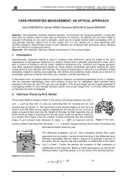
Surface spectral moments• Surface spectral moments mp,qmareωpωqp, q=1 2S1,2) d1d∫∫( ω ω ω ωS( ω 1, ω2)is bivariate power spectral density of surface.Necessary condition for the case of degenerated spectrum(one dimensional) is2( m m − m ) =2 ,0 0,2 1,1For degeneration to the more dimensions the similarconditions can be derived202

Profile and surface spectralmomentsm r• The profile spectral moment in thedirection θ is connected with surfacemoments mp,q by relationmr(θ )r ⎛n⎞r−1( θ)= mr, 0cos θ + ⎜ ⎟mr−1,1cos θ sinθ+ .. + m0,⎝1⎠m 2( θThe second profile spectral moment )is equal to the variance of profile slope PS 2rsin2m2( θ ) = m2,0*cos θ + 2* m1,1*cosθ*sinθ+ m0,2* sinIt is then possible to estimate the surface moments m 2,0,m 1,1and m 0,2by using of linear regression.rθ2θ

AnisotropycharacteristicsLong-crestedness 1/gg =2min2max• For an isotropic surface is g = 1 and for degeneratedone dimensional spectrum is g = 0.Anisotropy AN2* m2 ,0* m0,2− mAN = 1−• For AN = 0 is surface perfectly isotropic and form2,0AN+=m10,2issurface anisotropic. Lower AN characteristic indicates lowdegree of anisotropy.mm21,1

MaterialThe three types of weaves have been selected:Sample I A- Krull (surface loops)Sample II B - TwillSample III C – Plain (low sett)

Measurement• For investigation of influenceof surface roughness directionon fractal dimension and classical roughnesscharacteristics the three fabrics with differentweaves were selected.• The R(x) traces have been obtained by means ofKES apparatus in the following directions: 0deg(weft direction), 30deg, 45deg, 60deg and 90deg(warp direction).• The standard conditions of measurements wereused.

ResultsWeave m 2,0m 1,1m 0,2ANA 0.767066 0.06126 0.15058 0.2714B 0.0020481 -0.0250 0.2293 1C 1.0306 -0.8780 0.73729 1

Sample Afractal dimension mean = 1.90895.fractal dimension init= 1.68005.

Sample Bfractal dimension mean = 1.96176.fractal dimension init = 1.85573.

Sample Cfractal dimension mean = 1.97429.fractal dimension init = 1.94088.

Anisotropy – plain weave

Anisotropy – twill

Conclusion•The proposed technique iscapable to estimate roughnesscharacteristics of anisotropicsurfaces typical for textile structures•Beside the anisotropy measure AN the principaldirection and values of m2max will be probablynecessary for deeper description of textilessurface roughness

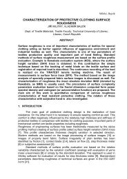
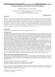
ANISOTROPY OF SURFACE ROUGHNESSJiří Militký , Martin Bleša and J VidourkováTechnical University of LiberecHalkova street No 6, 461 17 Liberec, Czech Republice - mail : jiri.militky@vslib.czABSTRACTClassical method of surface roughness measurements is based or the surface profilemeasurement. Characteristic of roughness is then variation coefficient of surface profile[surface height variation]. This approach is correct for so called isotropic random surfaces.Majority of textile structures have anisotropic surface and therefore it is necessary tocharacterize the degree of anisotropy as well. Rough data sets are so called surface heightvariations (SHV) traces in selected angles according to cross direction. From these data setsthe surface spectral moments are computed. The principal direction of roughness and somemeasures of anisotropy are proposed. The estimation of SHV traces complexity in individualdirections is based on the spectral power density and variogram [structure function]. Theconcept of fractal dimension is proposed. The applicability of proposed approach isdemonstrated on the three fabrics with different surface appearance.KEYWORDS: Surface roughness, variogram, roughness anisotropy, and spectral moments1. INTRODUCTIONRoughness of textiles is important parameter influencing subjective hand feeling andconnected with behavior of textiles layers in mutual contact (due to interlayer friction).Traditional stylus profiling method produces data as one dimensional height variation in theselected direction of rough surface. This roughness profile is called surface height variation(SHV) trace [1]. For SHV characterization the standard roughness parameters described in theISO 4287 are frequently used [2]. This approach is used in Shirley software for evaluation ofresults for step thickness meter [3]. Kawabata [4] constructed measuring device forregistration the surface height variation (SHV) trace. The main part of this device is contactorin the form of wire (diameter 0.5 mm). This contactor is moved by constant rate 0.1 cm/secand SHV is registered on paper sheet. The sample length L=3 cm is used. The SHVcorresponds to the surface profile in selected direction (usually in the weft and warpdirections are used for SHV creation). The result of measurements is thickness R(d) in variousdistances d from origin. Characterization of roughness based on the mean absolute deviationMAD is the classical descriptive statistical approach [5]. There exists a vast number ofempirical profile or surface roughness characteristics suitable often in very special situations[6].Above-mentioned roughness characteristics have implicitly assumed that surfaceroughness is isotropic phenomenon. This assumption can be accepted in the cases whensurfaces have the same micro geometric properties no matter what direction they areinvestigated in. Majority of textiles structures have anisotropic nature. Surface of wovenfabric is clearly patterned due to nearly regular arrangements of weft and warp yarns. Thespecial non-random patterns are visible on knittings as well. It is well known that anisotropyof mechanical and geometrical properties of textile fabrics are caused by the pattern and nonisotropicarrangement of fibrous mass. Periodic fluctuations of surface heights can bespatially dependent due to arrangements of yarns. Non-periodic complexity spatialdependence is subtler. The roughness characteristics computed from SHV trace are thereforedependent on the direction of measurements i.e. angle of transect line according to fabric

cross direction (perpendicular to machine direction). In KES system is possible anisotropytreated by averaging of roughness parameters in weft and warp directions only. This approachis generally over simplified and can leads to under or over estimation of surface roughness.For characterization of anisotropy here is proposed to measure a set of surface profilesin selected directions (angles). For description of roughness angular dependence the so-calledprofile spectral moments are used because there exists a relation between these 2D momentsand 3D surface moments [7]. The principal direction of roughness and some measures ofanisotropy can be now computed from estimated 3D surface moments [8]. This approach toroughness anisotropy evaluation is here demonstrated on the three fabrics with differentsurface appearance.2. SHV PROFILE ROUGHNESS CHARACTERISTICSStarting point for characterization of surface roughness are characteristics of surfaceprofiles in selected angles θ according to the cross direction axis. In this section the typicalcharacteristics of profile roughness are described. Because of the computation procedure forcharacteristics is the same for all directions the symbol for angle is omitted here. From theSHV trace is possible to evaluate a lot of roughness parameters. All roughness parameters arebased on the set of points R(x j ) j =1.. M defined on the sample length interval L. Themeasurement points x j are obviously selected as equidistant and then R(x j ) can be replaced bythe variable R j . For identification of positions in length scale is sufficient to know samplingdistance x s = x j - x j-1 = L/M for j>1. A set of parameters for profile characterization iscollected in [8]. These parameters are divided to the following groups:• Statistical characteristics of height geometry or height distribution (variance, skewness,kurtosis)• Spatial characteristics as autocorrelation or variogram (denoted in engineering asstructural function)• Spectral characteristics based on the power spectral density PSD• Functional characteristics (connected with fluid retention or flow properties)Spatial and spectral characteristics are closely connected with characteristics computed fromfractal models (fractal dimension and topothesy). There exist some interconnections betweenclassical geometrical characteristics and spectral moments computed from PSD as well.2.1 STANDARD ROUGHNESS CHARACTERISTICSThe standard roughness parameters used frequently in practice are [22]:(i) Mean Absolute Deviation MAD. This parameter is equal to the mean absolute difference ofsurface heights from average value (R a ). For a surface profile this is given by∑MAD =1 R j− R a(1)M jThis parameter is often useful for quality control. However, it does not distinguish betweenprofiles of different shapes. Its properties are known for the case when R j ’s are independentidentically distributed (.i.i.d.) random variables(ii) Standard Deviation (Root Mean Square) Value SD. This is given by12SD = ∑(R j− R a)MjIts properties are known for the case when R j ’s are independent identically distributed (.i.i.d.)random variables. One advantage of SD over MAD is that for normally distributed data can(2)

e simple to derive confidence interval and to realize statistical tests. SD is always higher thanMAD and for normal data is SD = 1.25 MAD. It does not distinguish between profiles ofdifferent shapes as well. The parameter SD is less suitable than MAD for monitoring certainsurfaces having large deviations (corresponding distribution has heavy tail).(iii) Mean Height of Peaks MP. This is calculated as the average of the profile deviationsabove the reference value R (often is R = R a ). It is given as mean value of peaks P i , i = NpwherePi= Ri− R for R i− R > 0 and Pi= 0 elsewhere(iv) Mean Height of Valleys MV. This is calculated as the average of the profile deviationsbelow the reference value R (often is R = R a .). It is given as mean value of valleys V i , i = NvwhereVi = R − R ifor R i− R < 0 and Vi= 0 elsewhereThe parameters MP and MV give information on the profile complexity. Exceptional peaks orvalleys are not considered but are useful in tribological applications.(v) The Standard Deviation of Profile Slope PS. This is given by21 ⎛ dR(x)⎞PS = ∑⎜⎟ (3)M j ⎝ dx ⎠j(vi) The Standard Deviation of Profile Curvature PC. This quantity called often as waviness isdefined by the similar way22PC 1∑ ⎛ d R(x)2M j dx⎟ ⎞⎜⎝ ⎠ j= (4)The slope and curvature are characteristics of a profile shape. The PS parameter is useful intribological applications. The lower the slope the smaller will be the friction and wear. Also,the reflectance property of a surface increases in the case of small PS or PD.(vii) Mean Slope of the Profile MS. This is given byMS=1M∑jdR(x)dxj(5)Mean slope is an important parameter in several applications such as in the estimation ofsliding friction and in the study of the reflectance of light from surfaces.(viii) Ten Point Average TP. This characteristic is defined as the average difference betweenthe five highest peaks and five deepest valleys within a surface profile. The parameter TP issensitive to the presence of high peaks or deep scratches in the surface and is preferred forquality control purposes.These parameters are useful in the case of functional surfaces or for characterizing surfacebearing and fluid retention and other relevant properties. For the characterization of hand willbe probably best to use waviness PC. The characteristics of slope and curvature can becomputed for the case of fractal surfaces from power spectral density, autocorrelation functionor variogram. For computation of above-mentioned characteristics the program DRSNOST inMATLAB has been created.

2.2 ROUGHNESS IN SPECTRAL DOMAINSpectral analysis provides an essential tool for the understanding the frequencycomponents of a profile roughness. The primary tool for evaluation of periodicities isexpressing of signal R(x) by the Fourier series of sine and cosine waves. The Fouriertransform is conversion of data from series according to x to the series offrequencies ω = 2π* k /( M * L), for k=1, 2, 3…∑RF( ω ) = R(x) * exp( −i* ω * x)(6)Function RF is symmetric about frequencyω = π / L . For discrete data the fast FourierTransform (FFT) leads to transformed complex vector DRF. Vector DRF may be used forcreation of power spectral density. PSD = S(ω)PSD =22 2= S( ω ) = DRF * conj(DRF)/ L abs(DRF)/ L(7)where conj(.) denotes conjugate vector. The S(ω) is estimator of spectral density function andcontains values corresponding to contribution of each frequency to the total variance of R(d).Frequency of global maxim on S(ω) is corresponding to the length of repeated pattern andheight corresponds to the no uniformity of this pattern. Spectral density function is thereforegenerally useful for evaluation of hidden periodicities.The estimation of the spectral density function S(ω) is relatively straightforward intheory but in practice situation is more difficult since data are only available in discretesamples of limited extent. For finite sample lengths if is necessary to use windowing(avoiding leakage) de-trending (avoiding non stationarity of mean) and filtration of parasitefrequencies.The rough profiles are often random, multiscaled and disordered. The main property oftheses profiles is self-affinity due to similarity in appearance under different magnifications.The typical is Weistrass Mandelbrot equation, which satisfies to the self-affinity requirement(replaces of self similarity for case of functions). The height R (x) of profile in the point x ofSHV trace is equal to∑ ∞ iD−1 cos(2π* g x)R(x)= G(8)i*(2−D)i=n g1where 1

2.3 ROUGHNESS IN SPATIAL DOMAINIt is well known that the spectral analysis is suitable for the stationary random seriesonly (“detrend” operation should be therefore used). The same information can be obtainedfrom the statistical characteristics. These characteristics are generally more stable and simplerto computation. A basic statistical feature of R(x) in the spatial domain is autocorrelationbetween distances. Autocorrelation depends on the lag h (i.e. selected distances betweenplaces of measurement). The main characteristics of autocorrelation is covariance functionC(h)C ( h)= cov( R(x),R(x + h))(11)and autocorrelation function ACF(h) defined as normalized version of C(h)C(h)ACF ( h)= (12)C(0)ACF is one of main characteristics for detection of short and long-range dependencies indynamic series. It could be used for preliminary inspection of data. The computation ofsample autocorrelation directly from definition is for large data tedious. The ACF is inverseFourier transform of spectral density∞∫0ACF ( h)= S(ω)exp( i ω h)dω(13)This relation shows that characteristics in the space and frequency domain areinterchangeable.In spatial statistics is more frequent variogram, (called often as structure function)which is defined as one half variance of differences (R(x) - R(x+h))Γ ( h ) = 0.5 D[R(x)− R(x + h)](14)The variogram is relatively simpler to calculate and assumes a weaker model of statisticalstationarity, than the power spectrum. Several estimators have been suggested for thevariogram. The traditional estimator isM ( h)1G ( h)( R(x j ) − R(x j+h2M( h)j=12= ∑ )(15)where M(h) is the number of pairs of observations separated by lag h. It can be summarizedthat simple statistical characteristics are able to identify the periodicities in data but thereconstruction of “clean” dependence is more complicated. The variogram is often sufficientfor characterization of surface profiles. The fractal dimension can be computed from powerlaw dependence of variogram similar to the power dependence of power spectral density (seeeqn. (16)).2.4 FRACTAL DIMENSIONThe term of fractal dimension is not perfectly unique. There are several definitions offractal dimension D. For the same roughness profile the numerical values of fractal dimensioncomputed from various definitions are usually only slightly different. Most procedures offractal dimension determination are based on the power law. These laws are generallyg ( D)expressed by the relation f ( x)= a*x , where the exponent g(D) depends on the fractal

dimension only. The measuring of x and f(x) depends on the law used. For the Box countingmethod is x equal to line distant of square grid and f(x) is area of all grid boxes striking theobject (roughness profile). The g(D)=-D. For a power law variogram is validHΓ ( h ) ≈ c h(16)where c is a constant. The Hurst exponent H, lies in the interval (0,1). Where H = 0 thisdenotes a curve of extreme irregularity and H = 1 denotes a smooth curve. Exponents H andfractal dimension D are in fact related D = 2-H. Fractal dimension is conventionally obtainedthrough estimating the parameter from a LSE linear regression of the log-log transformationof Equations (9) and (16). In practice is behavior expressed by eqn. (16) valid near origin andby enq (9) in a neighborhood of infinity. In general, it s D computed from this relationdenoted as effective fractal dimension.Based on these equations the program DRSNOST in MATLAB for estimation offractal dimension from variogram has been constructed. From the first 10 points the initialfractal dimension D Fp and from all points the mean fractal dimension D F are computed.3. SURFACE ROUGHNESS DESCRIPTIONThere are two main reasons for measuring surface roughness. First, is to controlmanufacture and second is to help to ensure that the products perform well. In the textilebranch the former is the case of special finishing (e.g. pressing or ironing) but the later isconnected with comfort appearance and hand.From a general point of view, the rough surface display process which have two basicgeometrical features:(1) Random aspect: the rough surface can vary considerably in space in a random manner,and subsequently there is no spatial function being able to describe the geometricalform,(2) Structural aspect: the variances of roughness are not completely independent withrespect to their spatial positions, but their correlation depends on the distance.Especially surface of weaves is characterized by nearly repeating patterns andtherefore some periodicities are often identified.The fractal dimension of isotropic surfaces is simply 1+ fractal dimension of any profile. Thesituation for anisotropic surfaces is more complicated. For weakly anisotropic surfaces(stretched in the one dimension only) the fractal dimension is independent on the angle ofmeasurementθ . For the strongly anisotropic surfaces are fractal s dimension changed (thefractal dimension along the direction of lines in pattern is less) [9]. Longuet-Higgins [10]proposed for anisotropic surfaces to use so called surface spectral moments m p,q defined byrelationp qm = ω ω S( ω , ω ) dωω(17)∫∫p, q1 2 1 2 1d2where S ω 1, ω ) is bivariate power spectral density of surface. Necessary condition for the(22case of degenerated spectrum (one dimensional) is 2( m2 ,0m0,2− m1,1) = 0 . For degeneration tothe more dimensions the similar conditions can be derived [10]. The profile spectral momentmr(θ ) in the direction θ defined by eqn. (10) is connected with surface moments m p,q byrelationr ⎛n⎞r−1rmr( θ ) = mr, 0cos θ + ⎜ ⎟mr− 1,1cos θ sinθ+ .. + m0,rsin θ(18)⎝1⎠

The second profile spectral moment m2(θ ) , which is equal to the variance of profile slopePS 2 , is function of three surface moments m 2,0 , m 1,1 and m 0,2 only. This dependence has thesimple form derived directly from eqn. (18)2m2( θ ) = m2,0*cos θ + 2* m1,1*cosθ*sinθ+ m0,2* sin2θ(19)The surface moments play central role in description of surfaces topography. The parametersm 2,0 and m 0,2 , which are the 2 nd surface spectral moments, denote the variance of slope in twovertical directions along cross direction and machine direction. The parameter m 1,1 representsthe association-variance of slope in these two directions. These parameters are generallydependent of the selected coordinate system. From the known values of m ( θ ) for selectedset of directions θii = 1,..n it is possible to estimate the surface moments m 2,0 , m 1,1 and m 0,2by using of linear regression. The maxima and minima of eqn. (19) are2 2( m , m ) = 0,5*[( m + m ) ± {( m − m ) + 4 }](20)2 max 2 min2,0 0,22,0 0,2m1,1These occurs in the angle θpcalled principal direction given by relationtan2m1,1θp=(21)m2,0− m0,2As one measure of anisotropy the so-called long-crestedness 1/g has been proposed in [10]wherem2 ming = (22)m2 maxFor an isotropic surface is g = 1 and for degenerated one-dimensional spectrum is g = 0.The better criterion of anisotropy has been proposed in [5]2,00,221,12* m2 ,0* m0,2− mAN = 1−(23)m + mFor AN = 0 is surface perfectly isotropic and for AN = 1 is surface anisotropic. LowerAN characteristic indicates low degree of anisotropy.4. EXPERIMENTSFor investigation of influence of surface roughness direction on fractal dimension andclassical roughness characteristics the three fabrics with different weaves were selected. TheR(x) traces have been obtained by means of KES apparatus in the following directions: =í2 iθ 0 o(weft direction), 30 o , 45 o , 60 o and 90 o (warp direction). The standard conditions ofmeasurements were used.5. RESULTS AND DISCUSSIONThe geometrical characteristics and fractal dimensions of individual profiles at chosendirections θíwere computed and plotted as polar graphs. These graphs are summarized in[11]. The surface moments m 2,0 , m 0,2 and m 1,1 were computed from eqn. (19) by using of linearleast squares regression. Estimated surface moments and AN anisotropy measure are given inthe table I. The angular dependence of profile slope variance form eqn.(19) and experimentalpoints are shown on the figure 1.

Table I. Surface moments and anisotropy of samplesPattern Weave m 2,0 m 1,1 m 0,2 AN-anisotropyA- Krull surfaceloops0.767066 0.06126 0.150587 0.2714B - Twill 0.0020481 -0.0250585 0.229335 1C – PlainLow sett1.0306 -0.878057 0.73729 1.A B CFig. 1. Profile slope variance angular dependence (crosses) and predicted slope variance(solid line) for samples from table I.The results of computation are in good agreement with visual roughness appearance.6. CONCLUSIONThe proposed technique is capable to estimate roughness characteristics of anisotropicsurfaces typical for textile structures. Beside the anisotropy measure AN the direction θpandvalues of m 2max will be probably necessary for deeper description of textiles surface roughnessThis work was supported by the research project of Czech Ministry of Education LN00B09010. REFERENCES[1] Militký J, Bajzík.V: Description of thickness variation by fractal dimension, Proc. Conf.STRUTEX 2000, Liberec December (in Czech) (2000)[2] ISO 4287: Geometrical product specification, GPS-surface texture, profile method - terms,definitions, and surface texture parameters, Beuth Verlag, Berlin 1997[3] Anonym: Operation Manual, Shirley(1999)[4] Kawabata S.:Text. Mach. Soc. Japan (1980)[5] Meloun M., Militky J., Forina M.: Chemometrics for Analytic Chemistry vol. I, StatisticalData Analysis, Ellis Horwood, Chichester (1992)[6] Militký J., Bajzík V.: Characterization of textiles surface roughness, Proc. 7 th Int. AsianTextile Conference, Hong Kong August 2001[7] Li Ch. G. et. all: Wear 237,211, (2000)[8] Nayak P. R.: Trans. ASME : J. Lub. Tech. 93F, 398 (1971)[9] Thomas T. R., Roson B. G., Amini N.: Wear 232, 41 (1999)[10] Longuet-Higgins M.S.: Phil. Trans. R. Soc. London, A 250, 157, (1957)[11] Militký J.: work to be published (conference in Dubrovnik), (October 2004)