Speech Recognition by Using LPC Parameters

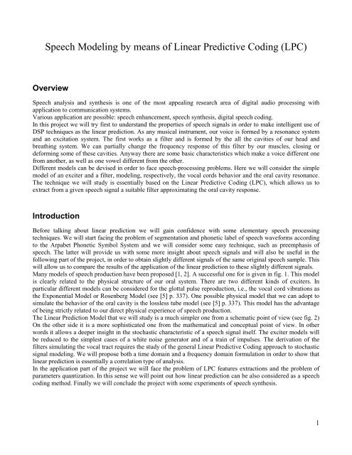
Speech Modeling by means of Linear Predictive Coding (LPC)OverviewSpeech analysis and synthesis is one of the most appealing research area of digital audio processing withapplication to communication systems.Various application are possible: speech enhancement, speech synthesis, digital speech coding.In this project we will try first to understand the properties of speech signals in order to make intelligent use ofDSP techniques as the linear prediction. As any musical instrument, our voice is formed by a resonance systemand an excitation system. The first works as a filter and is formed by the all the cavities of our head andbreathing system. We can partially change the frequency response of this filter by our muscles, closing ordeforming some of these cavities. Anyway there are some basic characteristics which make a voice different onefrom another, as well as one vowel different from the other.Different models can be devised in order to face speech-processing problems. Here we will consider the simplemodel of an exciter and a filter, modeling, respectively, the vocal cords behavior and the oral cavity resonance.The technique we will study is essentially based on the Linear Predictive Coding (LPC), which allows us toextract from a given speech signal a suitable filter approximating the oral cavity response.IntroductionBefore talking about linear prediction we will gain confidence with some elementary speech processingtechniques. We will start facing the problem of segmentation and phonetic label of speech waveforms accordingto the Arpabet Phonetic Symbol System and we will consider some easy technique, such as preemphasis ofspeech. The latter will provide us with some more insight about speech signals and will also be useful in thefollowing part of the project, in order to obtain slightly different signals of the same original speech sample. Thiswill allow us to compare the results of the application of the linear prediction to these slightly different signals.Many models of speech production have been proposed [1, 2]. A successful one for is given in fig. 1. This modelis clearly related to the physical structure of our oral system. There are two different kinds of exciters. Inparticular different models can be considered for the glottal pulse reproduction, i.e., the vocal cord vibrations asthe Exponential Model or Rosenberg Model (see [5] p. 337). One possible physical model that we can adopt tosimulate the behavior of the oral cavity is the lossless tube model (see [5] p. 337). This model has the advantageof being strictly related to our direct physical experience of speech production.The Linear Prediction Model that we will study is a much simpler one from a schematic point of view (see fig. 2)On the other side it is a more sophisticated one from the mathematical and conceptual point of view. In otherwords it allows a deeper insight in the stochastic characteristic of a speech signal itself. The exciter models willbe reduced to the simplest cases of a white noise generator and of a train of impulses. The derivation of thefilters simulating the vocal tract requires the study of the general Linear Predictive Coding approach to stochasticsignal modeling. We will propose both a time domain and a frequency domain formulation in order to show thatlinear prediction is essentially a correlation type of analysis.In the application part of the project we will face the problem of LPC features extractions and the problem ofparameters quantization. In this sense we will point out how linear prediction can be also considered as a speechcoding method. Finally we will conclude the project with some experiments of speech synthesis.1

Fig. 1: A physical model for speech production1. A preliminary approach to speech processingSegmentation and phonetic label of speech waveforms is a fundamental problem in speech processing.Automatic segmentation is not an easy task to carry out. As a preliminary step is very instructive to perform amanual segmentation of a given speech waveform and to identify the different phonemes of the utterance.Question 1: Load the file phrase.wav (sr=11025) in matlab using the function wavread and listen to it by meansof the function sound. Write down a phonetic representation of the speech waveform using the ARPABETPhonetic Symbol System (see Table 1). Then plot the signal vector phrase. Print the figure and write out whereeach phoneme begins and ends. (Use the function plot and subplot)Table 1 ARPABET Phonetic Symbol System2

Question 2: From phrase create two signals, the first one containing the vowels of the sentence (utterance 1)and the second the consonants (utterance 2) (Hint: substitute matrices of zeros by the function zeros to obtainUtterance 1. When you have the original utterance how can you immediately compute utterance 2?)Now we could ask ourselves what are the main differences and the similarities between utterance 1 and utterance2. The voice has the same "timbre" in both signals, in the sense that we are able to say that is the same personspeaking. On the other hand everybody knows from his own experience how the pronunciation of a vowel isdifferent from that of a consonant. Voiced sounds are produced by a sustained emission of breath plus a"vibration of the vocal cords". The fricative consonants (f, th, s, sh) are produced by a sustained emission ofbreath but without a "vibration of the vocal cords". The plosive consonants (k, p, t) are produced by closing andrapidly opening the vocal cavity. In every case the differences between one sound and the other is determined bythe position of the oral cavity, the lips and the tongue. In other words the air passes from the lungs into the vocaltract, which is a series of cavities acting as resonators, emphasizing some frequencies and attenuating others.These resonances are called formants. The formants are the main "timbrical print", which allows us todistinguish between a male, a female and a child voice as well as between different voices of the same sex andage.The following study of the Linear Prediction Technique aim is to model the formants, i.e., to find the filterproviding a good approximation of the effect of the vocal tract on the excitation.We have also to define a model for the excitation, i.e. the breath and the “vibration of the vocal cords”, the socalled glottal impulses. In the LPC representation the excitation models are the simplest that one can devise. Thebreath sound can be approximated by some more or less colored noisy signal. The glottal impulses are on theother side equivalent to simple impulse trains of the kind:whereNn=0( i − nP)f ( i)= δ (1)1n = 0δ ( n)= (2)0n ≠ 0Question 3: Produce a single impulse signal δ(0) and a white noise signal (use the function rand). What aretheir spectra. Comment the result. Then take a train of impulses. What is its spectrum? How does the spectrumchange if you increase or decrease the number of impulses? Comment the result.In general we can think about consonants as unvoiced, noisy sounds producing turbulence in the vocal tract.Voiced sounds are characterized by trains of impulses exciting the resonances of the vocal tract.How can we "separate" the vocal tract form the excitation in a given speech signal? In order to find the answer tothis question we have to study the linear prediction theory.Before facing this problem, in order to gain some more confidence with speech signals processing we considerone of the simplest speech processing application: Preemphasis of Speech.Speech signals have a spectrum that falls off at high frequency. Preemphasis is a technique, which compensatethis fall off. This compensation is obtained by means of a “first difference” filter of the kind:y[n]=x[n]-αx[n-1] (3)3

where x[n] is the input signal, y[n] is the preemphasized signal and α a parameter.Question 4: What is the impulse response of the filter. Use freqz to plot the frequency response of the system forα = .5, .9, .98. Apply the filter to the signal phrase. Which α provide a better emphasis? Use alternatively filterand conv to implement the preemphasis filters. What are the differences between the two functions (see the helponline) and between the two outputs?2. Linear Prediction2.1. Basic TheoryThe main idea of linear prediction is to model a signal as a linear combination of: a) its past values and b)present and past values of a hypothetical input to a system whose output is the given signal. The previousstatement mathematically translated gives:sK[ n] = −as[ n − k] + Gblu[ n − l] , b0= 1k = 1Lk, (4)l = 0where the a k , the b k and the gain G are the parameters of the hypothetical system and the s[n-k] are the pastvalues of the signal and the u[n-k] are the samples of the hypothetical input.In the frequency domain, by taking the z-transform on both sides of (4), we obtain:L−l1 + blzS(z)l=1H ( z)= = G(5)KU(z)−k1 + a zQuestion 5: Derive equation (5) from equation (4) (Hint: exchange the sum order between the index n and thetwo indexes l and k).In other words equation (4) tell us that a signal s[n] is predictable from its past and some inputs to a certainsystem H(z).There are two special cases of interests:1) a k =0, for 1

GH ( z)=(7)1+Kk=1We assume that the input u[n] is totally unknown and the signal s[n] can be predicted only approximately from alinearly weighted summation of past samples. Let this approximation of s[n] be ~ s [ n ] , where:Then we can define the error or the residual as:Ka k z−k[] n = −aks[ n − k]~ s(8)k=1[] n − ~ s [] n = s[] n + aks[ n − k]Ke[ n]= s(9)k=1Fig. 2: LPC model as a time-varying linear systemAt this point we have to use some error minimization method in order to compute the parameters a k . We candecide to use the method of the least squares. The a k are then obtained as a result of the minimization of themean of total squared error with respect to each of the parameters a k .Our speech signal is actually a stochastic signal and its voiced segments are wide sense stationary stochasticprocesses. The error e n is a sample of a random process, therefore in the least squares method we minimize theexpected value of the square of the error:Now we have to differentiate with respect to each parameter:K22 Err = E( e[n]) = Es[ n] + aks[ n − k] (10) k = 1 ∂(Err)∂ak= 0 ,for 1 ≤ k≤ K(11)We obtain:− EK( s[][ n s n − i]) = akE( s[ n − k] s[ n − i])k=1(12)5

The minimum average error is given by:ErrKK2( s[]n ) + a E( s[][ n s n − k])= E k=1k(13)Question 6: Derive equation (13) from equations (10) and (12).For a stationary process s[n] we know that:E( s[ n k] s[ n − i]) = R( i − k)− (14),where R(i) is the autocorrelation of the process. Equations (12) and (13) reduce then to:− Rknown as Yule-Walker equations andK() i = a R( i − k ),1 ≤ i ≤ Kk=1k, (15)ErrkK() + a R()k= R 0 , (16)k=1krespectively.In the non-stationary case we have:E( s[ n k] s[ n − i]) = R( n − i,n − k)− (17)Without loss of generality (why?), we can consider the autocorrelation at time n=0 and the (17) becomes− RK( 0, −i) = a R( − k,−i) , 1 ≤ i ≤ Kk=1k(18)K( 0,0) + a R( 0 k )Errk = Rk,(19)It is important to note that for a certain class of non-stationary processes known as locally stationary processes, itis reasonable to estimate the autocorrelation function with respect to a point in time as a short-time average(local ergodicity). Speech is one example of non-stationary process, which can be considered to be locallystationary.Question 7: Show that for stationary signal the normal equations (18) and (19) reduce to the (15) and (16)respectively.k=16

2.2. Input modelsWe now consider two particular types of input that are of special interest: the deterministic impulse and thestationary white noisea) Impulse input: Let the input to the all-pole filter H(z) be an impulse or unite sample at n=0, i.e., u[n]=δ[n].The output of the filter H(z) is then its impulse response h[n]:hK[] n − a h[ n − k] + Gδ[ n]= k=1k(20)The autocorrelation R h (i) of the impulse response h[n] has a very interesting relationship to the autocorrelationR s (i) of s[n]. Multiplying (20) by h[n-i] and summing over all n we obtain:and− RK() i = a R ( i − k) , ≤ i ≤ ∞h k h1k=1, (21)RK2() 0 − a R () k G= h k h+k=1for i=0 (22)Question 8: Derive equations (21) and (22). Note that the filter h is causal.If we impose the condition that the total energy in h[n] must equal that in s[n], we must have:R() 0 R () 0 R()0= (23)h s=hRs?From the (23) and the similarity between (21) and (15) we can conclude that:Question 9: What is the meaning of R ( 0)and ( 0)R() i R () i R()i= 0

) White noise input: The input are mutually uncorrelated, zero-mean samples, i.e., E(u[n])=0 and unit varianceE(u[n]u[m])=δ n,m . Denote the output of the filter by s w [n]:sK[] n − a s [ n − k] Gu[n]= w k w+k=1(26)Question 10: Is s w [n] stationary or not?Multiplying the (26) by s w[ n − i]and taking the expected values and noting that the u[n] and the s w[] n areuncorrelated for i>0, we obtain the usual Yule-Walker equations. Similarly to the previous case we require thatthe average energy (or variance) of the output s w[] n be equal to the energy of the original signal s [] n , orR w (0)=R s (0), since the zero th autocorrelation of a zero-mean random process is the variance. By reasoning similarto that given in the previous section, we conclude that (24) and (25) apply also for the random case.From the previous discussion we see how the relations linking the autocorrelation coefficients of the output of anall-pole filter are the same whether the input is a single impulse or white noise. This is to be expected since bothtypes of input have identical autocorrelation and, of course, identical flat spectra.This dualism between the deterministic impulse and statistical white noise is once more very appealing.The predictor coefficients a k , 1

2.3. Frequency Domain FormulationNow we see how the same results can be derived from a frequency domain formulation. It will become clearthat linear prediction is basically a correlation type of analysis, which can be approached either from thetime or from the frequency domain.Applying the z transform to (9) representing the error e[n] between the actual signal and the predicted signal, weobtain:where A(z) is the inverse filter:E(z)K k 1+ ak z S(z)= A(z)S(z)(28) k = 1 =−and E(z) and S(z) are the z transform of e[n] and s[n] respectively.Applying the Parseval Theorem, the total error to be minimized is given by:AK−k( z)= 1 + a kz(29)k=1Err =∞2 enn=−∞=12ππ−πEj( e )ω 2dω(30)jωwhere E ( e ) is obtained by evaluating E(z) on the unit circlesignal s[n] by P(ω), where:z = ejω. Denoting the power spectrum of thejω( e ) 2P ( ω)= S(31)we have from (28)-(31)1 πErr = P ω A eπ ( )2 − πjω− jω( ) A( e ) dω(32)Following the same procedure as in the previous section Err is minimized by applying (11) to (32). The resultcan be shown to be identical to the Yule-Walker equation [8], but with the autocorrelation R(i) obtained from thesignal spectrum P(ω) by an inverse Fourier transform.1 πjiωR( i)= P ω e dωπ ( )(33)2 − π9

2.4. Linear Predictive Spectral MatchingIn this section we shall examine in what manner the signal spectrum P(ω) is approximated by the all-pole modelspectrum, which we shall denote by P H (ω). From (7) and (29):PFrom (28) and (31) we have:22jω2 GGω ) = H ( e ) = =(34)jω2KA(e )− jkω1 + a eH(2k=1k2jωE(e )P ( ω)= (35)jω2A(e )By comparing (34) and (35) we see that if P(ω) is being modeled by P H (ω). Then the error power spectrum2jωE ( e ) is being modeled by a flat spectrum equal to G 2 . This means that the actual error signal e[n] is beingapproximated by another signal that has a flat spectrum, such as a unit impulse, white noise or any other signalwith a flat spectrum. The filter A(z) is called the "whitening filter" since it attempts to produce an output signalthat is white, i.e., has a flat spectrum.From (30), (34) and (35), the total error can be written as:2GErr =2ππ − πP(ω)dωP ( ω)H(36)We can restate the problem of linear prediction as follows. Given some spectrum P(ω) we wish to model itby another spectrum P H (ω) such that the integrated ratio between the two spectra in (36) is minimized.The parameters of the model spectrum are computed from the normal equation (15), where the neededautocorrelation coefficients R(i) are easily computed from P(ω) by a simple Fourier Transform. The gain factorG is obtained by equating the total energy in two spectra, i.e., R H (0)=R(0), where as usual:RH1 πjiω( i)= PHω e dωπ ( )(37)2 − πFrom (24) we have R( i)= RH( i), 0

the spectrum is computed, it is quite important to properly choose the type and width of the data window to beused. The choice depends very much on the type of signal to be analyzed. If the signal can be considered to bestationary for a long period of time then a rectangular window suffices. However in many transient speechsounds, the signal can be considered stationary for a duration of only one or two pitch periods. In that case awindow such as Hamming or Hanning is more appropriate.3. Applications3.1. Predictor Filter ComputationCompute the predictor parameters of a 12 th –order filter for two phonemes, an AA and a SH extracted from theword "tache" in the phrase signal. Use a Hamming window of length 512 samples. For both phonemes make adB plot of the frequency response of the prediction error filter and of the vocal tract model (use the Matlabfunction lpc and have a look to the help). Also use roots and zplane to plot the zeros of the prediction error filterfor both cases.Question 12:a) What do you observe about the relationship between the zeros of the prediction error filter and: 1) the poles ofthe vocal tract model filter; 2) the peaks in the frequency response of the vocal tract model filter.b) Compute the Fourier transform of the windowed segments of speech, and its magnitude in dB and compare itwith the vocal tract model. Comment the result.c) Try to vary the model order and apply the technique to other speech segments and observe the effectsd) Repeat the experiments of the first two phonemes with a preemphasized version of the signal (with α=0.98).Compare the results with and without preemphasis.e) Finally, use the prediction error filters to compute the prediction error sequence e[n] for both phonemes. Usesubplot to make a two panel subplot of the (unwindowed) speech segment on the top and the prediction error onthe bottom part of the plot. What do you observe about the differences in the two phonemes? Where do the peaksof the prediction error occurs in the two cases?3.2. Formant TrackingThe roots of A(z) (i.e., the poles of the vocal tract filter) are representative of the formant peak frequencies. Inother words, the angles of the roots, expressed in terms of analog frequencies can be used as an estimate of theformant frequencies. We want now to plot the formant frequencies as a function of the frame number, i.e., oftime, in order to observe the time-evolution of the vocal tract filter.Question 13:a) Compute the LPC coefficients for a Hamming windowed speech segment.b) Find the frequencies corresponding to the angles of the zeros of the predictor filter.c) Repeat the operation 100 times at lags of half the window length.d) Plot the matrix of the results using any discrete symbol (see plot help), in order to obtain a figure similar tofig. 3.11

Fig. 3 Formant trackingYou can note from fig. 3 that the previous algorithm plots all the frequencies, including those corresponding toreal roots (ω=0 and ω =π). Also, it might plot the frequencies corresponding to complex roots twice. It isdesirable to eliminate these values, which are obviously not formant frequencies. It is also quite likely that rootswhose magnitude is less than 0.8 are not formants.Question 14: Use the find function to locate the roots to be eliminated. Replace them in the formant matrix bythe object NaN,(not a number) in order to preserve vectors lengths. The function plot will automatically ignorethe NaN values.3.3. Phonemes SynthesisAs a final step of this project we try to reproduce synthetically the two analyzed phonemes. We know that inorder to simulate a vowel we need an impulse train exciter, whereas we need a noise generator in order tosimulate a fricative consonant.Question 15:a) Use an impulse train as an input to the previously extracted vocal tract filter. Find a pitch for an impulsetrain providing a good approximation of the phoneme AA.b) Use a random generator (rand) as an input to the second vocal tract filter model, in order to reproduce thephoneme SH.c) Adopting a Hamming window try to maintain the original transient of the phonemes and use the synthesizedsignals for the following part of the phoneme.12

References[1] L. R. Rabiner and R. W. Schafer. Digital Processing of Speech Signals. Prentice Hall, 1978.[2] J. L. Flanagan. Speech Analysis Synthesis and Perception. Springer-Verlag, New York, 1972[3] T. Parson. Voice and Speech Processing. McGraw-Hill, New York, third edition, 1986.[4] J. Makhoul. Linear Prediction: A Tutorial Review. Proceedings of the IEEE, Vol. 63, pp. 561-580, April1975[5] C. Sidney Burrus and others. Computer-Based Exercises for Signal Processing. Prentice Hall, 1994.[6] L. R. Rabiner and B.H. Juang. Fundamentals of Speech Recognition. Prentice Hall, 1993[7] N. Levinson, "The Wiener RMS error criterion in filter design and prediction, "J. Math Phys.", vol. 25, no. 4,pp. 261-278, 1947.[8] J. Makhoul and J. J. Wolf, "Linear prediction and the spectral analysis of speech". Bolt Beranek andNewman Inc., Cambridge, Mass., Rep. 2800. Apr.1974.Matlab NotesIn Matlab you have a help online for any function: type help functionname to see it.In question 3 you could need to use the function axis in order to redefine the axis scaling, in order to avoidresolution problems.13