Fast stellar mesh simplification - PUC-Rio

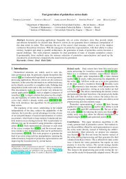
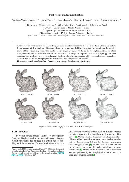
Fast stellar mesh simplificationANTÔNIO WILSON VIEIRA 1,2 , LUIZ VELHO 3 , HÉLIO LOPES 1 , GEOVAN TAVARES 1 AND THOMAS LEWINER 1,41 Department of Mathematics — Pontifícia Universidade Católica — Rio de Janeiro — Brazil2 CCET — Universidade de Montes Claros — Brazil3 Visgraf Project — IMPA — Rio de Janeiro — Brazil4 Géométrica Project — INRIA – Sophia Antipolis — France{awilson, lopes, tavares, tomlew}@mat.puc--rio.br. lvelho@impa.br.Abstract. This paper introduces Stellar Simplification, a fast implementation of the Four–Face Cluster algorithm.In our version of this mesh simplification scheme, we adopt a probabilistic heuristic that substitutes the priorityqueue of the original algorithm. This made our version, in average, 40% faster. In our implementation, we adopta very concise data structure which uses only two arrays of integers to represent the surface topology. We alsointroduce a new scheme to encode and decode the hierarchy of meshes generated by the simplification algorithm.This scheme can be used for progressive transmission and compression of meshes.Keywords: Mesh simplification. Geometry processing. Randomized algorithms.(a) level 2 – FFC (b) level 4 – FFC (c) level 8 – FFC (d) level 11 – FFC(e) level 2 – FS (f) level 4 – FS (g) level 8 – FS (h) level 11 – FSFigure 1: Bunny model simplified with 5098, 2628, 696 and 260 faces.1 IntroductionThe typical surface models handled by contemporaryComputer Graphics applications have millions of triangles.Mesh Simplification has emerged as a critical step for handlingsuch huge meshes. On one hand, there is an evi-Preprint MAT. 14/03, communicated on March 3 rd , 2003 to the Departmentof Mathematics, Pontifícia Universidade Católica — Rio de Janeiro, Brazil.The corresponding work was published in the proceedings of the Sibgrapi2003, pp. 27–34. IEEE Press, 2003.dent need for removing redundancies on meshes obtainedby surface reconstruction algorithms, such as the MarchingCubes [6]. On the other hand, meshes with a high level of detaileven without redundancies could be extremely expensivenot only for rendering, but also for storing or exchangingthem through the web [4]. In both cases, efficient simplificationprocess can get simpler models with lower computationalcosts [1]. Moreover, the hierarchical multi–resolutionstructure produced by our simplification can be used in awide range of applications [7].

A. Vieira, L. Velho, H. Lopes, G. Tavares and T. Lewiner 2Prior work. Many efficient mesh simplification methodsare based on local topological operators. The most commonis the Edge–Collapse, which consists in contracting the twovertices of an edge onto a unique vertex, eliminating its twoincident faces. The inverse of the Edge–Collapse operationis called Vertex–Split. Simplification schemes construct a sequenceof edges to be collapsed, resulting in a hierarchy ofmeshes of decreasing size. Traversing this sequence in a reverseorder, with Vertex–Split operations, it is possible to recoverdetails from the mesh of minimal size (base mesh). Althoughtopological tests can preserve the topology of the surfaceduring the simplification, its geometry will be distorted.To minimize this distortion, an energy function measuringthe quality of the mesh is used to guide the mesh simplification.An example of such function is the quadric error metric[3]. For those algorithms, the priority queue is a naturaldata structure to store the order of the edges to be simplified,since it allows a variety of operations (inclusion, removal ofthe largest, etc.) to be efficiently performed.Although the priority queue is efficient, it is necessary tobuild it before starting the simplification process. Moreover,at each step of the process a time is consumed not only to reprocessthe geometrical change for all edges involved in thelocal operation, but also to update their priority on the queue.In order to solve this problem, Wu and Kobbelt [11] presenteda technique called Multiple–Choice based on probabilisticoptimization where there is no use of a priority queue,but the edge to be contracted is chosen among d randomlyselected edges.Velho in [9] proposed a new method, called Four–Facecluster mesh simplification, which produces a sequence ofEdge–Weld operations intercalated with Edge–Flip operations.Edge–Weld and Edge–Flip are stellar operators [10].The Edge–Flip swaps an internal edge of a 2 face cluster.The Edge–Weld removes a valence 4 vertex from a four–facecluster and replaces it by the internal edge of a two–face cluster.Edge flips are required to change the valence of a vertexto 4. In this algorithm the energy functions are computed onvertices, and not on edges.Contributions. This work enhances the Four–Face Clustersalgorithm by substituting the priority queue by the Multiple-Choicetechnique. The result is an algorithm that isabout 40% faster than the original one and that requires lessmemory. We call the new algorithm Fast Stellar Simplification,because it is based on the stellar operators Edge–Weldand Edge–Flip. For a complete presentation of stellar operatorssee [10].We also introduce a new scheme to represent the hierarchyof meshes obtained during the process of simplification.In this scheme we adopt the Corner–Table data structure [8],which allows a concise and simple implementation of ournew algorithm. Finally, we propose two practical ways to encodeand decode, in a compressed way, the hierarchy of themulti–resolution mesh.Paper outline. Section 2 Corner–Table Data Structure describesthe Corner–Table data structure. Section 3 Local Operatorsand Topological Validation presents the topological operatorsthat will be used in our algorithm. Section 4 The Four–Face Cluster Method presents the original Four–Face clusteralgorithm. Section 5 The Fast Stellar Simplification Algorithmintroduces the Fast Stellar Simplification Algorithm basedon the multiple choice technique. Section 6 Simplification withMulti–Resolution presents the scheme to encode and decodethe hierarchy of the surfaces generated by the simplificationalgorithm. Finally, Section 7 Results shows some results andcomparison with the former Four–Face cluster algorithm.2 Corner–Table Data StructureBasic concepts. A simplex σ p of dimension p (p-simplex,for short) is the convex hull of p + 1 linearly independentpoints in R m , called its vertices. A p-simplex has p dimensionsand is composed of p + 1 simplices of dimension(p − 1), called faces. The set of 2, 1 and 0 dimensional simpliceswill be called, respectively, triangles, edges and vertices.If σ is a subsimplex of a simplex τ then they are saidto be incident to each other.A simplicial complex C is a finite set of simplices togetherwith all its subsimplices such that if σ k and τ p , k ≤ p belongto C, then either σ k and τ p meet at a subsimplex λ m , m ≤ k,or are completely disjoint. A triangle mesh is a simplicialcomplex whose simplices are at most dimension 2.Combinatorial manifolds. We will consider an orientabletriangulated combinatorial surface S. This is the general caseof manifold triangle meshes embedded in R 3 , but we are onlyconcerned with their connectivity, e.g., the triangle/vertexincidence and the triangle/triangle adjacency information.For more details in the following definitions, see [2].In a triangle mesh M, the star of a vertex v is a subset ofM composed by the union of simplices that are incident tov, and is denoted by star(v). . The link of a vertex v, denotedby link(v), is the frontier of star(v), or the union of 0 and 1simplices of star(v) that are not incident to v.. The Link ofan edge (u, v) are the opposite vertices by the edge (u, v).Definition 1 (combinatorial surface) A triangular meshM is a combinatorial surface if: Every edge in M is boundingeither one or two triangles and the link of a vertex in Mis homeomorphic either to an interval or to a circle.Corner–Table. The Corner–Table is a very concise datastructure for triangular meshes. It uses the concept of cornerto represent the association of a triangle with one of itsbounding vertices, or equivalently the association a trianglewith its bounding edge opposite to that corner: it may beviewed as a compact version of the half–edge representationof triangular meshes.In this data structure, the corners, the vertices and the trianglesare indexed by non–negative integers. Each triangle isrepresented by 3 consecutive corners that define its orientation.For example, corners 0, 1 and 2 correspond to the firstThe corresponding work was published in the proceedings of the Sibgrapi 2003, pp. 27–34. IEEE Press, 2003.

3 Fast stellar mesh simplificationtriangle, the corners 3, 4 and 5 correspond to the second triangleand so on. . . As a consequence, a corner with index cis associated with the triangle of index c.t = floor (c ÷ 3).The Corner–Table data structure represents the geometryof a surface by the association of each corner c with itsgeometrical vertex index V[c].Assuming a counter–clockwise orientation, for each cornerc, the next(c) and prev(c) corners on its triangle boundaryare obtained by the use of the following expressions:next(c) = 3c.t + (c + 1) mod 3, and prev(c) = 3c.t +(c + 2) mod 3.The edge–adjacency between the neighboring trianglesis represented by associating to each corner c, its oppositecorner O[c], which has the same opposite geometrical edge.This information is stored in two integer arrays, called the Vand O tables. Figure 2 shows an example of a Corner–Tablerepresentation for a tetrahedron.1100 2 03Figure 2: Tetrahedron exampleV[0] = 0 O[0] = 4V[1] = 1 O[1] = 9V[2] = 3 O[2] = 8V[3] = 1 O[3] = 10V[4] = 2 O[4] = 0V[5] = 3 O[5] = 7V[6] = 1 O[6] = 11V[7] = 0 O[7] = 5V[8] = 2 O[8] = 2V[9] = 2 O[9] = 1V[10] = 0 O[10] = 3V[11] = 3 O[11] = 63 Local Operators and Topological ValidationOur algorithm is based on two local topological operators:the Edge–Flip, and the Edge–Weld. In this section we willdescribe not only those two, but also the more classicalEdge–Collapse operator in order to compare them.Edge–Collapse: This operator consists in removing anedge e = (u, v), identifying its vertices to a unique vertex v.From a combinatorial viewpoint, this operator will remove1 vertex, 3 edges and 2 faces from original mesh, withoutchanging its Euler characteristic. From a geometric viewpoint,the new position of the vertex v can be computed withthe geometry around u and v. Let s and t be the vertices opustvFigure 3: Edge–Collapseposite to e = (u, v), which is the edge to be collapsed (seeFigure 3). Choosing edges according to the following linkstvcondition will guarantee the topological consistency of thisoperation [2] (see Figure 4).ust(a)vuFigure 4: Link ConditionLemma 2 (Link Condition) Let S be a combinatorial 2–manifold. The contraction of an edge e = (u, v) ∈ Spreserves the topology of S if and only if link(u)∩link(v) =link(e).Edge–Flip: This operation consists in transforming a two–face cluster into another two–face cluster by swapping itscommon edge. Let the edge e = (u, v) and s and t theabuc 4sc 3c 5c 2 c 1c 0tvcduFigure 5: Edge–Flipabstswt(b)c 1 c 4c 2 c 3c 0 c 5two vertices opposed to e (see Figure 5). The Edge–Flipoperation will replace e by (s, t), and replace the 2 trianglesincident to e by (u, s, t) and (v, t, s). In the Corner–Tabledata structure, each edge can be univocally represented byone of its opposite corners. This is used by the Algorithm 1to perform the Edge–Flip operation on the edge opposite tothe corner c 0 .Algorithm 1: Edge–Flip(c 0 )// Label incident cornersc 2 = prev(c 0 ); c 1 = next(c 0 );c 3 = O[c 0 ]; c 4 = next(c 3 ); c 5 = prev(c 3 );a = O[c 5 ]; b = O[c 2 ]; c = O[c 4 ]; d = O[c 1 ];// Label incident verticest = V [c 0 ]; v = V [c 1 ]; s = V [c 3 ];// Perform swapV [c 1 ] = s; V [c 3 ] = v; V [c 4 ] = s; V [c 5 ] = t;// Reset opposite cornersO[c 2 ] = c 3 ; O[c 0 ] = a; O[c 3 ] = c 2 ; O[c 4 ] = d;O[c 5 ] = c; O[a] = c 0 ; O[c] = c 5 ; O[d] = c 4 ;vvcdPreprint MAT. 14/03, communicated on March 3 rd , 2003 to the Department of Mathematics, Pontifícia Universidade Católica — Rio de Janeiro, Brazil.

A. Vieira, L. Velho, H. Lopes, G. Tavares and T. Lewiner 4asasc 3vsuvsuwb3c 4 c 5vcc c 2 0c 1tuc 4 c 5w c 0 c 2c 1btuvtsutsuFigure 6: Edge–WeldttFigure 7: Edge–Collapse decomposition.Edge–Weld. This operation consists in transforming afour–face cluster into a two–face cluster by removing its centralvertex. Consider a valence 4–vertex v, adjacent to thevertices s, t, w and u (see Figure 6). The star of v formsa four–face cluster. The Edge–Weld operation removes thevertex v and re–triangulates the quadrangle by splitting it.The dividing edge e can be either (w, u) or (s, t). The resultis a two–face cluster composed by the two faces incident toe.Theorem 3 Consider a combinatorial 2–manifold M, and avertex v of M with valence 4. With the notations of Figure 6,the removal of the vertex v by the Edge–Weld operationpreserves the topology of M if and only if there is no edge inM connecting w to u.Proof: Consider s, w, t and u, in this order, the vertices adjacentto v. Removing v is equivalent to an Edge–Collapseoperation on the edge e = (v, u). Therefore, the topologyof M is preserved if and only if the link condition is satisfied:link(v) ∩ link(u) = {s, t} = link(e). As {u, w} =link(v) \ link(e), this condition is valid if and only if w doesnot belong to link(u). This means that there is no edge connectingw to u.□Given a mesh represented by a Corner–Table, the Algorithm2 performs the removal of the vertex incident to thecorner c 0 :Algorithm 2: Edge–Weld(c 0 )// Assign incidencesc 1 = next(c 0 ); c 2 = prev(c 0 );c 4 = next(O[c 1 ]); c 5 = prev(O[c 1 ]);a = O[next(O[c 5 ])]; b = O[prev(O[c 2 ])];// Perform vertex removalV [c 0 ] = V [O[c 2 ]]; V [c 4 ] = V [c 0 ];// Reset opposite cornersO[c 5 ] = a; O[a] = c 5 ; O[b] = c 2 ; O[c 2 ] = b;Luiz Velho proved in [9] that the Edge–Collapse operationcan be decomposed into a sequence of Edge–Flips operations,followed by one Edge–Weld operation. The Figure 7illustrates this process.4 The Four–Face Cluster MethodThe Four–Face Cluster algorithm (FFC) is based on theEdge–Weld and Edge–Flip operators. Since the Edge–Collapseoperation is equivalent to a sequence of those stellaroperators, the Four–Face Cluster method can implement anEdge–Collapse based method. However, the stellar operationsare more flexible. In the case of the Edge–Collapse /Vertex–Split, there are many possible sequences of Edge–Flips leading to a final Edge–Weld. Therefore, the order ofthose Edges–Flips can be chosen to improve the quality ofthe mesh (for example improving aspect ratio or preservingdihedral angle), which is more tricky in the Edge–Collapseoperations. As a consequence, the Four–Face Cluster (FFC)algorithm is more flexible than Edge–Collapse based algorithms.Algorithm’s outline. The FFC algorithm constructs a hierarchyof meshes ( M 0 , M 1 , . . . , M n) with a decreasingnumber of elements (vertices, edges and faces). In this hierarchy,surface M 0 is the original surface M, and each surfaceM j , j = 1 . . . n, corresponds to the level of detail jof M. We will now describe how we obtain such levels ofresolutions.In the initialization step for each level of detail j, all thevertices of M j−1 are marked as valid for removal. Then,we select a marked vertex v to be removed from the surfaceM j−1 . When the valence of the vertex v is not 4, we applya sequence of Edge–Flip operations to bring its valence to4. The four vertices on the star of the modified vertex v arethen unmarked. They will not be valid for further removaluntil the next level of detail j + 1. Next, we remove thevalence 4 vertex v using an Edge–Weld operation. Figure 7illustrates this sequence of operations. When all the verticesare unmarked, the resulting surface M j corresponds to levelof detail j inside the hierarchy of surfaces. On entering thenext step, we mark all the remaining vertices of M j in orderto create M j+1 and so on.Quadric Error Metric. Each local simplification introducesa geometric error between the surfaces M j and M j+1 .This cost is computed in the original FFC algorithm using theQEM [3], as follow.The corresponding work was published in the proceedings of the Sibgrapi 2003, pp. 27–34. IEEE Press, 2003.

5 Fast stellar mesh simplificationLet v be a vertex of M j , and f i ∈ star(v) a face incidentto v. Let a i be the area of f i and p i = (n x , n y , n z , d) theplane supporting f i . The fundamental error quadric Q i isdefined in [3] by:Q i = p i p T i =⎛⎜⎝⎞n 2 x n x n y n x n z n x dn x n y n 2 y n y n z n y d⎟n x n z n y n z n 2 z n z d ⎠n x d n y d n z d d 2It can be used to compute the squared distance d (w) of apoint w to the plane p i :d i (w) = w T ( p i p T )i w = w T Q i wGarland and Heckbert compute their quadric error metric byadding all of those distances d i (w) for all face f i .Simplification criterion. The FFC algorithm assigns aquadric Q v to each vertex v of the mesh, which is computedas the weighted sum of the quadrics Q i associated with eachface f i incident to v:Q v = ∑ a i Q iWe compute the error introduced by removing a vertex vfrom the mesh, considering each Edge–Flip and Edge–Weldcosts, by [9]:E (v) = αC (v) + βS (v)This cost balances the vertex removal distortion C (v) andthe swap distortion S (v). In our implementation, we choseα = 0.75 and β = 0.25. The cost C (v) of removing a vertexv of valence 4 is defined as:C (v) = min { u T (Q v + Q u ) u, u ∈ link(v) }The cost S (v) is the sum of the cost of Edge–Flips inStar(v) used to bring v to valence 4. To compute thiscost, we compute the sequence of independent Edge–Flips,minimizing the aspect ratio [12] and trying to preserve thedihedral angle.Implementation. The original implementation used a priorityqueue, which requires computing the costs of all verticesbefore beginning the simplification. Moreover, at eachsimplification step, we need to re–compute the cost of all verticesinvolved in the local operation. With a priority queue,we would have to update corresponding priorities. The Algorithm3 gives the pseudo–code for the Four–Face ClusterSimplification Algorithm introduced in [9]. It generatesn levels of resolution of a given mesh M.Algorithm 3: SimplifyFFC(M, n)assign quadrics;for all(v ∈ M) docompute E (v)for (j = 1 to n) domark all vertices as valid for removalinsert all vertices in the priority queuewhile (queue is not empty) doget v from queueif (v marked) thenperform edge swaps to bring v to valence 4unmark the vertices w ∈ link(v)remove vertex (v)re–compute the errors Q u and Q wupdate queue for w ∈ link (u) ∪ link (w)5 The Fast Stellar Simplification AlgorithmAn alternative to simplification methods based on priorityqueue was presented by Wu and Kobbelt in [11]. Theypropose, instead of using the priority queue, to choose theelement to be simplified inside a reduced, randomly selectedset of d elements. This probabilistic optimization strategy ismotivated by the fact that when simplifying high resolutionmeshes, most of the vertices will be removed anyway. As aconsequence, it would not be necessary to choose a vertexwith lower cost among all possible candidates at each simplificationstep.The basic idea of this Multiple–Choice technique is toobtain a small random subset of d edges to be collapsed,say d = 8, and perform the collapse for the edge with thelower cost among them. Our implementation is an adaptationof this idea, since we compute costs on vertices and not onedges. We obtain a random subset of vertices to be simplifiedand perform the simplification for the vertex with the lowercost of this set. This strategy leads to a good choice of thevertex to be simplified, except for a rare probability that alld random vertices were among the vertices that should notbe removed. Assuming that we simplify a 3D model down to5% of its original complexity, we hope that the resulting (notremoved) vertices will have high costs. The probability ofchoosing one of the high–cost vertices on a random subset ofd = 8 vertices is actually small enough: ( 5100) 8≈ 4×10 −11 .Using this technique we do not need to sort the verticesby their cost, avoiding the expansive use of a priority queue.Since, at each randomly selected subset the costs of the dvertices will be recomputed, it is also not necessary to re–compute the cost for the vertices on the neighborhood ofthe removed vertex. This allows a simpler implementationand improves the algorithm’s performance. The Algorithm 4shows the pseudo–code to generate n levels of resolution fora mesh M using this process:Preprint MAT. 14/03, communicated on March 3 rd , 2003 to the Department of Mathematics, Pontifícia Universidade Católica — Rio de Janeiro, Brazil.

A. Vieira, L. Velho, H. Lopes, G. Tavares and T. Lewiner 6Algorithm 4: SimplifyFS(M, n)assign quadrics;for (j = 1 to n) domark vertices as valid for removalwhile (exist a valid vertex) dofor (i = 1 to 8) dov i =valid random vertexif E(v i ) < E(v) then v = v iperform edge swaps to bring v to valence 4unmark the vertices w ∈ link(v)remove vertex (v)re–compute quadrics Q u and Q wWhen the number of valid vertices is less then 8, one ormore vertices can be selected more than once in order toremove all valid vertices.6 Simplification with Multi–ResolutionOne objective of this section is to introduce two strategiesto encode the hierarchy of meshes ( M 0 , M 1 , .., M n) generatedby our Fast Stellar simplification algorithm: the paralleland the sequential encoding. The main difference betweenthose two strategies relies in the type of hierarchical structurethey produce. The parallel encoding produces a multi–resolution mesh with separated levels of details, whose resolutionchanges globally on each level. The sequential encodingproduces a progressive mesh, whose resolution changeslocally inside each level.Multi–resolution representation. The Corner–Table datastructure uses only two arrays (O and V) of integers torepresent the surface topology and a third array (G) to storethe geometry of the mesh. In order to represent the hierarchyof surfaces, in our implementation we adopt the followingstrategy. The connectivity of the surface M j is representedby the arrays O j and V j , while its geometry uses the originalarray G for all levels of detail, since we do not modifythe indices of the vertices during the simplification process.Therefore, in order to change from one level to another, wesimply allocate the arrays O and V corresponding to thedesired level.Parallel Encoding. This strategy produces a multi–resolutionmesh whose resolution changes globally at each level.Parallel encoding is useful when the user wants to movefrom one level of resolution to another. In such application,we could allocate only the memory necessary to representthe surface of a certain level. Thus, we simply need toencode the surface M j . We implemented this encoding in acompressed manner (with less than 2 bits per triangle) usingthe Edgebreaker compression scheme.We used Edgebreaker because there is a very concise andsimple implementation of this compression scheme for surfaceswith handles using the Corner–Table data structure [5].We modify this implementation by adding a fourth attributeto vertex geometry, its index on the G table of the originalsurface. Maintaining these indices for the vertices at eachlevel of detail enable us to interchange the use of paralleland sequential encoding. For example, in the application wecan move directly to the level 5 of resolution using the parallelencoding, and then in a progressive way return to thelevel 4 by the use of the sequential encoding.Sequential Encoding. In the sequential case, we encodeeach stellar operation: at each vertex simplification we storethe history of the Edge–Flips and Edge–Welds operations.This strategy is similar to the Progressive Mesh encoding [4],which encodes the history of Edge–Collapse operations fortheir simplification algorithm. The main idea of this encodingis to obtain a refinement process by reading in the reverseorder the history of stellar operations performed by the FastStellar simplification algorithm.In the sequential encoding, we store a string of integers torepresent the sequence of operations performed on each vertexsimplification. Figure 8 illustrates a vertex simplificationwith the encoding of the corresponding operations. Let call v1 26 7 3541 26 7 3541 26 7 3541 26 31 14 1463-7Figure 8: Encoding of a vertex simplificationthe vertex to be removed, and e = (u, v) ∈ star(v) an edgeto be swapped. Since each e has v as extremity, we encodeonly the index of u to represent an Edge–Flip operation. TheEdge–Weld operation is encoded by 3 integers 2 integers forencoding the resulting edge of the vertex removal and 1 integerto encode the original index of the removed vertex.In order to interchange the parallel encoding with the sequentialencoding, we write each level of detail in a separatedfile. As a consequence, we start the progressive refinementprocess at any level of detail obtained by the simplification.In the Progressive Mesh [4], the starting surface for refinementis restricted to be the base mesh.7 ResultsThe results presented in [11] shows that the performancesof mesh simplification algorithms using the Multiple–Choicetechnique are 2.5 times faster than using a priority queue,with similar outputs. Furthermore, the Multiple–Choicetechnique leads to a simpler implementation, since there isno need for a priority queue construction or of re–computationat each simplification step. Similarly, the experimentsbelow show that the Fast Stellar simplification is 40% fasterthan the original Four–Face Cluster algorithm.Table 1 shows the running time of each routine duringthe simplification, using the Four–Face Cluster (FFC) andFast Stellar (FS) algorithms. Table 2 shows the total runningtime comparison (in sec) for simplifying some models. No-54The corresponding work was published in the proceedings of the Sibgrapi 2003, pp. 27–34. IEEE Press, 2003.

7 Fast stellar mesh simplificationFFCFSOperation t(s) % t(s) %Assign Quadrics 0.110 1.26 0.110 1.95Compute E (v) 7.880 90.51 4.930 87.54Update Queue 0.360 4.14 – –Choose d random v – – 0.340 6.04Edge Swaps 0.165 1.90 0.088 1.56Vertex Removal 0.170 1.95 0.141 2.50Recompute Q u /Q w 0.021 0.24 0.023 0.41Total 8.706 100 5.632 100Table 1: algorithm’s steps comparison.# Triangles Running time RatioModel Input Output FFC FS ffc/fsBunny 9672 260 7.320 4.130 1.77Cow 5804 202 4.680 2.780 1.68Terrain 5708 190 4.520 2.690 1.68Torus 14144 344 9.100 5.110 1.78Table 2: Total time comparison.tice that the total time for the Stanford’s Bunny model in Table1 is greater then in Table 2 because of we did some moremeasures of time spent by each routine. Figure 9 comparesthe absolute maximum geometric error, based on QEM, introducedfor the Bunny model in various levels of details bythe two different algorithms.In Figure 10 we present two examples of models to visuallycompare the two algorithms. Notice that, as in [11], theresults got in both methods are similar. For the first example,we chose the Stanford’s Bunny model. Figure 1 showsthe levels of detail 2, 4, 8 and 11 obtained using the FFC andthe FS. Figure 11 shows the simplification of cow model, oursecond example. We show in this figure the levels of detail6, 8, 10 and 12 obtained using both algorithms.8 Conclusions and Future worksIn this paper we presented the Fast Stellar simplificationalgorithm, which is a fast implementation for the Four–Face cluster algorithm. We adopted the Corner–Table datastructure to represent the surface, which shows to be verysuitable not only for the stellar operators’ implementationbut also for the encoding. We pointed out the conditionsto safely apply the Edge–Weld and Edge–Flip operators.We also proposed two strategies to encode and decode thehierarchy of surfaces generated by the simplification.We plan to continue this work in three directions. First,we will try to create an efficient compression scheme for thesequential encoding. Second, we intend to use this simplificationalgorithm to obtain a parameterization scheme forsurfaces, which is a very active area of research in ComputerGraphics. Finally, we will investigate a hardware implementationof this algorithm taking advantage of the simplicity ofthe Corner–Table data structure.References[1] P. Cignoni, C. Montani and R. Scopigno. A comparisonof mesh simplification algorithms. Computers & Graphics,22(1):37–54, 1998.[2] H. Edelsbrunner. Geometry and topology for mesh generation.Cambridge Monographs on Applied and ComputationalMathematics, 2002.[3] M. Garland and P. S. Heckbert. Surface simplificationusing quadric error metrics. Computers & Graphics,31:209–216, 1997.[4] H. Hoppe. Progressive meshes. In Siggraph, pages 99–108, New Orleans, Aug. 1996. ACM.[5] H. Lopes, J. Rossignac, A. Safonova, A. Szymczak andG. Tavares. Edgebreaker: a simple compression for surfaceswith handles. In C. Hoffman and W. Bronsvort, editors,Solid Modeling and Applications, pages 289–296,Saarbrücken, Germany, 2002. ACM.[6] W. E. Lorensen and H. E. Cline. Marching Cubes: ahigh resolution 3D surface construction algorithm. InSiggraph, volume 21, pages 163–169. ACM, 1987.[7] E. Puppo and R. Scopigno. Simplification, LOD andmultireolution – principles and applications. In EurographicsTutorial, page PS97 TN4, 1997.[8] J. Rossignac, A. Safonova and A. Szymczak. 3S compressionmade simple: Edgebreaker on a corner–table.In Shape Modeling International, pages 278–283. IEEE,2001.Figure 9: Geometric error comparison[9] L. Velho. Mesh simplification using four–face clusters.In Shape Modeling International, pages 200–208. IEEE,2001.Preprint MAT. 14/03, communicated on March 3 rd , 2003 to the Department of Mathematics, Pontifícia Universidade Católica — Rio de Janeiro, Brazil.

A. Vieira, L. Velho, H. Lopes, G. Tavares and T. Lewiner 8Figure 10: Models used in the examples: Bunny model (9672 faces) and Cow model (5804 faces).(a) level 6 – FFC (b) level 8 – FFC (c) level 10 – FFC (d) level 12 – FFC(e) level 6 – FS (f) level 8 – FS (g) level 10 – FS (h) level 12 – FSFigure 11: Cow model simplified with 1182, 640, 382 and 202 faces.[10] L. Velho, H. Lopes and G. Tavares. Mesh ops. Technicalreport, Department of Mathematics, PUC–Rio, 2003.[11] J. Wu and L. Kobbelt. Fast mesh decimation bymultiple–choice techniques. In Vision, Modeling and Visualization,pages 241–248. IOS Press, 2002.[12] A. Guéziec, F. Bossen, G. Taubin and C. Silva. Efficientcompression of non–manifold polygonal meshes. ComputationalGeometry: Theory and Applications, 14(1–3):137–166, 1999.The corresponding work was published in the proceedings of the Sibgrapi 2003, pp. 27–34. IEEE Press, 2003.