A study of time integration schemes for the numerical modelling of ...

INTERNATIONAL JOURNAL FOR NUMERICAL METHODS IN FLUIDSInt. J. Numer. Meth. Fluids (in press)Published online in Wiley InterScience (www.interscience.wiley.com). DOI: 10.1002/d.981A study of time integration schemes for the numericalmodelling of free surface owsAhamadi Malidi § , Steven Dufour ∗; †; ‡ and Donatien N’dri §Departement de mathematiques et de genie industriel; Ecole Polytechnique de Montreal; C.P. 6079;succ. Centre-ville; Montreal (Quebec) Canada, H3C 3A7SUMMARYA semi-discrete nite element methodology for the modelling of transient free surface ows in thecontext of Eulerian interface capturing is proposed. The focus of this study is put on the choice of anappropriate time integration strategy for the accurate modelling of the dynamics of free surfaces andof interfacial physics. It is composed of an adaptive time integration scheme for the Navier–Stokesequations, and of the implicit midpoint rule for the transport equation of the Eulerian marker variable.The adaptive scheme allows the automatic determination of a time-step size that follows the physics ofthe problem under study, which facilitates the accurate modelling of sti free surface ows. It is shownthat the implicit midpoint rule reduces mass loss for each uid. Various free surface ow problems arestudied to verify and validate the proposed time integration strategy. Copyright ? 2005 John Wiley &Sons, Ltd.KEY WORDS:free surface ows; interface capturing; time integration schemes; nite element methods1. INTRODUCTIONThe numerical modelling of free surface ows is a challenging problem. Since the positionof the interface separating the uids is a priori unknown, specic algorithms must be usedto determine its position. Several strategies are described in the literature for performing∗ Correspondence to: Steven Dufour, Departement de mathematiques et de genie industriel, Ecole Polytechnique deMontreal, C.P. 6079, succ. Centre-ville, Montreal (Quebec) Canada H3C 3A7.† E-mail: steven.dufour@polymtl.ca‡ Assistant Professor.§ Research Associate.Contract=grant sponsor: Auto21 Network of Centres of Excellence of CanadaContract=grant sponsor: Natural Sciences and Engineering Research Council of CanadaContract=grant sponsor: Fonds quebecois de la recherche sur la nature et les technologiesReceived 1 December 2004Revised 18 March 2005Copyright ? 2005 John Wiley & Sons, Ltd. Accepted 21 March 2005

A. MALIDI, S. DUFOUR AND D. N’DRIcomputer simulations of multiuid ows [1]. In this study, we are particularly interested ina family of methods based on a marker variable that is used to identify the region occupiedby each uid. The zero thickness interface is traded for a transition zone of the marker.This variable is then transported by the velocity eld of each uid, by solving a transportequation of the marker on a xed grid. This Eulerian approach, which is also known asfree surface capturing, is popular for modelling complex multiuid ows. Among the mostpopular free surface capturing methods we can mention the volume of uid method [2],the level set method [3], and the pseudo-concentration method [4], to name a few. Thisapproach is better suited for modelling the evolution of free surfaces submitted to largeand complex deformations. Modelling multiple interface ows is not a complicated matter,since the interface is not treated as an explicit computational entity. Free surface splittingand reconnection are handled implicitly. However, this strategy is known to be lessaccurate if the numerical strategy is not well chosen. This is due to the uncertaintyinherent in the use of the region of transition of the marker variable to locate the free surface,which makes it impossible to impose interfacial boundary conditions explicitly. Freesurface capturing methods are also known to suer from numerical diusion or oscillations[5]. This results in the deformation of the region of transition of the markervariable, and therefore to mass-conservation problems and to an inaccurate modelling ofinterfacial physics. It is therefore important to choose the right numerical strategy inorder to perform an accurate transport of the free surfaces, and to conserve mass foreach uid.Several components in a numerical methodology inuence the accuracy of a free surfacecapturing strategy. An inaccurate discretization may lead to an imbalance between the viscousforces and the capillary forces, which will translate into numerical instabilities [6]. It is wellknown that a ‘good’ mesh will provide an accurate discretization of the variables of theproblem [6]. We also observe that the elliptic solvers introduce non-physical oscillations ordiusion when the solution of a partial dierential equation contains a discontinuity or anabrupt variation [7]. Finally, the choice of an appropriate time integration scheme, to discretizethe transient term of the equations, is important to help conserve mass for each uid. To ourknowledge, we do not know of a study relating the discretization in time to mass-conservationproblems and interfacial instabilities when modelling free surface ows using an Eulerianapproach.Authors studying multiuid ows use various time integration schemes. Examples are: thebackward Euler scheme for mold lling problems [8]; the trapezoid rule (TR) for sloshingproblems [9]; and the backward dierentiation formula (BDF) (Gear scheme) for dropsdynamics problems [10] to name a few. But these studies do not mention the reasons forthese choices. We are proposing to discuss various strategies for the discretization of thetransient term of the partial dierential equations involved in the modelling of free surfaceows in an Eulerian context.After introducing the semi-discrete nite element methodology used for modelling free surfaceows using interface capturing, we rst look at the time discretization of theNavier–Stokes equations, which is important for modelling sti free surface ow problems.We then study the inuence of the discretization of the transient term of the transport equationon mass conservation. We nally propose an overall time integration strategy for studyingfree surface ows. Various free surface ow problems are studied to verify and validate theproposed numerical strategy.Copyright ? 2005 John Wiley & Sons, Ltd.Int. J. Numer. Meth. Fluids (in press)

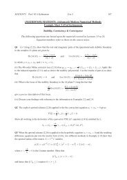
A STUDY OF TIME INTEGRATION SCHEMES FOR MODELLING FREE SURFACE FLOWS2. MODELLING OF THE PROBLEMConsider the free surface ow problem illustrated in Figure 1. The region occupied by therst uid is denoted 1 . The second uid occupies the region 2 , and since the uids areimmiscible, 1 ∩ 2 = ∅. The computational domain can therefore be dened as = 1 ∪ 2 .The interface separating the two uids is denoted by S. The unit normal to the interface isdenoted n S .The ow of each uid is modelled using the equations expressing conservation of massand momentum. Therefore, the equationsand∇ · u = 0 (1) @u + (u · ∇)u = ∇ · (2)@tmust be solved for uids 1 and 2, i.e. on 1 and 2 , respectively, where =−pI + is the Cauchy stress tensor, and the density of the uid is denoted . The extra-stress tensor is related to the velocity eld by the relation =2˙(u)where is the viscosity of the uid, and the rate-of-strain tensor ˙ is dened by˙(u)= 1 2 (∇u +(∇u)T )The dependent variables of the problem will therefore be denoted u 1 and u 2 for the velocityeld of uids 1 and 2, and the pressure of the uids will be denoted p 1 and p 2 .Boundary conditions can either be of the essential type (Dirichlet boundary conditions):u i = u @ or of the natural type (Neumann boundary conditions): i · n = t @ , where i =1; 2inour case. The conditions at the interface S are [1]: the continuity of normal velocitiesu 1 · n S = u 2 · n S = u S · n Su 2nΩ 1Ω 2Figure 1. A free surface ow problem.Copyright ? 2005 John Wiley & Sons, Ltd.Int. J. Numer. Meth. Fluids (in press)

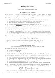
A STUDY OF TIME INTEGRATION SCHEMES FOR MODELLING FREE SURFACE FLOWSis used to discretize the transport equation (3). A quadratic element is used to discretize thepseudo-concentration. The stabilization parameter is given by h=2‖u‖, where h is the localmesh size.The continuum surface force model [12] is used to include the inuence of surface tensionin the numerical model. Surface tension is considered as a volume force dened in the smoothregion of transition of the Eulerian marker variable. Formally, the surface capillary forcef S = n S S is written as a volume force f V = (F)∇F, dened in the region of transitionof F. The Dirac delta function S , dened on the interface S, is approximated numericallyin the region of transition of F using ‖∇F‖, and the curvature is approximated using( ) ∇F =−∇ · n S ≈−∇ ·‖∇F‖The capillary force f V is included in the Navier–Stokes equations (2) to yield @u@t + (u · ∇)u = ∇ · + f V (5)4. TIME INTEGRATION SCHEMES FOR THE NAVIER–STOKES EQUATIONS4.1. Motivation: Laplace’s problemAn accurate discretization of the velocity eld of the uids is important for an accurate advectionof the pseudo-concentration (cf. Equation (3)). A well-known free surface ow problem,for which an inaccurate discretization of the transient term of the Navier–Stokes equations canbe problematic, is Laplace’s problem. The problem consists of a ‘two-dimensional’ drop ofuid of an arbitrary shape, an ellipse for example, in another uid at rest. The capillary forcebetween the two uids induces a ow which makes the drop reach a topology that minimizesenergy, i.e. a circle in two dimensions. The curvature of the steady-state drop and the jumpin pressure should verify Laplace’s law,p 1 − p 2 = (6)This problem is popular for verifying numerical surface tension models in simulation codes.Despite its simplicity, Laplace’s problem is numerically challenging. It is well documentedin References [13–18] that if the numerical strategy is not well chosen, numericallyinduced parasitic currents will appear in the vicinity of the free surface when ‖u‖ →0 (cf.Figure 2(a)). This leads to an inaccurate discretization of the jump in pressure at the freesurface (cf. Figure 2(b)), and eventually to a ow that does not reach a steady-state. Severalhypotheses are brought forward in the literature in order to explain this phenomenon and tond a cure.Kothe et al. [14] convolve the marker variable F with various smooth kernels to obtaina mollied colour function ˜F. This leads to a more accurate computation of the unit normalto the free surface n S and of the curvature , which in turn reduces parasitic currents. Otherauthors have improved the numerical discretization they were using in order to obtain a moreaccurate modelling of interfacial physics. This is the case of Popinet and Zaleski [15] whouse higher accuracy discretizations of the Lagrangian representation of the free surface, andof the pressure, which leads to a reduction of parasitic currents. In a similar fashion, theCopyright ? 2005 John Wiley & Sons, Ltd.Int. J. Numer. Meth. Fluids (in press)

A. MALIDI, S. DUFOUR AND D. N’DRIFigure 2. Numerical instabilities in modelling Laplace’s problem: (a) parasiticcurrents; and (b) pressure contours.PROST algorithm [17] was also devised to eliminate the spurious currents problem. In thisalgorithm, free surface capturing is performed with the VOF (volume of uid) technique, usinga least square t of a quadratic surface to the colour function for each interface cell and itsneighbours. The authors also implemented a higher-order advection scheme for the transportequation of the colour function. Hou et al. [19] rather consider Laplace’s problem as a stiproblem. They devised a numerical procedure based on the boundary integral formulation toremove the stiness due to surface tension. The numerical results found in these referencesshow that parasitic currents are in fact reduced, but it is not clear if the steady-state is reached.We have found that several aspects of these studies are important [20]. In particular, thefact that this problem is sti is often overlooked, and we think, like Hou et al. [19], that this isthe key to the accurate modelling of Laplace’s problem. This led us to develop a methodologyto tackle sti free surface ow problems through the use of a time integration strategy whichincludes an adaptive scheme for the transient term of the Navier–Stokes equations. Thisstrategy will allow us to modify the size of the time discretization in order to maintain thebalance between the viscous forces and the capillary forces when approaching steady-state.Our hypothesis is that such a scheme will allow us to reach the steady-state of Laplace’sproblem with no parasitic currents at the free surface.4.2. Adaptive time integration schemeAdaptive time integration schemes for the Navier–Stokes equations are not new in thecomputational science literature (cf. Reference [21] for details). They allow the automaticcomputation of an ‘optimal’ time-step size t n at every time step, in order to adapt the timediscretization to follow the physics of the modelled problem. This strategy is a common practicefor discretizing spatial variables. It is dicult to explain why it is not more popular inthe CFD literature for the temporal variable. It is particularly absent from the free surfaceow modelling literature.The most popular adaptive time integration scheme is the adaptive trapezoid rule (ATR).Even if this scheme is devised to compute the appropriate time-step size in order to avoidthe oscillations often seen with the standard TR, the ATR scheme can still exhibit wigglesCopyright ? 2005 John Wiley & Sons, Ltd.Int. J. Numer. Meth. Fluids (in press)

A STUDY OF TIME INTEGRATION SCHEMES FOR MODELLING FREE SURFACE FLOWSin some cases [21]. This is why we choose to use an adaptive backward dierentiationformulae (ABDF), which is based on the constant-time-step size second-order accurate BDF,also known as Gear scheme. This choice is justied by the fact that the BDF scheme isknown to damp oscillatory solutions.The nite element discretization of velocity and pressure,∑u(x)= 7 ∑u i ’ i (x) and p(x)= 3 p i i (x)i=1where ’ i (x) and i (x) are the nite element interpolation functions of the Crouzeix–Raviartelement and the u i and the p i are the degrees of freedom of velocity and pressure on anelement, are introduced in the elementary linearized weak forms of the conservation of mass(1) and momentum (2) equations, to yield an algebraic system of equations of the form (seeReference [22] for details)[ ] ⎡ ⎤M 0˙ [Ũ A BT] ⎡ ⎤ ⎡ ⎤Ũ ˜F⎣ ⎦ + ⎣ ⎦ = ⎣ ⎦0 0 ˜P˙ B 0 ˜P ˜0The vector Ũ contains the degrees of freedom in velocity, ˜P contains the degrees of freedomin pressure, M is the mass matrix of the transient term, A is the viscous term matrix andB is the discrete divergence matrix. But since we are using Uzawa’s algorithm to enforcethe incompressibility constraint, as described in Section 3, this linear system of equationsreduces toMŨ ˙ + A r Ũ = F r (7)(cf. Reference [11] for details). We therefore perform transient error control only on thedegrees of freedom in velocity. The degrees of freedom in pressure will be updated byUzawa’s algorithm.Following the development of Gresho et al. [21], we implemented an ABDF scheme forthe discretization of the Navier–Stokes equations. Based on the second-order accurate BDF,the variable-time-step size BDF scheme can be expressed asŨ˙n+1 = (2+(t n−1=t n ))Ũ n+1 − (2+(t n−1 =t n )+(t n =t n−1 ))Ũ n +(t n =t n−1 )Ũ n−1(8)t n +t n−1Using Taylor’s expansions:::ũ(t n±1 )=ũ(t n ± t n ) ≈ Ũ n±1 = Ũ n ± t ˙nŨn + 1 2 t2 nŨ n ± 1 6 t3 n Ũ n +O(tn) 4 (9)in (8), we nd the local truncation error of this variable-time-step size BDF scheme to beŨ n+1 − ũ(t n+1 )= (t n +t n−1 ) 2t n (2t n +t n−1 )t 3 n6:::Ũ ni=1+ O(t 4 ) (10)In order to be able to determine the next time-step size t n+1 , we need to express the localtruncation error of the ABDF scheme in term of Ũ n+1 . We rst need some kind of ‘cheap’Copyright ? 2005 John Wiley & Sons, Ltd.Int. J. Numer. Meth. Fluids (in press)

A. MALIDI, S. DUFOUR AND D. N’DRI:::predictor scheme with a local truncation error which is also in tn3 Ũ n . The variable-time-stepsize explicit midpoint rule is such a candidate:(Ũ p n+1 = Ũ n + 1+ t ) ( ) 2nt ˙ tnnŨn − (Ũ n − Ũ n−1 ) (11)t n−1 t n−1with a local truncation error ofŨ p n+1 − ũ(t n+1)=−:::(1+ t )n t3nt n−1 6Ũ n+ O(t 4 ) (12)which can again be obtained by using (9) in (11).We can now express the local truncation error of the ABDF scheme in terms of only Ũ n+1 ,Ũ p n+1 and t n. Subtracting Equation (12) from Equation (10), we obtainwhich can be written as:::[Ũ n+1 − Ũ p n+1 ≈ (tn +t n−1 ) 2 (t n (2t n +t n−1 ) + 1+ t )]n t3nt n−1 6t 3 n6:::Ũ nin order to rewrite expression (10) as≈ (Ũ n+1 − Ũ p n+1 ) /[ (tn +t n−1 ) 2t n (2t n +t n−1 ) + (1+ t nt n−1)]Ũ n+1 − ũ(t n+1 ) ≈ (t n+t n−1 ) 2 {/[(Ũ n+1 −Ũ p n+1t n (2t n +t n−1 )) (tn +t n−1 ) 2t n (2t n +t n−1 ) + t ]}n+1t n−1After simplifying this expression, we can express the local truncation error of the ABDFscheme, which will now be denoted ˜d n ,asŨ n˜d n = (1+(t n−1=t n ))(Ũ n+1 − Ũ p n+1 )2+(t n−1 =t n ) + 2(t n =t n−1 )(13)The new time-step size is then obtained by rst observing that the local truncation error(10) of (8) gives us:˜d n+1= Ũn+2 − ũ(t n+2 )˜d nU n+1 − ũ(t n+1 ) ≈ t3 n+1:::Ũ n+1:::tn3 Ũ n( ) 3 tn+1≈(14)t nSince we want to control the size of the local truncation error at the next time step, i.e.‖˜d n+1 ‖¡ (15)Copyright ? 2005 John Wiley & Sons, Ltd.Int. J. Numer. Meth. Fluids (in press)

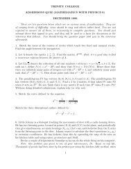
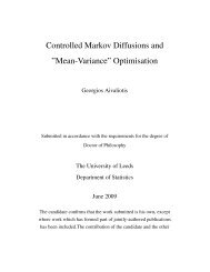
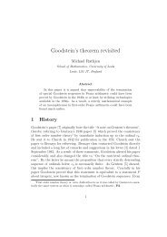
A STUDY OF TIME INTEGRATION SCHEMES FOR MODELLING FREE SURFACE FLOWS1.5Time History for the Von Karman ProblemTime-Step Sizes10.500 50 100 150TimeFigure 5. Time-step sizes computed by the ABDF scheme for the Von Karman problem. =5:80. The wavelength of their simulations was =5:32. Based on our results, we nd thesame period and wavelength.Finally, Figure 6 illustrates plots of various quantities at t = t ref , in order to compare qualitativelyour results with the ones of Engelman and Jamnia. We can again see that our guresare very similar to the ones of the benchmark paper.4.4. Laplace’s problem revisitedLaplace’s problem will now be studied using the ABDF time integration scheme for theNavier–Stokes equations. The discretization of the transient term of the transport equation (3),which is not a problem in this case, will be discussed in the next section.Let us consider a ‘2-D’ drop of uid of area 4 in a geometry with dimensions [−3; 3] ×[−3; 3]. As an example, the initial drop can have the shape of an ellipse described byy = ±B √ 1 − (x 2 =L 2 ), such that LB = 4, where L and B are the longest and shortest semiaxesof the ellipse. The uids are initially at rest, with same density and viscosity. Let ussuppose that the surface tension coecient between the uids is =2. If L ≠ B, the capillaryforce will generate a ow which will deform the drop until it reaches the shape of a circle ofradius 2 in this case. According to Laplace’s law (6), we should observe a jump in pressureof p 1 − p 2 =1.Using the methodology described in Section 3 with the ABDF scheme, and with a structuredmesh containing 140 × 140 elements, the numerical modelling of Laplace’s problem gives usthe time-step sizes illustrated in Figure 7. We observe a behaviour similar to the one illustratedin Figure 5 for the Von Karman problem, i.e. larger time-step sizes during the transient phaseof the simulation, and smaller time-step sizes when the drop is reaching its steady-state shape.We, however, do not have the apparent ‘noise’ observed before, but we still observe smallCopyright ? 2005 John Wiley & Sons, Ltd.Int. J. Numer. Meth. Fluids (in press)

A. MALIDI, S. DUFOUR AND D. N’DRIFigure 6. Plots at t = t ref for the Von Karman vortex street problem: (a) horizontal velocity component;(b) vertical velocity component; and (c) pressure.variations of t n . This can be explained by the fact that when the drop reaches its steadystateshape, we still observe very small deformations of the free surface that are captured bythe transient error estimator. Figure 8 illustrates the time evolution of the jump in pressure.The fact that (p 1 − p 2 ) → 1 is an indication that the steady-state is reached. Streamlines arealso useful to determine if the steady-state of a free surface ow is reached. It can be seenin Figure 9(a) that the streamlines do not cross the free surface, which is another goodindication that the numerical strategy allows us to reach the steady-state of this problem, withno parasitic currents. Another indication that the surface tension-driven ow simulation isperformed accurately is the smooth transition of pressure, with no irregularities, as illustratedin Figure 9(b).Copyright ? 2005 John Wiley & Sons, Ltd.Int. J. Numer. Meth. Fluids (in press)

A STUDY OF TIME INTEGRATION SCHEMES FOR MODELLING FREE SURFACE FLOWS0.16 Laplace’s Problem0.140.12Time-Step Sizes0.10.080.060.040.0200 50 100 150 200 250 300Time StepsFigure 7. Time-step sizes computed by the ABDF scheme for Laplace’s problem.Laplace’s Problemreference∆ p1Pressure Jump00 100 200 300 400Time StepsFigure 8. Time evolution of the jump in pressure for Laplace’s problem.Copyright ? 2005 John Wiley & Sons, Ltd.Int. J. Numer. Meth. Fluids (in press)

A. MALIDI, S. DUFOUR AND D. N’DRI(a)(b)Figure 9. Steady-state of Laplace’s problem: (a) streamlines; and (b) pressure contours.5. TIME INTEGRATION SCHEMES FOR THE TRANSPORT EQUATION5.1. Motivation: the drop advection problemThe choice of an appropriate time integration scheme for the transport equation (3) is importantin our numerical methodology, since it directly inuences mass conservation. This can beillustrated with the drop advection problem (cf. Figure 10). A ‘2-D drop’, initially at rest, liesin another uid which is submitted to the ow described by u(x;t)=(1; 0). It is well knownthat the advection of the marker variable, which represents the initial shape of the drop, willloose its initial shape, since it is subject to numerical oscillations or diusion. This is caused,among other reasons, by the time integration scheme used to discretize the transient term ofthe transport equation (3).5.2. Numerical comparisonLet us consider three popular implicit, second-order accurate, A-stable time integrationschemes applied to the transport equation (3): the TR, also known as the Crank–Nicholsonscheme:F n+1 − F n+ 1 t 2 (un · ∇F n + u n+1 · ∇F n+1 )=0the BDF, also known as Gear scheme3F n+1 − 4F n + F n−1+ u n+1 · ∇F n+1 =02tand the implicit midpoint rule (IMR)F n+(1=2) − F n(t=2)+ u n+(1=2) · ∇F n+(1=2) =0; and F n+1 =2F n+(1=2) − F nWe could also mention the rst-order accurate backward Euler scheme:F n+1 − F n+ u n+1 · ∇F n+1 =0tCopyright ? 2005 John Wiley & Sons, Ltd.Int. J. Numer. Meth. Fluids (in press)

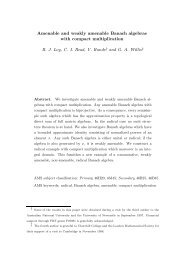
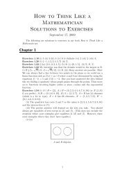
A STUDY OF TIME INTEGRATION SCHEMES FOR MODELLING FREE SURFACE FLOWSFigure 10. Drop advection problem.Drop Advection Problem3.73Drop Area3.72referenceTRBDFIMR0 50 100 150 200 250 300 350 400Time StepsFigure 11. Mass loss induced by time integration schemes.which is still popular in the computational science literature. It will not be included in ourstudy. The comparison that will be performed consists in measuring the mass (the area in2-D) of the drop for a given number of time steps. The numerical procedure for computingthe mass of the drop is explained in the Appendix.Figure 11 illustrates the performance of the TR, BDF and IMR schemes with respect tomass conservation. It may seem surprising that TR, which is one of the most popular timeintegration scheme used in CFD codes, performs poorly in our test. On the other hand, theIMR scheme which is not seen in many CFD papers, gives impressive results with respect tomass conservation. Quantitatively, we can observe, after only 400 non-dimensional time steps,for a xed time-step size of t =0:01 and for a mesh grid size x of the order of 0.07, amass loss of the order of 0.36% for TR while we have a mass loss of 0.001% for IMR.Copyright ? 2005 John Wiley & Sons, Ltd.Int. J. Numer. Meth. Fluids (in press)

A. MALIDI, S. DUFOUR AND D. N’DRIThis can be explained by the various properties of the IMR scheme [21]. This scheme issecond-order accurate, it introduces nearly no articial numerical oscillations, and it is A-stable, yet it introduces little undesirable damping compared to other A-stable schemes, whichmakes this scheme interesting for an advection equation. Constant-time-step size schemes areknown to give accurate results for a transport equation. Adaptive time integration schemesare suitable when the diusion term is non-negligible.6. OVERALL TIME INTEGRATION STRATEGY6.1. The time integration strategyBased on the results of the previous sections, the overall time integration strategy we proposefor modelling free surface ows using an Eulerian free surface capturing approach is composedof the ABDF scheme for the Navier–Stokes equations coupled with the IMR scheme for thetransport equation. Since we solve the system of partial dierential equations (2) and (3) ina coupled manner, the time steps used with the IMR scheme are the ones computed by theABDF scheme.This strategy allows us to combine the previously described properties of both schemes,and to avoid their drawbacks. The BDF scheme for the transport equation is too diusive,which would lead to the deformation of the pseudo-concentration and to mass loss. Moreover,an adaptive time integration scheme is not useful for an hyperbolic equation. In practice, weobserve that the time-step size reaches a constant value which corresponds to the chosentolerance, and it does not vary thereafter. The IMR scheme for the Navier–Stokes equationscould lead to numerical oscillations in the discretization of the velocity components.The proposed methodology is used to solve free surface ow problems of various nature inthe following subsections. First, we will model Taylor’s problem using the proposed methodology.This problem is known to reach a steady-state for specic operating conditions. TheABDF scheme should smoothly handle this problem. We will then study transient bubbleinteraction problems, which should be modelled accurately, with little mass loss, with thehelp of the IMR scheme.6.2. Numerical validation: Taylor’s problemLet us consider an initially undeformed ‘2-D circular drop’ of radius a = 1, located at thecentre of a computational domain of dimensions [−5; 5] × [−5; 5]. The mesh grid size for thissimulation is x =0:2. We are interested in the steady-state shape reached by the drop whensubmitted to a Cartesian linear ow. The far eld ow is described byu(x)= 1 ( )1+ 1 − x2 ˙ (17)−1+ −1 − )(ywhere ˙ is the shear rate of the ow and is a ow-type parameter. For example, the case = 1 corresponds to an extensional ow, while = 0 expresses a pure shear ow. The owsdescribed by Equation (17) are generated using the four-roll mill, developed by Taylor [24].The apparatus consists of four rotating cylinders, in the middle of which a drop is placed. ByCopyright ? 2005 John Wiley & Sons, Ltd.Int. J. Numer. Meth. Fluids (in press)

A STUDY OF TIME INTEGRATION SCHEMES FOR MODELLING FREE SURFACE FLOWSFigure 12. Steady-state shape of the drop and streamlines for Taylor’s problem.controlling the rotation rate of each cylinder, it is possible to obtain, far from the drop, thelinear velocity eld described by Equation (17).As an example, let us consider the case =0:2 with a viscosity ratio of = 1 = 2 =27:3(the drop is more viscous) and a density ratio of = 1 = 2 = 1. For a capillary number ofCa = 2˙a =0:082where the Navier–Stokes equations with the CSF model (5) are non-dimensionalized asReSt˜ @ũ@˜t + Re ˜(ũ · ˜∇)ũ = ˜∇ · ˜ + 1 Ca ˜ ˜∇Fit is observed experimentally [25] that the drop reaches a steady-state shape. Quantitiesdenoted with a tilde (‘˜’) represent non-dimensional values. The Reynolds number, Re, issmall in this application, which leads us to neglect the acceleration term. The ratio Re=St,which includes the Strouhal number St, is set to 1. Figure 12 illustrates the shape of thedrop and the streamlines, indicating that the steady-state seems to be reached. Figure 13 illustratesthe time-step sizes computed by the ABDF scheme, for a tolerance of =0:0005. Weagain observe larger time-step sizes for the transient phase of the simulation. The time-stepsizes become smaller when the drop reaches its steady-state shape and angle, where smalldeformations of the free surface are again captured by the transient error estimator.Copyright ? 2005 John Wiley & Sons, Ltd.Int. J. Numer. Meth. Fluids (in press)

A. MALIDI, S. DUFOUR AND D. N’DRI1.6Taylor’s Problem1.41.2Time-Step Sizes10.80.60.40.200 20 40 60 80 100 120 140 160Time StepsFigure 13. Time-step sizes for Taylor’s problem, using the ABDF scheme (Ca =0:082).Table I. Comparison of experimental and numericalresults for Taylor’s problem: =0:2, =27:3.Exper.Numer.Ca D D 0.082 0.0635 −28.0 0.1042 −28.00.164 0.0786 −34.0 0.1391 −34.00.246 0.0788 −35.0 0.1438 −35.00.329 0.0798 −35.0 0.1470 −35.0Taylor [24] dened a deformation parameter D asD = L − BL + Bwhere L and B are the longest and shortest semi-axes of the drop cross-section, in orderto measure the deformation of a drop. For various values of Ca, we computed thedeformation parameter D and the rotation angle of the drop. The results are comparedto the experimental data of Bentley and Leal [25] in Table I. It can be seen that the deformationparameter is nearly constant, this being the consequence of the rotational ow. Theconcave deformation curve, illustrated in Figure 14, is typical of this situation. Our overestimationof the deformation parameter is probably caused by the fact that we perform a2-D simulation of a 3-D problem. However, the computed angle of rotation reached by thenumerical drops is accurate.Copyright ? 2005 John Wiley & Sons, Ltd.Int. J. Numer. Meth. Fluids (in press)

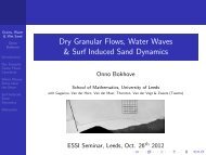
A STUDY OF TIME INTEGRATION SCHEMES FOR MODELLING FREE SURFACE FLOWS0.2experimental datanumerical resultsD00 0.6Figure 14. Deformation curve for Taylor’s problem: =0:2, =27:3.Ca6.3. Numerical validation: buoyancy-driven rising bubblesThe velocity and deformation of a single rising bubble due to buoyancy will rst be studied.This test is based on the results of Sussman and Smereka [26]. Let us consider a bubbleof non-dimensional radius ã = 1, which is initially lying at rest in another uid, in ageometry of dimensions [−3; 3] × [0; 12]. This system is submitted to a constant body forceg =(0; −g), where g is the gravitational acceleration. Since the uids have a density ratioof = 1 = 2 =0:0011 (the uid of the bubble is lighter), buoyancy generates a ow whichmakes the bubble rise. The viscosity ratio for this test is given by = 1 = 2 =0:0085.For this problem, the Navier–Stokes equations with the CSF model (5) arenon-dimensionalized as1St˜@ũ@˜t +˜(ũ · ˜∇)ũ = 1 Re ˜∇ · ˜ + 1 Fr ˜ ˜g + 1 We ˜ ˜∇F (18)where, in our case, the Reynolds number is given bythe Froude number is dened asRe = au 0 2 2=9:8Fr = u2 0ag =0:76Copyright ? 2005 John Wiley & Sons, Ltd.Int. J. Numer. Meth. Fluids (in press)

A. MALIDI, S. DUFOUR AND D. N’DRI(a) t = 0.0 (b) t = 3.6 (c) t = 4.8 (d) t = 6.0Figure 15. Buoyancy-driven rising of a single bubble.and the Weber number is given byWe = a2 g 2=7:6where the reference velocity u 0 is the experimentally observed [27] steady-state rise velocityof an air bubble, which is u 0 =21:5cm=s. The Strouhal number St is again set to 1. The otherquantities were previously described.Figure 15 illustrates the deformation of the rising bubble at various time steps. The simulationwas performed for the complete bubble. Our methodology performs well in maintainingthe symmetry of the bubble, and its vertical path. Since this simulation is performed usinga Cartesian frame of reference, the computed shapes of the bubble dier slightly from theones illustrated in Reference [26]. The computed rising speed of the bubble is underestimatedwhen compared to the non-dimensional rising speed which should be equal to 1, this beingcaused again by our 2-D approximation of an axisymmetric phenomena. Finally, usingour methodology, we measure a numerical mass loss of the order of 8% over 80 time steps(t =0;:::;6:5).We will now study the rise and interaction of two bubbles due to buoyancy. It is a commonpractice in the literature to describe bubbles dynamics problems using the Eotvos number,also known as the Bond numberEo = 2gL 2 0and the Archimedes number, also known as the Galileo numberN = 2 2 gL3 0 2 2Copyright ? 2005 John Wiley & Sons, Ltd.Int. J. Numer. Meth. Fluids (in press)

A STUDY OF TIME INTEGRATION SCHEMES FOR MODELLING FREE SURFACE FLOWSFigure 16. Bubbles rising problem.(a) t = 0.00 (b) t = 2.39 (c) t = 2.99 (c) t = 3.43Figure 17. Buoyancy-driven rising and coalescence of two bubbles.The Morton number is also seen in the literature:M = g4 2 2 = Eo33 N 2However, it is possible to still work with the non-dimensionalized equations (18) by deningthe reference velocity as u 0 = √ gL 0 , which gives us a relation between the non-dimensionalgroups (Re; Fr; We) and (N; Eo). In our case, Re = √ N, Fr = 1 and We = Eo.Our test problem, described in Reference [28], is illustrated in Figure 16. It consists of twovertically aligned bubbles with same diameter d =2:6 mm, located at a distance of h =0:4mmCopyright ? 2005 John Wiley & Sons, Ltd.Int. J. Numer. Meth. Fluids (in press)

A. MALIDI, S. DUFOUR AND D. N’DRI2Rising Drops ProblemreferencedropsTotal Area of the Drops100 2 4TimeFigure 18. Rising and coalescence of two bubbles: mass conservation.from each other. The non-dimensional groups are given by Re = √ N = 30 and Eo = We = 100.Finally, the density ratio is given by = 2 = 1 = 2 and the viscosity ratio is = 2 = 1 =2.Figure 17 illustrates the deformation and coalescence of the two rising bubbles at varioustime steps. The shape of the drops are similar to what we can observe in Reference [28], thedierence coming from the fact that these results come from 3-D simulations. We observethat coalescence occurs after 29 time steps (˜t =3:43). Figure 18 illustrates the variation of thetotal mass of the bubbles (non-dimensional area) for the duration of the simulation, which isvery small. It is unfortunately dicult to nd quantitative results in the literature in order toperform an accurate validation for this problem.7. CONCLUSIONA time integration strategy is proposed for modelling free surface ows in the context ofEulerian interface capturing. An adaptive second-order accurate backward dierentiation formulais used to discretize the transient term of the Navier–Stokes equations, and the implicitmidpoint rule is used for the transport equation of the marker variable. The adaptive schemeallows the automatic determination of a time-step size that follows the physics of the problemunder study. It is shown that this mixed strategy gives accurate results for steady-state freesurface ows, and that it reduces mass loss for transient multiuid ows. Such a study isnovel to our knowledge. It also seems that it is the rst time that the ABDF scheme wasused in an applied context.In order to keep the focus of this study on time integration strategies, several componentsof the numerical model necessary for performing accurate free surface ow simulations wereCopyright ? 2005 John Wiley & Sons, Ltd.Int. J. Numer. Meth. Fluids (in press)

A STUDY OF TIME INTEGRATION SCHEMES FOR MODELLING FREE SURFACE FLOWSnot discussed in this paper. Maintaining the region of transition of the pseudo-concentrationsharp but smooth is very important in order to perform the accurate modelling of surfacetension. Mesh adaptation in the vicinity of the free surface is also important for accuratelymodelling interfacial physics. The accurate numerical modelling of the capillary force is alsoa delicate matter. These questions were studied in References [5, 6, 16, 20] and we are stillmaking progress developing more accurate algorithms for addressing these questions. Futurework also includes the development of an axisymmetric model which should allow us toobtain numerical results that are closer to what is observed experimentally. We also plan tostudy applied (industrial) free surface ows involving the dynamics of drops and bubbles suchas emulsions and jet break-ups.APPENDIX A: COMPUTING THE AMOUNT OF MASS FOR EACH FLUIDVerifying mass conservation for each uid is not a straightforward process in the contextof Eulerian free surface capturing. The fact that we are working with non-structured meshesmakes it more dicult to nd an algorithm for computing the area of the regions 1 and 2 .When the interface does not go through an element, i.e. there are no points x in the elementsuch that F(x)= 1 2, the area of the triangle gives the quantity of mass of uid 1 or 2 in thatelement. The other possibility is to see the interface S go through an element, as illustrated inFigure A1. A rst approximation will be obtained by locating the two points of intersectionof the free surface with the sides of the element (the points 2 and 5 in Figure A2(a)). Thequantity of uid 1 is approximated by the area of the triangle with vertices 1; 2 and 5, andthe quantity of uid 2 by the area of the quadrangle with vertices 2; 3; 4 and 5. We canthen repeat this process by subdividing the element, as illustrated in Figure A2(b), and bycomputing the area occupied by each uid in the subtriangles, as described above. We thenrepeat this subdivision process (cf. Figure A2(c)) until convergence of the computed area ofthe regions occupied by each uid in that element, for a given tolerance. We observe that wecompute the mass for each uid to machine precision after 3 or 4 levels of subdivisions.Figure A1. Elementary free surface ow problem.Copyright ? 2005 John Wiley & Sons, Ltd.Int. J. Numer. Meth. Fluids (in press)

A. MALIDI, S. DUFOUR AND D. N’DRI(a) (b) (c)Figure A2. Mass computation for each uid: (a) rst level; (b) second level; and (c) third level.ACKNOWLEDGEMENTSThis work was sponsored in part by the Auto21 Network of Centres of Excellence of Canada, theNatural Sciences and Engineering Research Council of Canada and the Fonds quebecois de la recherchesur la nature et les technologies.REFERENCES1. Floryan JM, Rasmussen H. Numerical methods for viscous ows with moving boundaries. In Applied MechanicsReview, Metzner AWK (ed.). ASME: New York, 1989; 323–341.2. Hirt CW, Nichols BD. Volume of uid (VOF) method for the dynamics of free boundaries. Journal ofComputational Physics 1981; 39:201–225.3. Sethian JA. Level Set Methods. Evolving Interfaces in Geometry, Fluid Mechanics, Computer Vision, andMaterials Science. Cambridge University Press: Cambridge, MA, 1999.4. Thompson E. Use of pseudo-concentration to follow creeping viscous ows during transient analysis.International Journal for Numerical Methods in Fluids 1986; 6:749–761.5. Dufour S, Malidi A. A free surface updating methodology for marker function-based Eulerian free surfacecapturing techniques on unstructured meshes. Communications in Numerical Methods in Engineering 2004;20:857–867.6. Dufour S, Pelletier D. Computations of multiphase ows with surface tension using an adaptive nite elementmethod. Numerical Heat Transfer, Part A 2001; 40:335–362.7. Johnson C. Numerical Solution of Partial Dierential Equations by the Finite Element Method. CambridgeUniversity Press: Cambridge, MA, 1987.8. Gao DM. A three-dimensional hybrid nite element-volume tracking model for mould lling in casting processes.International Journal for Numerical Methods in Fluids 1999; 29:877–895.9. Tezduyar ET, Aliabadi S. EDICT for 3D computation of two-uid interfaces. Computer Methods in AppliedMechanics and Engineering 2000; 190:403–410.10. Beliveau A, Fortin A, Demay Y. A two-dimensional numerical method for the deformation of drops with surfacetension. International Journal of Computational Fluid Dynamics 1998; 10:225–240.11. Fortin M, Fortin A. A generalization of Uzawa’s algorithm for the solution of the Navier–Stokes equations.Communications in Applied Numerical Methods 1985; 1:205–208.12. Brackbill JU, Kothe DB, Zemach C. A continuum method for modeling surface tension. Journal ofComputational Physics 1992; 100:335–354.13. Rudman M. A volume-tracking method for incompressible multiuid ows with large density variations.International Journal for Numerical Methods in Fluids 1998; 28:357–378.14. Williams MW, Kothe DB, Puckett EG. Accuracy and convergence of continuum surface-tension models. InFluid Dynamics at Interfaces, Shyy W, Narayanan R (eds). Cambridge University Press: Cambridge, MA,1999; 294–305.15. Popinet S, Zaleski S. A front-tracking algorithm for accurate representation of surface tension. InternationalJournal for Numerical Methods in Fluids 1999; 30:775–793.16. Dufour S, Pelletier D. A study of drop dynamics using an adaptive nite element method. 14th AIAAComputational Fluid Dynamics Conference, Norfolk, VA, AIAA Paper 99-3318, 1999; 12.Copyright ? 2005 John Wiley & Sons, Ltd.Int. J. Numer. Meth. Fluids (in press)

A STUDY OF TIME INTEGRATION SCHEMES FOR MODELLING FREE SURFACE FLOWS17. Renardy Y, Renardy M. PROST: a parabolic reconstruction of surface tension for the volume-of-uid method.Journal of Computational Physics 2002; 183:400–421.18. Shin S, Abdel-Khalik SI, Daru V, Juric D. Accurate representation of surface tension using the level contourreconstruction method. Journal of Computational Physics 2005; 203:493–516.19. Hou TY, Lowengrub JS, Shelley MJ. Removing the stiness from interfacial ows with surface tension. Journalof Computational Physics 1994; 114:312–338.20. Dufour S, Malidi A. An Eulerian interface capturing methodology for the numerical modeling of free surfaceows with surface tension. Redaction, 2005.21. Gresho PM, Sani RL, Engelman MS. Incompressible Flow and the Finite Element Method: Advection–Diusionand Isothermal Laminar Flow. Wiley: New York, 1999.22. Cuvelier C, Segal A, van Steenhoven AA. Finite Element Methods and Navier–Stokes Equations. D. ReidelPublishing Company: Dordrecht, 1986.23. Engelman SE, Jamnia M-A. Transient ow past a circular cylinder: a benchmark solution. International Journalfor Numerical Methods in Fluids 1990; 11:985–1000.24. Taylor GI. The formation of emulsions in denable elds of ow. Proceedings of the Royal Society of London1934; 146(A):501–523.25. Bentley BJ, Leal LG. An experimental investigation of drop deformation and breakup in steady, two-dimensionallinear ows. Journal of Fluid Mechanics 1986; 167:241–283.26. Sussman M, Smereka P. Axisymmetric free boundary problems. Journal of Fluid Mechanics 1997; 341:269–294.27. Hnat JG, Buckmaster JD. Spherical cap bubbles and skirt formation. Physics of Fluids 1976; 19:182–194.28. de Sousa FS, Mangiavacchi N, Nonato LG, Castelo A, Tome MF, Ferreira VG, Cuminato JA, McKee S. Afront-tracking=front-capturing method for the simulation of 3D multi-uid ows with free surfaces. Journal ofComputational Physics 2004; 198:469–499.Copyright ? 2005 John Wiley & Sons, Ltd.Int. J. Numer. Meth. Fluids (in press)