A study of time integration schemes for the numerical modelling of ...

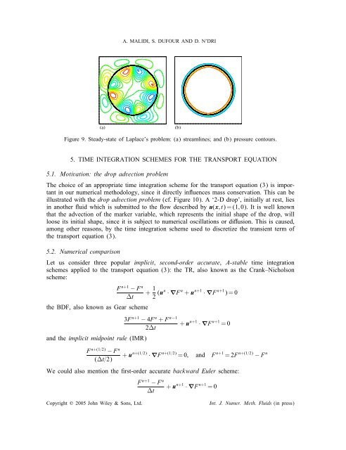
A. MALIDI, S. DUFOUR AND D. N’DRI(a)(b)Figure 9. Steady-state of Laplace’s problem: (a) streamlines; and (b) pressure contours.5. TIME INTEGRATION SCHEMES FOR THE TRANSPORT EQUATION5.1. Motivation: the drop advection problemThe choice of an appropriate time integration scheme for the transport equation (3) is importantin our numerical methodology, since it directly inuences mass conservation. This can beillustrated with the drop advection problem (cf. Figure 10). A ‘2-D drop’, initially at rest, liesin another uid which is submitted to the ow described by u(x;t)=(1; 0). It is well knownthat the advection of the marker variable, which represents the initial shape of the drop, willloose its initial shape, since it is subject to numerical oscillations or diusion. This is caused,among other reasons, by the time integration scheme used to discretize the transient term ofthe transport equation (3).5.2. Numerical comparisonLet us consider three popular implicit, second-order accurate, A-stable time integrationschemes applied to the transport equation (3): the TR, also known as the Crank–Nicholsonscheme:F n+1 − F n+ 1 t 2 (un · ∇F n + u n+1 · ∇F n+1 )=0the BDF, also known as Gear scheme3F n+1 − 4F n + F n−1+ u n+1 · ∇F n+1 =02tand the implicit midpoint rule (IMR)F n+(1=2) − F n(t=2)+ u n+(1=2) · ∇F n+(1=2) =0; and F n+1 =2F n+(1=2) − F nWe could also mention the rst-order accurate backward Euler scheme:F n+1 − F n+ u n+1 · ∇F n+1 =0tCopyright ? 2005 John Wiley & Sons, Ltd.Int. J. Numer. Meth. Fluids (in press)