OCS Study MMS 95 - Data Center

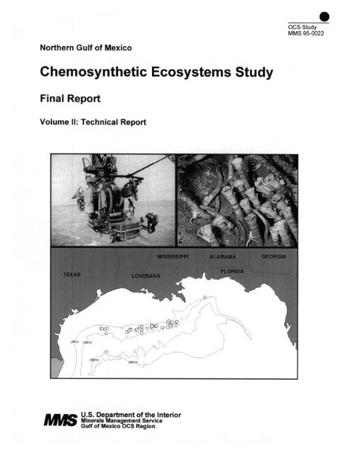
OCS StudyMMS 95-0022Northern Gulf of MexicoChemosynthetic Ecosystems StudyFinal ReportVolume II :Technical ReportMISSISSIPPI ALABAMA GEORGIATEXASFLORIDALOUISIANA =- .~ .. ,'U.S . Department of the InteriorMinerals Management ServiceGulf of Mexico OCS Region

OCS StudyMMS 95-0022Northern Gulf of MexicoChemosynthetic Ecosystems StudyFinal ReportVolume II :Technical ReportEditorsIan R . MacDonaldWilliam W. SchroederandJames M . BrooksPrepared under MMS Contract14-35-0001-30555byGeochemical and Environmental Research GroupTexas A&M UniversityTexas A&M Research FoundationCollege Station, TexasPublished byU .S . Department of the InteriorMinerals Management ServiceNew OrleansGulf of Mexico OCS Region May 1996

DISCLAIMER.This report was prepared under contract between the Minerals Management Service(MMS) and Geochemical and Environmental Research Group . This report has beentechnically reviewed by the MMS and approved for publication . Approval does notsignify that the contents necessarily reflect the views and policies of the Service, nordoes mention of trade names or commercial products constitute endorsement orrecommendation for use . It is, however, exempt from review and compliance withMMS editorial standards .REPORT AVAILABILITYExtra copies of the report may be obtained from the Public Information Unit (MailStop 5034) at the following address :U.S . Department of the InteriorMinerals Management ServiceGulf of Mexico OCS RegionPublic Information Unit (MS 5034)1201 Elmwood Park BoulevardNew Orleans, Louisiana 70123-2394Telephone Number : (504) 736-25191-800-200-GULFSuggested citation :CITATIONMacDonald, I .R ., W.W . Schroeder, and J.M . Brooks . 1995 . ChemosyntheticEcosystems Studies Final Report . Prepared by Geochemical andEnvironmental Research Group . U.S . Dept . of the Interior, Minerals Mgmt .Service, Gulf of Mexico OCS Region, New Orleans, LA . OCS Study MMS 95-0023 . 338 pp .COVER PHOTOGRAPHThe foreground photograph shows the submersible Johnson Sea-Link I preparing forone of its many dives to study chemosynthetic ecosystems . The map depicts thelocations of known chemosynthetic ecosystems in the northern Gulf of Mexico .iii

PREFACEThe Chemosynthetic Ecosystems Study concerns the prominent biologicalcommunities of tube worms, mussels, and clams that occur at natural hydrocarbonseeps on the continental slope and that derive their food supply from chemicalsassociated with the seeps .This is the Technical Report (Volume II) of the FinalReport that will be issued by the Study, which is sponsored by the U.S .Departmentof Interior Minerals Management Service (MMS), Gulf of Mexico Region OCS Office(Contract 14-35-0001-30555) .The Study is being conducted by ten principal investigators (PIs) and fourassociates under the overall management of the Geochemical and EnvironmentalResearch Group (GERG) of Texas A&M University (see next page) .The Programhas completed all of the three scheduled research cruises and has completedprocessing material collected on these cruises .The first report of the Study(MacDonald 1992) presented a review of published literature pertinent to the subjectand a limited synthesis of data collected prior to commencement of the Program.Anappendix volume to this report reproduced the core, peer-reviewed literature pertinentto Gulf of Mexico seep communities An interim report described the methods,techniques, and equipment used during the field program, outlined the data sets andcollections obtained during the field study, and discussed the analyses andinterpretations employed to treat these materials .This report comprises some of theintroductory material from the two previous reports in order to provide unfamiliarreaders with a context for Study findings .In keeping with MMS guidelines, thesechapters are addressed to an audience of knowledgeable lay-people .To enhancereadability, extended listings of materials and methods will be given in an appendixvolume or by citation to previous reports or publications .v

Principal Investigators (*) and Associates for the Chemosynthetic EcosystemsStudy . Affiliation abbreviations are :TAMU Texas A&M UniversityGERG Geoctcemical and Environmental Research Group ;TAMUOCNG Oceanography Department, Texas A&M UniversityLSU Louisiana State UniversityPSU Pennsylvania State UniversityWHOI Woods Hole Oceanographic InstitutionUA/DISL University of Alabama, Dauphin Island Sea LabPrincipal Investigator Affiliation Major ResponsibilityJavier Alcala-Herrera TAMU/GERG Chemical AnalysesJames M . Brooks* TAMU/GERG Project DirectorRobert S . Carney* LSU EcologyCharles R. Fisher* PSU PhysiologyNorman L . Guinasso, Jr.* TAMU/GERG Data AnalysisHolgar W. Jannasch* WHOI MicrobiologyMahlon C . Kennicutt II* TAMU/GERG GeochemistryIan R. MacDonald* TAMU/GERG Ecology/Deputy Project DirectorEric N . Powell* TAMU/OCNG TaphonomyWilliam S . Sager* TAMU/OCNG GeologyWilliam W. Schroeder* UA/DISL Geology/EcologyDan L . Wilkinson TAMU/GERG Field LogisticsCarl O . Wirsen WHOI MicrobiologyGary A Wolff TAMU/GERG Data Managementvii

TABLE OF CONTENTSPageList of Figures . . . . . . . . . . . . . . . . . . . . . . . . . . . . . . . . . . . . . . . . . . . . . . . . . . . . . . . . . . . . . . . . . . . . . . . . . . . . . . . . . . . . . . . . . . . . . . . . . . . . . . . . . . . . . . . . . . . . . . . . . . . . xvList of Tables . . . . . . . . . . . . . . . . . . . . . . . . . . . . . . . . . . . . . . . . . . . . . . . . . . . . . . . . . . . . . . . . . . . . . . . . . . . . . . . . . . . . . . . . . . . . . . . . . . . . . . . . . . . . . . . . . . . . . . . . . . . . . .)cd1 .0 Chemosynthetic Ecosystems Study: Overview . . . . . . . . . . . . . . . . . . . . . . . . . . . . . . . . . . . . . . . . . . . . 1-11 .1 Chemosynthetic Communities in the Gulf of Mexico . . . . . . . . . . . . . . . . . . . . . . . . . . . . . . . . l-11 .2 Summary of Study Accomplishments . . . . . . . . . . . . . . . . . . . . . . . . . . . . . . . . . . . . . . . . . . . . . . . . . . . . . . . . . l-32.0 The Regional Distribution of Chemosynthetic CommunitiesAcross the Continental Slope in the Northern Gulf of Mexico . . . . . . . . . . . . . . . . 2-12.1 Introduction . . . . . . . . . . . . . . . . . . . . . . . . . . . . . . . . . . . . . . . . . . . . . . . . . . . . . . . . . . . . . . . . . . . . . . . . . . . . . . . . . . . . . . . . . . . . . . . . . . . . ..2-12.2 Types of Seep Communities . . . . . . . . . . . . . . . . . . . . . . . . . . . . . . . . . . . . . . . . . . . . . . . . . . . . . . . . . . . . . . . . . . . . . . . ..2-22.3 Zonal Distribution of Chemosynthetic Communities in theNorthern Gulf of Mexico . . . . . . . . . . . . . . . . . . . . . . . . . . . . . . . . . . . . . . . . . . . . . . . . . . . . . . . . . . . . . . . . . . . . . . . . . . . . . . . . . .2-32 .3 .1 Local Patterns . . . . . . . . . . . . . . . . . . . . . . . . . . . . . . . . . . . . . . . . . . . . . . . . . . . . . . . . . . . . . . . . . . . . . . . . . . . . . . . . . . . ..2-32 .3 .2 Regional Patterns . . . . . . . . . . . . . . . . . . . . . . . . . . . . . . . . . . . . . . . . . . . . . . . . . . . . . . . . . . . . . . . . . . . . . . . . . . . . . . ..2-62.4 Remote-Sensing Detection of Natural Oil Seepage . . . . . . . . . . . . . . . . . . . . . . . . . . . . . . . . . . . 2-82 .4.1 Use of Geophysical Methods for Indirect Detection ofChemosynthetic Communities . . . . . . . . . . . . . . . . . . . . . . . . . . . . . . . . . . . . . . . . . . . . . . . . . . . . . . . . . .2-82 .4.2 Formation and Detection of Surface Oil Slicks . . . . . . . . . . . . . . . . . . . . . . . . . . . . . .2-92 .4.3 Remote Sensing Methods . . . . . . . . . . . . . . . . . . . . . . . . . . . . . . . . . . . . . . . . . . . . . . . . . . . . . . . . . . . . . . . . 2-102 .4.4 Estimates of Total Seepage . . . . . . . . . . . . . . . . . . . . . . . . . . . . . . . . . . . . . . . . . . . . . . . . . . . . . . . . . . . . 2-162 .4.5 Trial of the Laser Line Scan System . . . . . . . . . . . . . . . . . . . . . . . . . . . . . . . . . . . . . . . . . . . . 2-202.5 Summary . . . . . . . . . . . . . . . . . . . . . . . . . . . . . . . . . . . . . . . . . . . . . . . . . . . . . . . . . . . . . . . . . . . . . . . . . . . . . . . . . . . . . . . . . . . . . . . . . . . . . . . .2-213.0 Geological and Geophysical Characterization of Hydrocarbons . . . . . . . . . . .3-13 .1 Introduction . . . . . . . . . . . . . . . . . . . . . . . . . . . . . . . . . . . . . . . . . . . . . . . . . . . . . . . . . . . . . . . . . . . . . . . . . . . . . . . . . . . . . . . . . . . . . . . . . . . . . ..3-13.1.1 Study Locations . . . . . . . . . . . . . . . . . . . . . . . . . . . . . . . . . . . . . . . . . . . . . . . . . . . . . . . . . . . . . . . . . . . . . . . . . . . . . . . . . . . .3-23.1.2 Geologic Causes and Symptoms of Hydrocarbon Seeps inthe Gulf of Mexico . . . . . . . . . . . . . . . . . . . . . . . . . . . . . . . . . . . . . . . . . . . . . . . . . . . . . . . . . . . . . . . . . . . . . . . . . . . . . . . . .3-23.1 .3 Geophysical Signatures of Seeps . . . . . . . . . . . . . . . . . . . . . . . . . . . . . . . . . . . . . . . . . . . . . . . . . . . . ..3-53 .2 Data . . . . . . . . . . . . . . . . . . . . . . . . . . . . . . . . . . . . . . . . . . . . . . . . . . . . . . . . . . . . . . . . . . . . . . . . . . . . . . . . . . . . . . . . . . . . . . . . . . . . . . . . . . . . . . . . . . ..3-73.3 Objectives . . . . . . . . . . . . . . . . . . . . . . . . . . . . . . . . . . . . . . . . . . . . . . . . . . . . . . . . . . . . . . . . . . . . . . . . . . . . . . . . . . . . . . . . . . . . . . . . . . . . . . . 3-103.4 Methods . . . . . . . . . . . . . . . . . . . . . . . . . . . . . . . . . . . . . . . . . . . . . . . . . . . . . . . . . . . . . . . . . . . . . . . . . . . . . . . . . . . . . . . . . . . . . . . . . . . . . . . . . . . 3-103.5 Results . . . . . . . . . . . . . . . . . . . . . . . . . . . . . . . . . . . . . . . . . . . . . . . . . . . . . . . . . . . . . . . . . . . . . . . . . . . . . . . . . . . . . . . . . . . . . . . . . . . . . . . . . . . . . 3-14

3 .5 .1 Acoustic Echo Types . . . . . . . . . . . . . . . . . . . . . . . . . . . . . . . . . . . . . . . . . . . . . . . . . . . . . . . . . . . . . . . . . . . . . . ..3-143 .5 .2 Ground Truth . . . . . . . . . . . . . . . . . . . . . . . . . . . . . . . . . . . . . . . . . . . . . . . . . . . . . . . . . . . . . . . . . . . . . . . . . . . . . . . . . . . . . . 3-163 .5 .3 Distribution of Echo Types . . . . . . . . . . . . . . . . . . . . . . . . . . . . . . . . . . . . . . . . . . . . . . . . . . . . . . . . . . . . . . 3-193 .5 .4 Backscatter Mosaics . . . . . . . . . . . . . . . . . . . . . . . . . . . . . . . . . . . . . . . . . . . . . . . . . . . . . . . . . . . . . . . . . . . . . . . . 3-253 .5 .5 Connections to Deep Faults . . . . . . . . . . . . . . . . . . . . . . . . . . . . . . . . . . . . . . . . . . . . . . . . . . . . . . . . . . . . 3-313 .5 .6 Relationship of Geophysical Signatures and SeepOrganisms . . . . . . . . . . . . . . . . . . . . . . . . . . . . . . . . . . . . . . . . . . . . . . . . . . . . . . . . . . . . . . . . . . . . . . . . . . . . . . . . . . . . . . . . . . . 3-313 .6 Discussion . . . . . . . . . . . . . . . . . . . . . . . . . . . . . . . . . . . . . . . . . . . . . . . . . . . . . . . . . . . . . . . . . . . . . . . . . . . . . . . . . . . . . . . . . . . . . . . . . . . . . . .3-344.0 Geochemical Alteration of Hydrocarbons in Seep Systems . . . . . . . . . . . . . . . . . . ..4-14.1 Introduction : A Descriptive Model of the Geochemical Setting ofSeep Communities . . . . . . . . . . . . . . . . . . . . . . . . . . . . . . . . . . . . . . . . . . . . . . . . . . . . . . . . . . . . . . . . . . . . . . . . . . . . . . . . . . . . . . . . . ..4-14.2 Experimental . . . . . . . . . . . . . . . . . . . . . . . . . . . . . . . . . . . . . . . . . . . . . . . . . . . . . . . . . . . . . . . . . . . . . . . . . . . . . . . . . . . . . . . . . . . . . . . . . . 4-134.2 .1 Samples . . . . . . . . . . . . . . . . . . . . . . . . . . . . . . . . . . . . . . . . . . . . . . . . . . . . . . . . . . . . . . . . . . . . . . . . . . . . . . . . . . . . . . . . . . . . . . . 4-134 .2 .2 Methods . . . . . . . . . . . . . . . . . . . . . . . . . . . . . . . . . . . . . . . . . . . . . . . . . . . . . . . . . . . . . . . . . . . . . . . . . . . . . . . . . . . . . . . . . . . . . ..4-154.3 R.esults . . . . . . . . . . . . . . . . . . . . . . . . . . . . . . . . . . . . . . . . . . . . . . . . . . . . . . . . . . . . . . . . . . . . . . . . . . . . . . . . . . . . . . . . . . . . . . . . . . . . . . . . . . . . . 4-164.3 .1 Isolated Bacterial Mat at GC 234 . . . . . . . . . . . . . . . . . . . . . . . . . . . . . . . . . . . . . . . . . . . . . . . . . 4-164.3 .2 Bacterial Mat and Tube Worms at GC 185 (Bush Hill) . . . . . . . . . . . . 4-204 .3 .3 Gas Hydrate at GC 185 (Bush Hill) . . . . . . . . . . . . . . . . . . . . . . . . . . . . . . . . . . . . . . . . . . . . . . 4-204 .3 .4 Chemosynthetic Clams at GC 272 . . . . . . . . . . . . . . . . . . . . . . . . . . . . . . . . . . . . . . . . . . . . . . . 4-204.3.5 Chemosynthetic Mussels at GC 233 . . . . . . . . . . . . . . . . . . . . . . . . . . . . . . . . . . . . . . . . . . . . 4-214.4 Discussion . . . . . . . . . . . . . . . . . . . . . . . . . . . . . . . . . . . . . . . . . . . . . . . . . . . . . . . . . . . . . . . . . . . . . . . . . . . . . . . . . . . . . . . . . . . . . . . . . . . . . . . 4-214.4 .1 Hydrocarbons . . . . . . . . . . . . . . . . . . . . . . . . . . . . . . . . . . . . . . . . . . . . . . . . . . . . . . . . . . . . . . . . . . . . . . . . . . . . . . . . . . . ..4-214.4 .2 Seeps and Vents . . . . . . . . . . . . . . . . . . . . . . . . . . . . . . . . . . . . . . . . . . . . . . . . . . . . . . . . . . . . . . . . . . . . . . . . . . . . . . . . 4-294.4 .3 Sea-floor Modification at Seeps . . . . . . . . . . . . . . . . . . . . . . . . . . . . . . . . . . . . . . . . . . . . . . . . . . . . . . 4-304.5 Conclusions . . . . . . . . . . . . . . . . . . . . . . . . . . . . . . . . . . . . . . . . . . . . . . . . . . . . . . . . . . . . . . . . . . . . . . . . . . . . . . . . . . . . . . . . . . . . . . . . . . . ..4-345.0 Characterization of Habitats and Determination of Growth Rateand Approximate Ages of the Chemosynthetic Symbiont-Containing Fauna . . . . . . . . . . . . . . . . . . . . . . . . . . . . . . . . . . . . . . . . . . . . . . . . . . . . . . . . . . . . . . . . . . . . . . . . . . . . . . . . . . . . . . . . . . . . . . . . . . . ..5-15.1 Mussel Methods . . . . . . . . . . . . . . . . . . . . . . . . . . . . . . . . . . . . . . . . . . . . . . . . . . . . . . . . . . . . . . . . . . . . . . . . . . . . . . . . . . . . . . . . . . . . . . ..5-25.2 Water Sampling and Analysis . . . . . . . . . . . . . . . . . . . . . . . . . . . . . . . . . . . . . . . . . . . . . . . . . . . . . . . . . . . . . . . . . . . . . . .5-35 .3 Growth Studies . . . . . . . . . . . . . . . . . . . . . . . . . . . . . . . . . . . . . . . . . . . . . . . . . . . . . . . . . . . . . . . . . . . . . . . . . . . . . . . . . . . . . . . . . . . . . . . ..5-55 .4 Transplant Experiment . . . . . . . . . . . . . . . . . . . . . . . . . . . . . . . . . . . . . . . . . . . . . . . . . . . . . . . . . . . . . . . . . . . . . . . . . . . . . . . . . .5-65.4.1 Measures of Condition . . . . . . . . . . . . . . . . . . . . . . . . . . . . . . . . . . . . . . . . . . . . . . . . . . . . . . . . . . . . . . . . . . . . . . . . .5-65 .5 Statistical Methods . . . . . . . . . . . . . . . . . . . . . . . . . . . . . . . . . . . . . . . . . . . . . . . . . . . . . . . . . . . . . . . . . . . . . . . . . . . . . . . . . . . . . . . . ..5-85 .6 Growth Methods . . . . . . . . . . . . . . . . . . . . . . . . . . . . . . . . . . . . . . . . . . . . . . . . . . . . . . . . . . . . . . . . . . . . . . . . . . . . . . . . . . . . . . . . . . . . . ..5-9X

5.7 Results for Vestimentiferans : Escarpicz sp . and Lamellibrachiasp . . . . . . . . . . . . . . . . . . . . . . . . . . . . . . . . . . . . . . . . . . . . . . . . . . . . . . . . . . . . . . . . . . . . . . . . . . . . . . . . . . . . . . . . . . . . . . . . . . . . . . . . . . . . . . . . . . . . . . . . .5-95 .7 .1 Vestimentiferan Growth Rates . . . . . . . . . . . . . . . . . . . . . . . . . . . . . . . . . . . . . . . . . . . . . . . . . . . . . . 5-105 .7 .2 Vestimentiferan Habitat Characterization . . . . . . . . . . . . . . . . . . . . . . . . . . . . . . . . . 5-155 .7 .3 Vestimentiferan Condition at Different Sites . . . . . . . . . . . . . . . . . . . . . . . . . . . . . . 5-185 .8 Results for Vesicomyid Clams : Vesicomya chordates andCczlyptogena ponderasa . . . . . . . . . . . . . . . . . . . . . . . . . . . . . . . . . . . . . . . . . . . . . . . . . . . . . . . . . . . . . . . . . . . . . . . . . . . . . . . . . 5-215 .9 Results for the Methane Mussel : Seep Mytilid Ia (SM Ia) . . . . . . . . . . . . . . . . . . . . 5-245.9.1 The Mussel Beds . . . . . . . . . . . . . . . . . . . . . . . . . . . . . . . . . . . . . . . . . . . . . . . . . . . . . . . . . . . . . . . . . . . . . . . . . . . . . . . . 5-255.9 .1 .1 GC 184 Mussel Beds . . . . . . . . . . . . . . . . . . . . . . . . . . . . . . . . . . . . . . . . . . . . . . . . . . . . . . . . . . 5-255.9 .1 .2 GC 234 Mussel Beds . . . . . . . . . . . . . . . . . . . . . . . . . . . . . . . . . . . . . . . . . . . . . . . . . . . . . . . . . . 5-295 .9 .1 .3 GC 272 Mussel Bed . . . . . . . . . . . . . . . . . . . . . . . . . . . . . . . . . . . . . . . . . . . . . . . . . . . . . . . . . . . . 5-295.9 .2 SM Ia Population Structure . . . . . . . . . . . . . . . . . . . . . . . . . . . . . . . . . . . . . . . . . . . . . . . . . . . . . . . . . . . . 5-305.9 .3 SM Ia Chemical Microhabitat . . . . . . . . . . . . . . . . . . . . . . . . . . . . . . . . . . . . . . . . . . . . . . . . . . . . . . . . 5-305.9 .4 Growth Rates and Ages of SM Ia . . . . . . . . . . . . . . . . . . . . . . . . . . . . . . . . . . . . . . . . . . . . . . . . . . . 5-365.9 .5 Measures of Condition of SM Ia . . . . . . . . . . . . . . . . . . . . . . . . . . . . . . . . . . . . . . . . . . . . . . . . . . . . . 5-415.9 .6 Transplant Studies with SM Ia . . . . . . . . . . . . . . . . . . . . . . . . . . . . . . . . . . . . . . . . . . . . . . . . . . . . . . 5-425.9 .7 Site Synopsis for SM Ia Beds . . . . . . . . . . . . . . . . . . . . . . . . . . . . . . . . . . . . . . . . . . . . . . . . . . . . . . . . . 5-445.10 Implications of Growth Experiments and HabitatCharacterizations on MMS Management Concerns . . . . . . . . . . . . . . . . . . . . . . . . . . . . . 5-466.0 Sessile Macrofauna and Megafauna at Mussel Beds . . . . . . . . . . . . . . . . . . . . . . . . . . . . . . . . . .6-16.1 Introduction . . . . . . . . . . . . . . . . . . . . . . . . . . . . . . . . . . . . . . . . . . . . . . . . . . . . . . . . . . . . . . . . . . . . . . . . . . . . . . . . . . . . . . . . . . . . . . . . . . . . . ..6-16.2 Methods and Design . . . . . . . . . . . . . . . . . . . . . . . . . . . . . . . . . . . . . . . . . . . . . . . . . . . . . . . . . . . . . . . . . . . . . . . . . . . . . . . . . . . . . . . . .6-26.2.1 Sampling Methods . . . . . . . . . . . . . . . . . . . . . . . . . . . . . . . . . . . . . . . . . . . . . . . . . . . . . . . . . . . . . . . . . . . . . . . . . . . . . . ..6-26.2.2 Sampling Design . . . . . . . . . . . . . . . . . . . . . . . . . . . . . . . . . . . . . . . . . . . . . . . . . . . . . . . . . . . . . . . . . . . . . . . . . . . . . . . . . ..6-36.3 Results . . . . . . . . . . . . . . . . . . . . . . . . . . . . . . . . . . . . . . . . . . . . . . . . . . . . . . . . . . . . . . . . . . . . . . . . . . . . . . . . . . . . . . . . . . . . . . . . . . . . . . . . . . . . . . ..6-56.3 .1 The Mytilid Substrate . . . . . . . . . . . . . . . . . . . . . . . . . . . . . . . . . . . . . . . . . . . . . . . . . . . . . . . . . . . . . . . . . . . . . . . ..6-66.3 .2 Seep Mytilid - Bathynerites Relationships . . . . . . . . . . . . . . . . . . . . . . . . . . . . . . . . . . . . . . . 6-76.3 .3 Relationships with Provanna sculptcz . . . . . . . . . . . . . . . . . . . . . . . . . . . . . . . . . . . . . . . . . . . . . ..6-96.3 .4 Geographic Patterns of Subdominant Species . . . . . . . . . . . . . . . . . . . . . . . . . . . . . . . 6-96.4 Discussion : The Origins and Significance of Monotony . . . . . . . . . . . . . . . . . . . . . . . . . 6-106.5 Description and Natural History of the Megafaunal Organisms . . . . . . . . 6-106 .5 .1 Mollusca . . . . . . . . . . . . . . . . . . . . . . . . . . . . . . . . . . . . . . . . . . . . . . . . . . . . . . . . . . . . . . . . . . . . . . . . . . . . . . . . . . . . . . . . . . . . . . 6-106 .5 .2 Crustacea . . . . . . . . . . . . . . . . . . . . . . . . . . . . . . . . . . . . . . . . . . . . . . . . . . . . . . . . . . . . . . . . . . . . . . . . . . . . . . . . . . . . . . . . . . . 6-156 .5.3 Worms . . . . . . . . . . . . . . . . . . . . . . . . . . . . . . . . . . . . . . . . . . . . . . . . . . . . . . . . . . . . . . . . . . . . . . . . . . . . . . . . . . . . . . . . . . . . . . . . . 6-17xi

6 .6 Gulf-Wide Patterns . . . . . . . . . . . . . . . . . . . . . . . . . . . . . . . . . . . . . . . . . . . . . . . . . . . . . . . . . . . . . . . . . . . . . . . . . . . . . . . . . . . . . . . 6-186 .7 Potential for Adverse Impact . . . . . . . . . . . . . . . . . . . . . . . . . . . . . . . . . . . . . . . . . . . . . . . . . . . . . . . . . . . . . . . . . . . . . 6-247.0 Stability and Fluctuation in Chemosynthetic Communities OverTime Scale of -1 Month to -1 Year . . . . . . . . . . . . . . . . . . . . . . . . . . . . . . . . . . . . . . . . . . . . . . . . . . . . . . . . . . . . . . . . . . ..7-17 .1 Introduction . . . . . . . . . . . . . . . . . . . . . . . . . . . . . . . . . . . . . . . . . . . . . . . . . . . . . . . . . . . . . . . . . . . . . . . . . . . . . . . . . . . . . . . . . . . . . . . . . . . . . ..7-17.1.1 Need to Understand Time-Scales of Seepage . . . . . . . . . . . . . . . . . . . . . . . . . . . . . . . . . 7-17.1.2 Scope of the Work . . . . . . . . . . . . . . . . . . . . . . . . . . . . . . . . . . . . . . . . . . . . . . . . . . . . . . . . . . . . . . . . . . . . . . . . . . . . . . ..7-17 .2 Materials and Methods . . . . . . . . . . . . . . . . . . . . . . . . . . . . . . . . . . . . . . . . . . . . . . . . . . . . . . . . . . . . . . . . . . . . . . . . . . . . . . . . . . ..7-37.2 .1 Photomosaics and Other Quantitative Photography . . . . . . . . . . . . . . . . . ..7-37.2 .2 Controlled Disturbance . . . . . . . . . . . . . . . . . . . . . . . . . . . . . . . . . . . . . . . . . . . . . . . . . . . . . . . . . . . . . . . . . . . . . ..7-77.2 .3 Monitoring Seafloor Gas Hydrates . . . . . . . . . . . . . . . . . . . . . . . . . . . . . . . . . . . . . . . . . . . . . . . . . ..7-97.3 R,esults . . . . . . . . . . . . . . . . . . . . . . . . . . . . . . . . . . . . . . . . . . . . . . . . . . . . . . . . . . . . . . . . . . . . . . . . . . . . . . . . . . . . . . . . . . . . . . . . . . . . . . . . . . . . . 7-107.3 .1 Photomosaics at GC 184 : Site 1 . . . . . . . . . . . . . . . . . . . . . . . . . . . . . . . . . . . . . . . . . . . . . . . . . . . 7-107.3 .2 Photomosaics at GC 184 : Site 2 . . . . . . . . . . . . . . . . . . . . . . . . . . . . . . . . . . . . . . . . . . . . . . . . . . . 7-117.3 .3 Photomosaics at GC 234 : Site 1 . . . . . . . . . . . . . . . . . . . . . . . . . . . . . . . . . . . . . . . . . . . . . . . . . . . 7-137.3 .4 Photomosaics at GC 234: Site 2 . . . . . . . . . . . . . . . . . . . . . . . . . . . . . . . . . . . . . . . . . . . . . . . . . . . 7-147 .3 .5 Photomosaics at GC 272 : Site 1 . . . . . . . . . . . . . . . . . . . . . . . . . . . . . . . . . . . . . . . . . . . . . . . . . . . 7-167 .3 .6 Photomosaics at GC 272 : Site 2 . . . . . . . . . . . . . . . . . . . . . . . . . . . . . . . . . . . . . . . . . . . . . . . . . . . 7-177 .3 .7 Photomosaics at VK 826 . . . . . . . . . . . . . . . . . . . . . . . . . . . . . . . . . . . . . . . . . . . . . . . . . . . . . . . . . . . . . . . . . 7-177.4 Disturbance . . . . . . . . . . . . . . . . . . . . . . . . . . . . . . . . . . . . . . . . . . . . . . . . . . . . . . . . . . . . . . . . . . . . . . . . . . . . . . . . . . . . . . . . . . . . . . . . . . . .7-197 .4.1 Bush Hill Site, GC 184/185 . . . . . . . . . . . . . . . . . . . . . . . . . . . . . . . . . . . . . . . . . . . . . . . . . . . . . . . . . . . . . 7-197 .4.2 GC 234 . . . . . . . . . . . . . . . . . . . . . . . . . . . . . . . . . . . . . . . . . . . . . . . . . . . . . . . . . . . . . . . . . . . . . . . . . . . . . . . . . . . . . . . . . . . . . . . . . 7-207 .4.3 Site Three GC 272 . . . . . . . . . . . . . . . . . . . . . . . . . . . . . . . . . . . . . . . . . . . . . . . . . . . . . . . . . . . . . . . . . . . . . . . . . . . . . 7-207 .4.4 Brine Pool . . . . . . . . . . . . . . . . . . . . . . . . . . . . . . . . . . . . . . . . . . . . . . . . . . . . . . . . . . . . . . . . . . . . . . . . . . . . . . . . . . . . . . . . . . . . 7-207 .4.5 Inner Edge Markers - Brine Pool . . . . . . . . . . . . . . . . . . . . . . . . . . . . . . . . . . . . . . . . . . . . . . . . . . . . 7-217 .4.6 Mat Surface Markers - Brine Pool . . . . . . . . . . . . . . . . . . . . . . . . . . . . . . . . . . . . . . . . . . . . . . . . . 7-217 .5 In Situ Observations . . . . . . . . . . . . . . . . . . . . . . . . . . . . . . . . . . . . . . . . . . . . . . . . . . . . . . . . . . . . . . . . . . . . . . . . . . . . . . . . . . . . 7-227 .6 Geological Interpretations . . . . . . . . . . . . . . . . . . . . . . . . . . . . . . . . . . . . . . . . . . . . . . . . . . . . . . . . . . . . . . . . . . . . . . . . . . . 7-257 .7 Conclusions . . . . . . . . . . . . . . . . . . . . . . . . . . . . . . . . . . . . . . . . . . . . . . . . . . . . . . . . . . . . . . . . . . . . . . . . . . . . . . . . . . . . . . . . . . . . . . . . . . . . .7-288.0Evidence for Temporal Change at Seeps . . . . . . . . . . . . . . . . . . . . . . . . . . . . . . . . . . . . . . . . . . . . . . . . . . . . . . ..8-18.1 Perspective . . . . . . . . . . . . . . . . . . . . . . . . . . . . . . . . . . . . . . . . . . . . . . . . . . . . . . . . . . . . . . . . . . . . . . . . . . . . . . . . . . . . . . . . . . . . . . . . . . . . . . ..8-18.2 Flow Model . . . . . . . . . . . . . . . . . . . . . . . . . . . . . . . . . . . . . . . . . . . . . . . . . . . . . . . . . . . . . . . . . . . . . . . . . . . . . . . . . . . . . . . . . . . . . . . . . . . . . . . ..8-28.3 Size Frequency Distributions . . . . . . . . . . . . . . . . . . . . . . . . . . . . . . . . . . . . . . . . . . . . . . . . . . . . . . . . . . . . . . . . . . . . . . . ..8-58.4 Effects of Taphonomy . . . . . . . . . . . . . . . . . . . . . . . . . . . . . . . . . . . . . . . . . . . . . . . . . . . . . . . . . . . . . . . . . . . . . . . . . . . . . . . . . . . ..8-68.5 Taphonomy at Petroleum Seeps . . . . . . . . . . . . . . . . . . . . . . . . . . . . . . . . . . . . . . . . . . . . . . . . . . . . . . . . . . . . . . . . . ..8-78.6 Effects of Taphonomy on Seep Assemblages . . . . . . . . . . . . . . . . . . . . . . . . . . . . . . . . . . . . . . . . . . ..8-88.7 Site Descriptions . . . . . . . . . . . . . . . . . . . . . . . . . . . . . . . . . . . . . . . . . . . . . . . . . . . . . . . . . . . . . . . . . . . . . . . . . . . . . . . . . . . . . . . . . . . 8-25xii

8.7.1 Green Canyon 184 (Bush Hill) . . . . . . . . . . . . . . . . . . . . . . . . . . . . . . . . . . . . . . . . . . . . . . . . . . . . . . . . 8-258.7.2 Green Canyon 272 . . . . . . . . . . . . . . . . . . . . . . . . . . . . . . . . . . . . . . . . . . . . . . . . . . . . . . . . . . . . . . . . . . . . . . . . . . . . 8-508.7.3 Green Canyon 234 . . . . . . . . . . . . . . . . . . . . . . . . . . . . . . . . . . . . . . . . . . . . . . . . . . . . . . . . . . . . . . . . . . . . . . . . . . . . 8-548.7.4 Garden Banks 386 . . . . . . . . . . . . . . . . . . . . . . . . . . . . . . . . . . . . . . . . . . . . . . . . . . . . . . . . . . . . . . . . . . . . . . . . . . . . 8-588.7 .5 Garden Banks 425 . . . . . . . . . . . . . . . . . . . . . . . . . . . . . . . . . . . . . . . . . . . . . . . . . . . . . . . . . . . . . . . . . . . . . . . . . . . . 8-598.8 Community History, Persistence and Succession . . . . . . . . . . . . . . . . . . . . . . . . . . . . . . . . . 8-618.9 Summary and Management Implications . . . . . . . . . . . . . . . . . . . . . . . . . . . . . . . . . . . . . . . . . . . . . . . 8-649.0 Age, Growth, and Reproduction in a Deep Sea Gorgonian fromHydrocarbon Seep Sites in the Northern Gulf of Mexico . . . . . . . . . . . . . . . . . . . . . . . ..9-19.1 Introduction . . . . . . . . . . . . . . . . . . . . . . . . . . . . . . . . . . . . . . . . . . . . . . . . . . . . . . . . . . . . . . . . . . . . . . . . . . . . . . . . . . . . . . . . . . . . . . . . . . . . . . .9-19.2 Year 1 Effort: Age and Growth Rate Estimates . . . . . . . . . . . . . . . . . . . . . . . . . . . . . . . . . . . . . . . 9-39.2.1 Methods and Materials. . . . . . . . . . . . . . . . . . . . . . . . . . . . . . . . . . . . . . . . . . . . . . . . . . . . . . . . . . . . . . . . . . . . . . . .9-39.2.2 Results and Discussion . . . . . . . . . . . . . . . . . . . . . . . . . . . . . . . . . . . . . . . . . . . . . . . . . . . . . . . . . . . . . . . . . . . . . . .9-39.3 Year 2 Effort : Reproductive Cycle . . . . . . . . . . . . . . . . . . . . . . . . . . . . . . . . . . . . . . . . . . . . . . . . . . . . . . . . . . . . . ..9-59.3.1 Methods and Materials . . . . . . . . . . . . . . . . . . . . . . . . . . . . . . . . . . . . . . . . . . . . . . . . . . . . . . . . . . . . . . . . . . . . . . ..9-59.3.2 Results and Discussion . . . . . . . . . . . . . . . . . . . . . . . . . . . . . . . . . . . . . . . . . . . . . . . . . . . . . . . . . . . . . . . . . . . . . ..9-79.3.3 Conclusions . . . . . . . . . . . . . . . . . . . . . . . . . . . . . . . . . . . . . . . . . . . . . . . . . . . . . . . . . . . . . . . . . . . . . . . . . . . . . . . . . . . . . . . . . 9-189.3 .4 Management Implications . . . . . . . . . . . . . . . . . . . . . . . . . . . . . . . . . . . . . . . . . . . . . . . . . . . . . . . . . . . . . . 9-1810.0 An Ecological Characterization of Hydrocarbon SeepCommunities . . . . . . . . . . . . . . . . . . . . . . . . . . . . . . . . . . . . . . . . . . . . . . . . . . . . . . . . . . . . . . . . . . . . . . . . . . . . . . . . . . . . . . . . . . . . . . . . . . . . . . . . . ..10-110 .1 Introduction . . . . . . . . . . . . . . . . . . . . . . . . . . . . . . . . . . . . . . . . . . . . . . . . . . . . . . . . . . . . . . . . . . . . . . . . . . . . . . . . . . . . . . . . . . . . . . . . . . . .10-110.1 .1 The Gulf of Mexico Hydrocarbon System . . . . . . . . . . . . . . . . . . . . . . . . . . . . . . . . . ..10-210.1.2 Salt Structures and Faults . . . . . . . . . . . . . . . . . . . . . . . . . . . . . . . . . . . . . . . . . . . . . . . . . . . . . . . . . . . .10-210 .1 .3 Seep Zones . . . . . . . . . . . . . . . . . . . . . . . . . . . . . . . . . . . . . . . . . . . . . . . . . . . . . . . . . . . . . . . . . . . . . . . . . . . . . . . . . . . . . . . . .10-310 .1 .4 The Seep Hydrocarbon System . . . . . . . . . . . . . . . . . . . . . . . . . . . . . . . . . . . . . . . . . . . . . . . . . . . . 10-410 .1.5 Seep Fauna . . . . . . . . . . . . . . . . . . . . . . . . . . . . . . . . . . . . . . . . . . . . . . . . . . . . . . . . . . . . . . . . . . . . . . . . . . . . . . . . . . . . . . . 10-510 .1 .6 Temporal Change . . . . . . . . . . . . . . . . . . . . . . . . . . . . . . . . . . . . . . . . . . . . . . . . . . . . . . . . . . . . . . . . . . . . . . . . . . . . . 10-710 .2 Recommendations for Future Study . . . . . . . . . . . . . . . . . . . . . . . . . . . . . . . . . . . . . . . . . . . . . . . . . . . . . . . . . 10-811 .0 Literature Cited . . . . . . . . . . . . . . . . . . . . . . . . . . . . . . . . . . . . . . . . . . . . . . . . . . . . . . . . . . . . . . . . . . . . . . . . . . . . . . . . . . . . . . . . . . . . . . . . . . . . .11-1xiii

LIST OF FIGURESFigurePage2.1 Locations where vestimentiferan tube worms, seep mytilids, orvesicomyid clams have been collected or photographed in the northernGulf of Mexico . . . . . . . . . . . . . . . . . . . . . . . . . . . . . . . . . . . . . . . . . . . . . . . . . . . . . . . . . . . . . . . . . . . . . . . . . . . . . . . . . . . . . . . . . . . . . . . . . . . . . . . . . . . . . . .2-52.2 Overlap between oil slicks detected in remote sensing images fromdifferent dates reveals the locations of perennial oil seeps . . . . . . . . . . . . . . . . . . . . . . . . . . . . . . . 2-142.3 Laser line scan image collected over Bush Hill during the June 1993trials . . . . . . . . . . . . . . . . . . . . . . . . . . . . . . . . . . . . . . . . . . . . . . . . . . . . . . . . . . . . . . . . . . . . . . . . . . . . . . . . . . . . . . . . . . . . . . . . . . . . . . . . . . . . . . . . . . . . . . . . . . .2-213.1 Location of study areas . . . . . . . . . . . . . . . . . . . . . . . . . . . . . . . . . . . . . . . . . . . . . . . . . . . . . . . . . . . . . . . . . . . . . . . . . . . . . . . . . . . . . . . . . . . . . . .3-33.2 3.5 kHz echo sounder profile over the flat-topped mud mound in GB 425 . . . . . . . . 3-63.3 Examples of acoustic echo types seen in 25 kHz subbottom reflectionprofiles . . . . . . . . . . . . . . . . . . . . . . . . . . . . . . . . . . . . . . . . . . . . . . . . . . . . . . . . . . . . . . . . . . . . . . . . . . . . . . . . . . . . . . . . . . . . . . . . . . . . . . . . . . . . . . . . . . . . . . . . . 3-153.4 Description of Core GB 386-A, from a Type 1 (hard substrate) echocharacter zone . . . . . . . . . . . . . . . . . . . . . . . . . . . . . . . . . . . . . . . . . . . . . . . . . . . . . . . . . . . . . . . . . . . . . . . . . . . . . . . . . . . . . . . . . . . . . . . . . . . . . . . . . . . 3-173.5 Description of Core GB 425-A, from a Type 2 (buried hard substrate)echo character zone . . . . . . . . . . . . . . . . . . . . . . . . . . . . . . . . . . . . . . . . . . . . . . . . . . . . . . . . . . . . . . . . . . . . . . . . . . . . . . . . . . . . . . . . . . . . . . . . . . 3-183.6 Description of Core GB 425-D, from a Type IV (disseminateddisturbance) echo character zone . . . . . . . . . . . . . . . . . . . . . . . . . . . . . . . . . . . . . . . . . . . . . . . . . . . . . . . . . . . . . . . . . . . . . . . . . . 3-203 .7 Patterns of acoustic echo types in the GB 425 survey area . . . . . . . . . . . . . . . . . . . . . . . . . . . . 3-213 .8 Patterns of acoustic echo types in the GB 386 survey area . . . . . . . . . . . . . . . . . . . . . . . . . . . . 3-223 .9 Patterns of acoustic echo types in the GC 184 survey area . . . . . . . . . . . . . . . . . . . . . . . . . . . . 3-233 .10 Patterns of acoustic echo types in the GC 234 survey area . . . . . . . . . . . . . . . . . . . . . . . . . . . . 3-263.11 Side scan sonar mosaic of the GB 386 survey site . . . . . . . . . . . . . . . . . . . . . . . . . . . . . . . . . . . . . . . . . . . . 3-273.12 Side scan sonar mosaic of the GC 234 survey site . . . . . . . . . . . . . . . . . . . . . . . . . . . . . . . . . . . . . . . . . . . . 3-283.13 Comparison of GC 234 side scan sonar mosaic and fault traces (heavyblack lines) mapped with multichannel seismic data . . . . . . . . . . . . . . . . . . . . . . . . . . . . . . . . . . . . . . . . 3-293.14 East-west 3.5 kHz echo sounder profile across the GB 386 mud mound(right of center), on the flank of a large salt diapir . . . . . . . . . . . . . . . . . . . . . . . . . . . . . . . . . . . . . . . . . . . . . . 3-323 .15 Model of the formation of the GC 184 mud mound . . . . . . . . . . . . . . . . . . . . . . . . . . . . . . . . . . . . . . . . . . . . . 3-36xv

3 .16 East-west 3 .5 kHz echo sounder profile across the GC 184 mud mound . . . . . . 3-384 .1 Summary of seep site processes and indicators . . . . . . . . . . . . . . . . . . . . . . . . . . . . . . . . . . . . . . . . . . . . . . . . . . . .4-24 .2 Oil seepage adds 13C-depleted organic carbon . . . . . . . . . . . . . . . . . . . . . . . . . . . . . . . . . . . . . . . . . . . . . . . . . . . . . . .4-44 .3 Oil seepage adds organic carbon at seep sites . . . . . . . . . . . . . . . . . . . . . . . . . . . . . . . . . . . . . . . . . . . . . . . . . . . . . . . .4-54 .4 Sources of carbonate at seeps . . . . . . . . . . . . . . . . . . . . . . . . . . . . . . . . . . . . . . . . . . . . . . . . . . . . . . . . . . . . . . . . . . . . . . . . . . . . . . . . . ..4-64 .5 Evidence of microbial hydrocarbon oxidation . . . . . . . . . . . . . . . . . . . . . . . . . . . . . . . . . . . . . . . . . . . . . . . . . . . . . . . ..4-74 .6 GC 184 (Dive 3269) methane concentrations (ppm) . . . . . . . . . . . . . . . . . . . . . . . . . . . . . . . . . . . . . . . . . . . . 4-94 .7 GC 234 (Dive 3265) methane concentrations (ppm) . . . . . . . . . . . . . . . . . . . . . . . . . . . . . . . . . . . . . . . . . 4-104 .8 GC 272 (Dive 3280) methane concentrations (ppm) . . . . . . . . . . . . . . . . . . . . . . . . . . . . . . . . . . . . . . . . . 4-114 .9 GC 272 (Dive 3279) methane concentrations (ppm) . . . . . . . . . . . . . . . . . . . . . . . . . . . . . . . . . . . . . . . . . 4-124 .10 Detailed locations of core samples taken from a zoned orange and whiteBeggiatoa mat at the GC 2341ocality. . . . . . . . . . . . . . . . . . . . . . . . . . . . . . . . . . . . . . . . . . . . . . . . . . . . . . . . . . . . . . . . . . . 4-144 .11 Examples of C15+ chromatograms of hexane extracts from the GC 234,GC 185, GC 272, and GC 233 areas . . . . . . . . . . . . . . . . . . . . . . . . . . . . . . . . . . . . . . . . . . . . . . . . . . . . . . . . . . . . . . . . . . . . . . 4-194 .12 Histograms illustrating that the concentrations of UCM in core samplesof the GC 234 Beggiatoa mat are higher beneath the mat than in controlcores away from the mat. . . . . . . . . . . . . . . . . . . . . . . . . . . . . . . . . . . . . . . . . . . . . . . . . . . . . . . . . . . . . . . . . . . . . . . . . . . . . . . . . . . . . . . . . 4-224 .13 Histograms illustrating that the concentrations of total C1-C5hydrocarbons in core samples of the GC 234 Beggiatoa mat are higherbeneath the mat than in control cores away from the mat . . . . . . . . . . . . . . . . . . . . . . . . . . . . . 4-234.14 Comparison of C15+ chromatograms of a subsurface reservoir sample ofoil from Jolliet Field in GC 184 and a seep sample from GC 185 (BushHill) illustrates the effects of bacterial oxidation . . . . . . . . . . . . . . . . . . . . . . . . . . . . . . . . . . . . . . . . . . . . . . . . 4-254.15 Histograms illustrating differences in UCM concentrations between thefour study areas . . . . . . . . . . . . . . . . . . . . . . . . . . . . . . . . . . . . . . . . . . . . . . . . . . . . . . . . . . . . . . . . . . . . . . . . . . . . . . . . . . . . . . . . . . . . . . . . . . . . . . . . . 4-264.16 Histograms illustrating differences in total C1-C5 hydrocarbonconcentrations between the four study areas . . . . . . . . . . . . . . . . . . . . . . . . . . . . . . . . . . . . . . . . . . . . . . . . . . . . . 4-284.17 A C15+ chromatogram of sediments from a mud volcano on GC 143 . . . . . . . . . . . . 4-315 .1 Relation between tube length and wet weight for hydrocarbon seepvestimentiferans . . . . . . . . . . . . . . . . . . . . . . . . . . . . . . . . . . . . . . . . . . . . . . . . . . . . . . . . . . . . . . . . . . . . . . . . . . . . . . . . . . . . . . . . . . . . . . . . . . . . . . . 5-115 .2 Size frequency distributions for SM la at three hydrocarbon seep sites . . . . . . . 5-27acvi

5 .3 Relation between wet weight and shell length of SM la . . . . . . . . . . . . . . . . . . . . . . . . . . . . . . . . . . . . 5-285 .4 Change in length as a function of initial shell length for SM la from threehydrocarbon seep sites . . . . . . . . . . . . . . . . . . . . . . . . . . . . . . . . . . . . . . . . . . . . . . . . . . . . . . . . . . . . . . . . . . . . . . . . . . . . . . . . . . . . . . . . . . . . . 5-345 .5 Age estimations for SM Ia from (a) GC 234 (open circles = 1991, solidcircles = 1992) and (b) GC 184 (open circles = 1991, solid circles = 1992,solid triangles = transplant I) . . . . . . . . . . . . . . . . . . . . . . . . . . . . . . . . . . . . . . . . . . . . . . . . . . . . . . . . . . . . . . . . . . . . . . . . . . . . . . . . . . 5-375.6 Change in length as a function of initial shell length for two GC 184transplant experiments . . . . . . . . . . . . . . . . . . . . . . . . . . . . . . . . . . . . . . . . . . . . . . . . . . . . . . . . . . . . . . . . . . . . . . . . . . . . . . . . . . . . . . . . . . . 5-405.7 Relation between growth rate and condition indices in SM Ia from GC272 . . . . . . . . . . . . . . . . . . . . . . . . . . . . . . . . . . . . . . . . . . . . . . . . . . . . . . . . . . . . . . . . . . . . . . . . . . . . . . . . . . . . . . . . . . . . . . . . . . . . . . . . . . . . . . . . . . . . . . . . . . . . . . . . 5-437.1 Gas hydrate at a depth of 540 m on the continental slope of the Gulf ofMexico (27026.7'N and 91030 .4'W) . . . . . . . . . . . . . . . . . . . . . . . . . . . . . . . . . . . . . . . . . . . . . . . . . . . . . . . . . . . . . . . . . . . . . . . . 7-237.2 Data recorded by a bubblometer showing the release of gas and thewater temperatures during a 44-day period in 1993 . . . . . . . . . . . . . . . . . . . . . . . . . . . . . . . . . . . . . . . . . . 7-267.3 Photograph of a massive slab of mussel shells and carbonate cementthat was up-ended in the floor of a large pockmark near the crest ofBush Hill . . . . . . . . . . . . . . . . . . . . . . . . . . . . . . . . . . . . . . . . . . . . . . . . . . . . . . . . . . . . . . . . . . . . . . . . . . . . . . . . . . . . . . . . . . . . . . . . . . . . . . . . . . . . . . . . . . . . . . 7-298.1 The species composition of the clam biofacies summed over all sites . . . . . . . . . . . . . .8-98.2 The species composition of the lucinid biofacies summed over all sites . . . . . . . . . 8-118 .3 The cumulative feeding guild structure of the seep clam biofaciessummed over all sites defined by total and whole abundance,paleoproduction, and paleoingestion . . . . . . . . . . . . . . . . . . . . . . . . . . . . . . . . . . . . . . . . . . . . . . . . . . . . . . . . . . . . . . . . . . . . . . 8-128 .4 Predicted paleoguild structure of seep clam biofacies summed over allsites, defined by total and whole abundance, paleoproduction, andpaleoingestion after taphonomic loss of all individuals in the lowermostthree size classes. . . . . . . . . . . . . . . . . . . . . . . . . . . . . . . . . . . . . . . . . . . . . . . . . . . . . . . . . . . . . . . . . . . . . . . . . . . . . . . . . . . . . . . . . . . . . . . . . . . . . . . 8-148 .5 The cumulative habitat tier structure for seep clam biofacies summedover all sites, defined by total and whole abundance, paleoproduction,and paleoingestion . . . . . . . . . . . . . . . . . . . . . . . . . . . . . . . . . . . . . . . . . . . . . . . . . . . . . . . . . . . . . . . . . . . . . . . . . . . . . . . . . . . . . . . . . . . . . . . . . . . . . 8-158 .6 Predicted tier structure of seep clam biofacies summed over all sites,defined by total and whole abundance, paleoproduction, andpaleoingestion after taphonomic loss of all individuals in the lowermostthree size classes . . . . . . . . . . . . . . . . . . . . . . . . . . . . . . . . . . . . . . . . . . . . . . . . . . . . . . . . . . . . . . . . . . . . . . . . . . . . . . . . . . . . . . . . . . . . . . . . . . . . . . . 8-168.7 The size-frequency distribution for the clam biofacies summed over allsites . . . . . . . . . . . . . . . . . . . . . . . . . . . . . . . . . . . . . . . . . . . . . . . . . . . . . . . . . . . . . . . . . . . . . . . . . . . . . . . . . . . . . . . . . . . . . . . . . . . . . . . . . . . . . . . . . . . . . . . . . . . . . . 8-18

8 .8 The apportionment of paleoproduction among the size classes for theclam biofacies summed over all sites . . . . . . . . . . . . . . . . . . . . . . . . . . . . . . . . . . . . . . . . . . . . . . . . . . . . . . . . . . . . . . . . . . . . 8-198 .9 The apportionment of paleoingestion among the size classes for theclam biofacies summed over all sites . . . . . . . . . . . . . . . . . . . . . . . . . . . . . . . . . . . . . . . . . . . . . . . . . . . . . . . . . . . . . . . . . . . . 8-208 .10 Predicted size-frequency distribution for the clam biofacies summed overall sites after taphonomic loss of all individuals in the lowermost threesize classes . . . . . . . . . . . . . . . . . . . . . . . . . . . . . . . . . . . . . . . . . . . . . . . . . . . . . . . . . . . . . . . . . . . . . . . . . . . . . . . . . . . . . . . . . . . . . . . . . . . . . . . . . . . . . . . . . 8-228.11 Predicted apportionment of paleoproduction among size classes for theclam biofacies summed over all sites after taphonomic loss of allindividuals in the lowermost three size classes . . . . . . . . . . . . . . . . . . . . . . . . . . . . . . . . . . . . . . . . . . . . . . . . . . . 8-238.12 Predicted apportionment of paleoingestion among size classes for theclam biofacies summed over all sites after taphonomic loss of allindividuals in the lowermost three size classes . . . . . . . . . . . . . . . . . . . . . . . . . . . . . . . . . . . . . . . . . . . . . . . . . . . 8-248.13 The species composition of the lucinid bioFacies at GC 184 and GB 386 . . . . . . . 8-268.14 The size-frequency distribution for the clam biofacies at GC 184, GC234, GC 272, GB 386 and GB 425 (assemblage) . . . . . . . . . . . . . . . . . . . . . . . . . . . . . . . . . . . . . . . . . . . . . . . . 8-288 .15 The apportionment of paleoproduction among the size classes for theclam biofacies (assemblage) . . . . . . . . . . . . . . . . . . . . . . . . . . . . . . . . . . . . . . . . . . . . . . . . . . . . . . . . . . . . . . . . . . . . . . . . . . . . . . . . . . . 8-298 .16 The apportionment of paleoingestion among the size classes for theclam biofacies (assemblage) . . . . . . . . . . . . . . . . . . . . . . . . . . . . . . . . . . . . . . . . . . . . . . . . . . . . . . . . . . . . . . . . . . . . . . . . . . . . . . . . . . . 8-308 .17 The size-frequency distribution for the clam biofacies at GC 184, GC234, GC 272, GB 386 and GB 425 (species) . . . . . . . . . . . . . . . . . . . . . . . . . . . . . . . . . . . . . . . . . . . . . . . . . . . . . . . . 8-318 .18 The apportionment of paleoproduction among the size classes for theclam biofacies (species) . . . . . . . . . . . . . . . . . . . . . . . . . . . . . . . . . . . . . . . . . . . . . . . . . . . . . . . . . . . . . . . . . . . . . . . . . . . . . . . . . . . . . . . . . . . . 8-328 .19 The apportionment of paleoingestion among the size classes for theclam biofacies (species) . . . . . . . . . . . . . . . . . . . . . . . . . . . . . . . . . . . . . . . . . . . . . . . . . . . . . . . . . . . . . . . . . . . . . . . . . . . . . . . . . . . . . . . . . . . . 8-338.20 The cumulative feeding guild structure for the seep clam biofacies at GC184, GC 234, GC 272, GB 386, and GB 425 . . . . . . . . . . . . . . . . . . . . . . . . . . . . . . . . . . . . . . . . . . . . . . . . . . . . . . . . 8-348.21 The cumulative habitat tier structure for the seep clam biofacies at GC184, GC 234, GC 272, GB 386, and GB 425 . . . . . . . . . . . . . . . . . . . . . . . . . . . . . . . . . . . . . . . . . . . . . . . . . . . . . . . . 8-378.22 The species composition of the lucinid biofacies at GC 184 from Core 1 . . . . . . . 8-388 .23 The size-frequency distribution of 5 cm core intervals at GC 184 Core 1(assemblage) . . . . . . . . . . . . . . . . . . . . . . . . . . . . . . . . . . . . . . . . . . . . . . . . . . . . . . . . . . . . . . . . . . . . . . . . . . . . . . . . . . . . . . . . . . . . . . . . . . . . . . . . . . . . . . 8-398 .24 The apportionment of paleoproduction among the size classes for 5 cmcore intervals at GC 184 Core 1 (assemblage) . . . . . . . . . . . . . . . . . . . . . . . . . . . . . . . . . . . . . . . . . . . . . . . . . . . 8-40XVill

8 .25 The apportionment of paleoingestion among the size classes for 5 cmcore intervals at GC 184 Core 1 (assemblage) . . . . . . . . . . . . . . . . . . . . . . . . . . . . . . . . . . . . . . . . . . . . . . . . . . . 8-418 .26 The size frequency distribution for 5 cm core intervals at GC 184 Core 1(species) . . . . . . . . . . . . . . . . . . . . . . . . . . . . . . . . . . . . . . . . . . . . . . . . . . . . . . . . . . . . . . . . . . . . . . . . . . . . . . . . . . . . . . . . . . . . . . . . . . . . . . . . . . . . . . . . . . . . . . . 8-428 .27 The apportionment of paleoproduction among the size classes for 5 cmcore intervals at GC 184 Core 1(species). . . . . . . . . . . . . . . . . . . . . . . . . . . . . . . . . . . . . . . . . . . . . . . . . . . . . . . . . . . . 8-438.28 The apportionment of paleoingestion among the size classes for 5 cmcore intervals at GC 184 Core 1(species) . . . . . . . . . . . . . . . . . . . . . . . . . . . . . . . . . . . . . . . . . . . . . . . . . . . . . . . . . . . . 8-448.29 The cumulative feeding guild structure of several core intervals from thelucinid biofacies at GC 184 Core 1, defined by numerical abundance,paleoproduction, and paleoingestion . . . . . . . . . . . . . . . . . . . . . . . . . . . . . . . . . . . . . . . . . . . . . . . . . . . . . . . . . . . . . . . . . . . . . . 8-468 .30 The cumulative habitat tier structure of several core intervals from thelucinid biofacies at GC 184 Core 1, defined by numerical abundance,paleoproduction, and paleoingestion . . . . . . . . . . . . . . . . . . . . . . . . . . . . . . . . . . . . . . . . . . . . . . . . . . . . . . . . . . . . . . . . . . . . . . 8-488 .31 The numerical abundance, paleoproduction, and paleoingestioncontributed by each 5 cm core interval from the lucinid biofacies at GC184 Core 1 . . . . . . . . . . . . . . . . . . . . . . . . . . . . . . . . . . . . . . . . . . . . . . . . . . . . . . . . . . . . . . . . . . . . . . . . . . . . . . . . . . . . . . . . . . . . . . . . . . . . . . . . . . . . . . . . . . . 8-499 .1 Major bands and minor bands are visible around the central axis ofCallogorgia sp . . . . . . . . . . . . . . . . . . . . . . . . . . . . . . . . . . . . . . . . . . . . . . . . . . . . . . . . . . . . . . . . . . . . . . . . . . . . . . . . . . . . . . . . . . . . . . . . . . . . . . . . . . . . . ..9-49 .2 Cross section of axial rod showing concentric ring structure inLeptogorgia hebes . . . . . . . . . . . . . . . . . . . . . . . . . . . . . . . . . . . . . . . . . . . . . . . . . . . . . . . . . . . . . . . . . . . . . . . . . . . . . . . . . . . . . . . . . . . . . . . . . . . . . . . . . .9-69.3 Vacuole and lipid enriched cytoplasm of an egg from GC 234 in 1991 . . . . . . . . . . . . . . 9-99.4 Rows of maturing sperm converge toward the center of a spermary fromGC 234 in 1991 . . . . . . . . . . . . . . . . . . . . . . . . . . . . . . . . . . . . . . . . . . . . . . . . . . . . . . . . . . . . . . . . . . . . . . . . . . . . . . . . . . . . . . . . . . . . . . . . . . . . . . . . . . 9-109.5 A mature sperm with a characteristic head and tail from GC 234 in1991 . . . . . . . . . . . . . . . . . . . . . . . . . . . . . . . . . . . . . . . . . . . . . . . . . . . . . . . . . . . . . . . . . . . . . . . . . . . . . . . . . . . . . . . . . . . . . . . . . . . . . . . . . . . . . . . . . . . . . . . . . . . . . 9-119.6 Relation of base diameter and height of Callogorgia sp . colonies . . . . . . . . . . . . . . . . . . . . 9-129.7 Relation between height and reproductive state of Callogorgia sp .colonies . . . . . . . . . . . . . . . . . . . . . . . . . . . . . . . . . . . . . . . . . . . . . . . . . . . . . . . . . . . . . . . . . . . . . . . . . . . . . . . . . . . . . . . . . . . . . . . . . . . . . . . . . . . . . . . . . . . . . . . . 9-139.8 Relation of Callogorgia sp . colony height and collection site by year . . . . . . . . . . . . . 9-159 .9 Relation between Callogoria sp . gamete number and collection site byyear . . . . . . . . . . . . . . . . . . . . . . . . . . . . . . . . . . . . . . . . . . . . . . . . . . . . . . . . . . . . . . . . . . . . . . . . . . . . . . . . . . . . . . . . . . . . . . . . . . . . . . . . . . . . . . . . . . . . . . . . . . . . . . 9-16aix

LIST OF TABLESTablePage2.1 Sites where chemosynthetic metazoans have been collected by trawl(Trl) or submarine (Sub), or definitively photographed by submarine,remotely operated vehicle (ROV), or photosled (Photosl) . . . . . . . . . . . . . . . . . . . . . . . . . . . . . . . . . . . . . 2-42.2 Oil slicks detected in one or more remote sensing images from thenorthern Gulf of Mexico . . . . . . . . . . . . . . . . . . . . . . . . . . . . . . . . . . . . . . . . . . . . . . . . . . . . . . . . . . . . . . . . . . . . . . . . . . . . . . . . . . . . . . . . . . . . 2-123.1 Description of piston cores . . . . . . . . . . . . . . . . . . . . . . . . . . . . . . . . . . . . . . . . . . . . . . . . . . . . . . . . . . . . . . . . . . . . . . . . . . . . . . . . . . . . . . 3-123.2 Description of push cores . . . . . . . . . . . . . . . . . . . . . . . . . . . . . . . . . . . . . . . . . . . . . . . . . . . . . . . . . . . . . . . . . . . . . . . . . . . . . . . . . . . . . . . . . 3-134.1 Concentrations of UCM (ppm by weight) and total C 1-C5 hydrocarbons(ppm by volume) in sediment samples . . . . . . . . . . . . . . . . . . . . . . . . . . . . . . . . . . . . . . . . . . . . . . . . . . . . . . . . . . . . . . . . . 4-174.2 Concentrations of individual C1-C5 hydrocarbons (ppm by volume) insediment samples . . . . . . . . . . . . . . . . . . . . . . . . . . . . . . . . . . . . . . . . . . . . . . . . . . . . . . . . . . . . . . . . . . . . . . . . . . . . . . . . . . . . . . . . . . . . . . . . . . . . . . 4-185.1 Vestimentiferan tube growth . . . . . . . . . . . . . . . . . . . . . . . . . . . . . . . . . . . . . . . . . . . . . . . . . . . . . . . . . . . . . . . . . . . . . . . . . . . . . . . . . . 5-125 .2 Variability in replicate water samples . . . . . . . . . . . . . . . . . . . . . . . . . . . . . . . . . . . . . . . . . . . . . . . . . . . . . . . . . . . . . . . . . . 5-165 .3 Localization of H2S at seep vestimentiferan bushes . . . . . . . . . . . . . . . . . . . . . . . . . . . . . . . . . . . . . . . . 5-175 .4 Means, standard deviations, and sample sizes are shown for conditionindicators in Escarpia sp . (a) and Lamellibrczchia sp . (b) populations . . . . . . . . . . . . 5-195 .5 Condition indicator models for seep vestimentiferans . . . . . . . . . . . . . . . . . . . . . . . . . . . . . . . . . . . . . . . 5-215.6 Sulfide levels in Louisiana slope clam habitats and freshly collectedblood . . . . . . . . . . . . . . . . . . . . . . . . . . . . . . . . . . . . . . . . . . . . . . . . . . . . . . . . . . . . . . . . . . . . . . . . . . . . . . . . . . . . . . . . . . . . . . . . . . . . . . . . . . . . . . . . . . . . . . . . . . . . . 5-245 .7 Methane concentrations in water samples from mussel beds . . . . . . . . . . . . . . . . . . . . . . . . . 5-265 .8 Average growth rate of SMIa in size range 60-90 mm shell length from 3hydrocarbon seep sites and 2 transplant experiments . . . . . . . . . . . . . . . . . . . . . . . . . . . . . . . . . . . . . 5-325 .9 Growth parameters of SMIa derived from Ford-Walford plots . . . . . . . . . . . . . . . . . . . . . . . . 5-325 .10 Condition indices and size range for SMIa at three hydrocarbon seepsites and two transplant experiments . . . . . . . . . . . . . . . . . . . . . . . . . . . . . . . . . . . . . . . . . . . . . . . . . . . . . . . . . . . . . . . . . 5-336.1 Sample collection for infaunal material . . . . . . . . . . . . . . . . . . . . . . . . . . . . . . . . . . . . . . . . . . . . . . . . . . . . . . . . . . . . . . . . . . .6-46.2 Site-specific Bathymodiolus-Bathynerites relationships . . . . . . . . . . . . . . . . . . . . . . . . . . . . . . . . . . . . . . 6-86.3 Site-specific Provanna-Bathymodiolus-Bathynerites relationships . . . . . . . . . . . . . . . . . . . 6-9

6 .4 Composition of upper and lower slope seep heterotrophic fauna withreported species richness and dominant species of the backgroundfauna . . . . . . . . . . . . . . . . . . . . . . . . . . . . . . . . . . . . . . . . . . . . . . . . . . . . . . . . . . . . . . . . . . . . . . . . . . . . . . . . . . . . . . . . . . . . . . . . . . . . . . . . . . . . . . . . . . . . . . . . . . . . 6-207 .1 Summary of locations at study sites where mosaics were compiled inorder to observe short-term change in community type . . . . . . . . . . . . . . . . . . . . . . . . . . . . . . . . . . . . . . 7-57 .2 Classifications of community type used to evaluate photomosaics andvideo coverage . . . . . . . . . . . . . . . . . . . . . . . . . . . . . . . . . . . . . . . . . . . . . . . . . . . . . . . . . . . . . . . . . . . . . . . . . . . . . . . . . . . . . . . . . . . . . . . . . . . . . . . . . . . . . ..7-67 .3 Hydrocarbon composition (Cl-C5)of gas samples from the study site . . . . . . . . 7-258.1 14C dates of mussel, lucinid, and thyasirid beds . . . . . . . . . . . . . . . . . . . . . . . . . . . . . . . . . . . . . . . . . . . . . . . . . 8-369.1 Seep sites from which octocorals have been reported . . . . . . . . . . . . . . . . . . . . . . . . . . . . . . . . . . . . . . . . . . 9-2

1.0 Chemosynthetic Ecosystems Study: OverviewThe chemosynthetic communities associated with hydrocarbon seeps on theLouisiana/Texas continental slope are one of a series of functionally andtaxonomically related assemblages in the deep-sea .For the purposes of this report,we define a chemosynthetic community as d persistent, largely sessile assemblage ofmarine organisms that depend upon the chemoautotrophic productivity of bacteria.These communities are characteristically associated with sources of hydrogen sulfideand/or methane in an oxygenated environment. The underlying geological processessupplying these reduced compounds vary from site to site .1 .1 Chemosynthetic Communities in the Gulf of MexicoThe first discovery of chemosynthetic communities was made at hydrothermalvents in the eastern Pacific Ocean (Corliss et al . 1979) . The principal components ofthese communities are tube worms, clams, and mytilids that derive their entire foodsupply from symbiotic bacteria, which were in turn supported by chemicalcomponents in the venting fluids and by the physiological mediations of their hostorganisms (Cavanaugh et al . 1981 ; Childress and Mickel 1985) . This series ofdiscoveries contributed to what became a fundamental reordering of theoriesregarding life in the deep sea (Tunnicliffe 1992) . In 1984, a large quantity of bivalvesand tube worms was recovered in a series of trawls that were pulled through oil andgas seeps on the northern Gulf of Mexico continental slope . It soon transpired thatthese then unfamiliar animals were close relatives of a fauna found in so-called"chemosynthetic communities" that had only recently been discovered athydrothermal vents in the eastern Pacific Ocean (Kennicutt et al . 1985) .Previously, the general concept of the continental slope of the Gulf of Mexico,held that the sea floor comprised a vast extent of soft sediment, sparsely populated1-1

y diverse, but tiny burrowing animals and an assortment of depth-adapted fishesand crustaceans .Occurrence of species that were taxonomically and functionallysimilar to vent fauna on a passive continental margin meant that the distribution ofchemosynthetic fauna was much more wide-spread .Dependence on hydrocarbonseepage also placed the communities in the one deep-sea benthic zone that is certainto be subject to possible impact from human activities .Addressing these concerns,Minerals Management Service (MMS) issued guidelines designed to protect thebiological communities at oil seeps from possible harm due to disturbance associatedwith the energy industry (MMS 1988).Simultaneously, a review by MMS ofinformation needed for prudent management of the seep communities concluded thatadditional study was required.Several critical questions were identified, including thefollowing :1 . What are the specific geological, chemical, and ecological processeswhereby seeping hydrocarbons support distinct communities?2 . How do these communities persist, and to what degree do physicalchemicaland biological factors interact on different spatial and temporalscales?3 . How quickly and to what degree will chemosynthetic communitiesrecover from mechanical damage?4 . How rare or common are dense chemosynthetic communities across theGulf of Mexico?5 . How much biomass do these communities comprise on the continentalslope and what is the contribution to slope ecosystems?To evaluate possible impacts, it is important to determine how thesecommunities persist in the natural environment and the extent to which they will be1-2

esilient in the face of petroleum-related activities .In this regard, our overall goal isto determine to what extent the Gulf of Mexico deep water petroleum seeps fit intotwo possible categories : a robust or fragile community .Determination of the extent to which the hydrocarbon seep communities arerobust or fragile entails coordinated geological, geochemical, and ecological researchefforts that will develop an understanding of the spatial and temporal linkage patternbetween hydrocarbon seepage and the formation of chemosynthetic communitydevelopment on the seafloor .These investigations must determine how communitiesare established and persist within the particular geological and geochemicalenvironments that support them .As stated above, the key to understandingpotential impacts lies in understanding how the processes of geology, geochemistry,and biology interact.1 .2 Summary of Study AccomplishmentsThe Study was initiated on 26 July 1991 . The Principal Investigators (PIs)made substantial resources available to the Study at no cost to MMS . Theseresources included a large and diverse amount of data gathered during previousinvestigations of chemosynthetic ecosystems in the Gulf of Mexico . Additionally, theNorth Carolina National Oceanographic and Atmospheric Administration (NOAA)National Undersea Research Center had granted the PIs a series of submarine diveswith the Johnson Sea-Link during 1991 and 1992 . Consequently, the PIs were able tooffer MMS a research program that was more extensive and which commenced fieldactivities more expeditiously than anticipated in the Request for Proposal (RFP) .The first submarine cruise (JSL-91) on this project utilized the Johnson Sea-Link I, deployed from the support ship RN Seward Johnson during 25, 26, and 31August and 14-27 September 1991 . The cruise occupied locations of knownchemosynthetic communities in water depths of 500 to 750 m (Figure 2 .1) .1-3

Collectively, these sites were judged by the PIs to represent the faunal andenvironmental diversity of the chemosynthetic communities on the mid- to uppercontinental slope .A base-line set of water column, sediment, carbonate, and tissuesamples from chemosynthetic and heterotrophic fauna were collected at each site .Additionally, extensive photographic and video documentation was obtained,particularly from stations delineated with durable sea-floor markers and floats .Atselected sites, collections of tube worms, mussels, or clams were measured, marked,and returned alive to their habitats to determine in situ growth rates for the species .Samples of Beggiatoa mats were collected for shipboard experiments and laboratoryassay .Several deployments of two time-lapse camera systems were carried out todetermine short and long-term activity patterns within clusters of tube worms andmussels .Various markers, shell collections, and cages were also deployed forretrieval during subsequent cruises .The second submarine cruise (JSL-92) on this project utilized the Johnson Sea-Link I, deployed from the support ship RN Seward Johnson during the period 3-31August 1992 .This cruise occupied the same sites as JSL-91 and successfullyresampled many of the stations established previously .The long-term experimentswere retrieved with uniform success, although there were some failures inperformance .New techniques utilized during JSL-92 included an in situ pore-watersampling device and a small-diameter push-core array that made it possible to collectup to 15 sediment and bacteria samples from a 1 m2 grid .A limited cruise was recently completed using the RN Gyre during 4-9November 1992 (Gyre-92) .This cruise collected sediment cores with a piston-corerspecially designed for collecting intact shell samples from the surface strata (

The first report was submitted in final form on 30 November 1992 .For thisreport, each of the PIs wrote an independent overview of both the published literaturein his topic area and of his unpublished results which are sufficiently advanced torelease . In addition, a collection of the core literature pertinent to the Gulf of Mexicocommunities was assembled and reproduced in an appendix to this report . Thiscollection included the discovery papers, review articles, and a series of papersentitled "Gulf of Mexico Hydrocarbon Seep Communities : I through VII," which hasbeen dispersed among a variety of journals .The Interim Report was submitted in final form on June 29, 1993 .It describedthe methods, techniques, and equipment used during the field program .It alsooutlined the data sets and analyses used by the principal investigators (PIs) .The major findings of the individual PIs were presented to the public during theMMS Information Transfer Meeting held in New Orleans, Louisiana on 15 December1993 . This report closely follows the format of those presentations .1-5

2.0 The Regional Distribution of Chemosynthetic CommunitiesAcross the Continental Slope in the Northern Gulf of MexicoIan R. MacDonald2.1 IntroductionHydrocarbon seepage is one of the major natural processes that shape thegeological and geochemical characteristics of the Gulf of Mexico .Evidence forextensive natural hydrocarbon seepage in this region comes from historical recordsof floating and beached oil that predate modern offshore production and transport(Geyer and Giammona 1980), and from extensive collections of oil-stained marinesediments (Kennicutt et al . 1988b) . Hydrocarbons migrate upward along faultsfrom reservoirs situated at subbottom depths of 2000 m or greater (Kennicutt et al .1988a; Cook and D'Onfro 1991); oil and gas escape the sediment column in discreteregions known as seeps (MacDonald et al . 1989 ; MacDonald et al . 1990b) ; withinseeps, there are often highly localized vents where very active release of gas and oiltakes place ;finally, the released oil floats to the sea surface where it forms slicksthat drift with wind and current until dispersed by evaporation, dissolution, andbacterial consumption (MacDonald et al . 1993). This overall sequence producessignificant effects at length scales in the range of a few centimeters to a fewkilometers .Appropriate management of human activities that might affect thechemosynthetic communities that are supported by hydrocarbon seepage must referto reliable estimates of the abundance and distribution of the communities .Collectively, the historical data indicate substantial seepage across most ofcontinental slope in the Gulf of Mexico ; but they do not give a repeatable measure ofthe distribution of seepage nor of the biological communities associated withseepage . The small size and extreme inaccessibility of seep communities makes itdifficult to determine where they occur without direct observation . During the2-1

course of the Study, satellite and airborne remote sensing were successfullyemployed as means for detecting seepage on a regional basis (MacDonald et al .1993, in press) . A newly developed optical sensor, the laser line scan system, wasalso evaluated in a demonstration deployment .Brief description of these resultswill be presented .Subsequent chapters in this report will describe geological, geochemical, andecological effects of hydrocarbon seepage based on detailed observations andcollections at representative seep sites made during this Study .This section willplace these sites in their regional context by documenting the geographic range,frequency and possible magnitude of seepage .22 7~rpes of Seep CommunitiesFour general community types were described by MacDonald et al . (1990b) .Respectively, these were communities dominated by vestimentiferan tube worms(Lamellibrachia c .f.barhami and Escarpia n.sp .), mytilids (Seep Mytilid Ia, Ib, andIII), epibenthic vesicomyid clams (Vesicomya cordacta and Calyptogena ponderosa),or infaunal lucinid or thyasirid clams (Lucinoma sp . and Thyasircz sp .) . Thesefaunal groups display distinctive characteristics in terms of how they aggregate, thesize of the aggregations, the geological and chemical properties of the habitats inwhich they occur, and to some degree, the heterotrophic fauna that occur with them .Tube worms form dense clusters that range in size from small tangles 20 cmin diameter to continuous bush-like stands tens of meters across .Tube worms aremost often found in association with oil-laden sediment, which often contain up to10% extractable oil by weight (MacDonald et al . 1989) . The oil contributes directlyor indirectly to high local concentrations of sulfide .Mytilids generally occur in single- or double-layer beds that range in sizefrom less than 0 .5 m2 to 500 m2 (MacDonald et al . 1990a ; 1990b) . The beds are2-2

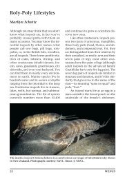
estricted to the localized areas where methane and oxygen are simultaneouslyavailable .Oxygen is present in the ambient seawater, methane from either directevolution of gas bubbles or dissolved in brine (MacDonald et al . 1989) . Mytilid bedsoften define the distinct boundaries of this availability .Living clams are either infaunal, in the case of the lucinaceans, or epibenthic,in the case of the vesicomyids .The latter often form distinctive furrow-like tracksas they plow through the surface sediment in search of sulfide (Fisher 1990) .Areaswhich living vesicomyids occupy more or less continuously may be 100 to 150 m inwidth (Rosman et al . 1987) . The dead shells of both groups, however, tend toaccumulate on the surface sediment, sometimes producing shell "pavements" thatcover more extensive areas (Callender et al . 1990) . The shells of the two groups areoften difficult to distinguish from each other visually and dead vesicomyids oftenoccur in life position .Visual observations of shell beds may therefore indicate acommunity of living vesicomyids or an infaunal community of lucinaceans .2.3 Zonal Distribution of Chemosynthetic Communities in the NorthernGulf of Mexico2 .3 .1 Local PatternsThe best evidence for long-term seepage is presence of chemosynthetic faunaat specific sites .Figure 2.1 shows the locations where the major chemosyntheticfauna have been collected or unambiguously observed .Table 2.1 lists the groups ofchemosynthetic fauna found, nominal locations, depths, collection method and thecitation .Occurrence of a chemoautotrophic community can indicate a range ofenvironmental conditions ;in all cases, however, this fauna is an indicator ofhydrocarbon seepage (Brooks et al . 1987 ; Kennicutt et al . 1988a) . Reliability ofinformation on the areal extent, density, and continuity of the individualcommunities shown in Figure 2 .1 is uneven .Clearly, trawl samples will not provide2-3

Table 2.1Sites where chemosynthetic metazoans have been collected by trawl(Trl) or submarine (Sub), or definitively photographed by submarine,remotely operated vehicle (ROV), or photosled (Photosl) . Faunaindicates the type of chemosynthetic fauna found : V=vestimentiferantube worms, M=Seep Mytilids, C=vesicomyid or lucinid clams,PG=pogonophoran tube worms ; codes in bold face followed by asterisk(e.g ., 1* VM) are Sampling Sites for the present study . Lease blockdesignators follow MMS standard abbreviations . Data sources giveprecedence to observations published in the open literature .Fauna Latitude Longitude MMS Depth Obs Data(North) (West) Lease Block (m) method sourceVM 26°21 .20' 94°29.80' AC0645 2200 Sub 1M 27°23.50' 94°29.45' EB0602 1111 1r1 2PG 27°27.55' 93°08.60' GB0500 734 Tr1 2VC 27°30.05' 93°02.01' GB0458 757 ZYl 2M 27°31.50' 92°10.50' GB0476 750 Sub 3MC 27°33.40' 92°32.40' GB0424 570 Sub 3V 27°35.00' 92°30.00' GB0425 600 Sub 3VC 27°34 .50' 92°55 .95' GB0416 580 Sub 3VC 27°36.00' 94°46.00' EB0376 776 Sub 3PG 27°36 .15' 94°35 .40' EB0380 793 Tr1 2MC 27°36.50' 92°28.94' GB0382 570 Sub 3VC 27°36 .60' 94°47 .35' EB0375 773 Trl 2VC 27°36.82' 92°1525' GB0386 585 Sub, Tr1 2,3VC 27°37 .15' 92°14.40' GB0387 781 Sub, Zl-1 2,3V 27°37.75' 91°49.15' GC0310 780 1Yl 2VC 27°38.00' 92°17.50' GB0342 425 Tr1 2C 27°39 .15' 94°24 .30' EB0339 780 Tr1 2VC 27°39.60' 90°48.90' GC0287 994 Sub, Tr1 2C 27°40.45' 90°29.10' GC0293 1042 Tr1 2VC 27°40.50' 92°18.00' GB0297 589 1Y1 2VMC 27°40.88' 91°32.10' GC0272 720 Sub, TYl 2, 3, 4VC 27°42.65' 92°10.45' GB0300 719 Tr1 2V 27°43.10' 91°30.15' GC0229 825 Tr1 2VM 27°43.30' 91°16.30' GC0233 650 Sub 5VMC 27°43.70' 91°17.55' GC0233 813 Tr1 2VM 27°44.08' 91°15 .27' GC0234 600 Sub 3,6VM 27°44.30' 91°19.10' GC0232 807 Sub 3VM 27°44.80' 91°13.30' GC0234 550 Sub 3,7VC 27°45.00' 90°16.31' GC0210 715 Sub 3C 27°45.50' 89°58.30' GC0216 963 Sub, Photosl 8,2VMC 27°46.33' 90°15.00' GC0210 796 Sub 3VM 27°46.65' 91°30.35' GC0184/5 580 Sub, Trl 2, 3, 9VM 27°46.75' 90°14.70' GC0166 767 Sub, Tr1 2,3VM 27°49.16' 91°31.95' GC0140 290 Sub 10V 27°50.00' 90°19.00' GC0121 767 Sub 3VM 27°53.56' 90°07.07' GC0081 682 Photosl 11VC 27°54.40' 90°11.90' GC0079 685 Tr1 2VM 27°55.50' 90°27.50' GC0030 504 Sub 3VPC' 27°56.65' 89°58.05' GC0040 685 Trl 2C 27°57.10' 89°54.30' MC0969 658 Tr1 2V 27°5725' 89°57.50' EW1010 597 Sub, 1r1 2,3V 27°58 .70' 90°23 .40' EW1001 430 Sub, Tr1 2,3VC 29°11 .00' 88°00 .00' VK0826 545 Sub, R.OV, Tr1 3, 4, 12Data sources: 1-Brooks et al . . (1989), 2-Kennicutt et al . (1988a,b), 3-GEftG unpubl . data, 4-Callender et al .(1990), 5-MacDonald et al . (1990b), 6-MacDonald et al . (1990b), 7-MacDonald et al . (1990a), 8-Rosman et al .(1987), 9-MacDonald et al . (1989), 10-Roberts et al . (1990), 1 1-Boland 1986, 12-Boss (1968), Gallaway et al .(1990), Volkes (1963) .2-4

981W 96°W 94°W 92°W 90°W 88°W 860W32oN i30°NVK 82628°N-------------200- 1000 m26°NIOOOT __ . ., --_,____ ` 3000 m,Figure 2 .1Locations where vestimentiferan tube worms, seep mytilids, or vesicomyid clams have been collected orphotographed in the northern Gulf of Mexico . Observations separated by less than 1 NM have beenpooled . Study sites are indicated by their MMS lease block number.

eliable data of this type ; and photo surveys generally cannot provide an exhaustivemapping of individual communities . It is therefore difficult to determine whatconstitutes a chemosynthetic community in terms of management concerns . Does,for example, a single collection of clam shells signify a lush community? Likewise,in how much detail should offshore operators be required to search in order tocertify that their operations will not impact a lush community? One approach tothis issue is to examine the variable evidence for the typical length scales andgeological dependency of well-documented chemosynthetic communities .An analysis of clustering frequencies for tube worms at GC 234 foundsignificant clustering at spatial scales of about 5, 20, and 75 m (MacDonald 1990a),which may be indicative of clustering due to formation of tube worm "bushes" at thesmaller scale, and to the size and spacing of fault zones at the larger scales .Areview of the occurrence of chemosynthetic fauna along the submarine track-linestends to confirm a characteristic size of 10 to 100 m for vestimentiferan and mytilidcommunities and 100 to 300 m for clam communities .We therefore have supportfor speculation that communities separated by less than 300 m probably share acommon hydrocarbon reservoir. Multi-channel seismic data from the GC 184/185lease blocks (Cook and D'Onfro 1991) provided information on the spacing ofreservoirs and migration pathways at this site .From these data, it appears thatcommunities separated by distances of 1 km are not supported by seepage from acommon reservoir.2.3.2 Regional PatternsChemosynthetic fauna have been found in a 700 km-long corridor between88°W and 95°W and between the 290 and 2200 m isobaths . Distribution is uniform ;the greatest number of communities were found between 91°W and 93°W betweenthe 500 and 700 m isobaths .These observations have been influenced by the limits2-6

of exploration; the envelope of occurrence suggests that the potential number ofcommunities is much larger than those found to date . There was a gap inoccurrences where the Mississippi Canyon intersects the corridor . Although thisarea has not been exhaustively explored for communities, geochemical explorationshows a general absence of oil-stained sediments from the Canyon, which suggeststhat the hiatus in community occurrence may be real (GERG unpublished data) .The easternmost community, in the Viosca Knoll block 826, was found byinvestigations initiated by the Orb Energy Company (Gallaway et al . 1990) .Interestingly, this area was trawled in 1955 by the U.S .Fish and Wildlife Service'sMN Oregon .The resulting collections provided the holotype for the originaldescription of Calyptogena cordata (Boss 1968) and a paratype for the originaldescription of Acesta bullisi (Volkes 1963) .The photograph of this paratype showsthe unmistakable shell deformation that is caused by the commensal interactionwith a vestimentiferan .The Viosca Knoll site represents early, unrecognizedevidence for hydrocarbon seep communities in the northern Gulf, as well as a recentrange extension.Each chemosynthetic community supported by hydrocarbon seepage dependson a reservoir of hydrocarbon and a migration pathway or pathways through whichthese fluids reach the seafloor . Implicit in the distribution shown in Figure 2 .1, orin a larger scale mapping of community distribution, is a determination of whatspatial separation is required to consider two occurrences as distinct communities .The number of communities in a given area should be indicative of the number ofhydrocarbon reservoirs, the number of migration pathways (i .e ., faults), thecharacteristic size of the faults, and interaction of the unconsolidated sediments,hydrates, or carbonate with seepage . This determination is also important forestimating the numbers of the communities and for management concernsregarding the potential zone of impact for a seafloor activity .2-7

2.4 Remote-Sensing Detection of Natural Oil Seepage2.4.1 Use of Geophysical Methods for Indirect Detection of ChemosvntheticCommunitiesOur study suggests that geophysical techniques can be used to narrow theareas of detailed study needed to locate and classify chemosynthetic communities.Ultimately, no geophysical method will allow the reliable identification of suchcommunities without in situ observation .However, by using known geophysicalsignatures and affinities, likely locations can be identified for more detailed study .Seeps are located along faults and faults are usually identified in regionalseismic exploration profiling surveys .Thus, the first step in locatingchemosynthetic communities is to map the faults along which seeps could occur .The likeliest faults to harbor seeps are those that are active and thus extend to thesurface and those that show a significant displacement .Having found the faults, the next step would be to look for seep relatedtopography and sediment disturbance . Topographic features would be mudmounds, carbonate mounds, and pock-marks . The mud mounds are typically morethan 10 m in height and more than 100 m in diameter and would be evident onhigh-resolution bathymetry maps and side-scan sonar images . Carbonate moundscan be somewhat smaller, one to a few meters high and 10 m wide, or less . Inaddition, pock-marks are variable in size, from small, shallow craters a few metersacross to large craters many meters deep and hundreds of meters wide .Sediment disturbances can usually be found using acoustic profiling andimaging techniques . On side-scan sonar records, the disturbance can appear as anincrease in backscatter, particularly in conjunction with small mounds . In 3 .5 kHzand other echo sounder profiles, the disturbance may show up as an attenuation ofsignal reflections ("wipe out"), as an enhancement ("hardbottom"), or as2-8

everberation ("turbidity") .These are caused mostly by gas, carbonate layers ordisseminated nodules, or hydrate layers .In addition, if the seepage is particularlystrong and contains much gas, the gas bubbles may be detected within the watercolumn by these acoustic methods (Anderson and Bryant 1990) .Having located areas of larger scale topographic features or sedimentdisturbances caused by seepage, a more detailed examination is necessary .Tolocate chemosynthetic communities, various ultra-high-resolution imaging methodsare needed .Side-scan sonar images will show carbonate outcrops, and may evenshow tube worm bushes or bivalve clusters if the resolution is high enough and theorganisms are dense enough .Typically, this will require a deep-towed sonar orsonar affixed to a submersible, so that the acoustic source and target are not greatlyseparated .invisible .However, many chemosynthetic organisms, such as bivalves, may beUnderwater photography, such as with a camera sled or a laser line-scandevice can provide visual sitings, as can submersible dives .Although these last areslow and painstaking techniques, presumably they can be directed, using a nestedsearch technique employing increasingly higher resolution methods, so that thetime consuming visual searches can be minimized .Likewise, new technologies,such as laser line-scanning imaging, may dramatically improve the search speed forvisual survey .Another nesting procedure would combine geophysical methods withremote sensing of floating oil by use of airborne or satellite sensors .2.4 .2 formation and Detection of Surface Oil SlicksOil, and other organic compounds, can be detected remotely in the oceanbecause they form a floating film that modifies the characteristics of the surfacelayer and locally increases specular reflection of radiant energy such as visible lightor radar waves (Garrett 1986 ; Scott 1986 ; Stevenson et al . 1988) . The phenomenonhas been used to study small-scale oceanographic circulation (Cox and Munk 1954 ;2-9

Soules 1970 ; La Violette and Arnone 1988), the effects of ship wakes (Peltzer et al .1992), and the surface slicks formed by natural oil seepage (Estes et al . 1985) .Micro-layer surfactants originate from at least two sources : petroleum oil and thebiological activity of plankton and fish (Garrett 1986) . Although biologicalsurfactants are physically and chemically different from oil, and can bedistinguished remotely by their wave damping properties under some circumstances(Huhnerfuss et al . 1989), confirming the source of a remotely detected micro-layer isoften difficult or impossible . By comparing remote sensing images that showevident oil slicks with locations of chemosynthetic communities (Table 2.1) andsurface observation of floating oil (MacDonald et al . 1993) made it possible toconfirm the locations of perennial oil slicks from natural seepage .2 .4 .3 Remote Sensing MethodsThe remote sensing data base comprised images collected from three sensorsystems on board three satellites :1) European Radar Satellite (ERS-1, SAR, image)Orbit Frame Date9518 3051 8 May 19939475 3051 8 May 199311250 3051 9 Sept . 19932) Landsat - (Landsat 5, Thematic Mapper image)Path, RowCollection Time and Date22,41 1105 CST 31 July 19913) Space Shuttle (Atlantis with 120 mm format photograph, hand-held)Mission, Roll, and Frame Collection Time and DateSTS-30, 151, 028 1535-1538 CST ; 05 May 19892-10

The Space Shuttle photograph was scanned and digitally resampled toconform with the position of known coastal features and offshore installations .Suspected slicks in these images were outlined as closed polygons .The set of slickpolygons for each image was then stored as a layer in a geographic informationsystem (GIS) by use of MAPIX@ software .The objective of this exercise was to combine observations from the data setsdescribed above, then to review these observations to identify probable sites for seafloorseeps . This was accomplished in a 2-stage fashion: First, all possible imagepairs were compared to determine co-locations of slick polygons . Overlappingpolygons were classified according to the style of conjunction by use of the followingranking scheme :Rank A : Overlap of the upwind ends of slicks in two or more images .Rank B : Overlap of slick ends irrespective of wind direction .Rank C : Ends of slicks within =2 km of each other .Rank D : Overlap of any portion of slick polygons in two or more images .Second, slick polygons were compared to locations of collections of floating,freshly surfaced oil and to locations of chemosynthetic communities .A location wasconsidered to be a geochemical anomaly if a visibly oil-stained sediment sample wascollected in the same lease block with a surface slick or community ofchemosynthetic animals .By analyzing the remote sensing and ancillary data, we found 63 locationswhere multiple data sets indicated presence of perennial oil slicks (Table 2 .2, Figure2 .2) . At six of these sites, we report collection of freshly surfaced oil from thesurface at locations that coincide with a target in one of the remote sensing images .Oil-stained sediments and chemosynthetic fauna were also present in five and three2-11

Table 2.2Oil slicks detected in one or more remote sensing images from thenorthern Gulf of Mexico . Latitude and longitude are for point ofoverlap . Lease block designators follow standard MMS format .Depths given are mean depths for lease block . Slicks listed as havingno overlap were confirmed by coincidence with sea truth collections orobservation from submarine .ID Latitude Longitude Lease Depth Remote Sensing Seafloor Geoc emits Floating iBlock (m) Overlap Manifestation Anomaly Collected1 27044.83'N 91013.33'W GC0234 831 no overlap Chemo fauna Oily core Floating oil2 27043.71'N 91036.57'W GC0226 825 no overlap - Oily core Floating oil3 27040.53'N 92018.00'W GB0297 589 no overlap Chemo fauna Oily core Floating oil4 27031.55'N 92010.58'W GB0476 891 no overlap Chemo fauna - Floating oil5 27021.99'N 92023.01'W GB0648 1058 no overlap - Oily core Floating oil6 27013.02'N 91003.12'W GC0766 1523 no overlap - Oily core Floating oil7 27057.88'N 90043.23'W EW0995 281 upwind ends - - -8 27055.63'N 91052.86'W SM0205 184 upwind ends - Oily core -9 27048.73'N 90051 .03'W GC0154 715 upwind ends - Oily core -10 27048.65'N 91007.20'W GC0148 551 upwind ends - - -11 27045.04'N 91029.48'W GC0229 825 upwind ends - - -12 27042.74'N 91019.14'W GC0232 807 upwind ends - Oily core -13 27040.52'N 90049.46'W GC0287 994 upwind ends Chemo fauna* - -14 27038.93'N 90048.39'W GC0331 1037 upwind ends - - -15 27037.26'N 91017.38'W GC0321 881 upwind ends - Oily core -16 27033.29'N 90058.55'W GC0415 1049 upwind ends - -17 27°32 .55' N W60 .00' W GC0415 1049 upwind ends - - -18 27032.10'N 90059.75'W GC0415 1049 upwind ends - - -19 27032.04'N 91024.65'W GC0451 1027 upwind ends - - -20 27031.96'N 91023.18'W GC0451 1027 upwind ends - Oily core -21 27031.41'N 91022.31'W GC0451 1027 upwind ends - - -22 27027.12'N 90055.64'W GC0504 1181 upwind ends - - -23 27°24.89' N 91022.67W GC0539 1288 upwind ends - - -24 27024.53'N 91021 .86'W GC0540 1307 upwind ends - - -25 27024.12'N 91039.70'W GC0577 1274 upwind ends - - -26 27023.88'N 91021 .05'W GC0584 1375 upwind ends - - -27 27°22.70' N 91045.02'W GC0576 1302 upwind ends - - -28 27022.56'N 91010.25'W GC0588 1502 upwind ends - - Floating oil29 27022.32'N 91010.45'W GC0587 1558 upwind ends - - -30 27021.39'N 91003.09'W GC0590 1404 upwind ends - Oily core -31 27021.31'N 90002.97W GC0611 1341 upwind ends - Oily core -32 27017.97'N 91011 .95'W GC0675 1622 upwind ends - - -33 27014.35'N 91036.36'W GC0711 1412 upwind ends - - -34 27°13 .98' N 90054.12'W GCO725 1455 upwind ends - - -35 27013.62'N 91001 .21'W GC0723 1421 upwind ends - Oily core -36 27Q13.56' N 90047.80'W GC0727 1374 upwind ends - Oily core -37 27012.41'N 91002.04'W GC0766 1523 upwind ends - Oily core -38 27005.60'N 91021.69'W GC0892 1999 upwind ends - - Floating oil39 27°05.09' N 91023.75'W GC0891 2006 upwind ends - - -40 27044.24'N 91°18.83' W GC0232 807 ends undeter . Oil seep obs. Oily core Floating oil41 27042.74'N 91019.14'W GC0232 807 ends undeter . Chemo fauna Oily core -42 27°31.35' N 91024.25'W GC0451 1027 ends undeter . - - -43 27015.05'N 91035.83'W GC0711 1412 ends undeter . - - -44 27013.76'N 91002.02'W GC0722 1414 ends undeter . - Oily core Floating oil45 27013.57'N 90048.89'W GC0727 1374 ends undeter . - Oily core -46 27048.51'N 90051.07W GC0154 715 ends < 2km - - -47 27039.64'N 91022.03'W GC0319 909 ends < 2km - - -48 27024.73'N 91018.44'W GC0541 1374 ends < 2km - - -49 27010.42'N 91012.36'W GC0807 1676 ends < 2km - Oily core -50 27047.63'N 91007.23'W GC0148 551 random overlap - - -51 27046.67'N 91030.39'W GC0185 718 random overlap Oil seep obs. Oily core Floating oil52 27044.47'N 91012.75'W GC0235 841 random overlap - Oily core -2-12

53 27043.62' N 91026.19'W GC0230 825 random overlap - - -54 27040.93'N 91°36.46' W GC0271 851 random overlap - Oily core -55 27032.79'N 90058.34'W GC0416 1072 random overlap - - -56 27032.60'N 91032.67'W GC0404 947 random overlap - Oily core -57 27028.39'N 90066.73'W GC0504 1181 random overlap - - -58 27027.09'N 90064.70'W GC0505 1172 random overlap - - -59 27026.18'N 91050.52'W GC0530 1176 random overlap - - -60 27022.43'N 91021.62'W GC0584 1375 random overlap - - -61 27020.55' N 91023.44'W GC0627 1395 random overlap - - -62 27°18.90' N 91038.93'W GC0666 1323 random overlap - - -63 27018.13'N 91010.80'W GC0675 1622 random overlap - - -cases, respectively .At 39 sites listed in Table 2.2, we make our primarydetermination based on overlap of the evident upwind ends of slicks in two or moreof the remote sensing images .Floating oil was collected at two of these sites andoil-stained sediments were collected at an additional ten sites within this group .Among the remaining 23 locations listed in Table 2 .2, four are distinguished asparticularly strong candidates for perennial seeps because of positive indicatorsamong the supporting data sets .The remaining sites fit into our scheme ofoverlapping targets in multiple remote sensing images, but they lack supportingevidence .Three locations were selected for dives with the research submarine JohnsonSea-Link because they coincided with remotely detected oil slicks .The dives hadthe objective of trying to locate a chemosynthetic community or other definitiveevidence for long term seepage on the sea floor below each surface target .Inparticular, the concern was to explore potential new sites that were in greater waterdepths than previously known sites . All dives were made with the researchsubmarine Johnson Sea-Link, which has a maximum depth rating of 1000 m.Johnson Sea-Link was supported by the mother ships R/V Seward Johnson and RNEdwin Link . Dives consisted of approximately 2 h of bottom time ; during which, thesubmarine was first directed to the appropriate location by a surface ship, thencarried out autonomous exploration based on what was visible to scientists in thesubmarine .2-13

92 9128v.rRtIJN. 1,.-T 1~7iLI4v-. ERS1 11250, 1993 50 km .Space Shuttle LFC, 1989figure 2.2ERS1 11551 8851, 1993 Landsat TM, 1991Overlap between oil slicks detected in remote sensing images from different dates reveals the locations ofperennial oil seeps . (Rectangular outlines show coverage for individual remote sensing images .) ERS-1:European Radar Satellite 1, TM : Thematic Mapper, LFC : Linhoff Frame Camera .

Sites selected for dives were located in the Green Canyon 232, 287 and 321lease blocks (Table 2.2) .We were able to find chemosynthetic fauna at the first twoof these sites, but not at the third .The surface slick in Green Canyon 232 wasspotted from an airplane and was clearly visible to ship-board observers before itwas noted in the satellite data .During two dives to depths of 700 m, we noteddense aggregations of tube worms and seep mussels similar to assemblages at theBush Hill site (MacDonald et al ., 1989) .One of us (Guinasso) inadvertently causeda copious discharge of oil and gas from the sea floor by attempting to collect some ofthe mussels . The mussels were clustered within a field of authigenic carbonaterubble . Probing the mussel cluster with a scoop sampler disturbed the carbonatesubstratum and initiated a burst of gas bubbles followed by a flow of oil dropletsthat continued unabated for over 30 min . Arrival of the oil droplets at the surfacewas noted by the shipboard observers at a location about 100 m from thesubmarine's sea floor position .The surface slick at Green Canyon 287 was noted in the LandSat TM andERS-1 data sets . The site is the location is on a plateau that rises from a base depthof 1500 m to a crest depth of 760 m . A salt body has intruded to the near seafloorand salt movement has produced a series of shallow faults trending northwestsoutheastnormal to the salt (see Reilly et al ., this volume) . The Johnson Sea-Linkbottomed at a depth of 800 m and followed a southern course across the flank of theuplift block . This track took the submarine across a series of northwest-southeasttrending valleys . Clam shells, carbonate outcrops encrusted with tube worms, andoccasional gas seeps were observed in the floors of these valleys . Although clamshells were broadly distributed, the abundance of chemosynthetic fauna in thecommunities at this site was much less than at the Green Canyon 232 site .Although gas venting was evident at several locations, macro-seepage of oil was not2-15

observed .Extractable hydrocarbons from sediment samples at the site were heavilybiodegraded (MacDonald, unpubl . data) .Surface slicks at the Green Canyon 321 site were evident in all of the remotesensing data sets .We traversed the sea floor below these slicks repeatedly duringmore than 6 hours of submarine exploration that covered depths from 750 to 900 m.Occasional indications of oil seepage, i.e .mats of Beggiatoa bacteria and outcrops ofauthigenic carbonate, were observed, but neither significant aggregations ofchemosynthetic fauna nor other definitive sea floor indications of macro-seepagewere observed .2 .4 .4 Estimates of Total SeepageEstimating the magnitude of seepage required to produce slicks of a givenlength requires knowledge of the detectable thickness of the visible oil slick, the rateat which it advects away from the point at which the oil arrives at the surface, andthe rate of disappearance due to evaporation and dissolution .Direct measurementof slicks over oil seeps suggests slick thicknesses of 0 .1 to 1.0 ~tm (Allen et al . 1970) .Duckworth (personal communication 1993) dispensed a variety of crude oils onseawater and observed the coverage .Although results depended upon oil type,water cleanliness, and evaporation, generally 1 ml of oil will spread to produce astable silver-gray film that covers 10 sq m, which corresponds to a mean thicknessof 0.1 gym .The stable film degraded to an invisible film that suppressed capillarywaves and enhanced reflectivity, and that occupied an area consistent with athickness of approximately 0 .01 gym .Slick thicknesses required to produce therainbow sheen and mousse reported during the sea-truth trials probably exceeded 1gm ;however, these observations were restricted to small areas within the overallslicks, and the slicks themselves contained patches of un-oiled water.A thicknessof 0 .01 gm is therefore a reasonable lower limit for a detectable slick .2-16

Oil floating on the sea degrades as a result of evaporation and dissolution .Asa slick disperses from its point of origin, these effects will compound progressivethinning of the slick due to spreading until the slick is no longer detectable(Hollinger and Mennella 1973).A slick formed by an instantaneous release of oilwill therefore have a set detectable life span .A persistent slick represents acontinuous flux of oil to the surface (Fallah and Stark 1976).Oil coming to thesurface continuously into an advective regime caused by current or wind forms aplume.An advective velocity of 20 cm sec-1 would move oil downstream from apoint at about 17.2 km day-1.Plumes with lengths of the order of 5 km contain oilthat has been on the surface for less than 1 day . Hollinger and Mennella (1973)noted that the oil slicks are thickest along a central axis and suggested that most ofthe oil in a slick is confined to a small fraction of its total area .More about the nature of these plumes can be learned by proposing a simpledispersion model of a plume . We posit a Gaussian distribution of oil thickness inthe transverse cross-section of a plume because this is consistent with previousfindings and because analytical solutions to Gaussian functions are well-described .A three-dimensional Gaussian plume can be described byc = q ex -rx _ y22n u a ~ u 2a2 (1)where c is the thickness of the oil on the surface, cm ;q is the seafloor seepage rate,cm3 sec-1 ; u is the advection velocity, cm sec-1 ; x is the downwind distance, cm ; r isa degradation coefficient for the oil, sec-1 ; y is the cross plume distance, cm ;and s isthe cross plume standard deviation .The standard deviation is given by assumingdiffusion-like spreading so that= 21~dx /u (2)2-17

where x is downwind distance, cm ; and d is a dispersion coefficient, cm2 sec-1 .Similar models are described by Csandy (1972) to describe a plume resulting from acontinuous oil spill .The x,y points that lie on the boundary of the detectable plume satisfy theequation9ex -rx _ y 2 -cd = 02n u a 4 u 2a2 ~ (3)where cd is the minimum detectable thickness of oil, cm ;r is the e-folding time ordegradation constant (r = 0 .693/(86,400T), sec-1 ; T is a degradation half life, days ;and s is given by (2) .The model requires that the size and shape of the detectableplume is dependent on the parameters q, cd, u, r, and d, which we will refer to asthe parameters .Some insight can be gained into these equations by scaling them interms of some simple dimensionless variables .A natural scale length for theproblem is given byL=du (4)Substituting the dimensionless variables Y=y/L, X=x/I., R=rd/u2, and Q=q/(dcd) into(1) giveszC=1 Q exp(-RX - )(5)2-18

When Y, the dimensionless crossplume distance equals zero, thenC = 2 Q exp(-RX)(6)The length of the plume is that value of X defined by (6) when C=c/cd = 1 .Substituting C=1 into (6) we can solve for Q as a function of the overall length of theplume XLQ = 2-~rn-XL exP(RXL) (7)The shape of the plume is given by solving (5) for Y with C=1 .This givesY = 2-1X -lnQexp(-RX)We estimated the range of possible seepage rates required to produce theslicks in the two images by solving (7) for the lengths of slicks measured in theShuttle and TM images .We used an advection rate, u = 20 cm s-1, which weestimate from the recorded wind speeds, and threshold thicknesses, cd = 0.01 and0.1 gym, and degradation half-life, T = 0 .25 and 1 day, which we regard as areasonable range for these parameters .This exercise suggests that natural seepageis on the order of 4.3 x 103 to 7 .8 x 104 m3 y-1 in the 8,200 sq km area imaged in theTM scene and 1.1 x 104 to 4 .8 x 105 m3 y-1 in the 15,000 sq km area imaged in the1989 Atlantis photograph .2-19

2 .4.5 trial of the Laser Line Scan SystemAt present there are two means for sea-floor imaging:seismic and optical.Seismic imaging, such as side-scan sonar or active sonar, is distinctly limited inresolution .Optical imaging, such as underwater photography, has long beenlimited in scope because of backscatter.The Laser Line Scan System (LLSS) is astate-of-the-art optical imaging system that overcomes the back-scatter problemsplaguing underwater photography .Very recent design improvements byWestinghouse Electric Corp ., Underwater Laser Systems have produced a newLLSS, Model SM2000S, that reduced power requirements to under 200 watt andreduced size and weight by roughly half.This improvement makes this LLSS apotential tool for much of the research submersible fleet including ROV's and towedfish, but as yet, the submarine user community has not undertaken any detailedscientific or engineering tasks with the system .In its current configuration, theLLSS provides high-resolution pictures of the seafloor along swaths up to 40 mwide .Despite the promise of this technology, it was unclear whether it could beused to image chemosynthetic fauna in adequate detail .A modification to the Study program was made to facilitate a trial with alaser system over Bush Hill . In this trial, the ART laser system, operated by SAIC,diverted from another mission and spent 12 hr surveying the GC 184 study site .This laser system was deployed in a towed fish by the RN Gyre . The laser producedexcellent images in shallow water, but was severely limited by tow-fish stability indeeper waters . The results over Bush Hill were, therefore, disappointing in terms ofproviding a detailed map of the community. The effort did produce several quitesatisfactory images of tube worm clusters and bacterial mats (Figure 2 .3) . Thisdemonstrates that the technique can work, provided the stability problem is solved .2-20

Figure 2.3 Laser line scan image collected over Bush Hill during the June 1993trials . Note the extreme image distortion caused by the roll, pitch andyaw in the towed vehicle . During a brief intervals of relative stability,the instrument captured a very clear image of several tube wormcolonies . The largest colony is probably 1 to 2 m in diameter . Note thevery abundant white patches of bacterial mats .2.5 SummaryChemosynthetic fauna occur across most of the continental slope in thenorthern Gulf of Mexico .Their distribution is more homogeneous over largergeographic and depth ranges than is the case for hydrothermal vent communities .Seep communities tend to be dominated by vestimentiferans, seep mytilids, orvesicomyid and lucinid clams, but intergradations among these community typesare the rule, particularly between vestimentiferans and mytilids . The MMSChemosynthetic Ecosystems Study encompasses a series of study sites which were2-21

selected from the known list of communities on the basis of community type andgeographic location .Methods for the remote sensing of chemosynthetic communities, many ofwhich were developed or refined during this Study, can be applied to improveunderstanding of the distribution of hydrocarbon seepage . The distribution ofmacro oil seepage revealed by satellite remote sensing demonstrates that theconditions required for formation of hydrocarbon seep communities extend wellbeyond the artificial limits imposed by the exploration tools previously used . It isquite defensible to assume that hydrocarbon seep communities occur to depths of2000 m or greater across much of the northern Gulf of Mexico slope .2-22

3.0 Geological and Geophysical Characterization of HydrocarbonsWilliam W . Sager, Changshik Lee, and William W . Schroeder3 .1 IntroductionHydrocarbon seeps have been routinely studied by the oil industry usinggeophysical techniques .Often the deep subsurface structure is known throughmultichannel seismic reflection profiles acquired to find oil .Also, in areas wheredrilling rigs or pipelines are to be located, the oil industry has often acquired highresolutiongeophysical data for a "hazard" survey .Even the most precise of highresolutionsurveys, however, has insufficient resolution to image objects on scales of afew meters because of the separation of the observer at the sea surface from thetarget on the seafloor .Thus, small features and biologic communities at seeps arenot routinely imaged by traditional sea surface geophysical techniques .In contrast, much of our knowledge of the biology or geochemistry ofhydrocarbon seep communities comes from either dredge or trawl samples, orsubmersible viewing and sampling .Dredges and trawls provide spot samples, but areoften difficult to relate to the seafloor in detail because they are typically dragged overthe seafloor .Submersible studies provide a detailed view of the communityinhabitants, relations, and small scale distribution, but are limited in scope byvisibility and the slow speed at which observers can traverse the seafloor in asubmersible .What is missing in this spectrum of studies is a link from the broad scale ofgeophysical sounding to the ultra small scale of the submersible viewport .In thisreport we examine the use of a hybrid technique, geophysical data collected from asubmarine, as the basis of a study of the geological and geophysical characteristics ofhydrocarbon seeps in the Gulf of Mexico .These geophysical data provide a synoptic3-1

view on the scale of hundreds of meters, but with a resolution of less than a meter andthis allows us to compare viewport-scale observations with broad scale seismic data .Our primary observations were made with two acoustic tools, a 25 kHz echosounderand a 77 kHz side-scan sonar. Both were used aboard the U.S . Navy nuclearsubmarine NR-1 to collect profile data in grids over four hydrocarbon seeps known tobe inhabited by chemosynthetic communities.We chose these particular seepsbecause they have been the subject of intensive interdisciplinary studies and industrygeophysical data are also available for all to some degree .This situation allowed us toexamine the middle scale geologic characteristics and to link the ultra small and broadscale data sets .In this report, we attempt to synthesize the geological andgeophysical characteristics of each of these four sites and then extrapolate thisinformation to the broader population of chemosynthetic community sites .3.1 .1 Study LocationThe four seep sites examined in the geological/geophysical study are all locatedon the Louisiana continental slope in the Green Canyon (GC) and Garden Banks (GB)lease blocks areas (Figure 3.1) . From east to west, the sites are GC234, GC 184/185,GB 386/387, and GB 424/425 (for brevity, we henceforth refer to the last three sitesas GC1 184, GB 386, and GB 425) . GC 234 is located along a portion of a tensionalfault between salt diapir ridges (Behrens 1988) . The other sites are all moundslocated either on the flank of a salt diapir (GC 386, GB 425) or on a fault radiatingfrom a salt diapir (GC 184) . The deepest seep site is GB 425 at 575 m, next is GB386 at 585 m, GC 184 at 540 m, and the shallowest is GC 234 at depth of 530 m .3 .1 .2 Geologic Causes and Symptoms of Hydrocarbon Seeps in the Gulf of MexicoHydrocarbon seeps are widely scattered throughout the ocean basins becausethe two main ingredients that give rise to seeps, hydrocarbon source sediments and3-2

51'wgaysz4ow 9?20W 9TiQYY MOW 9190VY91'20W 91'10'W-118'00112T`,iON4T101110 Infigure 3 .1 Location of study areas .3-3

tectonic fracturing, are relatively common (Hovland and Judd 1988) .In the Gulf ofMexico, the source layers are Cretaceous carbonate sediments and Cenozoicterrigenous sediments, both of which have layers containing abundant organic matterthat can form hydrocarbons .Early in its history, during the Jurassic Period, the Gulf of Mexico was ashallow, periodically desiccated basin in which an extensive evaporite layer (theLouann Salt), up to several kilometers in thickness, was deposited (Buffler et al .1980 ; Worrall and Snelson 1989). Many additional kilometers of sediment, firstcarbonate and then terrigenous were piled atop the evaporites, as the basin marginsaged and subsided (Worrall and Snelson 1989 ; Wu et al . 1990a) . The organic materialin these sediments was compressed and heated to form gas and oil .Salt is the mainconstituent of the evaporates .Because it is nearly incompressible, its densitychanges little with burial whereas the overlying sediments become denser throughcompaction .time scales .Moreover, under differential stress, salt deforms plastically on geologicThe end result is that with continuing burial, the Louann Salt becamemobile beneath the Gulf of Mexico shelf and slope during the Cenozoic Era.The mobile salt has greatly affected the physiography of the northern Gulf ofMexico (Jackson and Seni 1983 ; Jackson and Galloway 1984 ; Jackson and Talbot1986 ; Wu et al . 1990b ; Simmons 1991) . It has moved vertically to form diapirs andridges, only some of which have reached the surface .salt nappes and intraslope salt-withdrawal basins .It has moved laterally to formOf greatest significance forchemosynthetic ecosystems, the movements have caused faulting, which is activetoday at many locations .The faults are typically tensional, listric, growth faults,often with parasitic antithetic faults (Worrall and Snelson 1989 ;Seni and Jackson1992) . These faults frequently tap reservoirs of hydrocarbons deep within thesediment column .Not only to they break the reservoir seal, but they also provide aconduit for upward hydrocarbon migration .Thus, hydrocarbon seeps are associated3-4

with active salt movement and active faulting. Because the hydrocarbons cannotpenetrate impermeable hemipelagic muds to any great degree, seeps are found alongthe faults that liberated the hydrocarbons (Roberts et al . 1990) . Moreover, becauseit is the salt movement that causes the faults, usually seepage is on faults near saltbodies (Behrens 1988 ; Roberts et al . 1990 ; Kennicutt and Brooks 1990) .3.1.3 Geophysical Signatures of SeensFor some time it has been realized that hydrocarbon seepage at the seafloorhas effects that can be recognized by acoustic profiling and imaging methods(Hovland and Judd 1988) . The effects can be generally broken into two categories :those that cause some sort of topographic feature and those which change theacoustic reflection characteristics of the sediments .Seep-related topographic features range from depression to uplift . The latterinclude mounds of authigenic (i .e ., formed in situ) carbonate (Roberts et al . 1990) ormud mounds (Hovland and Judd 1988 ; Neurauter and Bryant 1990) . Authigeniccarbonate mounds are formed by precipitation of carbonate during microbialdegradation of hydrocarbons, whereas the mud mounds were probably formed by fluidmud entrained by the ascending hydrocarbons (e .g ., Figure 3.2) . The negativetopographic features are pockmarks (small, subcircular, shallow craters) or blow-outcraters, probably formed by escaping gas (Hovland and Judd 1988) .The acoustic effects of hydrocarbon seeps are several . Gas bubbles within thesediment column can attenuate the acoustic signal, preventing further penetrationand causing a "wipe out" zone in which deeper layers are hidden (Behrens 1988 ;Anderson and Bryant 1990) . This signature can also be caused by near-surfacebiogenic gas, so it is not necessarily a sign of deep-rooted seepage . Authigeniccarbonates change the reflection characteristics of the sediments, causing areverberation or "turbidity" owing to the scattering of sound energy by disseminated3-5

0bba~.00~.a~.0m0NMNM3-6

nodules (Behrens 1988) .This may also be the source of strong acousticbackscattering sometimes seen around seeps using side-scan sonars .Gas hydrateswithin the sediment column also change the reflection characteristics .A hydratelayer may attenuate penetrating acoustic waves and it may also cause bottomsimulating reflectors (BSRs) owing to the acoustic impedance contrasts at its edgesHovland and Judd 1988) .3.2 DataAs stated above, the primary data for this study were 25 kHz echo sounderprofiles, 77 kHz side-scan sonar images, and bathymetry data acquired with thesubmersible NR-1 during surveys in 1991-1992 (GC 184/194, GC 234, GB 386) and1993 (GC 425) . Both the echo-sounder and side-scan sonar were mounted on thelower hull of the submarine, which was sailed at an a more-or-less constant altitude of3 to 10 meters above the seafloor, typically at a velocity of 1 to 2 knots . The echosounder records were recorded in analog fashion on videotape and have a verticalresolution of less than 10 cm .Side-scan sonar records were also recorded in analog,on paper records 20 inches wide .The sonar swath width was set at 100 m, and theimages have a resolution of about 0 .5 m. Most surveys consisted of lines spaced 30to 100 m apart, giving more than 100% overlap of the side scan images from adjacenttracks .Although they are related, the side-scan sonar and echo sounder data showsomewhat different aspects of the seafloor characteristics .The echo-sounder sendsan acoustic wave to the seafloor at vertical incidence, so the received energy isproportional to the reflection coefficient of the seafloor and other interfaces (Urick1975 ; Dobrin and Savit 1988) . Some of the acoustic energy bounces back, but therest penetrates into the seafloor, to be reflected by subsurface interfaces (e.g .,sediment layers) or dissipated .Thus, a plot of received energy versus time gives a3-7

picture of the interfaces at which significant acoustic impedance contrasts occur andthese are interpreted as having geologic significance .Many investigators haveemployed the technique known as "seismic stratigraphy", using external and internalreflection characteristics as a scheme for the classification and interpretationsediment layers (Damuth 1975 ; Damuth and Hayes 1977) .Our purpose for the echosounder data was similar .Except at the nadir, acoustic waves from a side-scansonar strike the seafloor obliquely, so the energy that returns to the instrument is notreflected, but is "backscattered" (Urick 1975) .Backscattering depends on manyfactors and chief among them are topography, seafloor roughness, and sedimenttexture (Johnson and Helferty 1990) .Bathymetry data were also collected along submarine tracks, using a high-frequency echo sounder on the bottom of NR-1 .Bathymetric depths were determinedfrom the two-way travel time of acoustic waves emitted and received by the echosounder .Because the distance from the transceiver and seafloor was small, theseparation was calculated using a constant sound velocity .This distance was addedto the submarine depth, determined by pressure sensor, to arrive at total depth.Some NR-1 cruises produced data in the form of audio and video records ofobjects and organisms on the seafloor .These records were of from visualobservations of features seen out the small forward viewing ports on the submarine .Positioning of the NR-1 was accomplished by inertial navigation betweenacoustic fixes from the mothership at the sea surface .Although the surface ship waspositioned with the military Global Positioning System (GPS) satellite navigation,there are unknown errors in the acoustic ranging position of the submarine at fixlocations .Furthermore, currents or inaccurate drift corrections can lead tosignificant horizontal positioning errors between fees, depending on the frequency andquality of fixes .However, comparison of side-scan sonar record overlaps on adjacent3-8

tracks suggests that for most of the data, the navigation for any given survey isinternally consistent on the order of 5 m or less .Geologic ground truth data were provided by 0 .5-m push cores, visualobservations, and video photography obtained with the submersible Johnson Sea-Link as well as 3-m piston cores acquired aboard the RN Gyre . Both the Gyre and themotherships for the Johnson Sea -Link (RN Seward Johnson and RN Edwin Link),were positioned by civilian GPS satellite navigation, with an accuracy of about 30 m .The submersible was positioned relative to the ship by an acoustic ranging system,which was repeatable to a few tens of meters . Although the Gyre's position wastypically well determined, during coring both the ship's drift and currents pushing thecoring wire off vertical can lead to errors in positioning the cores .Sea surface geophysical data were available for all four sites, but these datawere diverse in type and parameters because most were borrowed from industrysources .For GC 184, GC 234, and GB 386, a few industry multichannel seismicreflection profiles were available .Likewise a variable number of hazard surveyprofiles, typically either run with a 3 .5 kHz or similar echo-sounder or a highresolution multichannel seismic system, were also obtained .The navigation methodsused for these surveys were typically unknown, since the data are proprietary, butindustry standards are such that these data probably have navigation accuracies ofless than 10 m.A more serious problem was offsets between different navigationdata sets ; these offsets were sometimes found to be on the order of a few hundredmeters .In such instances, we had to resort to feature-matching to align submarineand sea surface data .We did not acquire industry data for GB 425, but insteadcarried out a 3.5 kHz and 12 kHz echo sounder survey with the RN Gyre .3-9

3.3 ObjectivesThe objective of this study was to use maps of geophysical (mainly acoustic)characteristics of the seafloor and shallow subbottom at hydrocarbon seep sites toprovide a framework for assessing the effects of the seeps on the seafloor and therelationship to chemosynthetic communities .Using the principles of seismicstratigraphy, we wished to classify and map the extent of sediments affected byseepage . Our goal was to ground truth these classifications with geologic data (coresand submersible observations) and to correlate these characteristics with othergeophysical and geologic data . A major objective of this task was to compare thegeophysical framework with locations of chemosynthetic communities, surfacefeatures, and subsurface structures, such as faults . In addition, we wished to use theobservational framework developed in this study for implications about the geologicformation and evolution of hydrocarbon seeps .3.4 MethodsFor each survey, the geophysical data were plotted at the same scale so thatmaps could be made for comparison of features . Bathymetric data were determinedas described above and contoured at 5-m intervals . Where other sources ofbathymetry data were available, the different data sets were compared to quantifyand correct navigation offsets . The additional data were used to fill gaps or extendbathymetry contours outside the submarine survey area .Side-scan sonar records from NR-1 were automatically slant-range and speedcorrected to produce deskewed images in which the along track and cross trackdimensions are nearly the same .The slant-range correction method is internal to thesonar electronics and assumes a flat seafloor .Consequently, significant deviationsfrom horizontal can cause errors in the plotting of features in the images .Sonarrecords were combined to make a mosaic of the acoustic backscatter variations over3-10

each site .The paper side-scan records were electronically scanned as 8-bit gray scaleimages and were manipulated with a computer program (Photo Styler) to matchcommon features on adjacent sonar swaths .This typically required some smalladjustments of line navigation.The resultant image was a mosaic of the backscattervariations for each site .Some of the mosaics have gaps where it was impossible tomanipulate the side-scan records to be consistent with adjacent tracks .This usuallyoccurred at turns and where the submarine stopped or changed velocity in a mannerthat produced inaccurate speed corrections in the records .The 25 kHz echo sounder data were recorded with a video camera on 8-mmvideotape .These images were played on a videotape player and a Macintoshcomputer with video frame grabbing board was used to capture the images digitally .Each image represented only about 2 minutes of data, so longer records wereconstructed by electronically mosaicking adjacent images .As described below, theecho sounder records were classified by reflection characteristics and thesecharacteristics were plotted along navigation tracks and then contoured to fill in thegaps between lines .Where possible, the side-scan images were used to help theinterpolation between lines .For ground truthing, piston cores and push cores (see Tables 3.1 and 3.2) wereused along with visual observations and video data from submarine NR-1 and theJohnson Sea-Link submersible .The piston cores were obtained from a surface shipand examined for geologic features ;samples were also taken for porosity andcarbonate percentage analysis .Push cores were taken using the manipulator arm ofthe Johnson Sea-Link submersible .They were typically 30 to 50 cm in length, if full,and were extruded and examined visually .Video and voice records were used toidentify the locations of chemosynthetic organisms for some surveys .The time of anobservation was noted, so the observation could be plotted versus the submarinenavigation and thus correlated to sediment acoustic character .3-11

Table 3.1 Description of piston cores .Core ID Description Echo CoreType length(cm)GB 386-A Compact carbonate rock layer at the top of the I 225coreGB 386-B1 Empty I 0GB 386-B2 Empty I 0GB 386-C Homogenous mud (no carbonate) VI 230GB 386-D Homogenous mud (no carbonate) VI 230GB 386-55 Carbonate rock layer in the top 50 cm I 182Cracks filled with oilGB 425-A 10 cm gas expansion void II 215Numerous vesicles and black-stained mud abovethe voidGB 425-B Homogenous mud II 230Vesicles in the top 50 cmGB 425-C Homogenous mud with frequent empty spaces II 235Vesicles between empty spacesGB 425-D Carbonate nodules in the top 35 cm IV 212Shell fragments and oil stains throughout the coreGB 425-E Homogenous mud II 240Vesicles in the top 70 cm3-12

Table 3.2 Description of push cores .Core ID Echo Gas Oil Carbona Shell BacterialType to MatGC 184-a II P tr - - -GC 184-b II P P P P -GC 184-c II P P P - -GC 184-d II P - - P -GC 184-e VI - - - - PGC 184-f II P - - P -GC 184-g II P - P P -GC 234-a VI - - - - PGC 234-b VI - - - -GC 234-c III P tr tr - -GC 234-d VI - - - - PGC 234-e III P P tr - -GC 234-f III P tr - - -GC 234-g VI - - - - PGC 234-h VI - - - - -GB 386-a II - - - - PGB 386-b VI - - - - PGB 386-c VI - - - - P(P = present, tr= trace)3-13

To determine the interrelation of deep and shallow structure, faults and deepstructure were interpreted on select multichannel seismic lines and extrapolated tothe near surface .Structure maps were then compared with the side-scan sonar,bathymetry, and acoustic character maps .3.5 Results3 .5 .1 Acoustic Echo TypesEcho sounder records were divided into six classes (Figure 3 .3) based on theamount and type of apparent disturbance of the sediment layers .Descriptions ofthese classifications are as follows :Type 1 :Characterized by a strong reflector at the seafloor and no evidentacoustic penetration into the subbottom .The strong reflector is probably carbonateor gas hydrate at or near the seafloor and has a high reflection coefficient, causingmuch of the acoustic energy to be reflected or attenuated near the seafloor .Type 2 : Shallow penetration with an abrupt termination of acousticpenetration . This signature probably represents a thin layer of mud overlying ahardbottom, such as carbonate or hydrate . It may show areas in which recent mudflows have covered a pre-existing hardbottom .Type 3 . Scattered subbottom echoes without continuous horizontal internalreflectors . Such a pattern probably shows non-layered sediments disturbed by oil,gas, or disseminated carbonate precipitates .Type 4 .Scattered subbottom echoes with indistinct, horizontally-continuousreflectors .This signature probably represents layered sediments disturbed by gas,oil, or carbonate precipitates .Type 5 . Zones in which acoustic energy is abruptly attenuated ; typicallylaterally-continuous features disappear within these zones .Such zones are widely3-14

::~ v^{TYPE 1~s ate`' ~~,;~v.F .r.,. N~r' g i~tif . . lY ' NTYPE 2 b:.4:e% "y N 1 .< .. : : . . .: f :. . . . . . .y . ., ~ °' °~ fTYPE 3!p ;~ ~-srTYPE 49-E:.. . . . .r .:J: : ' . . . .TYPE 5x v " z ~` +~(ssf R,.:. Nf ~~+5 K" N .TYPE 6~~ ~r.FzFigure 3 .3Examples of acoustic echo types seen in 25kHz subbottomreflection profiles .3-15

ecognized as the result of acoustic attenuation owing to scattering or absorption bygas bubbles within the sediments (Hovland and Judd, 1988) .Type 6 . Parallel, continuous subbottom reflectors . These characteristicsdenote normal, undisturbed hemipelagic sediments .3.5.2 Ground TruthIn this section we describe the implications of our ground truth data for theinterpretations of acoustic fades .Our interpretation of the Type 1 hardbottom zonesis based on cores, side-scan images, and submersible observations .Cores withinthese zones were typically short and contained carbonate rocks, usually within theupper 20 cm, as seen for example in core GB 386-A from the seep mound in GB 386(Figure 3 .4) .Side-scan mosaics often showed rough topography in these regions andwhen viewed by submersible, carbonate outcrops were often seen .Type 2 is similar to Type 1, but is a hardbottom covered with a thin sedimentlayer .Such zones usually appeared no different from surrounding sediments whenseen in side-scan images or from a submersible, because of the covering of sediment.Cores taken in these areas, however, showed similar features to Type 1 area cores,but the hard layers were buried below the surface .Push cores from a Type 2 area onthe seep mound in GC 184 typically contained mud with disseminated carbonate, butone had nodular carbonate at its bottom .About half of these push cores showedtraces of oil .Core GC 425-A, from a similar zone on the mound in GB 425, retrievedmuds of two different colors, separated by an expansion void above which were smallvesicles and a band of dark mud (Figure 3 .5) .This core seems to show the boundarybetween two layers, presumably that seen in the echo sounder records .However, thetwo muds do not have sufficiently different properties to cause a strong reflection attheir interface .Instead, the gas expansion features suggest that gas hydrate mayhave existed at the interface, but it evaporated when the core was raised .Thus, the3-16

carbonate rock(diameter 410 cm)light gray-coloredsilt a claysharp color changeG8386-A%Carbonab0 5 10 15 20 25 30 35PorosityX0.45 0 .50 0 .55 0 .60 0 .85 0.70 0.75 0.8050100gray orreddish brown-coloredsift150200epprosi(y9iCarbonatsFigure 3.4Description of Core G:B386-A, from a Type 1 (hard substrate)echo character zone . At right are trends in carbonate percentageand porosity .3-17

%CarbonateGB425-A 0 s 10 1s 20 2s 30 3sPorosity(1 .45 0 .50 0.55 0.60 0 .85 0 .70 0 .75 0 .e00light gray-coloredsift or dayvesicles(diameter

eflector at this location may have been hydrate . The Type 2 geometry suggests ahardbottom buried by a thin layer of sediment and may indicate recent seep-relatedsedimentation . We base this interpretation in part on observations of mudflows andactive mud expulsion from seep vents on the mound in GB 425, where Type 2sediments cover much of the surface .Types 3 and 4 are similar, except for the existence of internal reflectors, whichare likely related to the original deposition of the sediments . Core GC 425-D (Figure3.6) was recovered from a Type 4 zone (Figure 3.7) and it yielded mud permeated withcarbonate nodules, oil stains, and shell fragments . All three components are potentialscatterers of acoustic waves (particularly if the oil is accompanied by gas) and maytherefore be the source of the apparent disturbance of the sediments noted inreflection profiles .We had no core samples of Type 5 acoustic wipeout zones because theyoccurred rarely in our study areas . Nevertheless, this type of acoustic behavior iswidely recognized as the signature of gassy sediments (Hovland and Judd 1988 ;Behrens 1988 ; Anderson and Bryant 1990) .Several cores were obtained from Type 6 zones in the GB 386 and GC 234study areas . These cores contained hemipelagic muds with little evidence ofdisturbance by hydrocarbon seeps and were similarly lacking in shell fragments andauthigenic carbonates . Thus, we interpreted Type 6 as undisturbed hemipelagicsediment .3.5.3 Distribution of Echo TypesWithin the seep areas we studied, the acoustic fades appear in two differentpatterns . The seeps that are characterized by mounds, such as GB 386, GB 425, andGC 184, are characterized by either Type 1 (hardbottom) or Type 2 (buriedhardbottom) over the mound itself (Figures 3 .7, 3 .8, and 3.9) . These two reflection3-19

carbonate rock(diameter upto 8 cm)light gray-colored mudshell fragmentsoil tracesharp contactG8425-0%Carbonate0 5 10 15 20 25 30 35PorosityX0 .45 0 .50 0.55 0 .60 0 .65 0 .70 0 .75 0 .80dark gray-colored mud50shell fragmentsal trace100150200','.e Porosity. . . - %Carbonate IFigure 3 .6Description of Core GB 425-D, from a Type IV (disseminateddisturbance) echo character zone . At right are trends incarbonate percentage and porosity .3-20

Figure 3 .7 . Patterns of acoustic echo types in the GB 425 survey area .Bathymetry contours shown at 5-m intervals . Echo types areexplained in Figure 3 .3 . Letters A- D show piston core locations(see Tables 3 .1 and 3.2) ; the letter V shows active vent locations .3-21

WNNFigure 3.8 Patterns of acoustic echo types in the GB 386 survey area . Bathymetry contours shown at 5-mintervals . Echo types are explained in Figure 3.3 . Capful letters show piston core locations ; smallletter show push core locations (see Tables 3.1 and 3.2) .

WNwFigure 3.9 Patterns of acoustic echo types in the GC 184 survey area . Bathymetry contours shown at 5-mintervals . Echo types are explained in Figure 3 . Also shown are locations of tube, worm bushes andbivalve shells, denoted by filled and open circles, respectively. Lower case letters show the locations ofpush cores (see Tables 3 .1 and 3.2) .

types show that hardbottoms are at or near the surface, owing to active or recentlyactive carbonate precipitation or hydrate formation .The ape 2 signatures mayindicate recent mudflows that have buried a previous hardbottom, as interpretedfrom submersible observations at GB 425 .The typical nearness of the hardsubstrate to the seafloor suggests that with time, the covering of sediments isprobably incorporated into the hard substrate, so that the hard reflector movesupward through the sediment column .Alternatively, erosion may uncover some hardsubstrate .Given the uniformity of the burial or exposure of most hard substratereflections, it seems that the upward movement is probably the most likelyoccurrence .Interestingly, patterns of Type 1 and Type 2 occurrence are slightly differentat each site .GB 386 has Type 1 over the mound summit and Type 2 around its edges(Figure 3 .8), whereas the distribution on the GB 425 mound is almost opposite (Figure3.7) . GC 184 appears different from the other two because the areas of Type 1returns are patchy and scattered (Figure 3.9) .These differences probably reflect avariability in the occurrence of carbonate or hydrate, which in turn may signifyvariability in the structure of the mounds and hence the geometry of hydrocarbonseepage.Around the mounds, the acoustic fades are variable, apparently dependent onthe areal extent of the seepage zone .GB 386, seems to be an isolated seep mound, asit is surrounded by undisturbed, Type 6, sediments .Both GB 425 and GC 184 areevidently part of zones of seep disturbance that are larger than the survey areas .InGB 425 Type 1 and Type 4 sediments surround the mound (Figure 3 .8), whereas inGC 184, Type 3 sediments surround the mound (Figure 3 .9) .In both cases, seasurface geophysical survey data indicate that the study areas are only small parts oflarger zones of seepage .3-24

GC 234, which has no large mound structure, has acoustic facies patterns thatare clearly different from the other sites (Figure 3 .10) .Here, the distribution iscomplex, but mainly consists of small patches of Type 1 (hard substrate), Type 3(disturbed sediments), and Type 5 (acoustic wipe out) within an area of Type 6(undisturbed) sediments .The occurrence of Type 1 and Type 5 reflections, scatteredin patches throughout the survey area, seems to indicate that carbonate or hydrateformation and gas seepage are widespread along the fault scarp and not as localizedas at the mound sites .3 .5 .4 Backscatter MosaicsAcoustic backscatter patterns in the side-scan sonar records seem to mainlyshow the effects of small scale topography and this topography is extremely variablein its appearance at the sites we studied .In some instances, the topography isapparently related to mound structure or formation because the topographic featuresfollow the bathymetric contours, such as curved ridges at the edges of the mounds inGB 386 (Figure 3 .11) and GB 425.In some locations, the topography appears to be rock outcrop .In the images,such features appear as small scale roughness or clusters of mounds (Figure 3 .12) .The roughness, blockiness, and clear acoustic shadows cast by these featuressuggests they are outcrops .Probably these outcrops consist mainly of authigeniccarbonate ;however, in some areas it is possible that the small scale roughness isactually caused by clusters of tube worms (e.g ., at GC 234) or even by hydratemounds (MacDonald et al . 1990a) . Our study indicates that these outcrop zones areoften correlated with Type 1 acoustic facies reflection patterns (compare Figs . 3 .10and 3 .12) . Because the Type 1 character is a hard substrate, this is not surprising .Furthermore, at GC 234, at least, many of the "outcrops" are more-or-less linear andseem to be correlated with faults mapped in multichannel seismic data (Figure 3 .13) .3-25

WNFigure 3.10 Patterns of acoustic echo types in the GC 234 survey area. Bathymetry contours shown at 5-mintervals . Echo types are explained in Figure 3 .3 . Also shown are locations of tube worm bushes, denotedby filled circles, and gas seeps, shown by an asterisk . Lower case letters show the locations of push cores(see Tables 3 .1 and 3.2) .

WNfigure 3.11 Side scan sonar mosaic of the GB 386 survey site. Bathymetry contours shown at 5-m intervals . Darkareas represent strong acoustic backscatter .

i.0 200m505-2, - 5 5WN00rv: r-' TT .Carbonate . . ~' y ..nCV34?2 ~a~3 :2`274'27°44'45"N ~ ~ 5 ' ~ ~t 45~~Nr--y - ~- r -~--r-----1 13'30"W13'WV4,~t. 'v..?r,.~" ` SV~~.ro1, . r - .,~ .Carbonate Outcrops~~~ 55, a 3 .,t : ., .bk. n F' x'.ih .. 5' Ff'`R .f< . . it : :.9 'y A. , .. a~9 ~~w,.: . - .w . ., .y,~ ..,: t ~~~y$- ,> < .w; r ~ ., . . ..; . . ...::.~.5~.. . .. .."f .}Carbonate OUIC rI o S .. .r. :.~. . _ . . . .8 r ,hfigure 3.12 Side scan sonar mosaic of the GC 234 survey site . Bathymetry contours shown at 5-m intervals .Dark areas represent strong acoustic backscatter .

0 201'45"NWNCDFigure 3 .13 Comparison of GC 234 side scan sonar mosaic and fault traces (heavy black lines) mapped withmultichannel seismic data (J . Reilly, in preparation) .

Thus, the "outcrops" may represent the effects of seepage along the fault traces atthe seafloor .The background acoustic backscatter from the seafloor appears remarkablyconstant on most of the side-scan mosaics .From experience in other areas withcarbonate mounds (e.g ., Laswell et al . 1990 ; 1994), we expected the sedimentarysurface to show greater backscatter in disturbed areas where such factors ascarbonate precipitation or shell deposits might increase the backscatter .In general,we did not find this to be true, perhaps because several of the survey areas werevirtually entirely affected by seepage.Notably, in the survey area with the greatestacoustic fades variability (GC 234), it is clear that Type 1 outcrop features aregenerally surrounded by patches of seafloor with greater backscatter (darker in themosaics; Figure 3 .12) .Some of the features in the mosaics have origins that are unclear .This is trueof linear and curved ridges atop the two flat-topped mounds, GB 386 and GB 425 .seen from submersibles, such ridges are usually low (

3 .5 .5 Connections to Deep FaultsIn most of our study areas, it is still difficult to make detailed connections todeep faults .The faults are usually imaged with low-frequency multichannel seismicprofiles, whose horizontal resolution is limited .In contrast, high-frequency, highresolutiondata, both 3 .5 kHz echo sounder profiles taken at the sea surface and 25kHz profiles taken at depth, are unable to penetrate the Type 1 and Type 2 zonesthat characterize most of the seeps, so the near surface traces of the faults areunclear. Nevertheless, some relationships are clear . In each study, the seep issituated along the trace of a major fault, either caused by the uplift of a nearby saltdiapir (GB 386, GB 425, and GC 184) or by faults between subsurface salt ridges (GC234) . In GC 184, for example, the mound known as "Bush Hill" occurs on a fault thatis active, as shown by the offset of near surface sediment layers (Figure 3 .14) .Theexact location of the fault beneath the mound is unclear because of the lack ofacoustic penetration, but the geometry to the north and south of the feature suggestit is located near the steeper, western side of the mound where most of the Type 1reflection areas are located .GC 234 has no large mound, so there it is possible tomap the traces of several faults that comprise the fault zone which crosses the studyarea .An excellent correlation is found among fault traces, carbonate outcrops, andchemosynthetic community locations (Figures 3 .10, 3 .12, and 3 .13) .Theseobservations suggest that Type 1 and Type 2 reflection zones in some cases show theseafloor traces of faults, where seepage causes the precipitation of authigeniccarbonate and supports chemosynthetic communities .3.5 .6 Relationship of Geophysical Signatures and Seep OrganismsWithin the limitations of our data set, we see a good correlation among hardsubstrate reflections, wipe out zones, "outcrops" on side-scan sonar images, and thelocations of chemosynthetic organism clusters .One must remember that most of3-31

WWNFigure 3.14 East-west 3.5kHz echo sounder profile across the GB 386 mud mound (right of center), on theflank of a large salt diapir.

our data on the locations of chemosynthetic organisms comes from verbalobservations recorded on tape during NR-1 cruises, so they record only the presenceor absence of organisms that caused the observers, looking out the submarineportholes, to comment .Because tracks are located 30 to 100 m apart, theobservations relate only the few tens of meters near the track line in which objects onthe sea floor are visible .In addition, we cannot account for observer bias orvariations in attention during the survey.Nevertheless, we were able to extract alarge number of sitings, mainly of tube worm bushes, in the GB 184 and GC 234survey areas (Figures 3.9 and 3 .10) .Comparison of acoustic facies and chemosynthetic organism sitings showsthat at GC 184, 97% of tube worm bush locations and 92% of bivalve sitings arewithin areas classified as having Type 1 or Type 2 reflection characteristics (Figure3 .9) . At this site, almost all of the seep mound shows these two reflection types, sowe could also say that 96°l0 of all chemosynthetic organisms are on the mound .lack of organisms off the mound, even within the small survey area, is striking .TheAtthe site in GC 234, the situation is slightly different.No Type 2 reflections werenoted, but much of the seep zone is characterized by Type 1 or Type 3 .Here there isa clear clustering of organisms near zones characterized by these two reflection types(Figure 3 .10) . Although 86°l0 of the organisms are located on Type 1 or Type 3reflection zones, only 46% are located on Type 1 hard substrate reflectors, implyingType 1 areas are not required as community sites .These observations indicate a clear preference of chemosynthetic organismsfor sediments showing Type 1, Type 2 (both hard substrates), and Type 3 (shallowdisseminated seep products) characteristics .This is probably the result of twofactors .First, these are areas where there has been a significant precipitation ofauthigenic carbonate, which may form a solid substrate to which organisms, such astube worms, can attach themselves .Second, such areas also have high3-33

concentrations of seeping hydrocarbons, hence the massive carbonate precipitation,so the organisms find at such locations the hydrocarbons needed to produce food .3.6 DiscussionTensional faults are one of the primary effects of deep salt movement on thesediment column of the Gulf of Mexico continental shelf and slope .These faults maydissect hydrocarbon reservoirs within the sediment column, allowing gas and oil toescape by providing both a break in the reservoir seal and an upward pathway .Inorder that the hydrocarbons reach the sea floor, it is probably necessary that thefaults are large, or genetically related to one that is large, and also active .Only largefaults will usually penetrate sufficiently deep to tap a mature reservoir and alsoprovide sufficient offset to break through impermeable formations .Likewise, onlyactive or recently active faults will break through to the seafloor, and this is probablynecessary to let the hydrocarbons escape .Many faults that fit these qualifications exist within the Gulf of Mexicobecause salt body movements are ongoing .In our study areas, which are limited ingeographic extent, all of the seeps occur either on the flanks of salt diapirs or along afault system formed between two diapirs .This implies that the diapirs are the locusof most intense deformation and hence the most likely locations for seeps to occur .When hydrocarbons reach the seafloor, they have several geologic effects .Thehydrocarbons change the characteristics of the sediments, causing disturbances thatcan be imaged by acoustical methods .They may also entrain sediments, causing theformation of seep mounds .The effects that perturb acoustic signals can be divided into two classes :theresults of gas within the sediments and the results of materials precipitated withinthe sediments .The gas causes attenuation of the acoustic waves and the result isusually a zone of acoustic wipe out (signal loss) where subsurface reflections are not3-34

seen or turbidity (reverberation) where reflectors may be masked (Hovland and Judd,1988 ; Anderson and Bryant, 1990) . This former is the Type 5 reflection characternoted in our study .Precipitates either cause acoustic turbidity, the scattered,amorphous reflections within the sediment column, or a hard substrate that reflectsmost of the acoustic energy .Hard substrates may be caused by the precipitation ofmassive carbonate layers and blocks (Roberts et al .1990) or by the formation of gashydrate layers .We see these as the Type 1 and Type 2 reflections within oursurveys .Carbonates can also be disseminated as macro- or micronodules (Behrens1988 ; Roberts et al . 1990) and thus cause acoustic turbidity by the diffraction ofacoustic energy throughout the affected sediment column .These effects cause Type3 and Type 4 reflection characters in our study areas .The formation of a seep mound implies the localization of the seep to nearly apoint source . Interestingly, the three mounds we studied are all located on the flanksof salt diapirs (Figure 3.14), whereas the one site without a significant mound is alonga fault system between diapirs . This may indicate that seeps next to diapirs aremore likely to be localized, perhaps within a narrow fault, whereas those between arealong wider fault zones are less likely to be constrained and localized .Our observations suggest that the mounds are formed by flows of low viscositymud, like a "mud volcano," rather than by the diapiric rise of a mud body (Figure3 .15) . Evidence in favor of this hypothesis is as follows . Low viscosity, fluidizedsediments are inferred from observations of fresh mud flows and the active eruptionof gas and oil-charged mud from vents on the summit of the mound in GB 425 .Inaddition, a layer of fresh, buried mussel shells in a core from near GC 234 indicatethat the shells were quickly buried by a mud flow, before the shells could be degradedby post-mortem contact with sea water.That these mounds are not diapiric isinferred from industry multichannel seismic reflection profiles that appear to show3-35

IV2!!~vFigure 3 .15 Model of the formation of the GC 184 mud mound . Faultingprovided a conduit for fluid mud (top) which formed mound on faultscarp (middle) . Asymmetry of fault scarp may have causedmound asymmetry (bottom) .3-36

continuous layers beneath the GB 386 and GC 184 mounds .This observation impliesthat the sediments were not deformed by diapiric action .Our observations also suggest that there are at least two types of mounds :those with rounded summits and those with flat-topped summits (Figures 3.2 and3.16) . The one rounded-summit mound we studied, in GC 184, is asymmetric and hasType 1 reflections and chemosynthetic organisms occurring mainly on one side of themound.These asymmetries suggest that the source of the hydrocarbons, probablythe fault beneath the mound, lies under the west side of the mound (Figure 3 .9) .Theflat-topped mounds appear more symmetric in cross-section.In addition, observedhydrocarbon venting on the GB 425 mound was observed only at locations along theedge of the summit platform .We suggest that the middle of the summit, which showsmostly Type 2 hardbottom reflections, is impermeable to hydrocarbon migration,perhaps because it is capped by hydrate or carbonate, and this causes thehydrocarbons to vent around the edges of the summit .Interestingly, the flat-topped mound in GB 386, which has hardbottom at thesurface (Figure 3 .8), is not a site of abundant and varied chemosyntheticcommunities, whereas GB 425, which has a thin sediment covering atop hardbottom(Figure 3 .7), is inhabited by many different species of chemosynthetic organisms .This difference may indicate that the GB 425 mound is more active, expelling moremud, gas, and oil, and this is the reason for the greater numbers and variety ofchemosynthetic organisms .3-37

27047'02"N27047'02"N91031'45"W0.5 . . . .~....0 1 km 91029'43"Wf= . .: .n .~a .. .tSteep Slope- :Y?5mY .10 .6 - .:^. tWWOD~~a . ~ :. . . . . . e' . . ..in seconds : . .: . ,~ . . . . : . ... . ~ ' >~ .t .i iA-K ,-~ ~~ ~AcousUCrty0.7 { ^ ", Bush Hill y ~ ~- ~~ 525mY....~ ~ Transparent Layer.-. . .. .;. ./ . f S,. . ." ' . .. : .0.8,. ~;-> s ~~q. ~ X,... . .E r 3 ~ ~ ,VE : X8.3. . .:. . ;..x_ . . . . .. . . . . . . . . . . . . . . . . . . . . .. . : . " sFigure 3.16 East-west 3.5kHz echo sounder profile across the GC 184 mud mound.layers on either side, indicating fault offset .Note offset of sedimentary

4.0 Geochemical Alteration of Hydrocarbons in Seep SystemsM.C . Kennicut II and Roger Sassen4.1 Introduction: A Descriptive Model of the Geochemical Setting ofSeep CommunitiesAll chemosynthetic locations studied to date have a number of commongeochemical features . These include oil seepage ; gas charged sediments ; hydrates ;authigenic carbonate ; active hydrocarbon oxidation ; chemosynthetic biomass ;elevated EOM, TOC, and salinity ; and biodegraded oil (Figure 4.1) . While it is stillnot clear which features are essential, it is clear that these attributes are closelyrelated .The general model describing geochemical settings that characterize seepcommunities was documented with collections made during the 1991 and 1992cruises .The management relevance of this portion of the program can be summarizedas follows :1 . Future releases of petroleum due to anthropogenic activities will be difficultto document because (a) ambient petroleum levels are high andheterogeneous and, (b) the most likely fluid to be spilled is the same as thatwhich is naturally leaking .2 . The issue of depletion or reduction of the hydrocarbon seepage due toextraction of petroleum reserves is still an unresolved question, however thepotential does exist.3 . Due to chronic exposure to petroleum, as a result of fundamental life style,additional insults due to anthropogenic inputs may have little detrimentaleffect .However, if certain communities are perceived to already be in poorcondition an additional insult could cause catastrophic failure of theecosystem .4-1

ParameterElevated TOCIndicates~ ~ X~_ X Oil SeepageElevated CaC03 XAuthigenic C031-12SX;' ~ X 0AnoxiaLight P.W . C02 X, X X X Methane/Oil OxidationNElevated IC02X X X X 0, Hydrocarbon OxidationSaline Waters 0 ~ 0 V y 0 Brine SeepageFresh WaterX X X 10 Hydrate DecompositionLight Tissue b13CX- X X X XChemo AutotrophyFigure 4.1 Summary of seep site processes and indicators . (Note, site descriptions refer to locations given inFigure 2 .1 and Table 2.1- except BH stands for Bush Hill, GC-184 and BP stands for Brine Pool Nr-1,GC-233 . Light P.W. C02 indicates pore water C02 S 13C values .)

A fundamental feature of the chemical setting of chemosyntheticcommunities dominated by tube worms is the presence of oil seepage (Kennicutt etal . 1988b ; MacDonald et al . 1989) . Oil seepage is a source of labile carbon (Figure4.2) . This labile carbon can be oxidized by bacteria, most likely in conjunction withthe reduction of seawater sulfate to H2S .This process leads to anoxic conditionsthrough consumption of 02 .The production of sulfide also fulfills the energy needsof the dominant symbiont bacteria, sulfide oxidizers .Due to the 13C-depletednature of the carbon in oil, a lowering of the sedimentary organic carbon stableisotopic compositions can be observed as the amount of organic matter increases(Figure 4.2) .The introduction of oil to the system can increase the available organiccarbon by several orders of magnitude (Figure 4 .3) .This latent source of bothcarbon and energy may provide the initial conditions that fuel the enhancedbiomass .Production of large amounts of C02 during hydrocarbon oxidation leads toprecipitation of authigenic carbonate (Figure 4.4) .The rapid microbial cycling oflabile carbon allows for large increases in C02 in interstitial water .13C-depletedcarbonate, which ultimately forms if C02 is produced in excess of its solubility, is apervasive feature at seep sites .The precipitation of carbonate is an important eventfor the ecology of an area since hard substrate appears to be essential to theestablishment of some of the characteristic megafauna (i .e ., tube worms) .Thepresence of 13C-depleted carbonate represents an accumulation of materials overtime (Figure 4.5) .Once formed, the carbonate will remain in place unless adissolution or erosional event occurs .The presence of hard substrate is animportant control on the expression of community structure at chemosynthetic sites .A review of the stable isotopic compositions of both organic and inorganicpools of carbon at seep sites reveals the pervasive presence of 13C-depleted carbondue both to the infusion of 13C-depleted carbon into the system and preferential4-3

o98° GC-272 (CF)GC-234GC-184+ GB-386C6Lv5I x XOIL SEEPAGEv4xOL' 3OH1. . . .813C of ReservoiredOil in+Green Canyon0xDxD~ D-27 .0 -26.0 -25.0 -24.0-23 .0S13Corganlc matter (%o)Figure 4.2 Oil seepage adds 13C-depleted organic carbon .

98OC 70`~ o 0 GC-272 (CF)x GC-2340 o GC-184o + GB-38660411v543-a 2f+o °,X 00Xx a00o000 20 40 60 80 100 120Extractable Organic Material (ppt)Figure 4.3 Oil seepage adds organic carbon at seep sites .

O oO o°_ -10O"-L0vCLE -30-O41r _- 0.669O00 0~~ eo00 ooOo &" 0 o o °Ya0o00D00o°Shell hash (?)MMMM)NIO-0AuthigenicCarbonateFormation0GC-272 (CF)x GC-234Bush Hill0-500 10 20 30 40 50 60 70CaC03 (%)Figure 4.4 Sources of carbonate at seeps . Stable carbon isotope values are expressed in S13C notation .o0

86o GC-272 (CF)x GC-234o Bush Hillf GB-386JNvr"442XX130Hydrocarbon Oxidation /Carbonate DissolutionE03ofo -t0 -10 -20 -30-40 -50813C IC02 (%o)Figure 4 .5 Evidence of microbial hydrocarbon oxidation .

fixation of 12C carbon during chemosynthesis (Figure 4.4) .A closer examination ofthese data indicates the importance of various biogeochemical processes at thesesites both now and in the past .One feature of chemosynthetic seep sites that make them difficult to describein a quantitative manner are steep gradients in the concentrations of chemicals .Seep sites are characterized by a heterogeneous distribution of chemicals .Thisheterogeneity allows for incompatible elements essential to chemosynthesis to occurin close proximity, i .e ., reduced and oxidized compounds . Small scale studies (-1m2), which were first undertaken in 1992 at several sites, demonstrated thisheterogeneity (Figures 4 .6 to 4 .9) .Methane concentrations can vary by orders ofmagnitude over just a few centimeters .Hydrates are restricted in areal extent andcan occur at or near the sediment/water interface .It is also apparent thatheterogeneity occurs in three dimensions .These distributions suggest thatrelatively small scale microenvironments are pervasive and that individualorganismal requirements can be satisfied by transport of chemicals over relativelyshort distances .Strong elemental gradients appear to determine the biotic andgeological heterogeneity of seep communities .To test our model for geochemical control of community formation weundertook an intensive program of resampling of four of the main study sites duringdives in 1993 .Our main objectives were (1) to document the processes that affecthydrocarbon composition and modify the seafloor, and (2) to establish the extent towhich these processes impact the development of specific components of seepcommunities .4-8

0-5 cmN~1 .0 m3-15 cm^'C4 / i'C4 variable O.r1.02,293 ppmoil seepage noted" Pushcore Locations ~ Possible HydrateBacterial MatFigure 4.6 GC 184 (Dive 3269) methane concentrations (ppm) . Contour intervalsin ppm.49

0-10 cmm ~ ~~"//1 .0 m37,178 ppm>10cm33,250 ppm" Pushcore Locations Q Possible HydrateOrange Mat with White FringeFigure 4.7 GC 234 (Dive 3265) methane concentrations (ppm). Contour intervalsin ppm.410

0-3cm1 .0 m 0.13-11 cm11 - 25 cm" Pushcore Locations Q Possible HydrateFigure 4.8 GC 272 (Dive 3280) methane concentrations (ppm). Contour intervalsin ppm.4-11

0-3cm1 .0 m3-9 cm9-15 cmPushcore LocationsOrange Bacterial Mat" White Bacterial MatFigure 4.9 GC 272 (Dive 3279) methane concentrations (ppm). Contour intervalsin ppm.412

4.2 Experimental4.2 .1 SamplesSamples of sediments (45 cm push-cores) were acquired in 1993 at four of theStudy sampling sites (GC 234, 185, 272, 233) in the Green Canyon area of the Gulfslope by the Johnson Sea-Link (JSL) research submarine .Samples weretransferred to cans after collection, sodium azide bactericide was added, and thecans were then sealed under N2 . Samples were frozen until analysis .Sediment samples were obtained from specific areas within chemosyntheticcommunities to document differences in hydrocarbon concentration andcomposition. Samples GC 234-1 through -12 were acquired during JSL dive 3525(270 44 .77'N, 910 13 .34'W) at a water depth of about 543 m. Small diameter coretubes (2 cm i .d .) were used to collect densely spaced samples within a 1 m2 gridstraddling an isolated orange and white Beggiatocz mat (Figure 4 .10) .Beggiactoa areH2S-oxidizing bacteria that are widely distributed at seep localities (Sassen et al .1993b) . The larger GC 234 locality is described by MacDonald et al . (1990a) .Samples GC 185-1 through -12 were acquired during JSL dive 3529 at BushHill (270 46.92'N, 910 30 .46'W) .Small diameter core tubes (2 cm i.d .) were used tocollect sediment samples within a 1 m2 area beneath part of a Beggiatoa matadjacent to a vestimentiferan tube worm cluster .Water depth at the sample sitewas approximately 541 m . The tube worms (Lamelliabraclziac n . sp .) containedbacterial symbionts that oxidize H2S (MacDonald et al . 1989) . Sample GC 185-13was acquired from a gas hydrate that breached the sea floor nearby on Bush Hill(MacDonald et al . 1994) . No other samples of "outcropping" hydrates had beenanalyzed previously .Samples GC 272-1 through -7 were acquired using large diameter core tubes(6 .5 cm i .d .) during JSL dive 3535 in an area (27041.28'N, 91032.45'W) characterizedby anoxic sediments with epifaunal vesicomyid clams .Water depth at the site was4-13

Bacterial Mat:Orange MatWhite Mat10 cmCCore Locations :MatControl(DFigure 4.10 Detailed locations of core samples taken from a zoned orange and white Beggiatoa mat at the GC 234locality. Numbers refer to Table 4 .1 and 4 .2 .

approximately 575 m .The clams contained bacterial symbionts that oxidize H2S(MacDonald et al . 1990a) .Sample GC 233-1 was acquired using a large diameter core tube (6.5 cm i.d .)during JSL dive 3539 (27043 .43'N, 91016 .78'W) adjacent to an anoxic brine poolrimmed with methanotrophic mussels (Seep Mytilid I) at a water depth of about 650m . The brine pool site is described by MacDonald et al . (1990b) .4.22 MethodsWe have relied on basic geochemical measurements to provide preliminaryinsight to oil and C1-C5 hydrocarbons of sediments in this reconnaissance study.Methods used for geochemical analysis are similar to those described by Kennicuttet al . (1988a) .Dried and powdered sediment samples were Soxhlet-extracted with hexanefor 24 hours, and after reduction in volume, extracts were subjected to C15+ gaschromatography using a Hewlett-Packard 5880 chromatograph equipped with a 30m DB-5 capillary column .This approach yields the total hydrocarbon concentrationin sediments .Chromatograms of recent sediments that do not contain oil typicallyconsist of n-alkanes with strong odd-carbon predominance, and a flat baselinebecause the hydrocarbons that characterize oil tend to be absent or in lowabundance . If oil is present, chromatograms typically show an elevated baseline .The area beneath the elevated baseline is called the unresolved complexmixture (UCM) because naphthenes and other compounds that are difficult toresolve by gas chromatography are present .The n-alkanes and isoprenoids,normally prominent in unaltered oils, were absent or in low abundance in oursamples because these compounds had been altered by microbial oxidation .Moreover, oil was present in such great concentration as to generally overprint anyhigher-plant woes co-extracted from the sediments .For these reasons, no data on4-15

n-alkanes or isoprenoids are presented .The concentrations of UCM are expressedas ppm by sediment weight .We analyzed the free C1-C5 hydrocarbons in the headspace of canned samplesto define hydrocarbon types, and because they are sensitive indicators of bacterialoxidation (James and Burns 1984 ; Sassen et al . 1988) . The C1-C5 hydrocarbongases were separated using a Hewlett-Packard 5710 chromatograph equipped witha 2 m packed alumina column . The concentrations of individual C1-C5hydrocarbons are expressed as ppm by volume .4.3 ResultsResults of analysis of 33 sediment samples from the four chemosyntheticcommunities sampled in Green Canyon are shown in Table 4 .1 (UCM, total C1-C5,gas ratios) and Table 4.2 (C1-C5 compositions) .4.3 .1 Isolated Bacterial Mat at GC 234The C15+ chromatograms of hexane extracts from GC 234 showed a broadUCM characterized by the absence of n-alkanes and isoprenoids (Figure 4 .11) .UCM concentrations were in the 2,226-7,809 ppm range (mean = 4,039 ppm) .Concentrations were highest beneath the mat (mean = 5,650 ppm), and decreasedaway from the mat (mean = 2,966 ppm) .Total concentrations of C1-C5 hydrocarbons were in the 11.5 to 52,926ppm range (mean = 6,531 ppm) .The total C1-C5 concentrations were highestbeneath the mat (mean = 12,979 ppm), whereas concentrations decreased awayfrom the mat (mean = 83.6 ppm) .Gas compositions were dominated by C1(predominantly methane), as indicated by gas wetness in the 0 .1 to 11 .7% range .The lowest gas wetness occurred beneath the orange mat .The i-C4/n-C4 ratios4-16

Table 4 .1Concentrations of UCM (ppm by weight) and total C1-C5 hydrocarbons(ppm by volume) in sediment samples . Gas wetness - (C2-C4/C1-C4) X100. (Dashed numbers, e .g . GC 234-1, refer to core locations, seeFigure 4.1 for example.)Sample UCM Total C1-C5 Gas Wetness i-C4/n-C4Green Canyon 234GC 234-1 2380 11 .5 11 .7 0.52GC 234-2 2684 20 .1 10 .8 0.51GC 234-3* ND 169 .6 9.8 0.52GC 234-4* 3928 104 .1 14 .7 0.58GC 234-5 2226 45 .9 2.7 0.56GC 234-6 3393 1652 1.7 1.77GC 234-7 4513 128 .7 2.6 0.66GC 234-8* 7809 1257.9 2.9 0.34GC 234-9* ND 97.6 3.0 0.48GC 234-10* 4168 23316 .1 0 .1 0.59GC 234-11* 6693 52925 .9 0 .4 37.49GC 234-12 2597 130 .1 2 .6 2.04Green Canyon 185GC 185-1 35209 33035 .2 1 .8 39.02GC 185-2 38992 300.8 15.1 NDGC 185-3 23519 363.4 26.5 15.32GC 185-4 18702 2486 .1 1.5 NDGC 185-5 35938 6780.2 69 .4 585 .62GC 185-6 21667 7180.7 0.5 NDGC 185-7 25802 10643 .3 0.8 37.14GC 185-8 21587 12602 .4 1.9 1.14GC 185-9 23145 31136 .8 3.4 55.86GC 185-10 14849 8723.9 1 .0 2.92GC 185-11 20312 18057 .6 7 .0 121 .75GC 185-12 17583 1138 .1 17.1 92.50GC 185-13 ND 153566 73.3 0.18Green Canyon 272GC 272-1 1060 47436 .9 8 .5 020GC 272-2 1464 26398 .1 0 .2 8.47GC 272-3 3294 39682 .7 0 .1 8.51GC 272-4 3312 38951 .3 0.3 30.88GC 272-5 1089 23986 .8 0.3 5.53GC 272-6 328 7426 .7 5.6 3.76GC 272-7 1463 17476 .5 0.3 5.25Green Canyon 233GC 233-1 82 8834.2 0.1 1.88* = mat samples4-17

Table 4.2 Concentrations of individual C1-C5 hydrocarbons (ppm by volume) in sediment samples .Sample Methane Ethane Ethylene Propane Propylene i-Butane n-Butane i-Pentane n-PentaneGreen Canyon 234GC 234-1 10 .1 0.5 0.1 0.4 0.0 0 .2 0.3 0.0 0.0GC 234-2 17 .7 0.8 0.2 0.6 0.1 0 .2 0.5 0.0 0.0GC 234-3' 149.6 6.7 2.6 4.3 1.0 1 .8 3.5 0.0 0.0GC 234-4* 82 .7 5.4 1.7 3.7 5.4 1 .9 3.3 0.0 0.0GC 234-b 44 .b 0.9 0.1 0.2 0.1 0 .0 0.1 0.0 0.0GC 234-6 162.3 2.5 0.1 0.2 0.0 0 .0 0.0 0.0 0.0GC 234-7 125.1 2.7 0.2 0.3 0.1 0 .1 0.2 0.0 0.0GC 234-8' 1218 .7 19 .5 1.9 6.1 0.9 2 .8 8.1 0.0 0.0GC 234-9* 92 .9 1.6 1.1 0.7 0.7 0 .2 0.4 0.0 0.0GC 234-10' 23289.5 23 .7 0.6 1.0 0.3 0 .4 0.6 0.0 0.0GC 234-11' b2702.7 187.7 0.4 7.2 0.2 26 .9 0.7 0.0 0.0GC 234-12 124.4 1.8 1.4 0.6 0.9 0.7 0.3 0.0 0.0Green Canyon 185GC 185-1 31604.9 170.0 0.2 157.2 0.1 235 .1 6.0 961 .6 0.0GC 185-2 226.0 8.9 0.2 10 .1 36 .7 20 .8 0.0 0.0 0.0GC 18b-3 266.9 43 .8 0.1 26 .7 0.0 24 .3 1.6 0.0 0.0GC 185-4 2449 .0 13 .7 0.3 4.0 0.1 18 .9 0.0 0.0 0.0GC 185-6 486.6 104.5 0.6 74 .7 0.3 920.5 1.6 6192 .4 0.0GC 18b-8 7143 .6 34 .6 0.3 2.3 0.0 0 .0 0.0 0.0 0.0GC 185-7 10664.2 59 .7 0.3 8.6 0.1 19 .9 0.5 0.0 0.0GC 18b-8 12362.9 97 .9 0.0 36 .7 0.0 b6 .0 48 .9 0.0 0.0GC 186-9 28783.5 307.4 0.2 223.8 0.0 460.9 8.3 1362 .7 0.0GC 186-10 8631 .9 81 .3 0.6 8.0 0.2 1 .4 0.6 0.0 0.0GC 186-11 14631.6 198.4 0.6 173.6 0.4 715 .6 5.9 2331 .7 0.0GC 186-12 942.6 92 .7 0.6 45 .0 0.2 56 .6 0.6 0.0 0.0GC 186-13 24152.8 13011.4 0.0 16634.3 0.0 6210 .0 35074.3 67870.0 1632 .9Green Canyon 272GC 272-1 40594.9 22b2 .5 0.0 607.4 0.2 15 1 .9 769.3 2218 .7 852.1GC 272-2 26347.0 44 .8 0.2 3.0 0.2 2 .6 0.3 0.0 0.0GC 272-3 39626.4 49 .1 0.1 4.2 0.1 2 .5 0.3 0.0 0.0GC 272-4 38846.6 78 .3 0.1 6.4 0.2 19 .0 0.6 0.0 0.0GC 272-6 23909.4 68 .1 0.2 5.1 0.2 3 .3 0.6 0.0 0.0GC 272-6 7013 .2 105.8 0.6 149.3 0.4 124 .4 33 .1 0.0 0.0GC 272-7 17424.3 46 .b 0.2 9.2 0.2 1 .7 0.3 0.0 0.0Green Canyon 233GC 238-1 8829 .1 4.7 0.1 0.2 0.0 0.0 0.0 0.0 0.0* " mat Samples

cCFigure 4.11 Examples of C15. chromatograms of hexane extracts from the GC 234, GC 185, GC 272, and GC 233areas . All chromatograms from these areas show an UCM feature, and the absence of the n-alkanesand isoprenoids present in oil .

the 0 .3-2.0 range, with the exception of a single orange mat sample (37.5) .C5hydrocarbons were absent or below detection limits .4.3.2 Bacterial Mat and Tube Worms at GC 185 (Bush Hill)C15+ chromatograms from samples GC 185-1 through -12 exhibit an UCMcharacterized by the absence of n-alkanes and isoprenoids (Figure 4.11) . The UCMconcentrations were in the 17,583 to 38,992 ppm range (mean = 24,775 ppm) .Total concentrations of C1-C5 hydrocarbons were in the 301-33,035 ppmrange (mean = 11,037 ppm) .Gas compositions were generally dominated by C1, butthere were exceptions . The range of gas wetness was wide (0 .5-69.4%) . In threesamples, n-C4 was absent or below detection limits .i-Cq/n-C4 ratios in ninesamples were in a wide range, 1 .1-586 .Although n-C5 was below detection limits inthese samples, i-C5 was a significant component in four samples (961-5,192 ppm) .4 .3 .3 Gas Hydrate at GC 185 (Bush Hill)Total C1-C5 concentration of the hydrate sample (GC 185-13) was 153,567ppm .The C2-C4 hydrocarbons were major components of the hydrate, as reflectedby a gas wetness of 73 .3% .In contrast to other samples, i-C5 and n-C5 weresignificant components .The i-C4/n-C4 ratio was 0 .18 and the i-C5/n-C5 ratio was35.4 .4 .3 .4 Chemosvnthetic Clams at GC 272C15+ chromatograms of samples from an area characterized by vesicomyidclams only exhibited UCMs (Figure 4.11) .The UCM concentrations were in the328-3,312 ppm range (mean = 1,716 ppm) . Total concentrations of C1-C5hydrocarbons were in the 7,427-47,437 ppm range (mean = 28,766 ppm) .Gascompositions were dominated by C 1, as indicated by gas wetness in the 0 .1-8.5%4-20

ange . The i-C4/n-C4 ratios varied in the 0.2-30 .9 range . The C5 hydrocarbons wereeither absent or below detection limits in all but one sample .4.3.5 Chemosvnthetic Mussels at GC 233The C 15+ chromatogram of sediment from the brine pool (Seep Mytilid I) onlyexhibited UCMs with slight overprinting from the co-extraction of higher-plantwaxes from recent sediments (Figure 4.11) .The UCM concentration was 82 ppm.The total concentration of C1-C5 hydrocarbons was 4,903 ppm.C1 dominated, asindicated by a gas wetness of about 0.1%.The C4 and C5 hydrocarbons were eitherabsent or below detection limits .4.4 Discussion4 .4 .1 HydrocarbonsHydrocarbon compositions at chemosynthetic communities appeared to beeffected by multiple processes including (1) rates of migration of thermogenichydrocarbons to sediments, (2) differing levels of bacterial oxidation, and (3)exclusions related to hydrate formation .The presence and type of hydrocarbonalteration appeared to strongly influence the chemoautotrophic fauna .Weemphasize that large differences may occur within spatial scales of less than 1 m,helping to explain the great heterogeneity observed between and withinchemosynthetic communities .The most basic observation concerning the Beggiatoa mat at the GC 234sampling locality is that concentrations of UCM (Figure 4 .12) and C1-C5hydrocarbons (Figure 4.13) were higher beneath the mat than in control cores nearthe mat .It should be stressed that the concentrations of Cl-C5 hydrocarbonsbeneath the mat were an order of magnitude higher than in control samples only 10cm from mat margins (Table 4 .1 and Figure 4.10) .The result is consistent with the4-21

43TVCd7QNLntrolut;m (PPM)uuuugpooFigure 4.12 Histograms illustrating that the concentrations of UCM in core samples of the GC 234 Beggiatoa matare higher beneath the mat than in control cores away from the mat.

3AvcasQas2NWmtrolTotal Cj-CS (PPm) r N g ~ $ 88Figure 4.13 Histograms illustrating that the concentrations of total C1-C5 hydrocarbons in core samples of the GC234 Beggiatoaa mat are higher beneath the mat than in control cores away from the mat .

tight coupling between mats and hydrocarbon gradients suggested by Sassen et al .(1993b) .The effects of aerobic microbial oxidation can be recognized since theprominent n-alkanes and the branched-chain isoprenoids originally present in crudeoil are preferentially degraded, leaving a residue of UCM (Sassen et al . 1993b) .This sequence is illustrated in Figure 4.14 by comparison of an unaltered oil from asubsurface reservoir and an degraded seep extract.The C15+ chromatograms ofextracts from the GC 234 sampling area were altered by bacterial oxidation, asshown by the example in Figure 4.11 .The i-C4/n-C4 ratios of low molecular weight hydrocarbons can provide asensitive index of the degree of bacterial oxidation (Sassen et al . 1988) . Since n-C4is preferentially oxidized by bacteria, i-C4 tends to become more significant as thisprocess advances (Winters and Williams 1969) .The lowest gas wetness values andhighest i-Cq/n-C4 ratio were from samples acquired from directly beneath the mat(Table 4 .1) .Bacterial oxidation effects (as indicated by the C1-C5 hydrocarbons)thus appeared more advanced beneath the mat than away from the mat.It should be emphasized that the highest hydrocarbon concentrations, as wellas the most advanced bacterial oxidation, occurred beneath the mat we sampledrather than away from the mat .Hydrocarbons set into motion complex bacterialinteractions within sediments (Sassen et al . 1993b) . Hydrocarbon-oxidizing bacteriaproduce C02 .produce H2S .When 02 is depleted, sulfate-reducing bacteria become active andBeggiatoa mats occupy the interface between anoxic sediments andthe oxic water column .The mats oxidize H2S to first form granules of elementalsulfur within cells, and ultimately oxidize the elemental sulfur to form sulfate .The Beggiatoa mat adjacent to the tube worm cluster at GC 185 and the maton GC 234 were similar in that thermogenic hydrocarbons altered by bacterialoxidation were present at both localities .However, the mean concentration of UCM4-24

GC 185-2 Seep SampleNCnNAL OXDA110NFigure 4 .14 Comparison of C15+ chromatographs of a subsurface reservoir sample of oil from Jolliet Field in GC 184and a seep sample from GC 185 (Bush Hill) illustrates the effects of bacterial oxidation .

4v 3casNOsliesut,m (PPM) `~' r~ COa CD`+~ N cFigure 4.15 Histograms of illustrating differences in UCM concentrations between the four study areas . Note therelatively high UCM concentrations measured in samples from GC 185 (Bush Hill).

at GC 185 was higher (24,775 ppm) than at GC 234 (4,039 ppm) (Figure 4 .15) .Mean concentrations of C1-C5 hydrocarbons at GC 185 are also higher (11,037 ppm)than at GC 234 (6,531 ppm) (Figure 4 .16) .Bacterial oxidation decreases gas wetness by degrading the thermogenic C2-C4 hydrocarbons, a process accentuated in natural systems by addition of biogenicC 1 (James and Burns 1984 ; Sassen et al . 1988) . GC 185 samples showed a muchwider range of gas wetness (0 .5-69 .4%) than noted at GC 234 (0 .1-14 .7%) .Unusually high gas wetness in some GC 185 samples argue that another processaffected our results . The i-C4/n-C4 ratios at GC 185 were quite variable (1.1-586) .Many of the i-C4/n-C4 ratios at GC 185 were high enough to imply more advancedbacterial oxidation effects than at the GC 234 area, where values were lower (0.3-37.5) . However, unusually low i-C4ln-C4 ratios in a few GC 185 samples alsosuggest that a process other than microbial oxidation affected our results .Relatively high concentrations of the i-C5 hydrocarbon in four GC 185 samples alsoneeds to be explained .A core sample of gas hydrate that breached the seafloor (GC 185-13) wasobtained near our other Bush Hill sample site .The abundant C2-C5 hydrocarbons(gas wetness = 74 .3%) contrasted with previously analyzed hydrate from the Gulfslope in which C1 is the dominant component (Brooks et al . 1984 ; 1986) . The i-C4/n-C4 ratio of the hydrate is quite low (0 .18), whereas the i-C5/n-C5 ratio was high(35 .4) . It should be emphasized that the n-C4 and i-C5 hydrocarbons were stronglyfavored as guest molecules in Structure II hydrate (Ripmeester and Ratcliffe 1991) .Thus, there is a straightforward explanation for our data on GC 185 sediments .Since the GC 185 area contained abundant hydrate (Sassen et al .1993a), it is likelythat a number of sediment samples contained small amounts of Structure IIhydrate .4-27

10987'P00vcQdIC 185Total CI-C5 (PPM) M " ~ ~ oLOLOrFigure 4.16 .Histograms illustrating differences in total C,-C6 hydrocarbon concentrations betweenthe four study areas .

The C15+ chromatograms of sediment extracts from a vesicomyid clamenvironment on GC 272 showed that oil has been affected by bacterial oxidation(Figure 4.10) .The concentration of UCM was lower (mean = 1,716 ppm) than notedat GC 234 or GC 185 (Figure 4.15) .C1-C5 concentrations (mean = 28,766 ppm),however, were higher than at other sites (Figure 4 .16) .C1 dominated thecompositions .The i-C4/n-C4 ratios tended to be lower than noted in samplesadjacent to tube worm clusters at GC 185, suggesting that bacterial oxidationeffects are less advanced .The sample of sediment from the anoxic brine pool on GC 233 colonized bythe Seep Mytilid I was characterized by low UCM (82 ppm) .The dominant lowermolecular weight hydrocarbon was C1 (8,829 ppm) . The low gas wetness (0 .1%),and the absence of C4 and C5 hydrocarbons in our sediment sample, suggest adominantly biogenic origin .This is consistent with the carbon isotopic compositionof C1(S13C = -63.8) reported at the site (MacDonald et al . 1990b) . The brine poolthus differs in that thermogenic hydrocarbons appear to be less significant than atother sites .4.4.2 Seeps and VentsDifferences between seeps and vents need to be emphasized .Seeps aredefined as areas where hydrocarbons accumulate in sediments and do not enter thewater column in large volumes ;vents are specific sea-floor features wherehydrocarbons and other fluids bypass the sediments and enter the water column,creating gas bubble trains and natural oil slicks .There is geochemical evidencesuggesting that, at least in some cases, the geochemistry of hydrocarbons candifferentiate seeps from vents .Our data showed that complex chemosyntheticcommunities were associated with sea-floor seeps where high concentrations of oiland gas altered by bacterial oxidation occurred in sediments .In contrast,4-29

chemoautotrophic fauna other than Beggiatoa mats were not observed near a mudvolcano on GC 143 where an oil and gas episodically vented to the water column(Roberts and Neurauter 1990) .Since abundant hydrocarbons were present at bothseeps and vents, it is surprising that we did not see complex communities in bothsituations .A C15+ chromatogram of oil-stained sediments from the active GC 143 mudvolcano is shown in Figure 4.17.The chromatogram has unusual features including(1) a strongly elevated baseline (UCM) consistent with intense bacterial oxidation ofoil, and (2) an envelope of n-alkanes and isoprenoids from oil that has not beensignificantly impacted by bacterial oxidation .This is consistent with episodic ratherthan continuous venting at the GC 143 mud volcano .Bacterial oxidation, at least atpresent, appears unable to keep pace with high rates of hydrocarbon venting .4.4 .3 Sea-Floor Modification at SeepsUnderstanding why oil composition at seafloor seeps differs from that atvents could shed new light of the early development of complex chemosyntheticcommunities, particularly at GC 185 (Bush Hill) .From the standpoint of the H2Srequirements of chemosynthetic communities, venting is negative sincehydrocarbons needed to promote bacterial processes in sediments are lost to thewater column .Unless hydrocarbons are retained in sediments, hydrocarbonoxidizingbacteria will not deplete 02, and bacterial sulfate reduction will beinhibited .Beggiatoa mats appear to be so widely distributed because they are welladapted to rapid colonization of the many small or transient seep sites that provideenergy and carbon sources on the Gulf slope (Sassen et al . 1993b) . Our data showeda clear link to concentration gradients of thermogenic hydrocarbons, but mats alsooccurred at seeps of purely biogenic C1 where UCM was present in low abundance4-30

'PwFigure 4.17 . A C 15+ chromatogram of sediments from a mud volcano on GC 143 . Unusual features include astrongly elevated baseline (UCM) consistent with the effects of bacterial oxication that isoverprinted by the n-alkanes and isoprenoids characteristic of unaltered oil from recent venting .

(Sassen et al . 1993b) . Bacterial oxidation of any hydrocarbon type depletes 02 insediments, permitting the bacterial sulfate reduction that provides the mats withH25 .We propose that Beggiatoa mats and other bacteria play a role in starting aprocess of seafloor modification in areas of long term thermogenic seepage .Beggiatoa mats are thought to retard hydrocarbon loss to the water column, afunction that would enhance production of the H2S needed by the mats .This"biologic barrier" at the interface between sediments and the water column couldalso enhance precipitation of authigenic carbonate rock to further seal the seafloor(Sassen et al . 1993b) .Tube worms, in contrast, appear to occupy environments that have beenmodified by thermogenic seepage effects over a long span of time . The GC 185(Bush Hill) site, for example, is associated with active faults that serve as conduitsfor vertical migration of oil and associated gas from subsurface reservoirs of nearbyJolliet Field (Sassen et al . 1993a) . Since subsurface reservoirs of Jolliet Field werecharged with oil and gas during the Pleistocene, hydrocarbons probably began toimpact the seafloor at that time (Sassen et al . 1993a) . The abundant authigeniccarbonate rock that accumulated at our tube worm site (MacDonald et al .1989), aswell as over shallow salt and faults north of Jolliet Field (Roberts et al . 1989),provides conclusive evidence of seepage over a long span of time .The highest UCM concentrations measured in the present study wereadjacent to a vestimentiferan tube worm cluster on Bush Hill (GC 185) .Anempirical association of tube worms with oily sediments at GC 185 has beendocumented previously (MacDonald et al . 1989) . Based on our new data, however,we can move further towards understanding why this relationship exists .Bothmigration and bacterial oxidation of hydrocarbons are rapid at this site . C15+chromatograms only showed a UCM residue because the n-alkanes and isoprenoids4-32

were destroyed by bacterial oxidation .The C1-C5 hydrocarbons from this site wereparticularly impacted by bacterial oxidation since the highest i-Cq/n-C4 ratios weremeasured there (Table 4.1) .Furthermore, n-C4, i-C5, and n-C5 were absent orbelow detection limits in some samples (Table 4 .2) .We suggest that the vestimentiferan tube worms were so abundant at GC 185because modification of the site by seep-related bacterial processes was advanced .Relatively rapid seepage has occurred there since the Pleistocene, creating biologicbarriers and relatively impermeable seals of authigenic carbonate rock and gashydrate that retain hydrocarbons within sediments .Moreover, hydrate bodies couldserve as buffers to maintain hydrocarbons in sediments for bacterial activity shouldhydrocarbon migration rates fluctuate over time .The intense bacterial oxidation ofabundant hydrocarbons at GC 185 triggers the rapid production of the H2S requiredby the tube worms, favoring their proliferation .Another requirement of tube worms could help explain why they need a morespecialized habitat than, for example, the adventitious Beggiatoa mats .Tubeworms appear to need a hard substratum as a point of attachment (H.H . Robertspersonal communication), and authigenic carbonate rock provides that in anotherwise unfavorable mud-dominated environment .A long span of time isrequired to precipitate enough carbonate rock to serve large populations of tubeworms .Results from the GC 272 site move us closer to understanding the relation ofhydrocarbons to the vesicomyid clam environment .The C15+ chromatogramsshowed evidence of bacterial oxidation, but UCM concentrations were low (1,716ppm) in comparison to GC 185 or GC 234 .The C1-C5 hydrocarbon concentrationswere high (mean = 28,766 ppm), but showed low gas wetness values consistent withboth bacterial oxidation and strong dilution by biogenic Cl (Table 4.1) .It could bethat the clams persist in a relict oil seep environment where the rate of oil seepage4-33

has declined from higher levels in the past, or perhaps gas seepage triggers H2Sproduction instead of oil .The composition of hydrocarbons sampled in association with the SeepMytilid I (GC 233) was distinct since these organisms are methanotrophic .UCMwas not present in significant concentration in sediments, and the main type of lowmolecular hydrocarbon was biogenic C1 .This does not imply a negative correlationbetween the Seep Mytilid I and other environments where thermogenic methanepredominates, however, since this organism is known to utilize either biogenic andthermogenic C 1 as available (MacDonald et al . 1990a) .4.5 Conclusions1 . Sediment samples from beneath an isolated mat of H2S-oxidizing bacteria atGC 234 contained oil (mean = 5,650 ppm) and C1-C5 hydrocarbons (mean =12,979 ppm) that are altered by bacterial oxidation . Control cores away fromthe mat contained lower concentrations of oil (mean = 2,966 ppm) and C1-C5hydrocarbons (mean = 83.6 ppm) .Bacterial oxidation of hydrocarbonsdepletes 02, triggering bacterial sulfate reduction to produce the H2S neededfor mat development .Moreover, C02 from the bacterial oxidationprecipitates as authigenic carbonate rock, beginning a process that modifiesthe seafloor .2 . Sediments at GC 185 (Bush Hill) contained high concentrations of UCM(mean = 24,775 ppm) and C1-C5 hydrocarbons (mean = 11,037 ppm) .Tubeworm communities requiring H2S occurred at GC 185 where the seafloor hasalready been greatly modified since the Pleistocene by accumulation of oil,gas hydrate, and authigenic carbonate rock in sediments .Venting is thussuppressed over time, favoring slow development of complex communitiesthat depend on abundant hydrocarbons in sediments .4-34

3 . Sediment samples from an area with vesicomyid clams (GC 272) containedlower UCM (mean = 1,716 ppm) but C1-C5 concentrations were high (mean =28,766 ppm) . The clams appeared to persist at relict thermogenic seepswhere the rate of seepage had declined from past highs, or H2S productionwas triggered by gas instead of oil .4 . The sediment we sampled in association with the methanotrophic SeepMytilid I was characterized by low UCM (82 ppm) and by dominance ofbiogenic C1 (8,829 ppm) .4-35

5.0 Characterization of Habitats and Determination of Growth Rate andApproximate Ages of the Chemosynthetic Symbiont-Containing FaunaCharles R FisherOne of the major factors that determines the ability of a species to recoverfrom damage is the rate at which it grows .Growth and recovery in chemosyntheticfauna have been studied at hydrothermal vents (Hessler et al .1988 #150), wherethey inhabit an environment subject to rapid and often catastrophic changes .Consequently, growth rates are high in these groups .Hydrocarbon seeps are believedto be geologically more stable ; the chemosynthetic fauna dependent on these seepswould have less requirement for rapid growth .If true, recovery from damage wouldtake longer .Direct measurements of growth rates in seep fauna were undertaken toincrease understanding of this issue .Growth also depends on supply of nutrients,which can be quite heterogeneous in seeps ; so it is necessary to combine the growthmeasurements with a characterization of the seep micro-habitats .The materialsand methods section below will explain how all major work was carried out.Theresults section will present findings for each faunal group studied .The five dominant species of chemoautotrophic-symbiont containing animalsfall into three taxonomic categories that have distinct metabolic requirements andphysiological strategies for exploitation of their chemoautotrophic lifestyle (see Fisher1990 for review) . Because of the differences in their lifestyles and their requirements(both from each other and especially from other non-symbiotic species), we devisedunique methods to characterize their chemical habitat and measure growth andestimate age for each group .These animals live in a unique and dynamicenvironment that is virtually impossible to duplicate in the laboratory .In order toobtain meaningful growth rates for these animals, it was necessary to develop newtechniques to measure their growth rates in situ, in their natural environment, usingmethods that were specifically adapted to each group's life styles .To characterize5-1

their chemical habitats, we also developed new sampling apparatus and analysismethods which have provided the most comprehensive and biologically relevant dataever on the chemical microhabitats required by the symbiont-containing seep fauna .5.1 Mussel MethodsMussels used in this study were collected, from depths of 540 - 800 m, inSeptember 1991, August 1992, and June 1993, using the deep-sea submersibleJohnson Sea Link (Harbor Branch Oceanographic Institution) . They were placed in atemperature-insulated retrieval box mounted on the front of the submersible . On thedeck of the ship, the mussels were immediately transferred to buckets of 8°C seawater and placed in a cold room (8°C) for all subsequent handling . Shell length andwidth of all mussels were measured with calipers to the nearest 0.1 mm .A subset of each collection (6-20 mussels, depending on the purpose) wereprocessed for determination of morphometric relations and condition indices .Following shell measurements, the shells were drained of sea water by prying themopen a few mm . The adductor muscles were then severed over an open, pre-weighed,specimen bag, so that all internal fluid was collected . Gill, mantle, and foot tissuesubsamples were taken, placed in pre-weighed cryovials, and immediately frozen inliquid nitrogen . The remaining tissue (_ "bulk tissue") was removed from the shell,added to the specimen bag, and stored at -20°C . The shells were cleaned, dried andmarked for future shell volume measurements . Tissue samples were transported toPennsylvania State University in liquid nitrogen or on dry ice and upon arrival storedin a -70°C freezer.Mussel densities and size distributions were determined from collections madefrom within a 0 .5 m diameter ring placed firmly in a bed of mussels . The ringconsisted of a 20 cm high band of 2 mm thick stainless steel, with three 15 cm spikesprotruding below the ring to anchor it in place, and a handle for manipulation by the5-2

submersible.Mussels had been collected from the beds used for the growth studiesseveral times in the years previous to the ring collections .To avoid makingquantitative collections from impacted beds, the ring collections at GC 184 and GC234 were made from nearby, undisturbed beds, which were visually similar . Thesimilarity in water samples and size ranges of mussels collected from the beds withineach site support the linked interpretation of the sites as presented here .In the caseof the bed at GC 272, the ring collection was made from a relatively inaccessible andtherefore undisturbed portion of the same bed as that used for the growth stu$y .Again the similarity in water samples, and size ranges support the jointinterpretation of the two data sets .Placement of the collection ring was not randomwithin the patchy, small mussel beds, but efforts were made to sample "typical"areas within each bed (the extreme periphery, obvious areas of dead shells, andmounds of mussels were avoided) .After placement of the ring, essentially all musselswithin the ring were collected (first by grab sampler, then with a suction sampler) anda video record was made of the ring to document the occasional mussel not collected .The mussels from each collection were placed in separate sections of the temperatureinsulated collection box and processed as described below .the mussels were damaged during a given collection .Between 0 .7 and 16% ofThese were counted andmeasured with as much accuracy as possible .5.2 Water Sampling and AnalysisWater samples were collected using specially designed samplers which allowedcollection of undiluted, small volume (1-5 ml) samples from specific areas above,within, or below the mussel beds .Samples were taken from three levels within themussel beds ; at the top of the shells near the siphons, 5 cm below that level, and 10cm below that level . The three water samplers used were constructed of 316stainless steel .Water was drawn through 2 ~tm fritted filters (the interstitial5-3

samplers employ stainless steel filters and the "wand" sampler a plastic filter) .The"wand" sampler consisted of a filter mounted on the end of a 70 cm tube fitted with ahandle for the submersible .The interstitial water samplers were essentially largethumbtacks with the filters mounted below 14 cm diameter plates, above asharpened point, and isolated from internal dead spaces by O-rings .The water wascollected from a 1 cm length of filter centered either 5 or 10 cm below the plates witha flow rate of about 2 ml min-1 .The filters were connected to 7 m of 0.025 cm ID polyetheretherketone tubingusing low dead volume fittings, and plumbed into the rear compartment of thesubmersible through stainless steel swagelock fittings (and a stainless ball valve),such that the tubing completely penetrates the hull of the submersible and isconnected to a plastic 0 .15 cm diameter valve and leer lock (syringe) fitting on theinside of the compartment .The entire sampling apparatus, from filter to syringefitting, had a dead volume of < 1 .8 ml .Tubing from all three water samplers enteredthe rear compartment through the same ball valve which serves as an emergencycut off should an inner valve fail .All three samplers were carried in quivers mountedon the work platform of the submersible and could be picked up by the submersiblemanipulator and used at will .The samplers were positioned by the submersible pilots, the lines bled (2 mls)and the samples collected in 1 ml glass syringes fitted with low volume gas-tightvalves .After collection of an 0 .5 ml sample, the sample was stored on ice untilanalyzed .To minimize the spontaneous oxidation of sulfide in the water samplesbefore analysis, the sampling syringes were primed with 0.1 ml of a degassed picklingsolution .In 1992 a solution of 1M Na4EDTA in 1N HCl was used, which inhibited theinitial rate of the oxidation reaction by 65% .In 1993 this solution was replacedwith a basic zinc acetate solution (5 :1, 2 .6% ZnAcetate (W/V):6% NaOH(W/V)), which precipitated the sulfide and inhibited the oxidation reaction5-4

much more effectively (> 90% of the initial sulfide and oxygen were recovered after 20h of refrigerated storage in laboratory tests) .Therefore, only the 1993 environmentalsulfide data are presented here .Methane data from both years are given, as thesedata were not affected by the change in protocol .All water samples were analyzed onboard ship for EC02, CH4, 02, EH2S, and N2 by gas chromatography (Childress etal . 1984) within 10 h of collection .5.3 Growth StudiesMussels were collected as previously described and the collection location wasmarked with a numbered float .A representative size range (-150 mussels) fromeach location was set aside for marking and an additional 20 were sampled ascontrols . In 1991, 3 different marking methods were tested ; (1) notching the outermargin of the shell with a file, (2) gluing a commercial color-coded, numbered larvalfish tag (6 .9 mm x 3 .2 mm), near the umbo of the shell, and (3) gluing a hand-madecolor-coded polypaper tag (9.8 mm x 3 .3 mm), near the umbo .Before attaching thetags, shell length and width were measured.A small area of the shell was quicklydried and lightly abraded with #220 sand paper.The tags were attached withcyanoacrylate glue (Loctite #447 and/or #401), allowed to dry for 60 seconds, andrinsed in 2 changes of cold seawater .This entire procedure required the mussels to beremoved from sea water for less than 2 min .All manipulations were conducted in thecold room (8°C) . Both types of tags persisted until 1992 . Only the larval fish tagswere used in subsequent years .Notching was found to be unnecessarily invasive andwas also discontinued after 1991 .The mussels used in this study were never kept onboard ship for more than 15 h.For deployment, the mussels were placed in insulated acrylic containers filledwith chilled sea water, returned to the site of collection, and released within 0.5 m ofthe marker float .5-5

Marked mussels were retrieved in August 1992 and in June 1993 .Twentymarked mussels and 20 unmarked mussels from each collection were processed asdescribed above, with tissue subsamples removed from the first six .All other markedmussels were measured and re-released with additional newly marked mussels fromthe same collections (only the latter are presented in the growth analysis) .5.4 Transplant ExperimentA transplant experiment (with two treatment levels, transplant 1 andtransplant 2) was conducted at GC 184 . Mussels were collected in September 1991and marked as described above .For deployment, 20 mussels were placed in each oftwo 42 cm x 19 cm coated wire cages and placed in the insulated collection box, inchilled 8°C sea water .The transplant cages were returned to the area of collectionand deployed approximately 2 m (transplant 2) and 3-4 m (transplant 1) away fromthe collection (control) bed (the same bed used for the in situ growth study) .Cageswere retrieved in August 1992 and the mussels were treated as described for thegrowth studies.The twenty unmarked mussels from their original collection site (GC184 growth site, 1991 and 1992 collections) served as controls for the transplantexperiment .5 .4 .1 Measures of ConditionBulk tissue was thawed and homogenized in a lOx dilution of distilled, deionizedwater using a Brinkman PT 3000 Polytron with a PT-DA 3020/2TM generator .Replicate samples (10 ml) were taken from this primary homogenate fordetermination of ash-free dry weight .A 1 ml aliquot was removed and furtherhomogenized, in a hand held glass tissue grinder, then diluted an additional 50x forglycogen determination .This glycogen assay is a modification of several previousprotocols .Briefly, glycogen was degraded to glucose by amyloglucosidase and glucose5-6

was quantified spectro-photometrically following a dye-linked enzymatic oxidation(Sigma Diagnostics kit #510) .Modifications included the use of phosphate buffer(0.067 M , pH 5 .8), which was found to be conducive to the action of all enzymaticsteps, and a 2-h pre-incubation with amyloglucosidase (0.5 unit activity ml-1) .Thisprotocol yielded > 90% recovery of spikes and allowed quantification in tissuehomogenates so that prior isolation of glycogen was not needed .Free glucoseconcentrations in the tissue were determined in separate aliquots (without theaddition of amyloglucosidase) and were subtracted for determination of tissueglycogen levels .Replicate glycogen and glucose standards were run with each assayand the standard curves used to calculate the tissue glycogen levels .Condition index (CI), the ratio of the ash-free, dry mass of soft tissue tointernal shell volume, is a commonly used measure of relative condition in bivalvesand is a sensitive indicator of condition in related deep-sea mussels (Fisher et al .1988) . Soft-tissue dry weight was determined after drying replicate 10 ml samples ofthe homogenate described above to constant weight at 60°C .Ash weight wasdetermined after ashing these samples in a muffle furnace, at 500°C, for 12 h.Internal shell volume was calculated based on the weight of sand contained in eachvalve .Each shell valve was filled with sand, leveled ofd' across the open edge, and theweight of sand recorded, 3 times per valve .Sand weight was converted to volumebased on the empirically determined relation between the two.Tissue water contentwas also calculated from the ash-free dry weights .It provides an easily obtainedmeasure of condition but, unlike CI, it is sensitive to residual mantle cavity water .5-7

5.5 Statistical MethodsDue to the nature of the condition indices data (percentages and ratios), anarcsine transformation (y' = 2 arcsineqy) was applied to all three conditionparameters before testing for significant differences between sites and years .Theparameters were normally distributed (Shapiro-Wilks test) and the variability of thecondition parameters was analyzed with respect to site, year, and length byANCOVA using a General Linear Model (GLM) procedure (SAS program, version607) . If significant differences (p < 0.01) in condition index, water content, glycogencontent, or length were supported by one-way analysis of variance, then multiplecomparison tests (Fisher PLSD and Scheff tests, Statview II) were used todemonstrate significant differences between specific sites and years .Since the growth rate varied with initial length, statistical comparisonsbetween sites and years were conducted on the size specific growth rates (AL/L ;,where AL = final length - initial length and L ; = initial length (Bayne et al . 1982 ;Wootton 1991) and were compared by ANCOVA using a reduced model GLMprocedure .Ages were estimated using the von Bertalanffy growth model and thevariance of the age estimates were calculated using the following formula :[=ag/DK]2var(K) + 2cov(K, LIax)[ag/aK][ag/aLmax] + [ag/aLmax]2var (Lmax)where g = age, Lmax = the extrapolated point of no growth , K = the rate at which LIaxis approached, L; = initial length and [ag/aK] _ (1/K2)[ln(1-L;/Lmax)] and [ag/aLmax] _-Li/(K*Lmax*(Lmax-Li)~5-8

This formula was derived by M .Ghosh-Dastidar (Pennsylvania StateUniversity) using point estimates and standard errors for both K and L,na. and theresults from an asymptotic Kramer-delta procedure .5.6 Growth MethodsTo determine growth rates for these species a device was constructed whichdeployed bands (tie-wraps) around the anterior end of the tubes.The hydraulicallyactuated device is positioned by a submersible and deploys up to eight individualizedbands per dive, with adjustable, preset, tension for each band .Tension was adjustedto assure a tight fit, without crushing the worms' tubes .The position of the band withrespect to the growing end of the worm is then documented by video .Two features ofthe bands are used for scale in the images .The most precise is the width of the outersurface of the band itself, which can be used to compensate for the angle ofdocumentation, because the band lies flat on the surface of the tube and isapproximately perpendicular to the long axis of the tube .Spherical stone beads werealso attached to the bands for absolute scale from any angle .Re-video or collection ofthe banded worms in subsequent years was used to determine the yearly in situgrowth rates of the tubes of individual animals.5.7 Results for Vestimentiferans : Escarpia sp . and Lamellibrachia sp .The two species of tube-worms present at these sites are in two differentfamilies (Escarpidae and Lamellibrachidae) but have similar gross anatomy,physiology, and lifestyles (Jones 1985) .The vestimentiferan larvae attach to hardsubstrate (including adult worm tubes in some species) when they settle and areimmobile after metamorphosis to the adult form .The adults have no mouth, gut, oranus and apparently depend entirely on their symbionts to meet their nutritionalneeds .The symbionts constitute a significant proportion of their body mass (about5-9

6% with another 40% accounted for by blood) and are housed in an internal organinside the trunk of the animal with no direct connection to the outside environment(Childress et al . 1984 ; Jones 1985 ; Powell and Somero 1986) .The symbionts requiresulfide, oxygen, and inorganic carbon as chemoautotrophic substrates (Fisher et al .1988) and the immobile host must live in an environment with a constantlyreplenished supply of these nutrients .We measured sulfide and oxygenconcentrations in the pools of water around their plumes and in the sediments aroundtheir tubes.Since the tissue of these tube-worms extends all the way to the base ofthe tubes and they grow from their anterior end, we measured growth in theseanimals by measuring tube growth over two one-year periods .Tube growth is relatedto tissue growth through the empirically determined relation between the two (Figure5.1) .5.7 .1 Vestimentiferan Growth RatesThe Vestimentiferan bander has been used successfully on over 100individuals .However, the limiting factor in our analyses turned out to be the quality ofthe video documentation obtained by the scientist in the sphere during the dive .Overthe course of the past two years, we have obtained 28 measures of yearly growthincrements (on 20 different individuals) .At the suggestion of the scientific reviewpanel, most of the banded animals are still in situ, so their growth can be monitoredinto the indefinite future .At least one more year's data will be collected in September1994 during a cruise supported by NOAA.The relatively small number of measurements made at each site, and therelatively large percent error associated with measurements of very small growthincrements precludes statistical comparisons between sites .However, the data setis clearly sufficient for general conclusions concerning these species (Table 5.1) Nogrowth was detected in any individual between 1992 and 1993 (five5-10

30-,bA20..E1000 100 200 300Tube Length (cm)30CA20~.. ..,C1000 20 40 60 80 100 120Tube Length (cm)figure 5.1Relation between tube length and wet weight for hydrocarbon seepvestimentiferans . a) Escarpia sp ., y = -1 .931 + 0 .241x, R2 = 0 .78 . b)Locmellibrachia sp ., y = 0.523 +0.101x, R2 = 0 .67 .5-11

lamellibrachids and eight escarpids), although growth was documented in one of theseindividuals of each species in the previous year .It is possible that for some unknownreason, this was a "bad year" for the Louisiana Slope vestimentiferans, and thefollowing calculations do not include data from that year (the averages for both yearscombined for each species are given in Table 5.1) .Direct measures of tube growthfrom digitized images over the first year, were 0 mm for the escarpid and 0, 3 .1, 16.4,and 17.9 mm (0 to 3 rings, n = 4) for lamellibrachids .Of three additional escarpidsmonitored that year, one produced a single growth ring and the rest did not producenew tube material .Of the additional seven lamellibrachids monitored that year, onelaid down three, one laid down two, and one laid down a single ring (the rest did notextend their tube that year) . Thus, the average growth rate between 1991 and 1992(based on data from measured individuals and using the average between-ringincrements for the other monitored individuals) was 2.5 mm (n = 4, SD = 5 .7 mm) forthe escarpids and 7 .1 mm (n = 11, SD = 8 .3 mm) for the lamellibrachids .Thisrepresents an average increase in soft tissue biomass of 0.61°Io for the escarpids and0.51% for the lamellibrachids .Table 5 .1 Vestimentiferan tube growth . Elongation rates of vestimentiferan tubes are shown .Since growth was determined to occur by secretion of new rings, only sample sizes (n)are shown for individuals which secreted no new rings (all determined rates for theseindividuals were 0 ± 1 mm/year) . "*" indicates rates determined by measurement ofdigitized images ; all other rates are based on calculations from increment counts .New Increments Lamellibrachia sp . Escarpia sp .(new rings) Elongation (mm/year) Elongation (mm/year)1991-1992 1992-1993 1991-1992 1992-19930 0(n=5) 0(n=5) 0(n=3) 0(n=8)1 7, 3* 112 133 16*, 18*, 20Based on the full data set of 20 individuals at six different sites over 2 years(Table 5 .1), it is apparent that these cold-seep vestimentiferans grow at a much5-12

slower rate than their hydrothermal vent relatives .However, ultimately they canreach lengths two to three times that of the largest known hydrothermal ventspecies .The total lengths of most of the banded worms is unknown because they arestill in situ, partly buried with sediment .Lengths determined for the bandedvestimentiferans collected to date and other vestimentiferans collected from thesame aggregations are shown in Table 5 .1 .Insufficient numbers of banded animalshave been collected for statistical analysis of the relation between size and growthrate, but it should be noted that the largest banded individual collected (216 cm)deposited three growth rings between 1991 and 1992, and was thus among thefastest growing animals in this study.These collections are generally biased towardsthe smaller individuals in the aggregations because efforts were made to avoidcollecting very large tube worms due to difficulties associated with handling thelargest individuals in the submersible's insulated collection box.Individuals ofLamellibrachia sp . in excess of 3 m in length have been collected several times in thepast, and one individual had the posterior 2 m of its tube stained from burial in thesediment documented photographically (personal observation CRF) .The very slowgrowth rates and total lengths of these vestimentiferans indicate that they are along-lived species .Based on these considerations, we suggest that the largeraggregations contain individuals in excess of 200 years old, perhaps greatly in excessof 200 years old.The current lack of growth data on smaller individuals precludesconstruction of allometric growth curves, which would allow more exact agedetermination of the adults at the sites studied .Both species of seep vestimentiferan deposit external rings on their tubes asthey grow, the temporal meaning of which is unknown .The length of the incrementbetween rings was measured on all visible rings on the anterior end of the tubes (therings disappear towards the posterior, older, portion of the tubes) of 14 escarpids and20 lamellibrachids (a total of 411 rings were measured) . The spacing between rings5-13

varied from extremes of 1 .4 to 22.6 mm on escarpids and 0 .9 to 17 .2 mm onlamellibrachids .However, the spacing of the rings was much less variable on a givenindividual, and the average ring spacing was 11.4 (SD = 4.3, n = 172) for the escarpidsand 6 .7 mm (SD = 3.0, n = 239) for the lamellibrachids .Based on examination ofcollected specimens and review of video footage, it appears that the rings mark theincrement of tube deposited in a single growth "spurt", as suggested by Gardiner andJones (1993) . The terminal increment in all measured escarpids was within the 95%confidence interval of the mean of the adjacent 10 increments, suggesting that theincrement had reached its full length .Based on the same criteria (95% confidenceinterval of the mean), the terminal increment of three out of 13 lamellibrachidsmeasured was in the process of extension .The terminal tube increment of most ofthe individuals collected was noticeably thinner walled than adjacent sections of thetube, indicating that the second step in the deposition of a new tube increment isthickening the wall .We suggest that the rings are the relic of the flared tube ends,which strengthen the terminus of the tube and allows the worm to extend and retractwithout fouling the end of the tube, that the entire increment is deposited over arelatively short period of time, and then strengthened over an additional, longer period .This is also supported by the fact that no increases (±1 mm) in any pre-existing ringincrements (including the original terminal increment) were detected on any of theanimals measured in situ .We also conclude that there is no direct temporalsignificance to the rings, and they cannot be used to age the worms.The low growth rates and longevity of the cold seep vestimentiferansfmply lifehistory strategies very different from their hydrothermal vent relatives .sea in general is a relatively stable environment (Gage and Tyler 1991) .The deepIn the caseof the seep vestimentiferans and their source of nutrition (sulfide-based autotrophy)the environment may be even more stable as it is not tightly tied to vagaries inprimary production on the ocean surface .At the other extreme are the hydrothermal5-14

vent species whose habitats and source of reduced chemicals are ephemeral on timescales as short as years .Thus, the small phylum Vestimentifera, contains speciesthat are among both the fastest growing and the longest lived deep-sea creatures .5.72 Vestimentiferan Habitat CharacterizationA second aspect of this study was to characterize chemically thevestimentiferan habitat, specifically with respect to their energy source, hydrogensulfide .Dissolved gas concentrations (EC02, H2S, 02, N2, and CH4) were measuredin samples of blood from individuals of both Lamellibrachia sp . and Escarpia sp ., aswell as in water samples from four different levels in the water column surroundingvestimentiferan bushes :plume level, midway between the plume level and thesediment surface, and 5 cm and 10 cm below the sediment surface .Blood levels ofhydrogen sulfide have been shown to reflect exposure to sulfide in hydrothermal ventvestimentiferans (Childress et al . 1991) .One water sample with unrealistically highN2 and 02 concentrations was not included in the analysis because experienceindicates that this is caused by introduction of a small air bubble during handling ofthe sample .Replicate samples of each type within two bushes were compared to determinethe heterogeneity of the microhabitat within bushes (Table 5 .2) .Although seepenvironments are generally more stable than either hydrothermal vents or woodislands, the chemical environment at vestimentiferan bushes, as characterized byanalysis of the precise water samples of this study, is quite patchy .A wide range ofconditions are present at individual bushes .This unexpected variability most likelyresults from channeling of water flow in the vicinity of the vestimentiferan tubes,creating a patchy environment throughout and around each bush .5-15

Table 5 .2 Variability in replicate water samples . Ranges in dissolved gas concentrations (inp.M) are shown for plume level, midway between plume level and sediment surface,and 10 cm interstitial water samples for two representative seep vestimentiferanbushes . All values expressed here as "0" indicate the gases were not detectable, andwhere no gases were detected within a sample type, the range is expressed simplyas "0 ." The detection limit of the procedure used to analyze these gases wasapproximately 3 gM, although occasionally the gas chromatograph could detectgases down to 1 NM in concentration .Type n C02 H2S 02 N2 CH4Site 1, Bush DPlume 2 2784, 2828 0 152,166 564,660 0,2levelMidway 2 2722, 2762 0 80,172 258,660 010 cm 2 3284, 4950 0,942 12~140 644,734 6,734Site 2 . Bush DPlume 2 2600, 2952 0)15 5,148 602,700 0levelMidway 2 2496, 2552 0 33,153 598,629 010 cm 3 2776 -3436 0 - 100 0-58 655- 1167 0-20Because of the extremes within site variability of interstitial water chemistry,and the relatively low number of samples of each type taken at each site, nostatistically valid comparisons of water chemistry between sites could be made .However, analysis of the full data set of water samples from the vestimentiferanhabitats and blood samples of the vestimentiferans provide considerably new insightinto the physiological ecology of the seep vestimentiferans and corroborate theconclusions of low growth rates in these animals .Sulfide was rarely detected at theplume level among the vestimentiferans (which is where hydrothermal ventvestimentiferans take up sulfide) (Table 5 .3) .Thus, it seems likely that they accessa different pool of H2S .The presence of H2S in over half of the 10 cm interstitialwater samples suggests that these animals take up interstitial H2S across theburied posterior portion of their tubes, as had previously been suggested (Childress1987) . Since the base of a seep vestimentiferan tube can be buried by up to a meter5-16

of sediment, the H2S pool available for uptake across the thin tube posterior portionof the tube is likely much higher .Table 5.3 Localization of H2S at seep vestimentiferan bushes . Numbers of samples in whichdissolved H2S was detectable and not detectable are shown for each sample type.*The detection limit of the procedure used to analyze these gases was approximately3 pM, although occasionally the gas chromatograph could detect gases down to 1 PMin concentration .Sample Type Not Detectable (< 3[iM*) Detectable (> 3~tM*)Plume level 8 1Midway 15 15 cm Interstitial 9 110 cm Interstitial 14 11Lamellibrachia sp . Blood 13 2Escarpia sp . Blood 4 2The H25 concentration in blood samples of freshly collected vestimentiferansalso provides insight into their physiological ecology .These animals have sulfidebindinghemoglobins that bind H2S with very high affinity in equilibrium withenvironmental H2S concentrations (Childress and Mickel 1985) .In the seepvestimentiferans of this study, only four of 21 blood samples contained detectableH2S (Table 5.3) . The maximum concentration found in any of these samples was 32~tM (Escarpia sp . = 1 and 15 ~tM, Lamellibrachia sp . = 16 and 32 gM) . An average of27gM sulfide was found in the blood of seven individuals collected by trawling in aprevious study (Childress et al . 1986) . All of this data implies equilibrium with a verylow sulfide pool .For a full discussion of the implications of this data the reader isreferred to Scott and Fisher (Submitted) and Simpkins (1994) .In brief, we concludethat it is possible that the sulfide pool is around the plume but below our limits ofdetection, but more likely that it is an interstitial sulfide source in dynamicequilibrium with the vestimentiferan blood, limited by diffusional constraints .5-17

5 .7 .3 Vectimentiferan Condition at Different SitesA final aspect of this study was to compare the condition of individuals from avariety of environments . To do this, we used several different condition indicators andanalyzed individuals of Lamellibrocchicz sp . in nine different bushes, and Escarpia sp .in seven different bushes, at four distinct hydrocarbon seep sites . Overall ranges incondition indicators were determined for each species and compared to means andstandard deviations within bushes to ascertain the scale of variability within bushes(Table 5 .4) . This variability was analyzed following a General Linear Modelsprocedure (SAS program, version 6.07) for each condition indicator to determine if itcould be explained by variables measured in this study . Specifically, the GLMprocedure was used to determine if the variability in each condition indicator (lipidcontent, water content, ash-free dry weight to tube-volume ratio, and RNA to DNAratio) could be explained by the bush an individual was collected from (bush of origin),and/or the size of the individual (as reflected in wet weight, ash-free dry weight, ortube volume) .The variability in RNA/DNA ratios was not significantly explained by GeneralLinear Models including all independent variables at a = 0 .05, although a model withbush of origin alone explained the RNA/DNA variability in escarpids significantly at p= 0 .065 (r2 = 0 .391) . We believe that this is likely due to the temporal sensitivity ofthis analysis as compared to the other condition indices used, which reflect longerterm, cumulative effects . In other words, short-term transient fluctuations inexposure to sulfide would likely be reflected in RNA/DNA ratios, where tissue lipid orwater levels would change over longer time intervals and reflect conditions averagedover a longer time period .5-18

Table 5.4Means, standard deviations, and sample sizes are shown for condition indicators inEscarpia sp . (a) and Lamellibrachia sp. (b) populations (non-summarized data ispresented for sample sizes of 2) . The total ranges for all indicators in individualssampled from all populations are shown for comparison .a: Condition indicators in Escarpia sn. noaulations.Water Content AFDWNoI . Lipid Content RNA/DNA(% Wet Weight) (9/ml) (% Wet Weight) (g/g)mean ± sd (n) mean t sd (n) mean t sd (n) mean t sd (n)Site 1, Bush A 83 .2 ± 2.9 (4) 0.141 ± 0.027 (4) 2.1 ± 0.4 (4) ndSite 1, Bush B 76 .6 ± 3 .4 (3) 0.223 ± 0.060 (3) 2 .5 ± 5 .6 (3) ndSite 1, Bush C 78 .5 ± 4 .4 (6) 0.141 ± 0.035 (6) 3 .6 ± 1 .3 (4) 2.55 ± 0.47 (6)Site 1, Bush D 75.4 ± 2 .4 (6) 0.219 ± 0.054 (5) 1 .8, 4 .2 (2) 2.16 ± 0.32 (6)Site 2, Bush D 69 .5, 75.0 (2) 0.217, 0.305 (2) 4 .7, 5 .1 (2) 1 .68, 1 .86 (2)Site 3, Bush A 79.7 f 2.4 (5) 0.339 ± 0.106 (6) 4.8 f 1 .2 (5) ndSite 4, Bush A 72.8 ± 3 .2 (13) 0.271 ± 0.052 (13) 4.8 ± 1.9 (11) ndTotal Range 66.3-85 .4 (39) 0.084-0.553 (39) 1 .6-7 .8 (31) 1 .67-3 .07 (14)b: Condition indicators in Lamellibrachia SD . oonulationsWater Content AFDWNoI . Lipid Content RNA/DNA(% Wet Weight) (9/ml) (% Wet Weight) (g/g)mean ± sd (n) mean ± sd (n) mean ± sd (n) mean ± sd (n)Site 1, Bush B 78 .9 ± 0 .8 (3) 0.232 ± 0.027 (3) 2 .0 ± 0 .1 (3) ndSite l, Bush C 85 .0 ± 2 .6 (6) 0.092 ± 0.030 (5) 1 .7 ± 0 .3 (4) 3 .12 ± 0.49 (6)Site 1, Bush D 76 .8 ± 1 .6 (6) 0.170 ± 0.072 (6) 2.7, 2.8 (2) 3.17 ± 0.65 (4)Site 2, Bush A 85 .6 ± 3.4 (17) 0.105 ± 0.047 (14) 1 .6 ± 0.8 (17) 3.30 ± 0.53 (8)Site 2, Bush B 83 .1 ± 4.5 (7) 0.181 ± 0.036 (6) 2.1 ± 0.7 (7) ndSite 2, Bush C 86 .6 ± 1 .5 (10) 0.107 ± 0.023 (10) 1 .3 ± 0 .3 (4) 3.06 ± 0.54 (6)Site 2, Bush D 72 .4 ± 1 .8 (4) 0.201 ± 0.033 (4) 4 .7, 5.2 (2) 3.32 ± 0.62 (4)Site 3, Bush A 80 .1 ± 4.1 (6) 0.154 ± 0.037 (6) 2 .4 ± 1 .2 (6) ndSite 3, Bush B 78 .3 ± 1 .0 (8) 0.216 ± 0.042 (8) 2 .8 ± 0 .8 (7) 3.35 ± 0.80 (6)Total Range 70.4-91 .3 (68) 0.047-0 .324 (63) 0.4-5 .2 (53) 2.14-4.24 (35)5-19

For each of the other three condition indicators analyzed (water content, ashfreedry weight/volume, and lipid content), bush of origin was found to explain 42 to71% of the variation in the indicator for both species (Table 5 .5), and size alone wasfound to explain between 0 and 30% .The combined models with the mostexplanatory power were determined by following stepwise GLM procedures (SASversion 6 .07 ; Table 5.5) . The bush an individual was collected from explains moreabout its condition than any single size variable, and only slightly less than a modelthat includes a size variable along with bush of origin (Table 5 .5) .Thus, althoughsome of the variation in the condition indicators in the vestimentiferans may be dueto the size (and possibly age) of the animals, most of the variation is a reflection ofthe collection site and presumably the microhabitat conditions experienced by theanimals.This implies that there are significant differences in the averageenvironmental conditions experienced by vestimentiferans at different sites and thatfuture work with a more intense water sampling program would provide valuable datathat would directly relate environmental chemistry to vestimentiferan condition .Finally, all condition and size data were analyzed to determine if a size orcondition indicator differential existed between the two seep vestimentiferan species .Using t-tests to compare all collected individuals of both species, Escacrpia sp .werefound to be significantly shorter in tube length (55 .7 ± 25 .2 cm vs .99.8 ± 50 .7 cm forLamellibrczchia sp ., p

Table 5 . 5 Condition indicator models for seep vestimentiferans . The explanatory power of thebest statistical model*, determined using the stepwise General Linear Modelsprocedures outlined in the text, as well as a single-variable General Linear Model ofBush of origin alone for each condition indicator for each species is indicated here bythe expressed r2 values and associated p-values (Table 5.5a : Lamellibrachia sp.,Table 5.5b : Escarpia sp . ) . The variables included in each model are abbreviated asfollows : Bush of origin - Bush ; Inner diameter of anterior increment = ID ; and Tubevolume = Volume .a Lamellibrachia SD.Water Content AFDW/Volume Lipid ContentVariables in Model Variables in Model Variables in ModelModel r2 (p-value) Model r2 (p-value) Model r2 (p-value)hush Bush Bush0.717 ( :5 0.0001) 0.664 (

(Rosman et al .1987) and while they acquire oxygen and C02 by normal means(across their gills), they apparently take up sulfide across the surface of their highlyextensible and well vascularized foot (Arp et al . 1984 ; Fisher 1990) . This is possiblebecause their blood contains a sulfide binding protein, which has both a high affinityand capacity for sulfide (vesicomyids are able to concentrate sulfide by almost threeorders of magnitude over environmental concentrations and the blood can bind sulfideto concentrations of 10 mM) (Arp et al . 1984) . Based on our knowledge of theseanimals' physiology and ecology, we built and deployed clam corrals to containmarked clams in a 100 sq .foot area that we could characterize and return to in orderto conduct growth experiments under a variety of environmentally relevantconditions .However, most clams did not survive the treatment (collection, recovery,marking, and redeployment).Only one experimental clam survived the treatment,and it did not grow a measurable amount in the following year .A second try in thesubsequent year yielded similar results, with some indications of collection methodswith better survival rate .This approach is still under study, however, for thepurposes of this project we elected to apply our efforts to analyzing the microhabitatrequired by these clams by analysis of interstitial water from their habitat andanalysis of the blood of freshly collected clams .In areas where vesicomyids are found on the Louisiana slope, they aredistributed in patches and present in relatively low density, compared to tube wormsand mussels on the Louisiana slope or vesicomyids at hydrothermal vents .Therefore, a study of this type consumes a substantial quantity of submersible time .Over the two years of the study, approximately 12 dives were made to collect clamsand/or water samples from the vicinity of living clams .On some dives, only one or5-22

two living clams were collected, which again emphasizes the patchy and low densitydistribution of these clams .Additional data on the chemistry of water around theclams can be found in the section on the mini push core arrays .One qualitativeobservation made by several observers was that V.chordate is most often foundsingly, leaving long trails in the sediment as it moves, and that C. ponderosa is oftenfound is small aggregations of a few individuals near small carbonate outcrops with nosignificant trails around them .This would suggest that C. ponderosa is associatedwith more active seep environments than V. chordate . We were unable to confirmthis with the small number of water samples analyzed in 1992 and 1993 .However, itis clear that both species live in relatively benign environments where sulfidedistribution is patchy and concentrations are low, even in water from 10 cm depth(Table 5.6) .Sulfide was never detectable around the siphons of the clams (1-2 cmabove the sediment), which also suggests that seepage is slow in these areas and thatthe clams are obtaining their sulfide through their vascularized feet, as has beenproposed for their hydrothermal vent relatives .Analysis of the blood of the freshlycollected clams supports the suggestion that C. ponderosa lives in an environment ofhigher sulfide concentrations than does V chordate .The blood of eight of ninespecimens of V chordates analyzed contained no detectable sulfide and the othercontained 59 ~tm sulfide .One of the two C. ponderosa had 322 p.m sulfide in its bloodand sulfide was undetectable in the blood of the other .These data also support thegeneral conclusions concerning the vesicomyid environments given above .For a fulldiscussion of interpretation of vesicomyid blood sulfide levels and comparisons of seepand vent species, the reader is referred to Childress and Fisher (1992) and Scott andFisher (submitted).5-23

Table 5 .6 Sulfide levels in Louisiana slope clam habitats and freshly collected blood .Sample type Mean (WM) Range (a) n(UD) n(total)Sediment surface UD 2 25 cm interstitial 2 UD-15 6 710 cm interstitial 36 14, 58 0 2Yesicomya chordate blood 107 UD-322 2 3Calyptogena ponderosa blood 7 UD-59 8 9UD=undetected ; detection limits for dissolved sulfide analyzed by gas chromatography were 1-3 pMdepending somewhat on sample size .5.9 Results for the Methane Mussel : Seep Mytilid Ia (SM Ia)There are apparently at least 5 different species of symbiont-containingmytilids present associated with cold seeps in the Gulf of Mexico (Craddock et al ., inpress, Fisher 1993) .None of these has yet been formally described, but theirdifferences are apparent from physiological and molecular investigations (Fisher1993, Craddock et al ., in press) . Two of these species are present at the shallow seepsites, SM Ia and SM 3 .SM 3 is very rare, has sulfur-oxidizing symbionts, and hasnever constituted more than about 0.1% of the mussels collected from any station .The work presented here and most previous work has been on SM Ia .Seep Mytilid Ia contains methane oxidizing symbiotic bacteria in its gills ; thesymbionts apparently provide the bulk of the animals' nutrition (Childress et al .1986 ; Fisher et al . 1987) . Because of the relative ease in handling methane (ascompared to hydrogen sulfide), this species has proven relatively amenable tolaboratory maintenance and study, and we have a lot of information on thephysiology of both the intact mussel and the isolated symbionts .None-the-less theslow decline in the symbiont population in the laboratory, the sensitivity of theanimals' growth and metabolism to methane and oxygen concentrations, and our5-24

uncertainty of the microhabitat conditions the mussels are actually exposed to in siturequired that growth rates be determined in the field .We used the quantitativecollection rings (designed and built for this study), a variety of new water samplingapparatus (built for this study), unique marking methods (developed, tested, andemployed for this study), and special temperature insulated deployment containers(designed for this study), which are described in a previous section .The musselsproved to be the most amenable to study of any of the symbiont-containing fauna,and we were able to characterize the population structure, growth rates, physiologicalcondition, and microhabitats of three different areas with mussel communities (withdata from a total of five mussel beds) .5.9.1 The Mussel Beds5.9.1.1 GC 184 Mussel BedsSulfide was undetectable in the water samples from both experimental musselbeds in 1993 .Methane levels in the samples from the two beds spanned a similar,relatively low range of undetectable to 55 mm in lengthand none

Table 5 .7 Methane concentrations in water samples from mussel beds .Mussel Bed Sampling Methane ConcentrationDepth(gm)(cm) 1992 1993GC 184 : ring 0 56 ND5 ND 2 210 - -GC 184 : growth 0 - 205 ND ND10 10 -GC 272 : ring 0 - 25 - 410 - -GC 272 : growth 0 - 25 35, 141, 290 410 822, 27 -GC 234 0 - 72, 832ND = > non-detectable- - _ > not sampled5 15, 16, 772, 802, 10744,869, 75 946610 ND, 986 -5-26

403020100160150140130N12011010090i.8070L 60Z so4030201004030201005 10 15 20 25 30 35 40 45 50 55 60 65 70 75 80 85 90 95 100 105 110 115 120 125 130Shell Length (mm)Figure 52 Size frequency distributions for SM Ia at three hydrocarbon seep sites .a) GC 184 (in 1992), b) GC 234 (in 1992), and c) GC 272 (in 1993) : Totalnumbers from are -0 .5 m ring, densities are given in the text .5-27

1008060d 402000 20 40 60 80 100 120Shell Length (mm)Figure 5.3 Relation between wet weight and shell length of SM Ia . The equationthat best describes the relation is :Tissue wet weight (g) = 228 x 10-5 [shell length (mm)]3 .1625-28

m-2 . Since the dissolved gas concentrations, and size ranges and distributions ofmussels from both beds were similar, the beds are considered together in thediscussion of "GC 184" mussels .5.9 .1 .2 GC 234 Mussel BedsBoth sulfide and methane levels in the water samples from the GC 234 bedswere relatively high, especially in the samples taken 5 cm below the top of themussels (between and below the shells), where sulfide and methane concentrationsapproached 8 and 11 mM, respectively (Table 5 .7) .Oil globules and streams ofbubbles were also observed within these beds during sampling .The size distributionfor the two beds sampled at GC 234 was dramatically different from the other twosites in that most of the mussels here were 15 to 40 mm long, with only a few largermussels (Figure 5.2b) . Mussel density for the bed sampled at GC 234 was calculatedto be 3560 mussels m-2, with living biomass calculated to be 7.3 kg m-2. Since thedissolved gas concentrations, and size ranges and distributions of mussels from bothbeds were similar, the beds are considered together in the discussion of mussels fromGC 234 .5.9.1.3 GC 272 Mussel BedSulfide was not detected in any water samples from this mussel bed andmethane levels decreased dramatically from 1992 (35 to 822 ~tM) to 1993 (2 - 4 ~LM) .In contrast to the other two sites, no oil globules were released while collecting andneither the submersible or investigators were oil stained after handling the mussels .Gas bubbles were not observed in this mussel bed . This bed is dominated by largemussels, 78 - 105 mm long, which likely represent the last major settlement period atthis site (Figure 5.2c) . Mussel density in the bed was calculated to be 876 musselsm-2, with calculated mussel biomass of 37 .7 kg m-2~5-29

5 .9.2 SM Ia Population StructureThe population structure of mussels from the three sites was strikinglydifferent (Figure 5 .2) .Clearly the beds sampled at GC 234 are in an activesettlement phase, and the bed at GC 272 has not seen successful recruitment inmany years (the GC 184 beds show an intermediate pattern) .It is not clear whythere would not have been recruitment to GC 272 prior to 1992 as all measurementsthere (chemistry, growth rates, and condition indices) suggest that this was anexcellent habitat at that time .The mussels there are currently relatively isolatedfrom the rest of the population and larval supply there may have been limiting .Alternatively, if the variation in conditions documented during this study arecharacteristic of the recent history of this bed, this may explain the lack of juvenilesthere as they would be much more sensitive to significant perturbations in nutrientsupply due to their higher metabolic demands .When one considers the spatial andtemporal variation in seepage and the reliance of the mussels on methane in theseeping fluid, even large differences in population structure of mussel beds, which areonly meters apart, is not surprising (MacDonald et al . 1990a) .5.9.3 SM Ia Chemical MicrohabitatThe use of the new water sampling tools described here allowed collection ofdiscrete water samples from specific points in and over the mussel beds, without theextensive dilution by ambient water, which had plagued previous efforts of this sort(personal observation ; Fisher 1993) . One fact that became abundantly clear inevaluation of the present data set (and confirmed by subsequent data sets) is thatthe presence of "seep fluid" is patchy .Even on scales of 0.1 m within a mussel bed,there are substantial vertical gradients on scales of centimeters as well .Because itis not known whether the mussels are able to acquire dissolved methane from their5-30

siphons only or through their pedal gape as well, it is not clear exactly what methaneconcentrations they are actually exposed to .However, clear differences in methaneand sulfide levels among the mussels at the different sites were evident, as was achange in conditions at GC 272 between 1992 and 1993 .Methane concentrations measured in the two experimental beds at GC 184were consistently in the range 0 - 56 ~tM over both years (Table 5 .7) . Based on thelaboratory studies of Kochevar et al . (1992), methane concentrations between 20 and60 ~tM are barely adequate for growth of this mussel, with methane as the majorcarbon and energy source .Although growth was easily detectable in the populationas a whole (Table 5 .8), the lack of detectable growth in over 1/3 of the mussels lessthan 60 mm in shell length (Figure 5.4a) supports the suggestion that nutrient levels(mainly methane) were barely sufficient for maintenance of this population .The lowenvironmental methane levels are also reflected in the physiological condition of themussels from GC 184 .Although the only year in which they were significantlydifferent from the other sites was in 1991, the average values for the GC 184collections indicated that those mussels were on the bottom of the condition scaleevery year .At the other end of the spectrum, methane concentrations in 5 cm interstitialwater from the GC 234 beds were as high as 10744 ~tM, and a concentration of 832gM was documented around the siphons of mussels in 1993 (Table 5 .7) .The highestspecific growth rates and average adult growth rates were found in the GC 234mussels for the 1992-1993 period (Tables 5 .9 and 5 .10) . The average values of thecondition parameters were in general intermediate between those of the GC 184 andGC 272 mussels, with the GC 272 mussels having significantly higher condition index,lipid content, and significantly lower water content in both 1991 and 1992 .This dataimplies that factors other than methane may be affecting the health of the mussels .5-31

Table 5.8 Average growth rate of SMIa in size range 60 - 90 mm shell length from 3hydrocarbon seep sites and 2 transplant experiments . Rates were determined twoways : absolute growth, the measured change in length per time (between 340 and320 days) and normalized to a per year basis, and the specific growth rate, themeasured change in length per time per unit length (calculated as a percentincrease), also normalized to a per year basis . Standard deviation of the mean givenin parenthesis . Values that are underlined are significantly different from the othertwo sites (p < 0 .05) . Sites marked with an asterisk are significantly differentbetween years (p < 0.05) . Growth at transplant I was significantly different fromGC 184 over the same time period ( p < 0.01) .Site 1991 - 1992 Growth n 1992 - 1993 Growth nAbsolute Specific Absolute Specific(mm/Yr " ) (%/yT .) (IritTVyT .) (%lyT .)GC 184 0 .1 (0 .9) 0.2 (1 .4) 31 0.4 (0 .4) 0.6 (0 .6) 31*GC 234 0.4(l .4) 0.4 (1 .9) 21 1.21 2.9 11.1 21*GC 272 1 .7 (1 .2) 1 .9 (.1 ..7) 9 0.5 (0 .6) 0.6 (1 .2) 2Transplant I 1 .1 (1 .0) 1.6 (1 .4) 16 ---------- ----------- -Transplant II -0.2(0 .4) -0.3(0 .7) 14 ---------- ----------- -Table 5.9 Growth parameters of SMIa derived from Ford-Walford plots .Site K L Ma.1992 1993 1992 1993GC 234 0.205 0.210 74 .37 74.26GC 184 0.016 0.016 103.14 104 .4GC 184 Transplant I 0.108 -------- 83.74 --------5-32

Table 5.10Condition indices and size range for SMIa at three hydrocarbon seep sites and twotransplant experiments . Values for each site and year are averages (±SD) .Underlined values were significantly different (p < 0.005) from collections at thesame site in other years . Values marked with an asterisk are significantly differentfrom values at the other sites in the same year (p < 0.01) . The set of valuesunderlined with a dashed line (% water in GC 234 in 1991 and 1992) weresignificantly different from each other (p < 0.01) . Transplant values marked with a+ were significantly different (p < 0.05) from GC 184 values in the same year. $Lengths between sites were significantly different every year (p < 0.01 between GC272 and the other two sites and p < 0.05 between GC 184 and GC 234) . Lengthswere not significantly different within the sites between years . TP = Transplant,WW = wet weight .Collection Glycogen Condition Water Length (mm)t nSite Year (% WW) Index (% WW) Range Average(g / ml)GC 184 - 1991 0.88 (0.63)GC 184 - 1992 1.13 (0.88) 0.053 (0.018)GC 184 - 1993 0.73 (0.44) 0.051 (0.010)GC 234 - 1991 1.55 (0.82) *0.061 (0.018)CG 234 - 1992 1.50 (0 .96) 0.062 (0.019)GC 234 - 1993 1.33 (0 .73) 0.062 (0.020)GC 272 - 1991 *2.94 (1.19) *0.079 (0.024)GC 272 - 1992 *3.58 (1 .24) *0.105 (0.025)GC 272 -1993 1 .07 (0.66) 0.056 (0.011)TP 1 -1992 1.47 (0.73) 0.061 (0.13)TP II -1992 0.41 (0.31) +0.036 (0.012)*90 .4 (2.03) 58-83 73 (8 .3) 1790.8 (2.28) 27-93 68 (15 .7) 3290.5 (125) 59-92 74 (10 .5) 12* .8 .8.1-U-84) 47-75 67 (7 .9) 20.9_9,3 . .0.92) 36-81 60 (13 .9) 2989 .3 (2.84) 45-83 63 (12 .1) 12*86.0 (2 .61) 72- 105 90 (9 .6) 20*85 .3 (2.43) 53- 116 91 (15 .3) 3090 .0 (1 .45) 64- 110 92 (11 .5) 1189.9 (1 .6) 52-92 70 (10 .6) 6+93 .3 (1.28) 50-94 68 (11 .1) 65-33

s4.,0 o =O 0000oO ~NNUM~M~N~NIpM~NMN~no~""~~NO~NMN~NU~N. N p . ~"UY . -t-2O~ :so 0.-.161$ oos 12 4+r oC 10 ~ oJ goo0.C o o0 ~co 0 04 6060 1B6001900 o00 .IIII.IIIII .....IIIII ..NIII..IIIyw11+1~1111H .111~ .11.. ...1 Oo,"q4-26 C42~ . .b36O NN ...I..... N~~Q.I....1.I..I. N.. h....1..1111........ I.....I. ~MNu- VFigure 5.4-20 20 40 60 80 100 120initial Length (mm)Change in length as a function of initial shell length for SM Ia from threehydrocarbon seep sites . Solid circles = change in length from 1991 to1992 (365 days) as a function of 1991 length, Open circles = change inlength from 1992 to 1993 (-321 days) as a function of 1992 length, a)GC 184, b) GC 234, and c) GC 272 .5-34

Certainly the sulfide levels measured in these beds were the highest measured in thisstudy, and all collections from this site were oil stained .At the single bed investigated at GC 272, the five water samples taken in 1992ranged from 27 to 822 p.M CH4 and the four taken in 1993 from 2 to 4 gM CH4 .Thisindicates a substantial change in the microhabitat of the mussel bed, from sufficientto marginal methane concentrations .This was strongly reflected in the reducedgrowth rates and significant drop in the physiological condition of the population in1993 (Figure 5 .4c, Tables 5 .9 and 5 .10) . In 1991 and 1992, all three condition indicesindicated that the mussels from GC 272 were in the best condition of any of thecollections, although methane levels were higher at GC 234 in 1992 .No crudehydrocarbon seepage associated with the GC 272 bed was apparent .Thebioaccumulation of hydrocarbons in mussel tissue is known to adversely affectgrowth rates, reproductive processes, and nutritive storage capabilities (Bayne et al .1982 ; Lowe and Pipe 1986 ; Stromgren and Nielsen 1991 ; Stromgren et al . 1986) . Aspreviously mentioned, crude hydrocarbons are abundant in both the GC 234 and GC184 mussel beds . Wade et al . (1989) found that hydrocarbon loading (mostlypolycyclic aromatics) of animals at the seeps is high, especially for the sessileorganisms .Among mussels examined from several beds in all three sites, McDonald(1990) found that the tissue hydrocarbon concentrations were highest at the GC 234site .Although McDonald (1990) demonstrated a cytochrome P450-dependentenzymatic detoxification mechanism at relatively high activities in SMIa (McDonald1990), this adaptation to their potentially toxic environment is likely to exert asubstantial metabolic cost on seep mussels inhabiting areas with high hydrocarbonlevels, and may explain the better condition of the GC 272 mussels .5-35

5.9 .4 growth Rates and Ages of SM laThe average growth rates, measured as increments in shell length, for adultSM Ia are roughly equal to growth rates reported for healthy mussels from littoralenvironments at similar temperatures (5-8°C) (Forster 1981 ;Sukhotin andKulakowski 1992 ; Theisen 1973) . These rates (Table 5.8) are over an order ofmagnitude higher than rates reported for a small deposit-feeding deep-sea bivalve(0.084 mm yrl; Turekian et al . 1975), but are lower than those of the related ventmytilid, Bathymodiolus thermoplzilus, which grows at rates similar to littoral mytilidsfrom similar temperatures (about 1 cm yr-1 at 10-20°C) (Lutz et al . 1985 ; Rhoads etal . 1981 ; Stromgren and Cary 1984) . Unlike most deep-sea environments, vents andseeps are very productive (as a result of chemoautotrophy and methanotrophy) andthus, as long as the sites remain active, the fauna are less limited by nutrient supplythan the surrounding slope benthos (see reviews by Fisher 1990 ; Lutz and Kennish1993 ; Tunnicliffe 1991) .Like most animals, the juveniles grow much more rapidly, although musselsover a year old are still growing at rates over 1 cm yr-1 at some sites (Figures 5 .4band 5 .5b) .This is likely driven by allometric changes in size specific respiration ratesand resource allocation to reproductive effort (Reiss 1989 ; Seed and Suchanek 1992 ;Thompson 1984) .The fast growth rates of juveniles may also be of ecologicalimportance to the species .There are several possible predators at the seeps,including several decapods, starfish, and fish (Carney et al . submitted) .These typesof predators forage selectively on a size range of mussels in temperate habitats (Seedand Suchanek 1992), and likely behave similarly at seeps .The shells of thesemytilids are relatively delicate (especially those below -15 mm shell length) and are,therefore, potentially easy prey .Rapid growth of the juveniles will shorten the timeperiod of maximum vulnerability to selective predation (Seed and Suchanek 1992) .On the other hand, the slow growth rates of adults suggests that these bivalves may5-36

1009080E 70toWv.c so..rnd 50Jco 40 p+r"c 3020100010 20 30 40Age (yrs)0 20 40 60 80 100 120 140 160Age (yrs)Figure 5 .5 Age estimations for SM Ia from a) GC 234 (open circles = 1991, solid circles = 1992) and b) GC 184(open circles =- 1991, solid circles = 1992, solid triangles = transplant I) . Estimates were calculatedusing the von Bertalanffy growth equation, Lt - Lmax [1-e-kt-toy, parameters for the equation, derivedfrom a Ford-Walford plot, are given in Table 5.3 .

live a long time after reaching reproductive competence, even under sub-optimalconditions .Since the growth rate varied with initial length, statistical comparisonsbetween sites were limited to the mature mussels between 60 and 90 mm in shelllength (mussels in this size range were found at all sites and growth rate does notvary significantly as a function of shell length for mussels in this range) .Both theaverage absolute growth rates and the average size specific growth rates (DL ~ T-1 ~ L-1 ; Almada-Villela 1984 ; Wootton 1991) were compared using one-way analysis ofvariance .Statistical differences and trends between sites and years were the samefor both methods and only absolute growth rates are discussed .No significant difference was found between the average growth rates ofmature mussels at GC 184 and GC 234 in the 1991 to 1992 interval, but the averagerate in GC 234 was higher in the 1992 to 1993 interval (p

two equations were not notably different at GC 234 .However, at GC 184, theGompertz equation yielded much greater ages (up to 350 years old) than did the vonBertalanffy equation .This is likely a reflection of poor representation of smallermussels at this site .Therefore, the results shown in Figure 5 .5 are age estimationsbased on the von Bertalanffy growth equation .The parameters, Ln,a_, and k areestimated from a Ford-Walford plot (Craeymeersch et al . 1986 ; Seed and Richardson1990) and are given in Table 5 .9 . These parameters are obtained by plotting thelength at a given time against the length a year before (Bayne and Worrall 1980) .Age estimations for GC 234 and GC 184 are shown in Figures 5.5a and 5.5b,respectively, and were not calculated for GC 272 due to the complete lack of musselsbelow 50 mm in length (Figure 5 .4c) .The variable nature of methane seepage (Behrens 1988 ; Roberts et al . 1990)makes evaluation of the calculated ages problematic .Although this variability is onmuch longer scales than that documented around hydrothermal vent fauna (wheresignificant differences in the chemical environment around animals can occur onscales of seconds to minutes, Johnson et al .1988), it can certainly be significant onscales relevant to age calculations .For example, if one assumes that conditions havebeen constant at the GC 184 site for the past 160 years, then there are likelymussels present there at least that old .However, the strong possibility of changingconditions within a bed (as clearly documented for GC 272 within 3 years) suggeststhat the mussels there may have reached a significant portion of their present sizeunder different (more favorable) environmental conditions, and that the calculatedages are, therefore, an overestimation .This possibility was empirically demonstratedby one of the transplant experiments where mussels from the GC 184 site weremoved

65s*r43JC1,= 0U-1-240 50 60 70 80 90 100Initial Length (mm)Figure 5 .6 Change in length as a function of initial shell length for two GC 184transplant experiments, open circles = transplant I, located 3 m awayfrom the original GC 184 mussel bed, solid circles = transplant II,located 2 m away from the original GC 184 mussel bed . Duration of thisstudy was 325 days .5-40

Thus, the age calculations assume growth over the entire life span of the organismunder the current conditions, which is unlikely .However, these calculations doprovide information on growth capabilities . Data from GC 234 in 1992 (Figure 5b)indicates that SM Ia can grow quite rapidly, and data from GC 184 in 1992 suggeststhey can also grow quite slowly without significant effects on condition .Based onthese considerations and the fact that mussels up to 105 mm were collected at GC272, it is reasonable to conclude that SM Ia can live for at least 50 years, andperhaps much longer.5 .9 .5 Measures of Condition of SM IaNo significant differences were found between marked and unmarked musselsin terms of glycogen, water content, and condition index in any collection from any siteduring the duration of the study .We conclude that any differences between sites oryears are site specific and not the result of the marking procedure .Due to the wide size range of mussels at GC 234 (and not at the other twosites), data from this site was used to check possible effects of size on the variation inthe condition parameters (data from the three years was combined in order toachieve a more representative size range) .Regression analyses indicated nosignificant relationship between shell length and condition index, water content, orglycogen .Table 5 .10 shows the mean values (±SD) of each of the condition parametersin each year for the three growth sites .Significant differences were demonstratedbetween GC 234 and GC 184 for water content and condition index in 1991 (p

Mean shell lengths of mussels from all sites were significantly different in each year(p

654d3Ov 200.16N0.140.12CO 0 .10+.C 0.080U0.060 .04929088086L8482SO-1 0 1 2 3 4Change in Length (mm)Figure 5.?Relation between growth rate and condition indices in SM la from GC 272 ; data for1992 (open circles) and 1993 (solid circles) are combined for the linear regression . a)Glycogen as a function of change in length, regression equation : y = 0.73x +2.313(p

the effects on condition and growth .The results from transplant II (2 m from theoriginal GC 184 site) were as expected .The average growth was -0.22 mm yr-1 (butwas not significantly different from zero, p > 0.3), all condition indices fell dramatically(from the already low levels at GC 184), and in fact six of the 20 mussels were deadupon recovery .However, the mussels from transplant I, (located a little furtheraway from the original bed and about 2 m from transplant II), were in bettercondition and grew at a faster rate (Figure 5 .6, Table 5 .8) than mussels from their bedof origin, and none of the 20 mussels died .The differences in growth rates in musselsthat were only 2 m apart indicate that very localized effects are responsible .Thesedifferences are most likely differences in exposure to seeping fluid and since thetransplant I mussels fared better than in their bed of origin, site chemistry alone isinsufficient for establishment of a bed.As with intertidal mussels, another essentialfactor for the establishment of a bed is apparently substrate upon which to settle .Thus, the production of authigenic carbonates, which is often associated with seepagein the Gulf of Mexico (Brooks et al . 1990), can contribute to the production of habitatssuitable for colonization by mussels .5 .9.7 Site Synopsis for SM la bedsWhen all data and observations are considered together, one can make somegeneral conclusions concerning each site .The GC 184 beds have been active for atleast 40 years, with appropriate conditions for larval settlement over most of thatperiod.However, methane concentrations are currently low in the bed (although astream of methane bubbles issue from one point in the bed), growth rates were low,and the population was dominated by large mussels, with a calculated musselbiomass of 11 .3 kg m-2 .A plausible explanation is that there has been a recentdecline in the quality of the habitat within this particular bed, which is supported bythe mussel condition indices .At the beds in GC 234, there was a preponderance of5-44

young mussels, indicating a recent active settlement period, and methaneconcentrations were high, as were growth rates .The mussel biomass in this bed wasonly 7.3 kg m-2 .However, the condition indices were significantly higher than for GC184 mussels only in 1991 and significantly lower than GC 272 in both 1991 and 1992 .Thus, although there were plenty of young, rapidly growing mussels, there may besome factor detrimental to condition.We suggest that may be due to exposure tohigh hydrocarbon levels and this may exert a considerable cost to the seep mussels .At GC 272 on the other hand, oil was never apparent during the collections .Themussels here were growing at appreciable rates in 1992 and were exposed tomoderate to high levels of methane and the mussel biomass in this bed (37 .7 kg m-2)was considerably higher than in the other beds . Condition of animals in both 1991and 1992 was excellent by all criteria .However in 1993, growth rates, condition, andmethane concentrations in the bed had all decreased.The almost complete absenceof juveniles here cannot be explained by the environmental measurements .Weconclude that none of the beds studied here are providing "perfect" conditions for themussels, and that sites with higher growth rates and productivity are likely presentelsewhere .Community methane oxidation rates were determined for each of the ringcollection beds . According to the model of Kochevar et al . (1992), the seep musselshave a basal metabolic rate of 1 ~Imol 02 glhr-1 and methane oxidation ratesbetween 4 and 10 ~imol g-lhr-1 for freshly collected mussels with non-limitingmethane .It should be noted that these rate determinations were made on musselswith an average wet weight of 23 g .Since metabolic rate varies allometrically withwet weight in Mytilus edulis (Bayne 1976 ;Reiss 1989), the allometric equation BMR= aWb (Reiss 1989) [where BMR = basal metabolic rate, W= wet weight, and a and bare derived parameters taken from literature on intertidal mussels ; a=0.102, b=0 .71(Bayne and Newell 1983)] was applied to the above rates and the minimum mussel5-45

ed oxidation rates necessary to sustain basal metabolism, and mussel bed methaneconsumption rates under optimal conditions, were estimated for each site using thequantitative ring collection data (the allometric relationship between length and wetweight from Figure 5 .3 was used to determine wet weights for individual mussels ineach ring collection) . Minimum calculated mussel bed oxidation rates range from 2 .9g d'im'2 at GC 234 to 49.4 g d-lm-2 at GC 272 (GC 184 = 7 .2 g d-lm-2) .Underoptimal conditions (of 02 and CH4 concentrations), maximal methane consumptionrates range from 14 .6 g d-1 m-2 at GC 234 to 197.7 g d-1 m-2 at GC 272 (GC 184 =36 .2 g d-1 m-2) . These values are in the same range as those calculated by Fisher(1993) and are several orders of magnitude higher than any other aquatic system(Fisher 1993 ; Frenzel et al : 1990 ; Kuivila et al . 1988) .5 .10 Implications of Growth Experiments and Habitat Characterizations onMMS Management ConcernsOne of the main purposes of the studies described above was to address MMSmanagement concerns on the robustness of these various communities .The veryslow growth rates and long lives of the vestimentiferans indicates that a communitydestroyed by a physical disturbance would not recover in 100 years .In fact, as theseanimals require a hard exposed substrate to settle on, and very active seepage atthat point in space, sedimented communities that are physically damaged wouldlikely never recover.The vesicomyid clams, on the other hand, are sparsely distributed and mobile .It is unlikely that a physical disturbance would impact either the population in thearea or the habitat they require .The bathymodiolid mussels, which use methane as a carbon source (seepmytilid Ia), have strict chemical requirements that tie them tightly to areas of themost active seepage in the Gulf of Mexico .Where conditions are right, they consume5-46

methane at very high rates and produce biomass at rates that could be significant tothe surrounding deep-sea fauna .Both individual mussels and communities appear tobe relatively long lived, although the mussels are also capable of growing toreproductive size very quickly . Physical disturbance of an active mussel bed isunlikely to have a long lasting effect on the community due to the high growth rates ofthe individuals . Furthermore, the unexpected results of the transplant experimentssuggests that the mussel distribution is limited by hard substrate and these animalsmay even increase in number if that substrate is supplied on the ocean floor .5-47

6.0 Sessile Macrofauna and Megafauna at Mussel BedsRobert S . Carney6.1 IntroductionPrior to initiation of systematic sampling, it was generally expected that thefauna associated with the upper continental slope seeps off Louisiana would showsome difference in composition between sites, among mussel beds within a singlesite, and even between the outer and inner portions of individual beds .Theseexpectations can be developed both from succession and from island zoogeographictheory .If there is a succession in the fauna of mussel beds, then beds and positionsof beds at different ages should also have a distinctive fauna .Alternately, if there isonly random immigration from the normal background or distant seeps, thendifferent mats and sites should show a faunal difference .The results of 61 JohnsonSea-Link grabs, detailed below, support neither succession nor island zoogeographicmodels .Edge to inner, bed to bed, and site to site, there is a monotonousconsistency in the species compliment of the seeps .Originally intended as an analysis of variance exercise looking at substrate,site, individual bed, and edge versus interior of the bed differences, in practice thisstudy of the larger bed fauna ended as a general descriptive effort .Several aspectsof the seep environment contributed to this .First, it is not feasible to target thesubstrate type during sampling .Except for the Brine Pool area, all beds proved tobe underlain by rock, even if hidden by a thin veneer of mud .Second, it proved verydifficult to locate patches suitable for sampling .Only a single mussel area waslocated at GC 272, and it was too small to sustain repeated sampling for a variety ofpurposes .Even at Bush Hill and GC 234, where beds seem to be abundant, findinga bed more than a few centimeters across accessible to the submersible was difficult .6-1

Finally, even locating a definitive edge and inner area was difficult .However, thesesampling problems did not mask the basic finding of a monotonous fauna .6.2 Methods and DesignAs originally envisioned and designed, megafaunal sampling would take theform of an analysis of variance allowing conclusions to be drawn about compositionand abundance differences within between seep sites, within between differenttypes of patches (mussel beds and tube worm clumps), and within between theinterior portions of a bed and the outer edge .The underlying questions alladdressed the issue of how variable seep community composition was in space and,to some degree, in time .Unfortunately, we encountered three major problems insampling for differences between types of patches .First, we could not devise ameans of sampling either tubeworm clumps or clam beds that would assure captureof associated organisms .The worm clumps proved too large and well anchored forthe methods available to us, while finding live clam beds suitable for samplingproved an elusive task .Second, my preliminary classification of mussel beds asbeing on rock or on sediment proved to be useless in the field ;beds that appeared tobe on mud usually proved to be on rock .Third, there was insufficient bottom timeto search for appropriate bed types for sampling .As a result, this final report isrestricted to the fauna of the mussel beds, which were well sampled .With theexception of the Brine Pool bed, all samples came from rock based mats .6 .2 .1 Sampling MethAll megafaunal sampling used the grab of the Johnson Sect-Link (JSL)submersible .The JSL grab is an integral part of the hydraulic manipulator on theJohnson Sea-Link .It consists of two semi-cylindrical jaws 19.2 cm long and 17 .8 cm(T . Askew, personal communication) wide when open, which rotate closed about a6-2

common axis .Under ideal conditions, the bite of the JSL grab samples 341 cm2square meters of bottom .The JSL grab is powerful, extremely easy to use and cantake repeated samples in just a few minutes .The real problem with the grab is thatsamples must be transferred into the "critter Bitter" of the submersible .This isdone by positioning the closed grab over a collection chamber and opening the grabso that the sample falls into the chamber .It is obvious that large amounts ofsediment are lost during this transfer, and it is to be suspected that much of thesmaller fauna is also lost .However, shelled and less mobile megafauna aresuccessfully transferred .6.2.2 Sampling DesignDue to the limitations of submersible sampling, the final sampling reflectedopportunities that arose at the moment rather than prior planning . A total of 61JSL grabs suitable for analysis were taken at four sites, Bush Hill, Green Canyon272, Green Canyon 234, and Brine Pool NR-1 (Table 6.1) . Sampling two differentbeds at each site proved impractical due to long search times, therefore all grabswere taken either from the same large bed at intervals separated by at least twometers or at adjacent small beds .In most instances, the planned sampling at theinterior and at the edge was carried out, while at other sites bed geometryprevented this . All sampling was paired with two grabs being taken less than 50cm . apart .For data management, samples were designated by the dive number, adecimal point, and the chamber receiving the sample .Samples were classified as tosite, bed 1 or 2, and replicate .A total of 63 samples were taken and logged, but twowere rejected as having missed the mussel mat or lost material during transfer .Sample Analysis6-3

Table 6.1 Sample collection for infaunal material .Sample Date Latitude Longitude Depth Site BedDive/ m/d/y feet Block Location &ChamberReplicate2598.022598 .0309/14/8909/14/8927°43.38 91° 16.6427°43.38 91° 16.642149 GC-2332149 GC-233S outh End Pool 1South End Pool 22598.04 09/14/89 27°43.38 91° 16.64 2149 GC-233 South End Pool 32598.05 09/14/89 27°43.38 91° 16.64 2149 GC-233 South End Pool 42598.07 09/14/89 27°43.38 91° 16.64 2149 GC-233 South End Pool 52598.08 09/14/89 27°43.38 91° 16.64 2149 GC-233 South End Pool 62598.09 09/14/89 27°43.38 91° 16.64 2149 GC-233 North End Pool 12598 .10 09/14/89 27°43.38 91° 16.64 2149 GC-233 North End Pool 2.11 09/14/89 27°43.38 91° 16.64 2149 GC-233 North End Pool 32598.12 09/14/89 27°43.38 91° 16.64 2149 GC-233 North End Pool 43137 .11 09/19/91 27°41 .27 91° 32.35 2372 GC-272 Bed 1 Interior Rep. 13137.12 09/19/91 27°41 .27 91° 32.35 2372 GC-272 Bed 11 nterior Rep . 23137 .01 09/19/91 27°41 .27 91° 32.35 2372 GC-272 Bed 1 Edge Rep. 13137.02 09/19/91 27°41 .27 91° 32.35 2372 GC-272 Bed 1 Edge Rep.23137.03 09/19/91 27°41 .27 91° 32.35 2372 GC-272 Bed 2 Edge Rep. 13137.04 09/19/91 27°41 .27 91* 32.35 2372 GC-272 Bed 2 Edge Rep. 23137 .05 09/19/91 27°41 .27 91° 32.35 2372 GC-272 Bed 2 Interior Rep . 13137.06 09/19/91 27°41 .27 91° 32.35 2372 GC-272 Bed 2 Interior Rep. 23139.12 09/21/91 27°46.92 91° 30.46 1790 CG-184 Bed 1 Edge Rep 13139 .01 09/21/91 27°46.92 91° 30.46 1790 CG-184 Bed 1 Edge Rep . 23139 .02 09/21/91 27°46.92 91° 30.46 1790 CG-184 Bed 1 Interior Rep . 13139 .03 09/21/91 27°46.92 91' 30.46 1790 CG-184 Bed 1 Interior Rep . 23139.04 09/21/91 27°46.92 91° 30.46 1790 CG-184 Bed 2 Interior Rep. 13139.05 09/21/91 27°46.92 91° 30.46 1790 CG-184 Bed 2 Interior Rep. 23139 .06 09/21/91 27°46.92 91° 30.46 1790 CG-184 Bed 2 Edge Rep . 13139 .07 09/21/91 27°46.92 91° 30.46 1790 CG-184 Bed 2 Edge Rep . 13142.08* 09/25/91 27°44.72 91° 13.21 1787 CG-234 Bed 1 Interior Rep. 13142.09 09/25/91 27°44.72 91° 13.21 1787 CG-234 Bed 1 Interior Rep. 23142.10 09/25/91 27°44.72 91° 13.21 1787 CG-234 Bed 1 Interior Rep. 33142 .11 09/25/91 27°44.72 91° 13.21 1787 CG-234 Bed 1 Edge Rep. 13142.12 09/25/91 27°44.72 91° 13.21 1787 CG-234 Bed 1 Edge Rep. 23142 .01 09/25/91 27°44.72 91° 13.21 1787 CG-234 Bed 2 Interior Rep. 13142.02 09/25/91 27°44.72 91° 13.21 1787 CG-234 Bed 2 Interior Rep. 23142.03 09/25/91 27°44.72 91° 13.21 1787 CG-234 Bed 2 Edge Rep. 13142.04 09/25/91 27°44.72 91° 13.21 1787 CG-234 Bed 2 Edge Rep. 23145.12* 09/24/91 27°43.38 91° 16.63 2149 GC-233 Bed South Edge Rep. 13145 .01 09/24/91 27°43.38 91° 16.63 2149 GC-233 Bed South Edge Rep. 23145 .02 09/24/91 27°43.38 91° 16.63 2149 GC-233 Bed South Interior Rep . 13145 .03 09/24/91 27°43.38 91° 16.63 2149 GC-233 Bed South Interior Rep . 23145.04 09/24/91 27°43.38 91° 16 .63 2149 GC-233 Bed North Edge Rep. 13145 .05 09/24/91 27°43.38 91° 16.63 2149 GC-233 Bed North Edge Rep 23145 .06 09/24/91 27°43.38 91° 16.63 2149 GC-233 Bed North Interior Rep . 13145 .07 09/24/91 27°43.38 91° 16 .63 2149 GC-233 Bed North Interior Rep . 26-4

Table 6 .1 Continued3265 .04 08/09/92 27°44.76 91° 13.33 1770 GC-234 Bed 1 Edge Rep . 13265.06 08/09/92 27°44.76 91° 13.33 1770 GC-234 Bed 1 Interior Rep . 13265.07 08/09/92 27°44.76 91° 13.33 1770 GC-234 Bed 1 Edge Rep. 23265.08 08/09/92 27°44.76 91° 13.33 1770 GC-234 Bed 1 Interior Rep 23265 .09 08/09/92 27°44.76 91° 13.33 1770 GC-234 Bed 2 Edge Rep . 13265 .10 08/09/92 27°44.76 91° 13.33 1770 GC-234 Bed 2 Interior Rep. 13265 .11 08/09/92 27°44.76 91° 13.33 1770 GC-234 Bed 2 Edge Rep . 23265 .12 08/09/92 27°44.76 91° 13.33 1770 GC-234 Bed 2 Interior Rep.23268.05 08/10/92 27°44.78 91° 13.28 1771 GC-234 Bed 1 Interior Rep. 13268.06 08/10/92 27°44.78 91° 13.28 1771 GC-234 Bed 1 Interior Rep. 23268 .07 08/10/92 27°44.78 91° 13.28 1771 GC-234 Bed 1 Edge Rep . 13268.08 08/10/92 27°44.78 91° 13.28 1771 GC-234 Bed 1 Edge Rep. 23269 .01 08/11/92 27°47 .00 91° 30.47 1825 GC-184 Bed 1 Edge Rep . 13269.02 08/11/92 27°47 .00 91° 30.47 1825 GC-184 Bed 1 Edge Rep. 23269 .11 08/11/92 27°47 .00 91° 30.47 1825 GC-184 Bed 1 Interior Rep . 13269.12 08/11/92 27°47 .00 91° 30.47 1825 GC-184 Bed 1 Interior Rep . 23274.12 08/14/92 27°46.99 91° 30.46 1785 CG-184 Bed 1 Edge Rep. 13274 .013274 .0208/14/92 27°46.99 91° 30.4608/14/92 27°46.99 91° 30.461785 CG-1841785 CG-184Bed 1 Edge Rep. 2Bed 1 Interior Rep . 13274.03 08/14/92 27°46.99 91° 30.46 1785 CG-184 Bed 1 Interior Rep . 2* Sample considered bad due to lack of seep fauna and omitted from analysis .Final analysis was very much influenced by the results obtained .The faunalcomposition proved to be so monotonous site to site, bed to bed, and edge to inner,that simple graphics and descriptive statistics were used .The very high dominanceof a few gastropods and the general lack of correlation among fauna eliminated theutility of multivariates and made description the most useful analytical tool .6.3 ResultsThe mussel bed samples were dominated by only 13 species .Of these, onlythe mussels and the gastropods, Bathynerites and Prouanna, were sufficientlyabundant to support statistical analysis .The counts for the remaining species were6-5

dominated by zeroes, introducing major sample-size artifacts into any analysesundertaken .There were no significant correlations among the faunal groupsoverall, thus eliminating multivariates as a useful analytical tool .6.3.1 The Mvtilid SubstrateA total of 1542 specimens of the seep mytilid la-type mussel were taken in 61JSL grabs . Collectively, specimens between 3 and 8 cm predominated . Juvenilesless than 1 cm were abundant, but restricted to only four samples (3265-11 and3142-3 outer edge grabs at GC 234, and 3137-5 and 3137-6 inner area grabs at GC272) . Specimens from 8 to 13 cm were few in number, but predominated in 17samples from all sites .There were distinct inter-sample differences in sizestructure of the population, but these did not correspond to the factors of thesampling scheme (inner versus edge, different patches at a site, differences inpatches) in any consistent manner .Ten Bush Hill (GC 184) and GC 234 sampleshad a wide size range of individuals .Only one location showed an exclusivepredominance of smaller forms, a clump at CG 234 .All other samples, regardless ofsite, clump, or position were dominated by animals in the 5 cm and greater sizeclasses.At the Brine Pool (GC 233), with its assumed simple gradient geometry, sizesegregation with smaller specimens predominating at the inner edge was apparentin observation and reinforced by sampling .The results of sampling at other sites(as well as observation) indicated that a similar segregation was taking place at allsites, but over a much smaller and complex spatial scale .Approximately 33% of theareas are predominated by specimens larger than 5 cm with no, or very few, smallerspecimens .Of the 67% of the area with a wider size range, including smallestforms, only 7%, or four, samples showed recent recruitment to the smallest sizeclass .The GC 272 results are unique in that the outer edge samples proved to be6-6

articulated dead shells with no living mussels, and the inner edge samples werebimodal, with a few large specimens and many in the 1 cm class .When the size frequency data taken from the Johnson Sea-Link grabs iscombined with diver observation, it is apparent that successful recruitment ofjuvenile mussels into the smallest size class is relatively uncommon and restrictedto discrete small areas within existing mussel beds .Clumps of small mussels havebeen observed al all four dive sites, even though such a clump was actually sampledonly once .Unfortunately, at our current level of understanding we can not ascribethis recruitment pattern to rare and aggregated larval settlement in chemicallysuitable habitats, spatially heterogeneous post-settlement survival, or sizesegregating post-settlement migration .Due to the great size range in mussels, count is a poor expression of theextent to which the mussels provide a habitat for associated species .Biomass, beingan expression of volume, is more informative .The average biomass was 24.21 gAFDW/ sample (SD = 20 .39) with a maximum 85 grams . Only 11 (approx . 20%) ofthe samples had a mussel biomass greater than 40 grams, and these came from allfour sites .Although extrapolation to a larger size area is of questionable validity, itfacilitates comparisons .The average mussel biomass over all sites and samples was710 g AFDW/M2 with a maximum observed of 2491 grams .6.3.2 Seep Mvtilid - Bathvnerites RelationshipsBathynerites naticoidecz (Gastropoda) was the dominant heterotroph inmussel beds .Much smaller than the mussels, it was actually the numericallydominant animal collected in the mats ;2,571 specimens were collected in 50 out of61 Johnson Sea-Link samples . While present at all four sites, there were distinctiveinter-site differences .Bathynerites naticoidea was most abundant at Bush Hill andGC 234 sites, but was less abundant at the Brine Pool and GC 272 .Both of these6-7

low abundance sites contained relatively large specimens .Where Bathyneritesnaticoidea was numerous, there was a wide size range . The highest abundance (317specimens) was predominated by small (

6.3.3 relationships With Provanna scupltaA total of 511 specimens of Provanna scupltcz were taken in 37 out of 61submersible grabs . On a site basis, P. scuplta appeared to be rare at the Brine Pool,but ubiquitous elsewhere .It showed no consistent relationship with either theextent of substrate, or with the abundance of Bathynerites, Table 6.3 .Table 6 .3 Site-specific Provacnna-Bathymodiolus-Bathynerites relationships .Bush Hill, n=16 GC-234 n=20 GC-272 n=8 Brine Pool n-17Mussel Count 68.06 ± 87.95 46.95 ± 51.67 13.37± 24.68 8.35 ± 4.84Provana Count 8.38 ± 15.80 4.71 ± 8 .82 9.00 ± 11 .8 0. 06 ± 0.24CorrelationCount - Count 0.107 -0.260 0.396 0.141Biomass - Count 0.224 0.009 0.260 .090Nerite-Provanna 0.122 -0.004 0.974 -0.196.3 .4 graphic Patterns of Subdominant SpeciesSpecies counts are presented in Appendices (Volume III) .Except for the twomost abundant gastropods (Bathynerites and Provanna), all other species occurredin half or fewer samples .Any discerned patterns are likely to be influenced bysampling artifacts .The highly mobile shrimp, Alvinocaris stactophila, and squatlobster, Munidopsis, n . sp . probably avoid capture and have been observed to fleefrom the sample during transfer . As such, they may be seriously under-sampled .As many as 15 of the former have been taken in a single sample, but Alvinocarisstactophila was only taken in 31 of the 61 JSL grabs .It was not found in the fewsamples at GC 272 . Munidopsis n . sp . was taken 25 times, with a maximum countof five ; it was collected at all sites . The large orbinnid polychaete now undergoingtaxonomic study by R.E . Ruff was taken 18 times, most frequently at the Brine Pool .It was not found at GC 272 .Due to its observed aggregating behavior, it mighty6-9

easily go unsampled .The gastropod, Cataegis, was found at all sites, a maximumabundance of 24 per grab, and present in 21 samples .taken in only four samples, exclusively at GC 272 .The chitin, Ischnochiton, wasHowever, other species havebeen taken at all sites .Similarly, an unidentified nemertine, a sipunculid, a limpit,and a small crab, Trichopeltarion nobile, were collected four or fewer times with noobvious geographic pattern .6.4 Discussion : The Origins and Significance of MonotonySince all the mussel mat-associated fauna are mobile, it should be expectedthat parts of a bed and beds separated by a few meters should share a commonfauna . It is the similarity between sites that is most puzzling . It has twointerpretations .First, conditions for successful colonization of a bed by aheterotroph must be so restrictive that only a particular suite of species can inhabitthem .Second, all sites must be roughly at the same stage of succession or nonsuccessiveimmigration .This seems only feasible if all are relatively old - oldenough for the faunal composition to have reached an equilibrium .The failure tofind simple relationships among species is disappointing since it underscores thisproject's failure to identify population regulating mechanisms .From a managementperspective, the monotony of the mussel bed fauna across sites suggests that localdamage to populations would probably be mitigated by recolonization from adjacentsites .There is a pool of common inhabitants largely restricted to the mussel bedsystem, but site-specific endemics do not appear to exist among the heterotrophs .6.5 Description and Natural History of the Megafaunal Organisms6.5.1 1Mo luscaThe upper slope seep communities are mollusc-dominated with respect toboth chemosynthetic and heterotrophic forms .Mussels of the Bathymodiolus6-10

species complex form the primary biogenic substrate .On the basis of externalmorphology, all specimens collected in this component of the study were the samespecies, and may be referred to as the seep Mytilid Ia .All further reference to"mussel" in this section refers to this form .Resolution of specific subdivisions of thefive or more forms in the Gulf of Mexico Bathymodiolus complex is under study byLutz, Turner, and associates .Sediment dwelling chemosynthetic formsCalyptogena ponderosa and Vesicomya cordata, Lucinoma atlantis, Lucinomcz sp .,and Thyasira oleophila are also associated with the seeps (Callender et al . 1990) .There is a marked absence of heterotrophic bivalves in the seep community .A Timidbivalve, Acesta bullisi, appears to be heterotrophic, but in addition to being foundattached by byssal fibers to the rocks, some specimens enclose the anterior openingof tube worms suggesting a complex mutualism (Kohl and Vokes 1994) .The mussel-shell habitat supports an abundant fauna of heterotrophicgastropods (summarized in Waren and Bouchet 1993) .In approximate sequence ofdominance, the most common species present are Bathyneritac naticoidea, Provanasculptor, Cataegis meroglyptd, and Buccina canatae .Less common gastropodsinclude Cancellaria rosewateri, Cantrainia macleani, Crymnobela extensa, a chitonIchnochiton sp ., and a rarely-collected limpet .Hyalorisia galea and Gaza fisheriwere reported from the Bush Hill site based on material collected prior to thecurrent study .The former was not collected during subsequent sampling, and thelatter was observed on the sediments in seep areas, but not in mussel mats .The question of recognizing endemism is greatly complicated by uncertaintyas to specific and generic identities of deep-sea gastropods .The two most abundantspecies Bathynerites naticoidea and Provanna scuplta appear to be true endemics .The former genus seems to be restricted to the upper slope Louisiana seeps .Provanna is a cosmopolitan seep/vent associate, with P.scuplta being restricted tothe Louisiana seeps .6-11

Bathynerites naticoidea (Clarke 1989) was the most abundant heterotrophicanimal collected in association with mussel mats and sometimes exceeded even themussels in abundance .The genus and species were new to science prior to the seepstudies .material ;Clarke (1989) produced the original description based on Bush HillWaren and Bouchet (1993) extended the description based on additionalmaterial . Naticoidea seems to be endemic to the Louisiana slope seeps . It has notbeen found at either the Alaminos Canyon or the Florida Escarpment sites .Asimilar fossil nerite has been found at Miocene sites in Italy (Taviani, personnel,communications), but Warren and Bouchet point out that a lack of traits in thefossil form makes equating the two species problematic .Considerable information on the natural history was developed by Zande(1994) . Batlzynerites naticoidea is a radular browser consuming a mixture ofmineral material, organic detritus, bacteria, and periostricum from mussel shells,tube worms, and the substrate in the vicinity of chemosynthetic assemblages .Eggcases of 100 or more larvae are laid on convenient substrates, with development tojuvenile benthic forms taking place in the capsule .The size frequency distributionof collected specimens suggests episodic settlement .The largest specimens wereassociated with the brine pool site .Although closely associated with thechemosynthetic fauna, episodes of roaming beyond the bed edge were observedduring the 1993 dives series .Provanna sculpta (Waxen and Ponder 1991) was new to science, with the typespecies coming from Bush Hill (Waxen and Ponder 1991) .Although the genusProuanna has been collected away from chemosynthetic communities, itsassociation with these systems has lead to the view that it is primarily a seep andvent endemic (Waxen and Ponder 1991) .The genus has been placed in the familyAbyssochrysidae, a relict of a largely extinct group (Houbrick 1979) .Provannasculpts lacks a planktotropic form, but it is not known if it has a dispersive6-12

developmental stage or not .A comprehensive monograph of the genus Provacnnahas not yet be published, but Warren and associates have produced a series ofpapers describing new species from seep and vent systems and refining thedescription of the genus (Waren and Ponder 1991) .Ten or more species existassociated with the chemosynthetic systems of the Pacific . P. sculpts seems to bethe only member of the genus yet found in the Atlantic .Provanna is a radular browser .Being small and matching mussel operculumin color, it is largely unobserved, but very numerous .Present at all sites sampled, itis notably rare at the Brine Pool site .The shell usually shows deep dissolution pitswhich are often the settlement site for juvenile mussels .Dissolution of the shellmakes measurement of length difficult .In the present study, the maximum lengthof the shell opening was used as the most reliable indication of size .The size rangeof specimens is quite narrow with no indication of recruitment .Cataegis meroglypta (McLean and Quinn 1989) - The genus Cdtaegis waserected for two species of continental slope trochid, C. finkli and C.meroglypta thatare apparently opportunistic grazers (McLean and Qinn 1989) .The former specieswas found at slope depths associated with seagrass falls, and the latter in the upperslope seep systems .Waren and Bouchet (1993) have reviewed current informationabout the species . Since C. meroglypta has not been reported from outside of a seepenvironment it may be endemic .However, the genus Cataegis seems to be a rare,but more widely distributed deep-sea form .Catacegis meroglypta is a radular browser .There is a conflict betweenvideo/photo observation and the results of JSL grab sampling .Grab samplingindicates that C. meroglypta is consistently less abundant than B . naticoidea .However, some photographs and observations suggest that it is locally veryabundant and dominant . This discrepancy may be due to aggregation of C .meroglypta or behavior during sampling .Aggregates on mussels or adjacent to6-13

mussel beds may capture the attention of observers and give the false impressionthat C. meroglypta predominates over a larger area . Alternately, the species mayreadily drop from mussels during the disturbance of collecting, while Bocthyneritesholds on, thus biasing the estimates .Buccina canatae -The genus Buccina is a cosmopolitan species complexcommon on continental slopes .B . canatae, a predatory neogastropod, has beencollected from seep and non-seep environments in the Gulf of Mexico and Caribbean(Warn and Bouchet 1993).Initially observed on the sediment surface of clamareas, it appears to forage widely and in aggregates .Aggregation may be related tomating . One mound of specimens collected from the sediment contained 48individuals .During the 1992 dive series B. canatae were conspicuous within musselbeds at Bush Hill . The species was found at all sites .Ischnochiton mexicanus (Kaas 1993) - The chiton, Ischnoclziton mexiccznus,was encountered in four of the JSL grab samples and eight bulk collections ofmussels .The species is externally unremarkable, but posses a distinctive radulaused in feeding.The species may be endemic to the upper slope seep, but the genusis more widely distributed .Due to the relatively few specimens and the status as aspecies new to science, ash-free dry weights were not determined .The new specieswas examined and diagnosed (Kaas 1993) by Piet Kaas of the National Museum ofNatural History, Leiden, The Netherlands .Minor Gastropods - Six species of gastropods were also collected incidental tolarge samples of mussels for physiological study .Of these, only an unidentifiedlimpit was seen in the grab sample series .The remaining five species are listedbelow :1 . Cancellaria rosewateri (Petit 1983) - It has been speculated (Waxen andBouchet 1993) that C .rosewateri is a suctorial feeder parasitizing other6-14

organisms in the seep environment .It appears to inhabit seep and non-seepenvironments . The genus is cosmopolitan and most common at shelf depths .2 . Cantrainea macleani (Waren and Bouchet 1993) - The species was new toscience, but occurred in samples from both in and remote from seepcommunities .Its range includes the continental slope in both the Gulf ofMexico and Caribbean .3 . Gymnobela extensa (Dall 1889) - The genus Gymnobella is a common deep-seagroup of selective invertebrate predators. Since G. extensor was reported byDall from the Yucatans straights, it is most likely to not be specific to theseep environment.4. Phymorhynchus sp . (Bouchet and Waren 1980)5. Hyalorisia galaea (Dall 1889)6.52 CrustaceaCrustaceans are an abundant and highly mobile component of the upperslope seep heterotrophic biota .About four species have been encountered in theJSL grab samples and an additional six to eight observed or taken as incedentalspecimens .In addition to those collected, large forms (these include the decapods,Paralomis cubensis, Roclzina crasser, Chaceon quinquedens, Chaceon fenneri, andthe giant isopod, Bathynomus giganteus), smaller zooplankton, and crustaceannekton often swarmed around the submersible lights at the Bush Hill sitesuggesting some bentho-pelagic coupling .It is assumed that the ecological role ofthe seep crustaceans is that of predator/scavenger, the same as typical benthic crabsand shrimp .In mussel bed grab samples, the two most abundant species,Aluinocaris stactophilia and Munidopsis sp ., nov ., are endemic . Alvinocaris belongsto a cosmopolitan seep/vent family. The genus Munidopsis is a cosmopolitan formcommon in deep water that also inhabits seeps and vents .6-15

Alvinocczris stacctophilid (Williams 1988) -Hydrothermal and hydrocarbonchemosynthetic communities often have high populations of three or fewer carideanshrimp genera, Aluinocaris, Rimicaris, and Chorocaris .Since these genera are newto science, their taxonomic position is not well established .However, they appear torepresent a distinct group with common phylogenetic affinities, originally placed inthe family Bresiliidae (Williams and Chace 1982) .Subsequently, the new familyAlvinocarididae was proposed (Christoffersen 1989) to contain these forms .Two species of Aluinocaris have been found in Gulf of Mexico chemosyntheticsystems .The hydrocarbon seeps on the upper continental slope off Louisiana arepopulated by A. stactophilia and both known deeper Gulf systems are populated byA . muricola . A key to the three species of Alvinocaris has been developed byWilliams (1988) and was the basis of identification of the specimens collected in thisstudy. These species are easily distinguished by the form of the rostrum . That of A.muricola is longer and has numerous spines on both the dorsal and ventralsurfaces . That of A. stactophilia is shorter and bears only one or no ventral spines .It is especially noteworthy that none of the 42 benthic shrimps reported onthe typical deep-sea floor are found in the seep community .This failure of thebackground fauna to exploit the seeps is most dramatic for the most abundantspecies .Pequegnat's (1983) inventory of carideans lists 33 species in the Gulf ofMexico, of which at least 25 are found below the shelf break .Nematocarcinusrotundus is dominant on the upper slope and N.ensifer dominant on the lowerslope . Three species of Glyphocrangon are sub-dominant but common : G. nobilis, G.aculeata, and G. alispina . These three sub-dominants have overlapping rangesmostly above 2000 m .None of these five have been collected or observed in the seepsites . Pequegnat (1983) lists 22 penaid shrimp, with 17 found below the shelf break .Benthysicymus carinatus is only slightly less common than N.rotundus and sharesan overlapping range on the continental slope .6-16

Although Aluinocaris stczc tophilia appears to have the typical carideanfeeding habit of predator/scavenger, perhaps grazing upon free livingchemosynthetic bacteria .One member of the Alvinocarididae, Rimicaris exoculata,is specially adapted to feed upon epibiotic chemosynthetic bacteria living on its owncuticle .This symbiosis involves epibiotic bacteria on the mouth parts (Van Dover etal . 1988) and in the prebranchial chamber (Gebruck et al . 1992 ; Segonzac et al .1993) . A general review and detailed examination of the feeding of three species ofAlvinocarididae at a mid-Atlantic ridge site has been given by (Segonzac et al .1993) .Munidopsis sp, nou . - Galatheid crabs are common in the deep benthos andhave invaded most seep and vent communities .There is distinctive sexualdimorphism in the chelae .Larger males may have chelae longer than the rest ofthe body . These animals appear to be opportunistic scavengers/predates .Low Abundance Crustacea - Due to loss of smaller and lighter weightmaterial during the transfer from the JSL grab to the storage chambers of thesubmersible, retention of copepods, isopods, tanaiids, etc . was unlikely. Sievingwashings from the mussel samples through a 250 micrometer screen did notproduce a macrofauna size class of specimens .One juvenile decapod crab wascollected in three grabs and could be seen in video images of the mussel mats .Tentatively identified as Trichopeltarion nobile, it is a member of the backgroundfauna with massive claws suitable for shell crushing . Adults were not observed .6 .5 .3 WormsAlthough polychaetes are usually a very diverse component of the benthos,the mussel beds contained few forms .A large (up to 20 cm long) polychaete relatedto the Orbinnidae occurred in dense clumps of several 10's of specimens .At thebrine pool, these worms were conspicuous waving the anterior end about above the6-17

mussel substrate . They were assumed to be detrital feeders . Nereiids of similarsize were encountered in the orbinnid clusters .As with the smaller crustaceans, asmaller worm fauna was absent or lost during sampling .taken, it frequently contains an undescribed sipunculid .When rock material isNemertines were alsoencountered .6.6 Gulf-Wide PatternsChemosynthetic communities afford both a complex biogenic habitat and arich food source exploited by heterotrophic species .Unlike the chemosyntheticproducers, these exploiters may not be geochemically restricted in distribution .Therefore, a primary question is to what extent those species are colonists from thetypical deep-sea biota, or are specialists endemic to chemosynthetic systems .It is tobe expected for cold seeps, that like hydrothermal systems (Tunnicliffe 1991 ; 1992),the associated heterotrophic species reflect mixed sources .Some may be trulyendemic to chemosynthetic communities .Some may be colonists from thesurrounding benthos, which have established resident seep populations, whileothers are vagrants making temporary use of the seep site but not developingresident populations .The tremendous difficulty in actually assigning species tothese classifications lies in a lack of knowledge of the species composition of thesurrounding benthos .That environment can be very species-rich and is inhabitedby such an abundance of rare species that a complete inventory is virtuallyimpossible .Apparent seep and vent endemics may just be colonists or vagrantswhose more widely scattered kin simply have not made it into a museum collection .Fortunately, the Gulf of Mexico has been extensively sampled and thebathymetric distribution of the larger normal (megafauna) benthos welldocumented .Therefore, it is possible for many species to determine which arecolonists and vagrants . Absolute determination of endemics remains uncertain ;6-18

however, the bathymetric range of samples affords an indirect method ofassessment .Should apparent endemics show a bathymetric species turnover akinto the normal fauna, then their endemism may be suspect .A comparison of heterotrophic forms is presented in Table 6.4 .Thecomparison is limited to larger organisms (greater than 0 .5 cm) and the morecommon groups .The species listed were primarily collected by manipulator grabsfrom the Johnson Sea-Link submersible and retained on a 500 micrometer sieve .Large crabs and fishes were recorded in video or still camera images .A morecomplete discussion of the data can be found in MacDonald (1992) .The faunaltables in Pequegnat (1983) were used to establish the preliminary classifications .Species that have never been recorded from outside a seep are classified asendemics .Colonists have been recorded outside seeps, but obtain high populationlevels only within seeps .Vagrants are those species which are found outside seepsand do not appear to achieve unusually high population levels within .An"unresolved" classification is applied to all species in which the taxonomic positionis uncertain at this time .The list of dominant chemosynthetic species is restrictedto molluscs, crustacea, echinoderms, and fishes .Other taxa occurred too rarely tobe of use in the comparisons.Several conclusions are readily apparent .First, the upper slope andAlaminos Canyon heterotrophic fauna are very dissimilar .If elements are shared,their relative abundance at the two sites must be so dramatically different as tohave escaped detection at this level of sampling .Second, endemism is low at thespecies level - five endemics out of 39 species .At the level of genus, only the twocoiled gastropods, Batlzynerita naticoidea and Prouanna sculpts, possibly theAlaminos Canyon limpet, and the shrimp, Aluinocaris are endemic tochemosynthetic systems .Third, the colonists and vagrants reflect only 1/10th of thesurrounding species richness, 23 species in seeps at the upper slope sites versus 2516-19

Table 6.4Composition of upper and lower slope seep heterotrophic fauna with reported species richness anddominant species of the background fauna .UPPER. SLOPE SEEP SITES UPPER SLOPE BACKGROUND ALAMINOS CANYON SITES LOWER SLOPE BACKGROUNDGASTROPODSBathynertia naticoidea EndemicProvanna scuplta EndemicCataegis meroglypta ColonistBuccina canatae ColonistIchnochiton spColonistCantrainia macleani ColonistGymnobela extensa ColonistCancellaria rosewateri VagrantHyalorisia gales Vagrant400 - 1000m102 speciesGemmula periscelidaLeucosyrinx tenocer¢sGymnobela ipara2000-3000m32 speciesGASTROPODSDominantslimpets Endemic Leucosyrix tenocerasBuccina sp.Unresolved Gynobela bairdi0CRUSTACEAGalatheiid CrabsMunidposis sp .Eumunida pict¢Other CrabsParalomis cubensisRochina crassaChaceon quinquedensChaceon fenneriTrichopeltarion nobileEndemicVagrantVagrantVagrantVagrantVagrantVagrant18 sppMunidops¢ sigsbeiMunich v¢lidaMunich longipes33 sppParapagurus sp .Bathyplax typhlaChaceon quinquedensCRUSTACEAGalatheiid CrabsMunidopsis spOther Crabsnone6 sppUnresolved Munidopsis bermudezi1 sppChaceon quinquedensLarge IsopodsBathynomus giganteus VagrantI spp.Bathynomus giganteusLarge Isopodsnone1 spp.Bathynomus giganteusShrimp-Like FormsAlvinocaris statophilus Endemic35 spp.Systellapsis pellucidaPasiphaea merriamiGlyphocrangon alispinaGlyphocrangon nobilisPenaeopsis serrataParapenaeus longirostrisBenthesicymus bartlettiShrimp-Like FormsAluinocaria muricolaColonist13 sppNematocarcinus acanthitelsonisBenthesicymus cereusHemipenaues carpenters

Table 6 .4Continued .ECHINODERMSAsteroideaSclerasterias sp .Colonist25 speciesPlutonaster intermediusNymphaster arenatusAstropecten americanusECHINODERMSAsteroideanone21 sppDytaster insignisAmpheraster alaminosBenthopecten simplexOphiuroideanone26 sppOphiernus adspersumBathypectinura hemsOphiuroideaOphiomusium spColonist13 sppOphiomusium planumBathyplectinura heroFishesEptatretus spSynaphobranchus spUrophycis cirratusHoplostethus sp .Chaunax suttkusi111 spp.Vagrant Gadomus longifilusVagrant Dibranchus atlanticusVagrant Nezumia aequalisVagrant Dicrolene intronigraVagrant Synaphobranchus SP .FishesLiparidUnresolved21 spp .Dicrolene intronigraCoryphaenoides m¢crocephalusNr

species in the background fauna .Fourth, the distinction between vagrant andcolonist seems to be related to size and mobility .Colonists tend to be smaller,slower, and subdominant in the background .Vagrants tend to be larger, highlymobile, and may include dominant elements from the background .The low endemism and changing heterotrophic fauna of sites at 400-1000 m,and 2000 m are generally consistent with colonization from a vertically changingdeep-sea fauna.However, the factors that limit successful colonization to such asmall percent of the background species remain obscure .Purely randomcolonization can be ruled out, since all of the more than lO locations sampled in thisand other programs at the upper slope site had the same suite of colonizing species .Perhaps the species of this suite are the only ones of all the background faunacapable of persisting in the unique chemical environment of the seep sites .Or, theypredominate locally due to contagious colonization in which the very highpopulations densities of initial successful colonists make subsequent colonization ofnearby sites highly probable .The observed distribution of apparent endemics is puzzling.The possibleabsence of the gastropods Bathynerites and Provanna from the deeper site wouldsuggest that these abundant forms are actually colonists from the vertically zonedbackground fauna . However, other evidence points to true endemism . A neritesimilar to Bathynerites appears to have had a long association with seeps, beingfound in Miocene deposits in Italy (Taviani, personal communications), but hasbeen reported from no other sites .Other species of the genus Provanna areassociated with vent and seep sites in the Pacific (Waxen and Boucet 1993) .Deep-sea species richness with its many potential colonists makes it highlylikely that colonization is a probable mechanism influencing the species compositionof seep assemblage to some degree .If the heterotrophic component ispredominantly colonists, then such fauna should parallel deep-sea community6-22

changes bathymetrically, geographically, and in the fossil record .If, however,endemism is predominant then the heterotrophic component should not parallel thesurrounding benthos, and may share with the taxa of the chemosyntheticassemblage common origins and convergent adaptations for colonization andpersistence .It is even tempting to suggest that heterotrophic and chemotrophicendemics may have linked life histories .A possible example of this has been foundin the upper slope sites .Juvenile Bathymodiolus are common on shells ofBathynerities and Provcznnac, and the cuticles of Munidopsis sp .Tube worms havebeen found growing from the shells of Bathynerities .Such epizootic associationsprovide the sessile members a post-settlement means of dispersion that may beimportant in maintaining viable populations as the chemical gradients of seeps andvents undergo local shifts .The low endemism of the Gulf of Mexico sites, especially the upper slope, andthe high degree of colonization by fauna from the surrounding seafloor is markedlydifferent from that found for hydrothermal systems where 95% of the species areendemic . As noted by Tunnicliffe (1991 ; 1992) as much as 95% of hydrothermalvent fauna is endemic and with little taxonomic similarity to continental marginsystems except the chemosynthetic of the assemblage .On the basis of the resultspresented herein, it can be proposed that the hydrothermal versus cold vent faunaldistinction may be due to the geographic and bathymetric gradients of thesurrounding benthos .Seep systems associated with continental margin geologyexist within the biodiversity framework of the continental slope .High overallspecies richness at the base of the slope and increasing large predator diversity onthe upper slope afford many opportunities for colonization and exploitation of seepsystems .Displacement by colonists and extermination by predators may eliminatemany hydrothermal vent endemics from continental slope communities .Hydrothermal systems, due to their association with spreading centers, tend to be6-23

emote from continental margins .While overall surrounding species richness maybe high, low overall abundance and substrate dissimilarity may limit opportunitiesfor colonization .Large predators, especially decapod crustaceans are absent, thusreducing predation .6.7 Potential for Adverse ImpactNow that we have some knowledge of the species composition ofchemosynthetic mussel beds, it is possible to consider management issues withrespect to the whole local community rather than just the chemosynthetic species .In this regard the main findings are :1 . that the associated fauna is monotonous in composition at the sites sampled ;2 . that the dominant associated species are seep specific and may be endemic ;3 . that the associated species consists mostly of larger and possibly olderindividuals ;4 . that the associated species at the sites studied differ from seeps elsewhere inthe Gulf of Mexico ;5 . that large predators and scavengers from the normal benthos do exploit seepproductivity .In certain respects the heterotrophic component of mussel beds may berelatively robust .Sessile forms unique to mussel beds are virtually absent, and themobile species are heavily shelled .Thus, acute physical disruption of a bed shouldhave minimal effect so long as the chemosynthetic organisms survive .However, theecology of the component species may make the assemblage fragile if exposed tochronic disturbances .This fragility stems from the facts that recruitment seems tobe sporadic, and the whole community (mussels included) are subject to predationby at least one sea star and a variety of fish and invertebrates .Chronic disruption6-24

might trip the balance in populations such that predators exterminate localpopulations faster than they can be resettled .The Gulf-wide distribution of seep associates is difficult to interpret since thedeeper sites are so poorly studied .However, it appears that mussel beds are locallymonotonous on the scale a ten's of kilometers and hundreds of meters depth, butregionally different on a scale of one hundred meters distance and a thousandmeters depth.Since there seems to be some degree of zoogeographic restriction forseep species, the question of how much disturbance can take place withoutextinction arises .At this time, we know that the upper slope seep associates occurat many sites giving them some protection from extinction .However, the extent ofdeeper sites (2000m +) in the Gulf of Mexico is unknown .If limited, the species atsites may be at greater extinction risk and warrant greater environmentalprotection than sites above 1000 meters .6-25

7.0 Stability and Fluctuation in Chemosynthetic CommunitiesOver Time Scale of -1 Month to -1 YearIan R» MacDonald and Robert S . Carnet'7.1 Introduction7 .1 .1 Need to Understand Time-Scales of SeepageFor management, the major question about hydrocarbon seep communities ishow much regulation is required to protect them from the possibly detrimentalactivities of oil and gas development and production .Are these communities uniquelyimpervious to industrial impact due to their adaptation to oiled and otherwisechemically hostile environments, or do these same adaptations suggest the existenceof an easily perturbed system occupying a very narrow and fragile geochemical niche?Although long-term monitoring and experimentation is needed for a definitive answerto the robust or sensitive question, the 5-year series of submersible observations ofhydrocarbon seep communities between 1989 and 1993 provided an opportunity forinitial observations as to how communities change naturally and in response tointentional perturbation .7.1.2 Scone of the WorkChemosynthetic communities generally occupy areas affected by hydrocarbonseepage that are a few hundred meters in width .Within these sites, tube wormsform clusters a few meters to a few tens of meters across and mussels form clustersthat are less that one meter to a few meters in width (MacDonald et al . 1990a) . Totest whether major faunal changes were occurring as a natural process within thesecommunities and to make observations that would allow us repeatedly to examinethe type and density of fauna at sub-meter scales, we needed to acquiremeasurements of variations in the seepage process that might affect thecommunities .Our approach was to photograph repetitively functional clusters of7-1

typical chemosynthetic fauna at each of the Study sites, to deploy in situ monitoringdevices to observe the seepage process, and to examine the geological record forevidence of events that would have changed the habitat structure of the seeps .The repetitive photography operated at two scales .We assembled mosaics offaunal clusters from about 5 to 25 sq m in area and looked for changes at a 1 m scale .We also initiated disturbance (to mussel clusters) and monitored recovery .Twoprograms of controlled disturbance were initiated .The first simply placed markerrods at the edge of mussel mats to facilitate long-term observation, and the secondconsisted of placing recovery experiments at three locations .Mussel clusters weremechanically disturbed, a recovery cage placed over the disturbed portion of bottom,and re-population by mussels monitored over time .In situ monitoring focused on gas hydrate mounds that we observed breachingthe seafloor at GC 184 and elsewhere .Gas hydrate is an ice-like substance thatforms, under pressure, at temperatures above the freezing point of water by inclusionof methane (and other gases) into a lattice of water molecules .Most often detectedby seismic means as deeply buried layers in marine sediment (Singh et al .1993), gashydrate has also been collected from

7.2 Materials and Methods7.2 .1 Photomosaics and Other Quantitative PhotographyBoth video and emulsion photographs were used to obtain images in which seepfauna could be identified and the aerial coverage of the image was known .Studioqualityvideos were provided by the cameras on the Johnson Sea-Link .The emulsioncamera used was either a Benthos@ 35 mm camera with 28 mm lens or a Photosea@stereo camera, which took photographs stereo-paired as an aid to determining threedimensionaldetails in the communities .The cameras were oriented vertically andgenerally took pictures at altitudes of 1 to 3 m above the seafloor .Lasers, mountedon the cameras in parallel arrays of two or four, provided a reliable faducial mark forthe photographs by projecting red dots at known distance apart in the final images .Additional analysis of video sequences was occasionally employed to obtain aqualitative characterization of the fauna at sampling stations .In all cases, the timeand date were recorded on the imagery .This time tag, together with the navigationrecords of the support ship and the dive notes, provided a reliable means fordetermining where each image was taken .We also deployed durable markers at thesites to facilitate collection of abiotic samples and photographic survey fromrepeatable locations .During collection of the mosaic imagery, the operator traversedthe area in the immediate vicinity of the marker in a series of short, overlappingtracks about 10 m in length .Mosaics were assembled from a series of digital files made by either scanningthe 35 mm photographs by use of a Nikon 3510AF slide scanner, or by "capturing"individual frames of video by use of a Targa 64 video capture board .Digitalmosaicking was conducted using AGIS software .This involved a series of homologoustransforms whereby daughter images were joined to an initial image after rotation,translation, and scale adjustment to render the daughter image equivalent to the7-3

parent image . Rotation, etc . was performed on the basis of matching two points inthe daughter image to two identical or nearly identical points in the parent .Thisprocess specifically did not adjust for error due to differences in look angle betweensuccessive images, nor did it adjust for parallax differences due to the topography ofthe seafloor features .This meant that as more and more images were added to amosaic, errors tended to accrue in the scale and relative position of bottom features .However, for areas on the order of 10 to 20 sq m, the method provided a robusttechnique for determining the structure and stability of fine-scale faunal clusters .Table 7 .1 summarizes the locations of the study sites where mosaics werecompiled in order to observe short-term change in community type .Table 7.2 liststhe classification of community type used to evaluate photomosaics and videocoverage .Percent coverage for these classifications and change in per cent coverageover time was determined using gridded (hard copy) mosaics and gridded videorenderings of the same areas for all three years .Some grids were not coveredcompletely by photomosaic elements, making occasional estimates necessary .Accuracy was achieved by simultaneously inspecting the hard copy(s) and on-screenviews of the same grids for both the same and different years .7-4

Table 7 .1 .Summary of locations at study sites where mosaics were compiled inorder to observe short-term change in community type .Study Site Sampling Aerial Years Data SourcesLocationCoverage(sq m)GC 184, Bush Hill1 . Marker Bucket #12 . Marker Bucket #2GC 2721 . Milk-crate2 . Aluminum frameVK 826, Yiosca Knoll1 . Marker BucketGC 2341. Site #1 (Milk-crate)2 . Site #2 (Mussel bed)C-buoy38 1991 color mosaic22 1992 color mosaic25 1993 B&W high-alt . mosaic6 1992 Hi8 video : JSL92 dive 327?6 1993 color mosaic25 1991 color mosaic25 1992 Hi8 video : JSL92 dives 3276and 32778 1991 color mosaic8 1992 Hi8 video : JSL92 dive 326120 1991 Hi8 video : JSL91 dive 314216 1992 color mosaic4 1991 color mosaic4 1992 Hi8 video : JSL92 dive 32687-5

Table 7.2 .Classifications of community type used to evaluate photomosaics andvideo coverage .1 . Tube Worms (TDense Dome shaped bush ; cannot Tdsee sedimentMedium Recumbent ; cannot see TmsedimentSparse Isolated; sediment visible Ts2 . Mussels - assumed to be Seep Mytilid Ia - (M_ -)Second term describes the density of the mussels :Dense Solid mass ; cannot see Md_sediment.Medium Patchwork ; some sediment Mm_is visible .Sparse Scattered ; sediment visible Ms_Third blank describes the color for lining mussels :Brown Live mussels M -bperiostracum intactWhite Live mussels M -Wperiostracum erodedHyphenate abbreviation describes dead mussels .Dead Dead ; occur as scattered M-ddebris(Example : Msb, Live, sparse, brown mussels)3 . Bacterial Mats (B_)Second blank describes color of bacteria, when interpretable . Specific colordiscrimination cannot be reproduced, so a simplified approach is employed .White White bacteria BwColored Orange, Pink, Yellow Bc4 . Sediment (S_)Second blank refers to surficial morphologyFeatureless No visible features ; SfsmoothBioturbated Visible burrows ; intense Sbreworking of sedimentHyphenated terms refer to "rocky" debris or fragmentsRubble Scattered rocky debris ; cm S-rscale assumedBoulders Large (+20 cm) rocks S-B7-6

7 .2.2 Controlled DisturbancePlastic rods (3/4 in PVC pipe) were deployed at dive sites starting in 1987 toserve as simple reference scales .Of special interest is the deployment of both 0.5 mand 3 m rods at the NR-1 Brine Pool site (GC 233) .This site has a simple overallgeometry, making it an ideal study site .Seven 3 m rods were deployed along the longaxis of the pool .Pole 2596 was laid horizontally across the mussel mat at thenorthern end of the pool on JSL dive 2597, Sept . 13, 1989 . On dive 2598, 3 m rod2598 was placed at the southern end on the mussel mat . On dive 2599, rod 2599-1was inserted vertically at the northern edge of the pool and 2599-2 at the southernedge .These poles were within 20 cm of the inner edge of the mussel mat, but nottouching it .A 2 m long rod was planted upright in the brine pool approximately 2 mfrom the mussel mat on the northern and southern ends of the pool . Approximately 2m from the northern end, rod B was inserted in the bottom of the brine pool and rod Csimilarly placed at the southern end .A third rod sank from sight when placed in thecenter of the pool .Outer Edge Markers - The edge markers were 50 cm 0 .52-inch PVC rodspainted with 10 cm wide white, red, blue, and yellow bands .These bands allowed forboth scale and color balance .Edge markers were inserted more or less vertically intothe sediments at the outer edge of the mussel mat .At the northern end of the pool,five rods were placed at 1 to 2 m intervals along the well-defined edge of the mat .Atthe southern end, where the solid mat was replaced by scattered clumps of mussels,four rods were placed at the edges of clumps .Inner Edge Markers - A 2 m long 1 .5 inch PVC pipe was inserted into the poolbottom within 10 cm of the mussel mat inner edge, but not touching the mat .Approximately 40 cm of rod remained above the surface of the brine .Rectangular recovery frames were constructed of 21 mm outside diameterPVC water pipe .Fifty cm lengths were used to make 0 .25 m2 top and bottom7-?

sections, and the remaining sides constructed of 20 cm lengths .Corners werefastened with 3-way right angle joints and commercial PVC pipe adhesive .Thecorners were drilled to allow for flooding of cavities .Half the interior of the cage wasenclosed in 3.5 cm stretch mesh plastic fruit tree bird netting .The line of the nettingwas less than 1 mm in diameter, was easy to see through, and its black color limitedobscuring of a video image .Nylon line was stretched across the diagonal of the cage,and then netting was secured with tie-wraps to these diagonal lines and adjacentsides.The 50 cm rods used had been sanded and painted white, blue, red, and yellowwith an epoxy-based paint .The 10 cm long color bands provided visual scale,orientation, and color balance in subsequent image analysis .Cages were deployed in conjunction with massive mussel sampling during the1991 dive series . Two cages were deployed at Bush Hill on dives JSL-3129 (Sept . 5,1991) and JSL-3139 (Sept . 20, 1991) . Single cages were deployed at Green Canyon272 on dive JSL-3137 (Sept . 19, 1991) and Green Canyon 234 on dive JSL-3144(Sept . 24, 1991).Disturbance consisted of repeatedly grabbing mussels with the JSLmanipulator until more than 100 individuals had been collected .Since the contiguousarea denuded was typically less than 0.25 m2, the cages were placed over the denudedarea and adjacent bare substrate .The mussels collected were used in othershipboard studies .When marked mussels were returned to the site, they weredeployed away from the recovery frames .The cages were revisited during the August 1992 dive series, approximatelyone year after deployment .The cages were visually inspected and then surveyedwith the JSL video camera .Still frames from this video were printed using aMitsubishi CP210U video copy processor, and the content and position of biota withinthe frame recorded .The rods at NR-1 Brine Pool were video surveyed in 1991 and1992 .7-8

7 .2 .3 Monitoring Seafloor Gas HydratesIn 1991, we noticed a mound of gas hydrate that was breaching the seafloornear the bucket 1 sampling station at GC 184 .In 1992, the feature wasphotographed to document its size and shape .was conducted to characterize this feature .In 1993, an intensive sampling effortAll observations and sampling wereconducted using the research submarines NR-1 and Johnson Sea-Link I.Samples ofbubbles were collected in an acrylic vessel fitted with a funnel, inlet and outlet valves,which allowed the gas to enter the vessel and the displaced water to escape, and acheck valve to release excess pressure during ascent .Aliquots of the sample werereleased under pressure and stored chilled in glass containers .Inert and volatilecomponents of the bubble samples were analyzed at sea using a gas chromatographwith a thermal conductivity detector (Childress et al . 1984) .Sediment samples were collected in 45 cm long by 6.5 cm diameter coringtubes that were pressed into the seafloor with the manipulator arm of the JohnsonSea-Link .The cores were cut into 15 cm sections, poisoned with sodium azide andstored frozen under nitrogen in sealed cans .Gaseous hydrocarbons were recoveredfrom the head space of the cans for analysis .Hydrocarbon analysis for all gassamples was performed using a gas chromatograph with flame ionized detection(Kennicutt et al . 1988a) .Sediment temperatures under the hydrate mound were measured with a semi-autonomous temperature probe .The probe consisted of eight thermistors (YSI model44006) mounted 20 cm apart along a 1.5 m long fiberglass tube . Thermistor readingswere recorded at 30 s intervals by use of a Tattletales data logger mounted inside apressure housing at the handle end of the probe .The thermistors were calibrated bycomparison to a Hewlett Packard quartz thermometer and recorded temperature toan accuracy of at least ±0 .05°C .The probe was pushed into the sediment by the7-9

mechanical arm of NR-1 and was left in place for -30 min to allow temperatures atthe thermistors to stabilize .To determine the influence of fluctuating water temperature upon gas hydratestability, we deployed a bubblometer -25 m away from the mound in a bed of musselswhere we suspected that hydrate was present in the underlying sediment .Thisdevice, fitted with thermistors and a Tattletales data logger, used a 50 cm by 50 cmhood to funnel gas bubbles into a four-chambered wheel .Rotation of the wheel wasretarded by a sliding counterweight ; at 540 m water depth, a buoyant volume of gasequivalent to -3600 mL at standard temperature and pressure was required to liftthe counterweight and rotate the wheel .Each chamber rotation tripped a magneticswitch ; rotations and water temperatures were recorded at 5 min intervals .Deployment was accomplished with NR-1, and recovery was made with Johnson Sea-Link.7.3 Results7.3.1 Photomosaics at GC 184 : Site 1This site encompasses approximately 200 sq m that contained two beds of livemussels and a scattering of dead mussel shells .The entire region comprises a lowknoll near the top of Bush Hill ; minimum water depth is 540 m . The area covered bythe photomosaic was surrounded three sides by tube worm bushes .Gas vents wereevident in several sites within the mussel beds and the gas hydrate outcrop describedin section 7 .5 was situated approximately 10 m to the northwest .The site is markedwith a white, weighted bucket (5 gal) inscribed with a large number one .Althoughphotomosaics were collected over about 25 sq m of the site during 1991-1993, theeffective overlap was limited to a 6 sq m area, which is designated grids A through F .The features observed in A through F for 1991 to 1993 were as follows :7-10

Grid A . 1 . Mdb Grid B. 1 . Mdb 4 . M-d2. Mdb+Ts 2. Msb3 . TsGrid C . 1 . Msb Grid D . 1 . Tm2 . Ts 2 . Bw3 . M-d 3 . Sf4 . Sf 4 . TsGrid E . 1 . Ts Grid F. 1 . Ts2 . M-d 2 . Bw3 . Bw 3 . Sf4 . Sf 4 . M-dThe assessment of aerial variation in feature coverage over 1991 to 1993revealed no observable change .Evaluation of 1991 and 1992 data showed directcorrelations for all grids .No observable change in population densities ordistributions were seen for tube worms, mussels, or bacterial mats .The 1993 datawas evaluated in a similar manner, but since it was a b/w mosaic, less accuracy inidentifying color-dependent bacterial mats was obtained .Therefore, the 1993 mosaicwas evaluated for the presence or change in those features, which are not colordependent for identification .From 1991 through 1993, the 6 sq m area around Bucket #1 did not reveal anydiscernible change in the aerial distributions or densities for tube worms, livingmussels, dead mussels, featureless sediment, or bacterial mats .It was evident thatsome individual mussels had died during the study period, a smaller (50 cm) grid maydetect some slight variations, but none were evident at this scale .7.3 .2 Photomosaics at GC 184 : Site 2This site consist of a medium dense cluster of tube worms bordered by anexpanse of uncolonized sediment .The sedimented area included several smallpatches of bacteria and a scattering of mussel shells .The area sampled by the7-11

photomosaics encompassed a total of 8 sq m marked by a white weighted bucket (5gal) inscribed with a large number two . Water depth at the site was 550 m .The area evaluated was determined by the extent of video coverage availablefrom 1992, as no usable photo coverage exists for that year .The area evaluated was8 sq m extending southwards from the bucket . Grids are designated A though H.Features observed in A through H for 1991 and 1992 were as follows :Grid A, 1 . Sf Grid B . 1 . Sf2 . M-dGrid C. 1 . Sf Grid D . 1 . Sf2 . M-d3 . TsGrid E . 1 . Tm Grid F. 1 . M b (density . . ?)2 . Ts 2 . Ts3 . Sf 3 . Sf4 . M-dGrid G. 1 . Ts Grid H 1 . Sf2 . Bc *1 2 . M-d3.Sf*1 3 . Ts *24 . Msb *2*1 - Cannot discriminate Bc from Sf on video owing to the oblique view presented, and variableillumination conditions .*2 - The "sparse" and "medium" descriptors are unclear on video for the same reasons as statedabove .Between 1991 and 1992, no signs of colonization of the open sediment areawas observed . No visible changes in tube worm occurrence or density was observed .Mussels were more difficult to evaluate owing to their small size and scatteredoccurrence . Nonetheless, no variations in the mussel population was observed .Video from Johnson Sea-Link dives 3270 and 3274 (1992) were examined forcomparison to the color 1991 mosaic .It was not always possible to determine anaccurate percent aerial coverage (distribution) for the desired features .Therefore,the video was examined to establish the presence or absence of features seen in 1991 .7-12

Wherever possible, percent change was estimated .Review of the data reveal noevidence for change in the distribution or density of any observed fauna .The same features observed in 1991 were seen in 1992 with no noticeablechange in distribution or density characteristics .Live video, which providedoccasional (although accidental) close-ups, did not reveal any change in the characterof the open sediment area or in fauna .7.3.3 Photomosaics at GC 234 : Site 1This site was characterized by a large (approximately 8 sq m) mussel bed thatgraded into medium dense tube worms at the edges .had colonized a broad terrace in a north-south slope .plastic milk crate and a 50 cm framework of pvc pipe .These chemosynthetic faunaThe site is marked by a greenThe water depth at the site is535 m. The area defined by 1992 coverage was 16 sq m. Grids are labeled A throughP . Features observed in A through P for 1991 and 1992 were as follows :Grid A. 1 . Tm Grid B . 1 . Tm Grid C l . Tm2 . Msb3 . SfGrid D . 1 . Tm Grid E . 1 . Tm Grid F 1 . Tm2 . Ts3 . Msb4 . M-d5 . SfGrid G. 1 . Tm Grid H. 1 . Tm Grid I . 1 . Msb2 . Ts 2 . Ts 2.M-d3 . Msb 3 . Sf 3 . Sf4 . M-d5 . SfGrid J . 1 . Tm Grid K. 1 . Tm Grid L 1 . Tm2 . Ts 2 . Ts 2 . Ts3 . Msb 3 . Sf 3 . Sf4 . M-d5 . Sf7-13

Grid M . 1 . Tm2 . Msb3 . M-dGrid N . 1 . Tm Grid O 1 . Tm2 . Ts3 . SfGrid P. 1 . Ts2 . Sf3 . TmThe mosaic and dive video provided sufficient quality and resolution to allow foraccurate interpretation .features were observed .In all 16 sq m evaluated for 1991 and 1992, identicalTube worms revealed no visible change in density ordistribution between 1991 and 1992 .Here, were arranged in a ring, which forms abarrier around the open, central area of the bush .The center was dominated by opensediment and was colonized by mussels and sparse tube worms .In all 16 sq m evaluated for 1991 and 1992, identical features were observed.Both live (sparse) brown mussels and dead mussels were evident .Some brownmussels were borderline in classification between "sparse" and "medium" in density .No detectable change between 1991 and 1992 was observed for density ordistribution .Some re-arrangement of mussels was observed, though no large-scalemovements are seen .Finally, no new colonization in the open sediment area wasobserved for any fauna type .Except for small scale movements of mussels withinthe central open area of the bush, no detectable changes in distribution or density forany fauna was observed .7.3.4 Photomosaics at GC 234 : Site 2This site is a cluster of mussels that had colonized a gas chimney about 75 cmin diameter and 1 .2 m high .A steady stream of gas bubbles was observed escapingthrough the mussel bed during observations in both 1991 and 1992 .was surrounded on three sides by very dense tube worm bushes .The chimneyThe entireaggregation was perched on the edge of a steep dropoff to the south .The site is7-14

marked by an orange float labeled with the letter C . Water depth at the site was 545m .Because no scale controls (i .e ., laser dots, beer cans, etc .) were included, the size ofthe grids was estimated .For convenience, the mosaic was divided into 4 grid areasthat are easily assessed on the 1992 video . Grids are labeled A through D . Featuresobserved in A through D for 1991 and 1992 were as follows :Grid ,k 1 . Mdb Grid B . 1 . Mdb2 . Mmb 2 . Mdw3 . Ts 3 . Ts4 . Tm 4 . Tm5 . Sf 5 . SfGrid C . 1 . Tm Grid D . 1 . Tm2 . Sf 2 . Mdb3 . Ts 3 . M-d* It is difficult to separate dead mussels from live white mussels on the mosaic . This is also notpossible on the live video .All features observed in 1991 year were readily detected in 1992 .The onlynoticeable change in faunal distribution occurred with sparse tube worms in Grid A .The 1991 mosaic revealed a small, isolated clump of brown mussels intermixed withsparse tube worms (and several stellaroids) .In the 1992 video the sparse tubeworms, though still present, appeared to be greatly reduced in number.Estimatedreduction was approximately one half.Live brown mussels were easily seen in bothyears . However, the white mussels were only seen in the 1991 coverage . The samelook angle was not available in the 1992 video, therefore, positive discriminationbetween Mdw and M-d was speculative .This reduced the confidence in interpretationfor Grid B .The variation in look angle between coverage types limited our confidencein establishing a high degree of accuracy for the entire evaluation area .However,those areas that were well represented in both years of data coverage revealed noclear evidence for change in faunal distribution or density .7-15

7 .3 .5 Photomosaics at GC 272 : Site 1This site consists of a mussel bed approximately 10 sq m in area and situatedamidst a number of prominent carbonate outcrops .limited numbers around the western edge of the bed .Tube worms were present inDepth increases sharply to thesouth and west .Markers at the site include a Gas seeps were observed in 1991, butwere absent or less evident in 1992 . Water depth at the site is 719 m . The areaphotographed defined 9 sq m, but 1993 coverage was limited to 6 sq m .Gridsevaluated were designated A through F Features observed in A through F for 1992and 1993 were as follows :Grid A. 1 . Tm Grid B . 1 . Mdb2 . Ts 2 . MdW3 . MmW 3 . Sf4 . Msb5 . SfGrid C . 1 . Tm Grid D . 1 . Sf2 . Sf 2 . M-d3 . Mdb 3 . MsW4 . MmWGrid E . 1 . Sf Grid F. 1 . Sf2 . Mdb 2 . M-d3 . M-d 3 . MsW4 . MsbNumerical evaluation was performed on the 1993 mosaic and qualitativeestimates (low, medium, high) were attributed to the features seen in the 1992 video .Correlation was interpreted by comparing the qualitative terms with the percentagesbetween features .High quality of both the video and the mosaic permitted accurateassessments .Tube worms showed no evidence of change in distribution or density .A minorvariation for mussels was observed in Grid B .The Mbd (i.e ., dense brown mussels)appeared to have 'rearranged' but with no discernible change in aerial distribution .Itis probable that this change was due to disturbance during sample collection.The7-16

percentage of "white" mussels (those in which the periostracum was eroded) didincrease in this grid between 1992 and 1993 .was estimated at 100°l0 (i .e ., the number of w .The percent change in white musselsmussels doubled) between 1992 and1993 . No tube worm or other mussel colonization was observed in the open sedimentareas .Except for the white mussel variations, the lack of any perceptible change indistribution or density for any other features suggested that the GC 272 areaobserved was very stable .Mussels appeared to move about, but did not show anylarge-scale shifts in density or distribution, and their percent of aerial coverageremained essentially constant.7.3.6 PhQtomosaics at GC 272 : Site 2This site is found within an extensive region of vesicomyid clams .The siteconsists of flat and relatively featureless sediment .It is marked by a "clam corral," asquare aluminum frame measuring 3 m on a side and marked with a float labeled withthe number three . Water depth at the site was 728 m . A high level of detail wasobservable for the sediment surface in both years of evaluation .Any changes werereadily seen .Comparison of 1991 and 1992 revealed, however, no observablechanges in fauna type, distribution, or density .In both years, only a few clams wereobserved outside the corral .No visible colonization of sediment was observed by anyorganisms .No significant signs of bioturbation were noted, although a few, rare trailswere seen and a spider crab was observed at Corral #3 . The area appeared 100%stable with no discernible changes between observational periods .7 .3 .7 Photomosaics at VK 82This site consisted of a carbonate hard-ground colonized by sparse tube wormsand bacterial mats along two intersecting fractures .The site is marked withweighted, orange bucket (5 gal) . Water depth at the site is 455 m . Grids were7-1?

designated labeled A through F . Features observed in A through F for 1991 and 1992were as follows :Grid A, 1 . Bw Grid B . 1 . Mdb2 . SfGrid C. 1 . Sf Grid D. 1 . Bw2 . M-d 2 . M-d3 . Ts 3 . Sf4 . TsGrid E. 1 . Sf Grid F . 1 . Sf2 . Bw 2 . Bw3 . Ts 3 . TsWe evaluated both mosaics simultaneously after inspecting each mosaicseparately for greater accuracy .Numerical variation, when viewed in this manner,were seen as functions of estimates made where substantial areas of no coverageexist .One-to-one comparisons (made on screen) were more revealing and eliminatedthis problem .Replication of percent cover were observed for all features .Tube wormsrevealed no change in distribution or density .One noteworthy observation was theappearance of the bacterial mats located in (and near to) the fracture set .In bothyears, bacteria was highly visible .In fact, individual, small (- 6 - 84 cm diameter)patches of bacteria were specifically identifiable from 1991 and 1992 .We initiallysuspected a change in bacteria from the mosaics alone ; however, upon review of divetape 3261, we observed exactly the same patches observed in 1991 .Bacteriashowed no signs whatsoever for change in distribution .We estimated the samebacteria at 50 cm grid scale, and again found no visible change .Viosca Knollappeared to be very stable .No observable changes in any feature distributions wereobserved .As with bacteria mats, it was possible to identify specific tube wormindividuals from 1991 in the 1992 coverage, further suggesting a very stable setting.7-18

7.4 Disturbance7.4 .1 hush Hill Site, GC 184/185Two cages were deployed approximately 40 cm apart at a site of dense musseland mussel-tube worm cover .The cages were placed on sediments that had beenexposed by the collection of mussels for experimentation .In cage one, approximately15 large (greater than 7 cm) mussels occurred as a cluster in the open area of theframe.Approximately 10 animals of similar size were attached to the frame of thecage on the open side . The netted side appeared to be devoid of mussels. Thecrustacean Munidopsis and Alvinocaris were present in both the open and nettedarea .The bottom in the open side not occupied by mussels was colored white,suggesting chemical and/or bacterial activity .The bottom on the netted sideappeared to have no special coloration .Cage two was quite noticeably different .The netted section was completelycovered with white Beggiatoa film obscuring observation of any contents .The openside was devoid of mussels, and the bottom was covered with both white and redBeggiatoa mats .Approximately two large mussels were attached to the outer edge ofthe frame, but none were in the open area .Munidopsis and Alvinocaris could be seenadjacent to the frame, but not within it .The area between the two cages contained a cluster of approximately 20 largemussel specimens both clumped and singly .This clump was an extension of a largemussel aggregation located adjacent to the cages .The bottom between the cages alsohad reddish Beggiatoa cover .Two specimens of the sea star Sclerasterias were nearthe to cages .7-19

7 .4.2 GC 234A single cage was deployed on an area of mud and exposed low reliefcarbonates .The site contained both dense mussel aggregations and mussel-tubeworm assemblages .The larger area around the cage was whitish due to bacteria orchemical activity . Two mussels were attached to the frame in this section . Thenetted section contained no mussels, but approximately three large specimensappeared to be attached to the exterior of the frame .The netted side containednumerous specimens of Alvinocczris, Munidopsis, and the gastropod, Buccinium .7.4 .3 Site Three GC 272A single cage was deployed in a field of mussel clumps .Tube worm busheswere in the area, but greater than 2 m from the cage .The cage abutted two musselclumps .The open side contained a single mussel attached to the inner side of theframe . The bottom of the open side was soft bottom with no distinctive features . Thenetted side contained two mussels attached to the frame, one under the netting on thebottom and the other attached to the outside of the frame.At the edge of the netting,nearly centered within the frame was a large burrow approximately 30 cm across .The legs of a large crustacean, possibly an anamuran crab, could be seen within theburrow .During the period of observation, both a hake and a hag fish swam throughthe open side of the cage .7.4.4 Brine PoolThe rods in the brine had a coating of "fuzz" that appeared to be hydroids .Noother organisms were visible by simple inspection .There were no juvenile musselsobvious at any position on the rods .Rods around the periphery of the mussel mathad little or no such fuzz covering .Rods lying horizontally on the mat appeared to bedevoid of a covering .7-20

7.4.5 Inner Edge Markers - Brine PoolOnly the southern edge marker was repeatedly surveyed in 1991, 1992, and1993 . With respect to the relationship with the mat edge, there was no major changebetween 1989 and 1993 .The rods remained centered in a 10 cm radius indentation inthe mussel mat with no noticeable advance in the mat edge .Faunsitically, two yearsafter placement, the rod was covered with an unidentified tubiculous organism .Onlyin the 1993 survey were juvenile mussels, approximately 2 cm in maximumdimension observed .These were settled at the brine pool interface, where a reddishprecipitate appeared to have formed .In addition to the tubicullous covering, limpetsand sepulid worm tubes could be observed on the rod .The rod at the northern end was never well surveyed since its emplacement .By 1991, it was covered by tubiculous organism and still stood approximately 10 cmfrom the mat edge .Video footage taken in 1993 showed the tubiculous organisms tostill be present .The rod appeared to still be at the very edge of the mat, butresolution was insufficient to resolve its exact position .7 .4.6 Mat Surface Markers - Brine PoolOnly three edge markers remained upright and visible at the southern end .The surface rod had obviously moved since its deployment and rested against one ofthe vertical rods .Its ends lie upon living mussel clumps, while its central portionspans a mud channel .That is largely devoid of mussels and marked by dark chemicalstains . No mussels, either juveniles or adults were observed on the rod in 1991, 1992,or 1993 .Major movement of the rod from its deployment to its present locationoccurred between 1989 and 1991 .Since then, there has been apparently progressivemovement of the rod in the direction of its length .This movement was quite evidentby monitoring the point at which the vertical edge marker touches the surface7-21

marker . Between 1991 and 1992, this point of contact moved 20 cm . Between 1992and 1993, there was an additional 10 cm movement in the same direction .Already by 1991, adult mussels were moving on to the northern edge althoughonly -50% of the surface was obscured by mussels .In 1993, only the inner 1/2 of therod was well surveyed .That end was -80% covered with adult mussels, greatlyobscuring the rod . Even the small bare spaces bore marks of abyssal attachment .7.5 In Situ ObservationsDuring submarine dives at Bush Hill in July 1991, we observed streams ofbubbles issuing from a low mound at a depth of 540 m.Covered with bacterial matsand surrounded by chemoautotrophic tube worms and mussels, the mound was quiteconspicuous . Although seismic and geochemical evidence (Kennicutt et al . 1988a)indicated that shallow gas hydrate was present throughout Bush Hill, we did notrecognize the mound as gas hydrate until H . H . Roberts (1991 personalcommunication) described finding gas hydrate in bubbling mounds at a hydrocarbonseep -10 km from Bush Hill .We now realize that hydrate mounds are common athydrocarbon seeps in the Gulf of Mexico .The size and shape of the mound altered significantly over the course of

Figure 7 .1Gas hydrate at a depth of 540 m on the continental slope of the Gulf ofMexico (27°26.7'N and 91°30 .4'W) . A frame of video taken in 1992(upper) shows a prominent central lobe of hydrate breaching theseafloor between two smaller lobes (scale bar is 50 cm) . The yellowmaterial in the color inset photograph shows gas hydrate exposed nearthe point of the arrow ; similar material was visible around the entireedge of the lobe (scale bar is 10 cm) . Note the small bubbles on the leftside of the frame . A mosaic of four photographs taken in 1993 (lower)shows that the central lobe of gas hydrate observed in 1992 haddisappeared in 1993, leaving an area of disturbed sediment and exposedgas hydrate . The right-hand lobe increased in volume and elevationabove the surrounding sea floor during this period .7-23

15th .Comparison of photographs and videotapes showed that the entire central lobehad disappeared between the 1992 and 1993 observations, leaving an area ofdisturbed sediment and patches of exposed gas hydrate (Figure 7 .1 bottom) .The lefthandlobe remained relatively unchanged, but the right-hand lobe had grown and haddeveloped a deep undercut on its downslope margin .The temperature probe was inserted under the down-slope side of the left-handlobe (Figure 7 .1 lower) on June 2, 1993 .We were able to insert the bottom 60 cm ofthe probe before it grounded against an impenetrable layer .The angle of insertionwas about 50° off vertical .So, the lower-most thermistor was buried beneath thehydrate lobe at a subsurface depth of -26 cm ;the middle thermistor was buried at13 cm ; the third was at the seafloor ; and the remaining thermistors were in thewater column .After 26 min, the lower and middle thermistors had equilibrated totemperatures of 7.55°C and 7.41°C, respectively .temperatures were 7 .35°C and 7 .28°C, respectively .The seafloor and water columnInsertion of the probe initiated acopious discharge of oil and gas that persisted for 30 min .Samples of the gas streamthat vented continuously around the hydrate mound consisted of 0.2% 02, 8% C02,11 .4% N2, 69 .6% methane, 6.3% ethane, 1 .7°lo propane, 0.2% i-butane, 0.9% n-butane, 0.3% i-pentane, and < 0.1% n-pentane . The relative concentrations of C2+gases in all samples collected at Bush Hill ranged from 12% (Table 7 .3) .Highest C2+ concentrations were found in samples of the bubble stream ; lowestconcentrations were recovered from sediment cores .7-24

Table 7.3 . Hydrocarbon composition (C1-C5) of gas samples from the study site .Sample Methane Ethane Propane Iso-Butane N-Butane ISO- N-Pentane(%) (%) (%) (%) (%) Pentane (%)Bubble 88 .0 8.0 2.1 0.3 1 .2 0.4

408 .535V3071NU°... 8.0aEt' 7.5V1V.,2520c015=U107.0May199317f24 31 7Juner14 21-------------------5028Figure 7.2 Data recorded by a bubblometer showing the release of gas and the water temperatures during a 44-day period in 1993 .Temperatures detected by a thermistor resting in contact with the sea floor were recorded at 5-min intervals (solid line) .The trends contained in the oscillations was determined with use of a 40-h low-pass filter (heavy line) . The hourlyrotation count (broken line) shows a series of intense gas releases interspersed with long periods of inactivity . Rotationsat the beginning of the deployment (left arrow) resulted from gas released by our disturbance of the mussel bed . Fivemanual rotations were recorded upon recovery (right arrow) to check the system .

communities are able to persist in the face of the ongoing change .A disruptive event,in contrast, causes relative sudden changes in conditions that render a habitatuninhabitable or prevent colonization .Several distinct processes meet this criterion,which are related to active fluid migration through the sediment-water interface .Active discharge of brine or brine and mud mixtures have been observed atnumerous sites .The largest example of the latter was described by on the basis ofobservations made from Submarine NR-1 in May of 1993 .The site is located theGB 425 lease block (near 27°33.6'N and 92°32 .3'W) at a water depth of 590 m(Figure 2.1) .It consists of a flat-topped, semicircular mound with a diameter of about1100 m and a bathymetric relief of about 20 m above the surrounding seafloor . Thetop of the mound was covered with thin crusts of calcium carbonate .Extensive mudflows were evident on the southern and northeastern flanks of the mound .Activemud vents were found by following the traces of these flows onto the upper peripheryof the mound .These vents were roughly circular pools of undetermined diameter fromwhich liquefied mud was overflowing at the down-slope edges .Continual streams ofgas bubbles and oil droplets were erupting from these pools, creating a localized cloudof suspended sediments .A temperature probe, lowered into the mud recorded atemperature of 19°C, about 12°C warmer than ambient sea water .Several clustersof mussels (SM Ia) were found at locations adjacent to the mud vents where thesubstratum had stabilized sufficiently to permit colonization .Notably, no tubeworms colonies were observed on this feature .The evidence of the mud volcano in GB 425 suggests that fluid discharge muststabilize before chemosynthetic fauna can make effective use of a seep site .Pockmarks offer a further example of this relationship .Formation of pockmarks hasbeen attributed to vigorous discharge of gas through the seafloor (Hovland and Judd1988) . The brine-filled pockmark found in GC 233 is an example of the combination ofpockmark formation and brine flow (MacDonald et al . 1990a,b) . The very high7-27

concentrations of dissolved methane in the brine provide favorable circumstances forseep mytilids, which have formed a contiguous mat around the edges of the pool .Inthe current status of the mussel bed surrounding this brine pool, we see a highlyproductive and evidently stable community, but earlier in the geologic history of thisfeature, the edges of the pool would have been untenable .Even in the presentconfiguration, the anoxic, hypersaline brine is a potential hazard to mussels and tofish .A slight change in the level of the brine in the pool would inundate the musselsaround the inner edge and cause high mortality.The tendency for hydrate or authigenic carbonate to temporality cap activevents creates a potential instability in chemosynthetic habitats .Effects of pressurerelease due to failure of a hydrate plug is discussed earlier in this section ;thegeological record also provides evidence for eruptions that dislodged carbonate caps .Examples of disruptive or catastrophic events have been found at GC 184.Figure7 .3 shows a massive slab of mussel shells and carbonate cement that was upended inthe floor of a large pockmark near the crest of Bush Hill .The combination of thecemented shells in what is essentially a debris field left by an eruptive event clearlydemonstrates the potential for localized mortality in chemosynthetic communitiesdue to catastrophic pressure releases .7.7 ConclusionsOver periods of one to two years and at scales of 1 m we could not detect anychange in the distribution or composition of the chemosynthetic fauna at sevensampling stations in four separate study sites . These stations included tube worm,mussel, and vesicomyid clam habitats, as well as areas of bacterial mat anduncolonized sediment . As a corollary, neither were we able to detect recovery ofmussel clusters from artificial disturbances when patches of about 0.25 sq m wereremoved .7-28

cofigure 7 .3Photograph of a massive slab of mussel shells and carbonate cement that was up-ended in the floor of alarge pockmark near the crest of Bush Hill .

On a larger scale, submarine observations at three of these site date to 1986or 1987 .Over this period as well, the character of the communities - thecomposition, the density, and the general distribution of the sessile chemosyntheticfauna has remained unaltered .That is to say that markers, both natural andartificial, that were associated in 1987 with clusters of tube worms or mussels, orwith an area in which living vesicomyid clams could be found were in all casesassociated with the equivalent fauna in 1993 .No mass die-offs or large scale shifts infaunal composition have been documented during the 8-year history of investigationof hydrocarbon seep communities in the northern Gulf of Mexico .Unless a longertime series can be obtained to challenge these results, the conclusion must stand thathydrocarbon seep communities show fidelity of composition and distribution over timescales of at least 5 years and probably 10 years and over length scales of meters totens of meters .At the sub-meter scale, the surface markers at the brine pool (GC 233)indicate that there can be appreciable movement of mussels in some portions of themat, while in other areas the mussels are much more sedentary . This can beinterpreted in at least two ways . First, it might indicate that movement to maintainposition on a gradient is more intensive at the northern end . Here, there is a low beretdirectly behind the mussel mat restricting the mat and the edge of the brine pool .Even slight vertical fluctuations in the brine layer would be easily manifest on thefauna, attempting to move up to avoid the brine or move down to obtain greatermethane . By contrast, the southern end resembles an overflow plain in which anychange in the surface level of the brine pool would simply flow through the outflowchannels, and not create a major change in the vertical gradient experienced by thesouth end mussel clumps .An alternate interpretation is that movement of mussels does not reflectrepositioning to stay in a desired range of a moving gradient, but that it is due to7-30

growth of individuals wedging themselves deeper into the mat .In this view, theapparent lack of movement onto the rod at the southern end may reflect lowergrowth rates and/or recruitment rates in that region .The main conclusion that can be drawn from controlled disturbanceobservations is that recovery from the experimental disturbance does not proceedrapidly .Immigration of adult mussels into a disturbed area was minimal over a year,and there is no conspicuous recruitment of juveniles over the period of a year.Theseresults are the same for all three sites with cages .The massive bacterial overgrowthof cage two at Bush Hill indicates that development of bacterial mats cantake place in less than a year .The absence of apparent larval recruitment was the most interesting finding.However, the relatively short duration of the experiment coupled with the lack of anymicroscopic examination of the caged bottom limits the certainty of this observation .Mussels may have settled, but the field growth rates could be so slow that recruitedindividuals are still in the undetectable 1-2 mm size range .Alternatively, larvae maynot have settled at all or, have recruited but failed to survive to a detectable sizerange .The observation that mussels have not colonized the brine pool rods for threeyears supports the conclusion that larval recruitment is a slow, and possibly rareevent .This is especially important in the case of rods crossing the brine/seawaterinterface just a few centimeters from dense mussel clumps .It may be safelyassumed that the rods are situated in a chemically suitable environment, yet nomussel clumps have appeared on the rods .In the introductory section, we mentioned that interspecies competition maybe important .The hydroid cover on the brine pool rods is a hint that such processesare in operation.The vertical rods may provide an artificial refuge from predatorybrowsing by gastropods and crustacea .Isolated from the mussel mat's heterotrophic7-31

fauna, the rods in the brine have escaped browsing by gastropods and crustacea anddeveloped a dense hydroid cover .Rods lying horizontally on the mussel mat areexposed to browsing that crops back the hydroids .found on some tube worms in the Bush Hill area .Similar dense hydroid cover isIt may be assumed that somepeculiarities of local topography tend to restrict browsers on such bushes .Unfortunately, this grazer control explanation for the hydroids fails to explain theabsence of new recruits from all rods at the brine pool .Recovery of artificially displaced mussel clumps by migration of maturemussels had begun one year after disturbance .Except for cage 1 at Bush Hill, veryfew specimens participated in this migration .More important to recovery, after oneyear there was no obvious recruitment of juvenile mussels .At this preliminary stage,it appears that recovery from disturbance that denudes mussel cover will be slowwith successful recruitment of juveniles taking more than 3 years .Significant changes have occurred in these communities, however, withinrecent time .The animals are indisputably growing - albeit quite slowly, as wedescribe earlier in this volume .Presence of juvenile tube worms (Gardiner personalcommunication) and mussels demonstrates that spawning and settlement are ongoing.Observational evidence documents the presence of defunct mussel clustersand of dead tube worms in the process of being buried by sediment .These arelocalized loss, however, probably tied to subsurface rechanneling of seepage or tocatastrophic, but again local events such as mud flows, blow-outs, or development ofhydrate mounds .Geological evidence that small scale catastrophes that punctuateoverall stability is overwhelming .The upended pavements, pockmarks, mud-flows,brine flows, and hydrate formation and dissociation are all consequences of aenvironment in which the final few meters of the sediment column alternatelychannel, check, and release fluids migrating from much greater depths .Resultingdisturbances are neither so pervasive, nor so devastating as the volcanism of the7-32

mid-ocean ridges, but will clearly affect sessile animals that form part of the barrierto seepage.The evidence from our observations of the outcropping hydrate at GC 184suggests that shallow gas hydrate acts as a kind of pressure relief system,alternately checking and releasing the flow of hydrocarbons from localized vents .Gases accumulate as components of hydrate ;gas and oil are also trapped beneathlayers of hydrate .The accumulated volume escapes when the plug of gas hydrateeither dislodges because of excess buoyant force, or dissociates because watertemperature rises above the limit of stability .The range of stable temperature isdefined by hydrostatic pressure and by the chemical composition of individual hydratebodies .Under these circumstances, intermittent formation and loss of shallow gashydrate occurs over periods of less than one year .Shallow gas hydrate initially forms when gas, migrating from deep hydrocarbonreservoirs, encounters barriers such as authigenic carbonates and layers of biotanear the seafloor . Lateral displacement of the flow of gas and temperature gradientssuch as we measured would contribute to the growth of gas hydrate layers .Observations indicate that these near-surface layers can be -10 m in diameter ;morphologically, they resemble pingos .merely the edge of a larger formation .The exposed gas hydrate lobe (Figure 7 .1) isWhen a layer of gas hydrate breaches theseafloor, the flow of gas around its emergent edge will entrain fine sediment andundercut the base . The exposed lobe of gas hydrate is not a permanent feature .Eventually, its buoyant force and that of free gas trapped below will exceed thestrength of its attachment ;the hydrate lobe will then break free with a burst of gasand oil .A detached lump of gas hydrate will float upward in the water column for aconsiderable distance before dissociating completely in warm surface waters .Whether an entire layer of shallow gas hydrate could break free in a similar manner is7-33

a matter for speculation, but clearly a catastrophic event of this type has thepotential to affect local communities of chemosynthetic fauna .Intermittent releases of gas during warming events are a second mechanismthat can release pulses of hydrocarbon to the water column .The gas ventingrecorded by the bubblometer (Figure 7 .2) was consistent with dissociation of methanehydrate and subsequent release of trapped gas caused by a temporary rise in watertemperature .The brief lag observed between maximum temperature and maximumrelease would result from time required for the temperature wave to propagatedownward into the sediment .No metabolic activity of the mussels or sedimentbacteria could possibly produce a gas release of such magnitude or duration .Tosupport this argument, we need to estimate the maximum stable temperature forhydrate that might form from the gases present in the shallow sediment of Bush Hill .Maximum stable temperatures for gas hydrate depend upon its chemicalcomposition . The C2+ gases, particularly propane, are preferentially incorporated bythe hydrate lattice and increase the dissociation temperature of gas hydrate . Withthe use of the program CSMHYD presented in Sloan (1990), we calculated that at ahydrostatic pressure of 5.4 MPa, the maximum temperature for a hydrate of puremethane is 7 .5°C ; whereas a hydrate formed at equilibrium with a gas mixture of 98%methane and 2% propane will contain 70% methane and 30% propane and remainstable to 14 .5°C .Inert gases will also increase the stability temperature of gashydrate .Understanding gas hydrate formation and dissociation under these conditionsis incomplete .It seems unlikely that natural gas hydrate at Bush Hill forms inequilibrium with its source gases .Preferential inclusion of C2+ gases during hydrateformation, and methanogenesis caused by microbial degradation (James and Burns1984), will increase the proportion of C 1 in gas trapped near the seafloor . The gases7-34

sampled at Bush Hill have a range of compositions (Table 7 .3) .Dissociationtemperatures for hydrates formed from these gases should, therefore, also vary.Formation and loss of shallow gas hydrate is much more dynamic than is thecase for deep gas hydrate .during recent geologic time .Generally, deep gas hydrate has probably been stableDissociation of deeply buried gas hydrate over 10 kacycles may result from sea level change and atmospheric warming and may influenceclimate cycles (Kvenvolden et al . 1993 ; McDonald 1990). More rapid dissociationmight occur if large-scale slumping of marine sediments reduced overburden pressure .Our results indicate that formation and loss of shallow gas hydrate occurs at or nearthe seafloor within a year or less and that transient temperature increases canmarkedly influence this process .Warm cored eddies form in the northern Gulf ofMexico every 10-12 months, on the average (Sturges 1992); large eddies can reach14°C at 500 m depth and can force warm water onto the continental slope (Walker etal . 1993) . High temperatures could cause dissociation of gas hydrate in near-seafloorsediment . Free oil and gas trapped beneath the gas hydrate would then escape .Given the widespread occurrence of shallow gas hydrate in this region, normal watercirculation processes may intermittently trigger pulses of hydrocarbon released intothe water column over a large geographic area .It is, therefore, reasonable to considerthe possible effect of prolonged warming upon the total input of hydrocarbon into theGulf of Mexico and the World Ocean.7-35

8.0 Evidence for Temporal Change at SeepsEric N . Powell8.1 PerspectiveAs a population of benthic animals die, some fraction is buried and preserved inthe sediments . This collection of dead remains is called a death assemblage . Becausesediment is continually collecting, the death assemblage produces a more-or-lesscontinuous record of the community . Unless long-term monitoring has beenconducted, the death assemblage will be the only record of the history of thecommunity . We have used the death assemblage to study the long-term history ofpetroleum seeps . Our primary objectives were to : (1) determine how stable orpersistent seep communities are over long time spans ; (2) document the types oftemporal variability present in seep communities and to suggest reasons for thatvariability ; and (3) examine the response of seep communities to disturbance anddetermine their resilience .We utilize three measures of community structure to examine persistence,resilience, and temporal variability in seep communities :numerical abundance,paleoproduction, and paleoingestion .We evaluate persistence, resilience andtemporal variability by using these measures to follow changes in guild and theirstructure and habitat optimally .Paleoproduction and paleoingestion are thepaleontological analogues of biomass and energy flow through the consumer foodchain in living communities (Powell and Stanton submitted a ; b) . Biomass andingestion as preserved are lifetime attributes, as all preserved individuals havecompleted their life spans .The prefer "paleo" is used to distinguish time-averagedattributes of this kind from their ecological counterparts .Accordingly, we definepaleoproduction, the paleontological analogue of biomass, as the net production ofsomatic tissue over the animal's lifetime .In the same vein, we define paleoingestion,8-1

the paleontological analogue of energy demand or daily consumption, as the amountof energy required to maintain the animal's necessary physiological processes(respiration, reproduction, growth) over its life span .We use a hindcasting model tocalculate paleoproduction and paleoingestion .8.2 Flow ModelThe hindcasting model is formulated as follows .Estimation of paleo-energeticsfollowed the approach described by Powell and Stanton (1985) :Alt = Pglt +Prlt + Rlt (1)where Alt is the energy assimilated (in calories) over the individual's life span, Pglt,paleoproduction, is the portion of net production devoted to somatic growth over theindividual's life span, Prlt is the portion of net production devoted to reproduction overthe individual's life span, and Rlt is the amount of energy respired over the individual'slife span .Paleoingestion, the amount of energy consumed (in calories) over theanimal's life span is, then, the assimilated energy divided by the assimilationefficiency.Ilt = Alt (A/)"1 (2)The parameters of equation (4) are estimated as from the study of recentbivalve species follows :Pglt = KB (3)8-2

where B is biomass-at-death in g ash-free dry weight (AFDW) and x is a caloricconversion (5675 cal g AFDW-1 for gastropods, 4452 cal g AFDW-1 for bivalves) .Biomass is calculated from biovolume (in mm3) bylogloB = mblogloV + bb ; (4)where, for bivalves, mb = 0 .9576, bb = -4 .8939, and V = L3 where L is the maximumanterior-posterior length (in mm); and, for gastropods, mb = 0 .7708, bb = -3 .2421, andV is an operational equivalent of shell volume derived, for most gastropods, from theequation for a cone, V = 1/3n(W/2)2L, where W (in mm) is the maximum width and L(in mm) is the apex-adapical tip length .For some cylindrical species, alternativeequations are used (Staff et al . 1985 ; Powell and Stanton 1985) .t~ [mP~it = 18 or 6.8% of J RdR - j RdR (5)1 to to Iwhere to is age at birth; tn,, age at maturity; and t , age at death . The values of 18%or 6.8% are for bivalves and gastropods, respectively.Pit =J / 1 ST r Mb 1(1Om`bb+b` )I [IOg10(T + 1)]3m~m~ ~ ~(1TJwThe constants in equation (6) come from three equations :(a) biomass versusrespiration at 10°C1og10R = mr1og10B + br; (7)8-3

(b) size (biovolume) versus biomass [equation (4)] ; and (c) size versus age .V = S3 = fsTloglo(T+1)]2, (8)where S (in mm) is a linear measurement of size .The values of bb and mb are thoseused in equation (4) . The values of mr and br were taken from the equation relatingbiomass to respiration at 10°C, mr = 0.8573 ; br = 1 .4984 . The constant sT wasobtained by solving equation (8) using a known maximum size and maximum age foreach species .Maximum size was obtained from Ode (1975-1988) and our unpublished data .Maximum ages were obtained from Powell and Cummins (1985), Powell and Stanton(1985), Comfort (1957), Heller (1990), and Callender and Powell (in press) . In caseswhere a maximum age could not be obtained from the literature either throughreference to the species in question or a closely-related taxon, we assigned amaximum age of two years.This resulted in an underestimation of paleo-energeticsfor these species .Probably, the most egregious underestimate was setting lucinidmaximum age at two years. No maximum age data are available for Lucinidae . Thisprobably represents an underestimate of 400% or more .Consequently, estimates ofenergy flow derived from the model are also very conservative .Trophic guilds and habitat tiers were assigned using information in Andrews(1977), Staff et al . (1985), Callender and Powell (in press) and Stanton and Nelson(1980) supplemented by our own observations and other references cited in Staff etal . (1985) and Callender and Powell (in press) .The set of trophic guilds comprised thefollowing six guilds :herbivores, chemosynthetic species, low-level suspension feeders,high-level suspension feeders, predators, and deposit feeders .Parasites and predatorswere combined into one feeding category .might require a fifth guild, were present .No deep subsurface deposit feeders, whichWe divided the fauna into four habitat tiers8-4

ased on consideration of the location of their body mass and also their feedingstructure: infauna, semi-infauna, low-level epifauna, and high-level epifauna . Ratherthan distinguishing habitat by mobility [e.g ., vagrant as used by Scott (1978) andMiller (1982)], we used the high and low-level epifaunal categories of Ausich andBottjer (1982) to distinguish habitat type .Low-level epifauna include species whosebodies rest on or just off the sediment surface and whose feeding structures areconfined to near sediment-surface water . Mussels are good examples . The high-levelepifaunal tiers comprise species that can raise their feeding structures significantlyabove the surrounding sediment either by being erect forms, forms attached to othertaxa, or mobile forms, which typically climb on top of other species .Most vagrantbenthos were included among the high-level epifauna .Semi-infauna are thoseanimals whose body mass straddles the sediment-water interface, such as thevesicomyids .8.3 Size Frequency DistributionsWe examined the size-frequency distribution in two ways depending upon howan individual's size was standardized with respect to the remainder of theassemblage .In one case, we standardized individual size relative to the maximumsize of the species .In this case, all adults, regardless of size, are relatively large, butsome juveniles, considered small by this definition, may be of the same size as adultsof another species, themselves considered large .Stunting is frequently a result oflocal shortages in food supply, such individuals fail to reach the species' maximumsize . The absence of adults can indicate a suboptimal environment . Accordingly,large, by this criterion, is an important population attribute .In the second case, westandardized size relative to the size of the largest shell found in the assemblage .Wechose the individual attaining the maximum linear dimension measured in all of thebiofacies to designate this maximum size . By this definition, some adults are small .8-5

An assemblage comprised exclusively of small individuals may indicate a generalizedimpoverishment in food supply .In both cases, the size-frequency distribution of each assemblage was dividedinto 10 size classes computed as the tenth percentiles of the chosen maximum size .We also calculated the fraction of the species' paleoproduction and paleoingestioncontributed by the members of each size class .These plots are not frequencydistributions where the size classes were redefined according to the biomass or energyflow parameter plotted .Rather, we retained the size of each linear size class in thespecies' or assemblage's total paleoproduction or paleoingestion .Accordingly, forpaleoproduction and paleoingestion, the frequency spectra indicate the contributionby that linear size class to the whole assemblage .This follows the convention ofPowell and Stanton (1985) .8.4 Effects of TaphonomyReconstruction of the long-term record of any community from its deathassemblage requires an understanding of the processes that formed the preservedassemblage from the original community of living organisms .The processes thataffect the organisms' remains after death are termed taphonomic processes .Taphonomic processes bias the death assemblage in several predictable ways .Notall species and individuals are preserved .Preservation is poor for species having fewor no hardpans .Smaller individuals are generally less likely to be preserved evenamong the shelled biota, where preservation is better .Those that are preserved maybe broken into fragments .Taphonomic processes are, therefore, an important biasthat alters the death assemblage from its original composition .A second important bias is called time averaging .Because the process ofsedimentation gradually buries the older remains, death assemblages provide arecord, not only of the organisms that were alive, but also the sequence in which they8-6

were alive .The degree to which this temporal record of events is recorded dependsupon the sedimentation rate, the rate of sediment resuspension and redeposition, anda suite of biological processes that homogenize the sediment or otherwise disrupt thesequential record .The gradual degradation of the temporal record by these processesis called time averaging .Interpretation of the preserved record requires anunderstanding of the degree to which time averaging biased the assemblage .8.5 Taphonomy at Petroleum SeepsTaphonomic information was obtained in two ways :the death assemblage wasexamined for evidence of taphonomy, called the taphonomic signature, using asemiquantitative method developed by Davies et al . (1990) ; and shells were deployedfor extended periods to measure the rate of taphonomic processes and time averagingat Bush Hill only . The results of this research will be summarized here .Dissolution and breakage are the principal taphonomic processes operating atpetroleum seeps . Both processes occur in most death assemblages . However,petroleum seeps differ from most other environments of deposition by the severity ofthe taphonomic process .Dissolution, probably driven by sulfide oxidation thatproduces sulfuric acid, is of greater consequence at petroleum seeps than elsewhereon the Texas continental shelf, continental slope, or in most Texas estuaries andlagoons .Disarticulation and breakage is primarily caused by crabs or other animalsand affects a significant fraction of the preserved biota .The resulting biases are ofthree kinds : (a) juvenile preservation is extremely poor ; (b) small species are poorlypreserved (unlike many environments, the bias against small individuals extends tothe adults of small species) ;and (c) mussels are poorly preserved in comparison tothe various clam species at all sizes .Thus the rarity of mussels in the deathassemblage should not be taken as evidence of the rarity of mussel communities inthe site's history .Little record of this biofacies is preserved under normal8-7

sedimentary conditions . Catastrophic burial is required . A detailed discussion of thetaphonomic data can be found in the Appendix .8.6 Effects of Taphonomy on Seep AssemblagesWe now consider the effect of taphonomy on species composition, guild and tierstructure, and size-frequency distribution .We did this by recalculating each of theassemblage attributes under the assumption that taphonomy biased the assemblageagainst the lowest three size classes as defined by the assemblage's maximum size .We include, for comparison, a fossil analogue from Tepee Buttes, which representsthe expected state after extensive taphonomic alteration .The Tepee Buttes of thePierre Shale (middle late Campanian) near Pueblo, Colorado, are classic examples ofcold seep deposits (Arthur et al . 1982 and Howe et al . 1986) . The Buttes are alignedin quasi-linear group that represent fault traces along which hydrogen sulfide-richfluids migrated from the underlying Pierre and Niobrara strata (Howe et al . 1986) .Each linear group of buttes consists of asymmetrical conical carbonate mounds,ranging from 1 to 20 m tall and 4 to 60 m wide, surrounded by shale (Petta andGerhard 1977) .Portions of the limestone core contain a low diversity faunadominated by lucinid bivalves .The low diversity and high density lucinid-dominatedassemblages, stratigraphic relations between the carbonate mounds and adjacentshale, and the quasi-linear arrangement of the buttes suggest that the Tepee Butteswere formed by ancient hydrogen sulfide seeps, very similar to the Louisianapetroleum seep sites .Species richness was relatively high in the vesicomyid and lucinid biofacies,but low in the thyasirid biofacies and the Tepee Buttes assemblage (Figure 8.1) .Numerically, Calyptogena ponderosa dominated the vesicomyid biofacies ;however,four additional taxa contributed at least 5% and 12 other taxa as much as 1% of theabundance .By paleoproduction or paleoingestion, Cdlyptogena ponderosa dominated8-8

Lucinid biofades-coat slopeLucfnotna sp .cf. Bathymodtolus :p .Luctnoma attantisCalyptogtna ponderosa0 50 100 150 200 250 300Cumulative PercentThyasirid biofacies-coat . slopeThyaiira oleophilaLuctnoma sp .0 20 40 60 80 100 120 140 160 180Vesicomyid biofacies-coat. slopeCalyptogena ponderosaLucinoma n . sp .Bathyncodtolus n. sp .Tumid sp .Vericomya cordataSerpulid TubeCrab0 50 100 150 200 250 300Lucinid biofacies-Tepee ButtesNymphalucina occidentals: ::0 SO 100 150 200 250 300Whole abundance . Paleoproduction E3 Paleoingestionfigure 8 .1 The species composition of the clam biofaciee summed over all sites .Rank orders by numerical abundance, paleoproduction, andpaleoingestion of taxa contributing 1% or more to the death assemblage .8-9

all the other taxa, contributing over 90°Io of the total .The Lucinoma biofacies wasdominated by a species of Lucinidae, Lucinoma sp ., and by the vesicomyid, Vesicomyacordata .Typically three to four other taxa accounted for 1% or more of the numericalabundance . V cordata frequently was more abundant than the lucinids . Bothpaleoproduction and paleoingestion were overwhelmingly dominated by Lucinoma sp .The thyasirid biofacies was dominated numerically by Thyasira oleophila ; however,by paleoproduction or paleoingestion, Lucinoma sp .contributed over 60% to theassemblage's composition .Unlike the previous two biofacies, few other species werepresent .Nymphalucina occidentalis was the dominant species at Tepee Buttes interms of numerical abundance, paleoproduction, and paleoingestion . The mactridbivalve, Cymbophora ashbunerii, was the second most common species, butcontributed only 2 .3% of the individuals and less than 1% of the paleoproduction .After taphonomic loss, species richness dropped precipitously in the lucinid andvesicomyid biofacies, but changed relatively little in the thyasirid biofacies and in theTepee Buttes assemblage (Figure 8.2) .The precipitous drop in species richness in theformer two indicates the importance of size-selective taphonomic loss in assemblagesnumerically dominated by small species and juveniles of large species .In contrast,the presence and rankings of species by paleoproduction or paleoingestion waschanged relatively little by taphonomic processes .The guild structures of the lucinid and vesicomyid beds at petroleum seepswere dominated by chemoautotrophs, with minor contributions from the predator,suspension-feeder, and herbivore guilds, when evaluated by numerical abundance(Figure 8.3) .Chemoautotrophs accounted for over 90% of the paleoproduction andpaleoingestion .The thyasirid biofacies was somewhat unique in that the guildstructure was exclusively chemoautotrophic, and thus the guild structure consistedexclusively of low-level suspension feeders .The guild structure of the fossil analoguefrom Tepee Buttes was almost identical to that of the thyasirid biofacies .8-10

A .Lucinoma n .Vesicomya cordLucinoma aUaThyasira oleop~Gymnobela judiUChamaPleurotomellaPleuromerisBathymodiolus n.Alvania cerifannCuspTdaria obiLu&noma r .8athymodiolus n .Calyptogena pondersLuGnoma aftSolemyaVesFcomya cordIlidnoma n.Batttymodiolus n.Calyptogena pondsnVesicomya cordCantraineaLaanoma afiai0 10 20 30 40 50 60 70 80 90Percent (%)M IndividualsB(omassPaleolngesflonB .Calyptogena ponderosaThyasira oleophilaVesicomya cordataCanUainea sp .Lucinoma n . sp .8athymodiolus n . sp .Cataegis cf . meroglyptaPleurotomella sp .Tumdae sp .Chama sp .Luanoma atlantisUnidentified gastropodUnidentified gastropodTrochidae sp.Ervillia sp .Unidentified limpetGymnobela sp.Calypfogena ponderosaLudnoma n. sp .Bathymodlolus n. sp .Vesiaomya aordataCalyptogena ponderosaBafhymodiolus n. sp .l .ucainoma n . sp .o 10 2o 3o 4o 5o 6o 7o eo 9o 1ooPercent (%)IndividualsBiomassPaleofngest(onfigure 82 A . The species composition of the lucinid biofacies summed over allsites . Rank orders by numerical abundance, paleoproduction, andpaleoingeetion of tags contributing 1% or more to the death assemblage .B . The species composition of the vesicomyid biofacies . Rank orders bynumerical abundance, paleoproduction, and paleoingestion of taxacontributing 1% or more to the death assemblage .8-11

Lucinld biofacies-coot, slopeThyas[rid biofacies-cont slope1'a0 'F0rC120100906040aTotal' Whole Volta- Palcoa6wrdanaabundance production rogation200Total whole TAW- !Paeoa6urr&ncto6undcrue production ingestion1130Fw 0..CvaVesicomyid biofacies-contslopeAbJl7LdG71LL TOICO' r0/CO-iriBlltlOAproductionLucinid coquina-Tepee Buttes (unmodiC~cd)120100806040200Total Whole !MCO- 'l'0lLOa6unJanaa6urrdarue production ingutionHigh FiltcrcrLow FiltcrcrPrcdatarDcposit Fccdcr~ Grazcr~ Chcmaautotrophfigure 8.3The cumulative feeding guild structure of the seep clam biofaciessummed over all sites, defined by total and whole abundance,paleoproduction, and paleoingestion .8-12

Following taphonomy, the guild structures of the lucinid and vesicomyid bedswas overwhelmingly dominated by chemoautotrophs (Figure 8 .4) .Few of theremaining guilds were represented at all and none were important contributors .Chemoautotrophs accounted for over 99% of the paleoproduction and paleoingestion .Unlike the lucinid and vesicomyid biofacies, the guild structure of the thyasiridbiofacies was unchanged and it remained exclusively chemoautotrophic .The tier structures of lucinid and vesicomyid beds, when evaluatednumerically, were a complex mixture of infauna, semi-infauna, and low-level epifauna(Figure 8.5) .Infauna, however, dominated the tier structure of lucinid beds and semiinfaunathe tier structure of vesicomyid beds when evaluated by paleoproduction orpaleoingestion .Infauna dominated the tier structure of the thyasirid biofacies by anymeasure - numerical abundance, paleoproduction, or paleoingestion .The fossilanalogue from Tepee Buttes, like the thyasirid assemblage from the continentalslope, was dominated by infauna when evaluated numerically, by paleoproduction orby paleoingestion .Following further taphonomic loss, infauna came to dominate the tier structureof lucinid beds numerically as well as by paleoproduction or paleoingestion (Figure8 .6) . Semi-infauna came to dominate the tier structure of vesicomyid bedsnumerically as well as by paleoproduction and paleoingestion .Infauna dominated thetier structure of the thyasirid biofacies by any measure - numerical abundance,paleoproduction, or paleoingestion .Thus, like guild structure, the thyasirid biofacieswas unchanged by further taphonomic loss .The size-frequency distribution was divided into 10 size classes computed asthe tenth percentiles of the chosen maximum size .We defined the assemblage'smaximum size according to the largest shell collected in the assemblage .We alsocalculated the fraction of the species' paleoproduction and paleoingestion contributedby the members of each size class .These plots are not frequency distributions where8-13

120100H 800 6040so0Grciaid btotacia-conL elopeJrws6ara produeNoxsakw-Ingrstton12010060aoZo0Thyasicid blofaciercont slopeWhore roko- 4areoa6.6.producNoa bigcstfonHVesicomyid biofacies-coat slope1201006040a Z°0l16ux&nee Valco- :aleop-ducH°nbWrtlonLucinid coquina-Tepee Buttes (unmodifkd)120 -10076040200whorerareoa6undaaaproductioR3grstionHigh FltererLow FiltererPredatorDeposit FeederGrazer0 ChemoautotrophFigure 8 .4Predicted paleoguild structure of seep clam biofaciea summed over allsites, defined by total and whole abundance, paleoproduction, andpaleoingestion after taphonomic loss of all individuals in the lowermostthree size classes .8-14

Ludnid biotaclea-cont.slope120lbyssirid biofacies-cont.slope1001-4.+604020?ota! 'Whole Palm- 4aleo-0TOW Whole Taco- Yaleosbw.4=amdoux pmdaW1203 iooVestcomyid biofacles-cont.slopeLucinid biofactes-Tepee Buttes (unmodiAed)F 800 6040a 200AbUXAMMrawproduetl°a?ota! whole rolco- 4o(eoa6wr6anao6ur,6ana pnnQucdon bgrstlona lEgh EpifeimLow EpifaimaSemi-InfaimaWMmaFigure 8.5The cumulative habitat tier structure for seep clam biofacies summedover all sites, defined by total and whole abundance, paleoproduction,and paleoingestion .8-15

w00Lucinid biotacles-cont .abpeThyasirid biofacles-conislope0Sao6040200wnok iauo- fauo-~6~aiLanes pmd--tlon 6gtttlon7Vho(t Paleo- 4aleodw6anaproduction bgutiaxE+Vesicomyid biofacies-cont.slopeLucinid coquina-Tepee Buttes (unmodified)1 ..1wllbux"nee ?oleo- 2aleoprodutti°ahBtttbnWkole 4ako- Paleo-.6w&da= prodvctiorc eVcsctoraD M8h EpifaunaLow FVifMMSemi-InfaunaWE=Figure 8 .6Predicted tier structure of seep clam biofacies summed over all sites,defined by total and whole abundance, paleoproduction, andpaleoingestion after taphonomic loss of all individuals in the lowermostthree size classes .8-16

the size classes were redefined according to the biomass or energy flow parameterplotted .Rather, we retained the size classes defined by linear dimension to show therelative importance of each linear size class in the assemblage's total paleoproductionor paleoingestion .Accordingly, for biomass and paleoingestion, the frequency spectraindicate the contribution by that linear size class .The size-frequency distributions for the vesicomyid, lucinid, and thyasiridassemblages were bimodal (Figures 8 .7 to 8 .9) .The lucinid biofacies contained amode in the smaller two size classes and a mode in the middle four size classes .Mostof the paleoproduction was present in the central four size classes .Much of thepaleoingestion was also, however, a significant component present in the uppermostsize classes . The largest specimen in this assemblage was 92 mm . The largestspecimen in the thyasirid assemblage was much smaller, 59 mm .This assemblage'ssize-frequency distribution was distinctly bimodal, with modes in size classes two tofour and in the uppermost three .The two modes were produced by twochemosynthetic species of differing size, Lucinomd sp . and Thyasira oleophila . Thelarger individuals, all lucinids, were about the same size as those occupying thecentral mode in the lucinid assemblage .Both species were present primarily asadults .Consequently, the assemblage's paleoproduction and paleoingestion weredistributed relatively evenly between the two modal size groupings .(Had the lowermode been dominantly by juveniles, it would have contributed little to theassemblage's paleoproduction and even less to the assemblage's paleoingestion .) Thevesicomyid biofacies also contained two modes, one in the lower two size classes, andthe other in the upper four .The upper three size classes contained most of thepaleoproduction and paleoingestion . The largest specimen collected was 92 mm . Thelargest specimen from Tepee Buttes was 39 mm .The size-frequency distributionwas monomodal ; the mode occupied the central size classes .The single mode shiftedto somewhat larger sizes for paleoproduction and took on a slightly bimodal8-17

Numerical abundance by biofacies10090e0>p6050r,30Perce4tZ01010'1bY ~ . ~~ ~ '`Vt .14AsheOakFigure 8 .7The size-frequency distribution for the clam biofacies summed over allsites . Size classes are defined as the tenth percentiles of the size of thelargest individual in each assemblage . Listed values are the upperboundaries of the size classes . Numerical abundance represents thefraction of the total number of individuals is each size class . Eachdistribution is color coded for clarity.8-18

Paleoproduction by biofaciesFigure 8 .8The apportionment of paleoproduction among the size classes for theclam biofacies summed over all sites . Size classes are defined as thetenth percentiles of the size of the largest individual in each assemblage .Listed values are the upper boundaries of the size classes .Paleoproduction represents the fraction of each assemblage totalcontributed by the individuals in each size class . Each distribution iscolor coded for clarity.8-19

Paleoingestion by biofaciesPerIZ11.tPerce4t of ~~ MZe40-r% jaOakFigure 8.9The apportionment of paleoingestion among the size classes for theclam biofacies summed over all sites . Size classes are defined as thetenth percentiles of the size of the largest individual in each assemblage .Listed values are the upper boundaries of the size classes .Paleoingestion represents the fraction of each assemblage totalcontributed by the individuals in each size class . Each distribution iscolor coded for clarity.8-20

appearance for paleoingestion because some individuals of large species attainednear-maximum size .Overall, the size-frequency distribution resembled the lucinidbiofacies but lacked the smaller mode that was produced by the juvenile size classes .After further taphonomic loss, only the large mode in the lucinid andvesicomyid biofacies' size-frequency distribution remained (Figures 8.10 to 8 .12) . Incontrast, the thyasirid assemblage remained as distinctly bimodal after furthertaphonomic loss as it had been originally . Paleoproduction and paleoingestionremained distributed after further taphonomic loss as they had been in all originalbiofacies .Thus, taphonomic loss modifies the guild, tier, and size-frequency structure ofthe lucinid and vesicomyid biofacies towards that observed in the fossil analogue fromTepee Buttes, and also toward the thyasirid biofacies at petroleum seeps .The latteris a recent analogue that evidently has not received significant living input in the nearterm .The thyasirid biofacies resembled the Tepee Buttes assemblage in most of theimportant attributes that are consistent with its taphonomic age.The taphonomicprocess uniformly resulted in simplification of tier and guild structure, a substantialdecline in species richness, and a lesser, but important, change in size-frequencydistribution (when evaluated by numerical abundance) .Taphonomic loss affected theevaluation of community structure relatively little when paleoproduction andpaleoingestion were used as the defining variables .These two variables, then, arerobust indicators of community structure .Time averaging, in assemblages deposited below storm wave base, occurs byone of four mechanisms :(1) sedimentation rate is so slow that individuals of widelydifferent ages are deposited in effectively the same sampling interval ;(2) bioturbationmixes the sedimentary column and reorients the contained shells ;(3) physicalprocesses of sediment degassing and seepage mix the sedimentary column andreorient the contained shells ;and (4) infauna die at depth in sedimentary layers8-21

Numerical abundance by biofaciesloo9p8p>060_ 5U+o3020Perce4t1-0vu 4~ T~t ~fybiw414~T40kFigure 8.10Predicted size-fi equency distribution for the clam biofacies summedover all sites after taphonomic loss of all individuals in the lowermostthree size classes . Size classes are defined as the tenth percentilesof the size of the largest individual in each assemblage . Listed valuesare the upper boundaries of the size classes . Numerical abundancerepresents the fraction of the total number of individuals is each sizeclass . Each distribution is color coded for clarity .8-22

Paleoproduction by biofacieslou9pe0?06pSp3pp~~~'AtZ0lp0sizefigure 8.11Predicted apportionment of paleoproduction among size classes forthe clam biofacies summed over all sites after taphonomic loss of allindividuals in the lowermost three size classes . Size classes aredefined as the tenth percentiles of the size of the largest individual ineach assemblage . Listed values are the upper boundaries of the sizeclasses . Paleoproduction represents the fraction of each assemblagetotal contributed by the individuals in each size class . Eachdistribution is color coded for clarity.8-23

Paleoingestion by biofaciesloo9080706105pto30per1Z,,,tZ0lp°Ufit 501`i00V .`~~ aq '"~'Tep~sqzeFigure 8.12Predicted apportionment of paleoingestion among size classes for theclam biofacies summed over all sites after taphonomic loss of allindividuals in the lowermost three size classes . Size classes aredefined as the tenth percentiles of the size of the largest individual ineach assemblage . Listed values are the upper boundaries of the sizeclasses . Paleoingestion represents the fraction of each assemblagetotal contributed by the individuals in each size class . Eachdistribution is color coded for clarity.8-24

containing the remains of much older epifaunal species . Bioturbation is relativelyunimportant at petroleum seeps .Physical processes capable of mixing shells havebeen observed . These include mud volcanoes and gas blowout craters . Their overallimportance cannot yet be ascertained but clearly can have local significance .Measurements of time averaging, now available from single cores taken at four sites(GC 184, GC 272, GC 234, and GB 425) show no evidence of these processes .Infauna dying at depth is, however, a significant process, which, combined with a slowsedimentation rate, assures a certain degree of time averaging .Nevertheless, aminoacid analyses show that individuals of single infaunal species gradually become olderdowncore, consistent with the expectation that time averaging occurs on a limitedscale defined by the living depth of the adults of these species .Thus, a significanttemporal record is present that would permit examination of temporal trends on thescale of about 300 years for lucinid beds and less that 300 years for the vesicomyidand mussel assemblages .8.7 Site DescriptionsSite descriptions will be limited to clam beds, with one exception, because thekeystone species of the other important chemosynthetic associations found in seephabitats, tubeworms and mussels, are rarely preserved in significant quantities .8.7.1 Green Canyon 184 (Bush Hill)Samples from Green Canyon 184 (Bush Hill) were dominated numerically byvesicomyids and lucinids (Figure 8 .13) .Although some Lucinoma atlantis andCalyptogena ponderosa were collected, Lucinoma sp .and Vesicomya cordatapredominated . Lucinoma sp . accounted for the majority of the paleoproduction andpaleoingestion .Samples were obtained by box coring, so penetration rarely exceeded50 cm . The lucinid biofacies at GC 184 was typical of lucinid biofacies at all the sites8-25

GC-184 Ludnid biofaciesVesicomya cordataLucinoma n . sp .Luctnoma atlanttrBathymodiolur n . sp .Calyptogina ponderosaAlvania ceritanmurPleurotomtlla tp .Thyaiira oleophilaVttrinellaUnknown GastropodGymnobela judithaePlturomeris cf. armillaGyncnobela sp .Chama :p .o 2o4o 6o 8o 1oo 12o 14o 16o 18o 2ooCumulative PercentLucinoma n . rp .Luctnoma atlantirPlturomerir cf. armillaThyarira oleophilaCantrainea rp .Vericomya cordataSolemya sp .Thyasira cf. exavataGymnobela judtthaeBathyncodioIus n . rp .Batrrchia canataeUnknown bivalveOwenta ip. AG&386 Lucinid biofacies0 SO 100 150 200 250 300Cumulative PercentAbundance " Paleoproduction 0 PaleoingestionFigure 8.13The species composition of the lucinid biofacies at GC 184 and GB386 . Rank orders by numerical abundance, paleoproduction, andpaleoingestion of taxa contributing 1% or more to the deathassemblage .8-26

in its size-frequency composition .and the middle four (Figure 8.14) .Modes occurred in the lowermost two size classesThe central mode and the largest two size classesaccounted for the bulk of the paleoingestion and paleoproduction (Figures 8 .15 and8.16) . These size frequencies were nearly identical to that observed at GC 234, verysimilar to GC 272, and somewhat different from GB 386 where the largest two sizeclasses were not equivalently represented .Categorizing the individuals by species' maximum size showed that themajority of the individuals were juveniles (Figure 8 .17) .Adults rarely exceeded 70% ofthe species' maximum size .Individuals greater than 70% of the species' maximumsize were more abundant at GC 234, GC 272, GB 386 and GB 425 indicating that GC184 was a less optimal site for lucinid growth than the other sampled sites . Thosefew large individuals did account for proportionately more paleoproduction andpaleoingestion than at the other sites, however (Figures 8 .18 and 8 .19) .Oneexplanation for this oddity would be occasional periods near optimal for growthinterspersed by periods of much longer duration that were marginal enough to limitsurvivorship to adulthood .The fraction of individuals of 10% maximum size washighest in the lucinid biofacies from GC 184 indicating that survivorship wasprobably lower here than at GC 272, GB 386, and GB 425, assuming that thetaphonomic process was similar at all sites .Guild structure at GC 184 was overwhelmingly chemosynthetic whenevaluated numerically and almost exclusively chemosynthetic when evaluated bypaleoproduction or paleoingestion .Comparison to lucinid biofacies at other sitesshows that chemosynthetic dominance was this high only at GC 184 and GB 386(Figure 8 .20) .Tier structure was complex, when evaluated numerically, because ofthe presence of vesicomyids and some true epifauna .Infauna dominated tierstructure when evaluated by paleoproduction or paleoingestion .The infaunal8-27

Numerical abundance by biofacies100SIo80>o60So4030percentC'8_42SG8_3~ Lu . ~~d g~ .GC_~Z Vet ~ b~f ~~$GC c`2'2 ~CiNd . ~ld $~f ~s) S1Ze`234 Luc, , _ _ ~f ~aN~- afigure 8.14The size-frequency distribution for the clam biofacies at GC 184, GC234, GC 272, GB 386 and GB 425 . Size classes are defined as thetenth percentiles of the size of the largest individual in eachassemblage . Listed values are the upper boundaries of the sizeclasses . Numerical abundance represents the fraction of the totalnumber of individuals is each size class . Each distribution is colorcoded for clarity .8-28

Paleoproduction by biofacies1009080>o60504030percentZolp:z~~s+Q0C'B.a2SGg,3~``ry~d bioGC.2~2 V~~~ ~dG GC.2~2 ~~ ' my~ biK V-234sSizeAcieaFigure 8.15The apportionment of paleoproduction among the size classes for theclam biofacies at GC 184, GC 234, GC 272, GB 386 and GB 425 .Size classes are defined as the tenth percentiles of the size of thelargest individual in each assemblage . Listed values are the upperboundaries of the size classes . Paleoproduction represents thefraction of each assemblage total contributed by the individuals ineach size class . Each distribution is color coded for clarity .8-29

Paleoingestion by biofacies100907060So4030Perizentiope ~arceht of-'t3y~,°fackaSloeGC-184~__"Q b~.~a'"ndbjo~,,"~8figure 8.16The apportionment of paleoingestion among the size classes for theclam biofacies at GC 184, GC 234, GC 272, GB 386 and GB 425 .Size classes are defined as the tenth percentiles of the size of thelargest individual in each assemblage . Listed values are the upperboundaries of the size classes . Paleoingestion represents the fractionof each assemblage total contributed by the individuals in each sizeclass . Each distribution is color coded for clarity .8-30

Numerical abundance by biofaciesFigure 8.17The size-frequency distribution for the clam biofacies at GC 184, GC234, GC 272, GB 386 and GB 425 . Size classes are defined as thetenth percentiles of the size of the largest individual for each species .Listed values are the upper boundaries of the size classes .Paleoingestion represents the fraction of each assemblage totalcontributed by the individuals in each size class . Each distribution iscolor coded for clarity.8-31

Paleoproduction by biofacies9080>o60504,030percentQC!-2.72 , VQla .386Illykk4d-'4,d biofaciesVbiie, S) "I -100size~Ir- ~234 01~Figure 8.18The apportionment of paleoproduction among the size classes for theclam biofacies at GC 184, GC 234, GC 272, GB 386, and GB 425 .Size classes are defined as the tenth percentiles of the size of thelargest individual for each species . Listed values are the upperboundaries of the size classes . Paleoproduction represents thefraction of each assemblage total contributed by the individuals ineach size class . Each distribution is color coded for clarity .8-32

Paleoingestion by biofaciesip0908060504030Percent1-1 0 v G80.4Z51~G8_3&6~ . _`1y~d bi°f~ caGC_272GC-272Vc~~ ~f ~~s~°~yidbi°F~ cs(spe~leS)90lppS12e`234b f"`lc s.~`'`~ , a194 La,~ c`mod`qCj~Figure 8.19The apportionment of paleoingestion among the size classes for theclam biofacies at GC 184, GC 234, GC 272, GB 386, and GB 425 .Size classes are defined as the tenth percentiles of the size of thelargest individual for each species . Listed values are the upperboundaries of the size classes . Paleoproduction represents thefraction of each assemblage total contributed by the individuals ineach size class . Each distribution is color coded for clarity .8-33

iGC-184 LucWd biofactesGC-Z34 LucWd biofaciesN9il16uxdanee ta(to- takotrodueti°xbwestfortGC-272 LucWd biofaciesA6uxdana ?ako- 4aleopffl6utt7°aiwtsttonGC-272 Vesicomyid biofactesv0.0.100s0604020410116undana 4ako- talcop-ducti°aLrButionGB-386 LucWd btofaciesAnunaana Pra :auo- racouett°nLgrstfonzu00806040200J16andana Polco- 4aleoprodrrctio-bgrstlonGB-425 Thysslrid btofaciesssowiaanec :aao- ramp-Prod-don *W-UM0 High FiltererLow FiltererPredatorDeposit FeederCrrazerChemoautotrophfigure 820The cumulative feeding guild structure for the seep clam biofacies atGC 184, GC 234, GC 272, GB 386, and GB 425, defined by numericalabundance, paleoproduction, and paleoingestion .8-34

contribution to tier structure, when evaluated by energy flow, was typical of mostlucinid biofacies (Figure 8.21) .A number of cores were obtained with lucinids spanning the coring interval of50 to 70 cm . We know from piston coring elsewhere that the accumulated remainsextend much deeper than this at most, if not all, sites .Living lucinids rarely are founddeeper than 5 cm .An estimation from sedimentation rate would give the lowermostlucinids an age of 667 to 4000 yr . given Behren's (1988) range in sedimentation rate .14C dates identified the oldest shell as 3,500 yr . old (Table 8 .1) . 13C/12C ratios forshell carbonate indicated that nearly all shell carbonate came from seawaterbicarbonate and 14C dates of living shells were effectively present day so that shellages were not compromised by the inclusion of 14C-dead carbon, obtained asinterstitial or metabolic bicarbonate, into the shell .Amino acid dating showed thatlucinid beds in this area have been gradually accumulating for many years .Noevidence of catastrophic processes was present.Figures 8.22 through 8 .28 show an example of one core through a lucinid bed atGC 184 .Juveniles accounted for the majority of the individuals in this corethroughout its length (Figure 8 .23) . Large individuals were most frequent above 20cm and below 35 cm . Large individuals were rare in-between . The largest shells werefound primarily above 20 cm .Plots of paleoproduction and paleoingestion (Figures8.24 and 8 .25) show that community energy flow was dominated by small individualsfrom 20 to 35 cm (and at 5 cm) .Categorizing size relative to species' maximum size(Figures 8 .26 through 8.28) shows that adults were uncommon between 25 and 35cm and that large adults were only common in the upper 10 cm of the core .Juvenilesdominated the assemblage throughout the core .Thus, most small individuals werejuveniles, not adults of small species .Plots of paleoproduction and paleoingestionshow that the largest individuals accounted for the most energy flow (compare Figure8-35

Table 8.1 14C dates of mussel, lucinid, and thyasirid beds .Seep Site Sample Estimated Age (years)GC-234 Mussel Bed 1 (95 cm) 2000- 3000GC-234 Mussel Bed 2 (195 cm) 3000 -4000GC-184 Lucinid Bed (68 cm) > 3500GB-425 Thyasirid Bed (40 cm) 500- 10008-36

GC-184 Lacinid biofictes12(Y1GC-234 Luclnld btofaciesl16wa(oxa ta(io- taleo-6040?A0Abundance Paeo- MOojnvduett°xtngts"onGC-272 Lncinid blofaciesPnLucti= 5genbrc ra&o-GC-272 Vesicomyid biofaciesw006040a200samo-be-ti-1""GB-386 LucWd biofacies120GB-425 Thyssirid biotacies~1100Ez go8060604040420A6uxdarac !alto- PolcoprnLuceionbgution20nA6undaue Pa4o- fa4o-P-ductl°a bgut7onHigh Epifauna E] Low Epifauna 0 Semi-Infauna M Infauna lFigure 8.21The cumulative habitat tier structure for the seep clam biofacies atGC 184, GC 234, GC 272, GB 386, and GB 425, defined by numericalabundance, paleoproduction, and paleoingestion .8-37

GC-184 Lucinid biofacies-core 10 cmVesicomya cordataLucinoma n . sp. : . :::: : : . . : : . :::..... .PleurotomellaVitrintlla170 50 100 150 200 250Cumulative Percent10 cmVesicomya cordataPlaurotoraellaVitrintllaLucfnoma n. sp . . . . . . .... . . . . . . . . ........ . . . . . . . . ....... . . . . . .Gymnobtla judithae0 20 40 60 80 100 120 140 160 180 2002 $ cmVesicomya cordataGymnobtla judithae . : : :.:: : . : : : . : : :0 SO 100 150 200 25035 cmVesicomya cordataCalyptogena ponderosa u' °°°°°°°°°°°°'"""'~Chama rp .1# Mr1 T=0 20 40 60 80 100 120 140 160Lucinoma n . rp.Lucisoma atlantisVesicomya cordataAlvania ceritanmusPleuromcrif cj armilla50 cm0 50 100 150 200 25010 Abundance / Paleoproduction 0 PaleoingestionFigure 822 The species composition of the lucanid biofacies at GC 184 from Core 1 .Rank orders by numerical abundance, paleoproduction, andpaleoingestion of taxa contributing 1% of more to the deathassemblage .8-38

Numerical abundance by core intervalpeatGreen Canyon 184Figure 823 The size-frequency distribution of 5 cm core intervals at GC 184Core 1 . Size classes are defined as the tenth percentiles of the size ofthe largest individual in each assemblage . Listed values are theupper boundaries of the size classes . Numerical abundancerepresents the fraction of the total number of individuals is each sizeclass . Each distribution is color coded for clarity .8-39

Paleoproduction by core intervalloo9pe0706p5p30lcqt20lp0-""1ae, ~_ -up``Green Canyon 184Figure 8.24 The apportionment of paleoproduction among the size classes for 5cm core intervals at GC 184 Core 1 . Size classes are defined as thetenth percentiles of the size of the largest individual in eachassemblage . Listed values are the upper boundaries of the sizeclasses . Paleoproduction represents the fraction of each assemblagetotal contributed by the individuals in each size class . Eachdistribution is color coded for clarity .8-40

Paleoingestion by core intervalloo9p80706050sp3020lp0Green Canyon 184Figure 825The apportionment of paleoingestion among the size classes for 5 cmcore intervals at GC 184 Core 1 . Size classes are defined as thetenth percentiles of the size of the largest individual in eachassemblage . Listed values are the upper boundaries of the sizeclasses . Paleoproduction represents the fraction of each assemblagetotal contributed by the individuals in each size class . Eachdistribution is color coded for clarity .8-41

Numerical abundance by core intervalloo9p807060Sp40 lpftl-~ t30lpD- .ea) alze"wGreen Canyon 184Figure 826 The size frequency distribution for 5 cm core intervals at GC 184Core 1 . Size classes are defined as the tenth percentiles of the size ofthe largest individual for each species . Listed values are the upperboundaries of the size classes . Numerical abundance represents thefraction of the total number of individuals in each size class . Eachdistribution is color coded for clarity .8-42

Paleoproduction by core intervalloo90807060SOso P ~tattp100.,qGreen Canyon 184Figure 827 The apportionment of paleoproduction among the size classes for 5cm core intervals at GC 184 Core 1 . Size classes are defined as thetenth percentiles of the size of the largest individual for each species .Listed values are the upper boundaries of the size classes .Paleoproduction represents the fraction of each assemblage totalcontributed by the individuals in each size class . Each distribution iscolor coded for clarity .8-43

Paleoingestion by core intervalloo9pe0>0605p40 plerc~3p200-yea) ~ `'oGreen Canyon 184figure 828The apportionment of paleoingestion among the size classes for 5 cmcore intervals at GC 184 Core 1 . Size classes are defined as the tenthpercentiles of the size of the largest individual for each species . Listedvalues are the upper boundaries of the size classes . Paleoproductionrepresents the fraction of each assemblage total contributed by theindividuals in each size class . Each distribution is color coded forclarity.8-44

8.28 with Figure 8 .25 for example) . Long-lived small species were not importantanywhere in the core .Changes in species composition occurred coincident with changing optimalityfor the lucinaceans .Below 35 cm, habitat optimality was about average forLucinidae .Lucinoma sp . was abundant and frequently reached 70% of the species'maximum size .The habitat became suboptimal for Lucinidae at about 30 cm andremained so to 20 cm .In this interval, vesicomyids dominated the community bynumber, paleoproduction and paleoingestion .However, few adults were found, so thatthe habitat was distinctly suboptimal for the vesicomyids .Interestingly, few juvenilelucinids were found, indicating that the reduction in habitat optimality for thelucinaceans included an essentially complete failure of settlement . Lucinoma sp .returned at 15 cm and again dominated the paleoproduction and paleoingestion of theassemblage, despite continuing settlement of vesicomyids, because this speciesroutinely grew to 70% or larger of maximum size .Thus, the history of this site wasdefined by the disappearance and reappearance of lucinids and the persistentsettlement of vesicomyids few of which, however, grew to adulthood .The lucinidassemblage was not persistent, but was resilient in this context .Although specificdates are unavailable, the 15 cm hiatus probably accounts for 500 to 1000 yr .The changing structure of the biota at this site can also be visualized throughguild and tier structure .Chemoautotrophs dominated in the upper and lower portionsof the core and were overwhelmingly dominant in terms of paleoproduction andpaleoingestion .In the central portion of the core, however, predators were dominant(Figure 8 .29) .This is one of the characteristics of the non-seep or normal slope faunaand indicates a transition from a chemosynthetic community where most of theprimary consumers are shelled organisms to a community where most of the primaryconsumers are soft-bodied organisms . Changes in tier structure were complex .Infauna dominated deep in the core and, by paleoproduction and paleoingestion, at the8-45

120100H 800 60. .,.,e 40a, Zo0GC-184 Core l Lucinid biofacies0 cmAbundance Paleo- Paleoproductioningestion120100806040Zo010 cmAbundance Paleo- Paleoproductioningestion121-3iso &H . .oCa> 4425 cm120ioo80604035 cm°~ a211Abundance Paleo- Patioproductioningestion20nAbundance Paleo- Paleoprortuctioningestion12050 cmHigh filterer100Low Filterero 80 H0 60++C 40a 200Abundance Paleo- PaleoproductioningestionPredatorDeposit FeederGrazerChemoautotrophFigure 829The cumulative feeding guild structure of several core intervals fromthe lucinid biofacies at GC 184 Core 1, defined by numericalabundance, paleoproduction, and paleoingestion .8-46

top of the core . In-between, epifauna and semi-infauna were important . This, too, isa characteristic of the non-seep or normal slope fauna .The absence of a significantinfaunal component in the shelled biota in the central region of this core isparticularly significant because most chemosynthetic species that are preservableare also infaunal (Figure 8.30) .Figure 8 .31 shows the downcore distribution of total faunal abundance,paleoproduction, and paleoingestion .The presence of a chemosynthetic biotacoincides with high faunal abundances, paleoproduction, and paleoingestion .Thepresence of the non-seep biota coincides with low faunal abundance and extremelylow paleoproduction and paleoingestion, in keeping with the dependency by the nonseepbiota on planktonic production as the sole food supply .Faunal abundance,paleoproduction and paleoingestion were higher in the deeper chemosynthetic sectionof the core, even though the largest animals were found in the upper section,assuming roughly equivalent sedimentation rates .the background (non-seep) fauna for the region .A second core at GC 184 sampledAlthough the species compositionvaried downcore, no pattern could be discerned in the size-frequency distributionsevaluated by any measure : numerical abundance, paleoproduction or paleoingestion .Most individuals were small, as is typical for the non-seep benthos .With a few spottyexceptions, these small individuals accounted for a large fraction of thepaleoproduction and paleoingestion in each core interval because many of these wereadults of small species .Categorizing the size classes by species' maximum sizeshows that adults were routinely collected in most core layers and some individualsnormally attained 80% or more of species' maximum size .Juveniles ofchemosynthetic species dominated the numerical abundance throughout the coreindicating their persistent settlement but failure to survive .Thus, the absence ofchemosynthetic adults was not due to settlement failure, but was due to poorsurvivorship . The standard slope fauna dominated energy flow at the site .8-47

GC-184 Core l Lucinid biofacies1200 cm, .,10 cm100F°80600. 20Abundance Palco- PalcoprnducNoningestionAbundance Palco- Paleoproductloningestionv0.Id -V 7so60ao20025 cm.... ... .xnunaancc 7auo- Paleoproductionrogation121is81442(35 cmAbundance Nalco- Paleoprrvducttoningestion12000806050 cmHighD Epirauna0LOWEpifauna0.40200Abundance TWO- TalcopnvducHoningestionSemi-InfaumaInfaunaFigure 8.30The cumulative habitat tier structure of several core intervals fromthe lucinid biofaciee at GC 184 Core 1, defined by numericalabundance, paleoproduction, and paleoingestion .8-48

GC-184 Core 1Lucinid biofacies051015202530354045500 10 20 30 40 50 60 70 80Abundance0 cm5 cm10 cm15 cm20 cm25 cm30 cm35 cm40 cm45 cm50 cm0 5000 10000 15000 20000 25000 30000 35000 40000Paleoproduction057015202530354045500 100000 200000 300000 400000 500000 60ooov iouuUuPaleoingestionFigure 8.31The numerical abundance, paleoproduction, and paleoingestioncontributed by each 5 cm core interval from the lucinid biofacies at GC184 Core 1 .8-49

Tier and guild structure provide a good example of the structure of the normalslope community . Most core intervals were dominated by predators . Predators areroutinely over-represented in shelf and slope biofacies .This over-representation isparticularly apparent in paleoproduction and paleoingestion .Chemoautotrophs areonly important numerically, indicating their small size and insignificant contributionto community energy flow . Similarly, tier structure is weighted towards epifauna, asexpected from the normal slope biota . Infauna were unimportant in communityenergy flow (as preserved) .The highest values of abundance, paleoproduction, and paleoingestion are lowin comparison to the other core for GC 184 that included chemosynthetic faunas .Aslight trend in increasing abundance was observed downcore .Paleoingestion andpaleoproduction were highest in the upper section of the core and sporadically highlower in the core .8 .7 .2 Green Canyon 272Both lucinid (Lucinoma sp .) beds and vesicomyid (dominantly Calyptogenaponderosa) beds were sampled at GC 272 .Samples were obtained exclusively by boxcore .Although penetration routinely exceeded 40 cm, the assemblage was alwayscontained in the top 10 cm of the core .Evidence from piston cores obtained at othersites, discussed subsequently, prevent the unequivocal designation of GC 272 as arelatively new seep . Deeper samples would be required . Living vesicomyids wereoccasionally collected . Living lucinids were very rare . Lucinids in the top 10 cm,dated by amino acid dating using a 14C calibration curve obtained from GC 184samples, showed that most shells were no older than about 500 yr .Many specimenscould not be distinguished from living individuals, indicating a very recent origin .The lucinid biofacies at GC 272 was dominated numerically, bypaleoproduction, and by paleoingestion by Lucinoma sp .The lucinid biofacies at GC8-50

272 was nearly identical to that observed at GC 184 in most aspects . The sizefrequencydistribution was dominated by small individuals with a second smallermode in the central 5 size classes (Figure 8 .14) .proportionately somewhat more common that at GC 184 .Larger individuals wereUnlike the lucinid beds atGC 184, GC 234, and GB 425, the smaller size classes accounted for a significantfraction of the assemblage's paleoingestion indicating that a suite of small species,represented by adult individuals, was also present at this site (Figure 8 .16) .Thesespecies accounted for little of the paleoproduction, however, because they were small(Figure 8 .15) .When the individuals were tallied according to the fraction of species'maximum size, the assemblage was characterized by a proportionately greaterfraction of adult individuals than observed at GC 184 or GC 234 .In thischaracteristic, the lucinid beds at GC 272 and GB 386 were similar (Figure 8.17) .Asin the other biofacies, the adult individuals accounted for the bulk of thepaleoproduction and paleoingestion (Figures 8 .18 and 8 .19) .Guild structure at GC 272 was overwhelmingly chemosynthetic whenevaluated numerically, by paleoproduction or by paleoingestion .Comparison tolucinid biofacies at other sites shows that chemosynthetic dominance was lower thanat GC 184 and GB 386 (Figure 8 .20) .Tier structure was complex, when evaluatednumerically, because of the presence of vesicomyids and some true epifauna .Infauna dominated tier structure when evaluated by paleoproduction orpaleoingestion .The infaunal contribution to tier structure was typical of most lucinidbiofacies (Figure 8.21) .The vesicomyid biofacies was dominated numerically, by paleoproduction, andby paleoingestion by Calyptogena ponderosa .Like the lucinid beds, the vesicomyidbeds at GC 272 were characterized by a bimodal size-frequency distribution, onemode in the smallest size classes and another in the upper 4 size classes (Figure8 .14) . A larger proportion of the shells collected were large (80% or better of the8-51

assemblage's maximum size) than in the other clam biofacies .Like most of the otherclam biofacies sampled, the upper five size classes accounted for the bulk of thepaleoproduction and paleoingestion, indicating that most of the smaller individualswere juveniles (Figure 8 .15, 16) .When the individuals were tallied according to thefraction of species' maximum size, the assemblage was characterized by aproportionately greater fraction of adult individuals than observed in the lucinid bedsat GC 184 or GC 234, but a similar proportion as observed in the lucinid beds at thesame site and at GB 386 (Figure 8.17) .As in the other biofacies, the adult individualsaccounted for the bulk of the paleoproduction and paleoingestion (Figures 8 .18 and8 .19) .Guild structure of the vesicomyid biofacies at GC 272 was overwhelminglychemosynthetic when evaluated numerically and nearly exclusively chemosyntheticwhen evaluated by paleoproduction or by paleoingestion .Numerically, guild structurewas somewhat more complete than observed in the lucinid biofacies (Figure 8 .20) .Tier structure was complex, when evaluated numerically, because of the presence ofvesicomyids and some true epifauna .Semi-infauna dominated tier structure whenevaluated by paleoproduction or paleoingestion (Figure 8 .21) .The downcore trends in species composition and size-frequency distribution forthe lucinid biofacies at GC 272 showed that the larger individuals were restricted tothe upper 5 cm of the core . From 5 to 15 cm, only small individuals were found . Nospecimens were taken below 15 cm .Most of the assemblage's paleoproduction andpaleoingestion in the top 5 cm of the core were contributed by the upper 5 sizeclasses .Defining the size classes by the species' maximum size showed that most ofthe individuals in most core intervals were juveniles .However, some adults werepresent at 5 and 10 cm indicating that the intervals below the surface werecharacterized by small species, some of which reached a significant fraction ofmaximum size .Thus, in intervals down to 15 cm, adults accounted for most of the8-52

paleoproduction and paleoingestion, even though, below the surface, these adults wereof small species .The species composition of this core shows that lucinids werecommon down to 10 cm, however conditions were adequate to produce largeindividuals only in the upper 5 cm .Thus, below the top 5 cm, the habitat wassuboptimal for chemosynthetic species .Below the top 5 cm, the assemblage wascomposed of a series of small species, many of which occurred in the central zone ofthe core described from GC 184 (Figure 8 .22) and in the non-seep biofacies cored atthe same site .Guild structure also documents the introduction of thechemosynthetic fauna at the top of this core .Predators dominate the lower coreintervals as is typical of the normal slope biofacies .Chemoautotrophs dominate theupper portion of the core .Tier structure shows the transition from a dominantlyepifaunal shelled biota to a dominantly infaunal shelled biota .Thus the assemblagebelow 5 cm at GC 272 contained those species characteristic of the non-seepbiofacies . Whether this site is a new site, or whether the sampled horizons below 5cm represent a period of time of suboptimal conditions for chemosynthesis such asrecorded at GC 184, cannot presently be determined .Six additional cores were taken from GC 272, none of which were subsectioned .These cores record the extent of local variability in conditions at this site .Smallindividuals are common in only three of the cores, both lucinid samples and one of thenon-seep samples .The remaining two cores were composed of relatively largeindividuals (as compared to their respective biofacies elsewhere) .Recalculation interms of paleoproduction and paleoingestion show that the small individuals includeda fair percentage of adults of small species in both lucinid samples .When examinedaccording to species' maximum size, two of the lucinid cores contain a substantialproportion of juveniles . The other had fewer . Juveniles are important in only one ofthree of the sampled non-seep biofacies .Paleoproduction and paleoingestion showsubstantial variation in the size structure of the larger individuals .Nevertheless,8-53

individuals routinely grew to 80% or more of species' maximum size in these biofacies,as they did in the one described previously from the subsectioned core indicating thatthis site has been characterized, at least recently, by near optimal conditions forchemosynthetic species .The absence of juveniles, however, suggests recruitmentfailure in most recent times (although severe taphonomic loss cannot be excluded asan alternative explanation) .In considering the guild and tier structures for these cores, only two cores aredominantly chemosynthetic .Two other cores containing chemosynthetic individualsretain significant non-chemosynthetic traits .Predators and deposit-feeders arecommon .Thus, local variability in guild structure is high, which might be indicative ofa site recently colonized by chemosynthetic species .Analysis of tier structuresupports these conclusions . In particular, infauna are uncommon .Overall, then, GC 272 is characterized by substantial small scale variability inconditions .However, most locales conducive to chemosynthetic species providednear-optimal conditions in the recent past .Few living individuals and the paucity ofpreserved juveniles, however, suggests that optimal conditions may no longer bepresent for either the vesicomyids or the lucinids at this site .Moreover, examinationof guild and tier structure suggests that this site has only recently harbored achemosynthetic biota .Perhaps GC 272 is in transition between the normal slope anda well-developed seep habitat and so might be expected to contain a highly spatiallyvariable biota and widely varying conditions of optimality for the various biotas .8.7.3 Green Canyon 234Samples from Green Canyon 234 "Mussel Beach" were of two types :luciniddominated or mussel dominated . Samples were obtained by box core and piston core .Lucinid-dominated assemblages were generally upslope of the mussel beds andcontained mostly Lucinoma sp . No dates are available for the lucinids . Several large8-54

diameter piston cores were taken in the mussel bed locale at GC 234 .Two of thesecores recovered buried mussel beds . In one core, a buried mussel bed was found at 85to 100 cm depth and another at 195 to 200 cm depth .The shell material was almostexclusively Batlzymodiolus sp ., with a few Lucinoma shells mimed in .In a second core,a buried mussel bed was also recovered at 85 to 100 cm .Like the former, most shellmaterial was mussel .A few scattered lucinids and gastropods were recoveredbetween and above these buried mussel beds in both cores, but no other significantshell accumulations were observed .In a third core, mussels were collected in theupper 10 cm, but few additional specimens were recovered in the remaining about200 cm of core length . Thus, although mussel shells were not distributedcontinuously with depth, no other biofacies was present to take the place of themussels in sedimentary units lacking them .Both buried mussel beds had been killed catastrophically, probably by mudflows . 14C dates indicate ages of about 2500 and 3500 years for these beds (± 500 yr .due to the variable amount of 14C-dead carbon incorporated in their shells) .Thus,this site has been inhabited, sporadically, by extensive mussel populations for atleast 3500 yr .The lucinid biofacies at GC 234 was similar to that observed at GC 184 inmost respects (Figure 8 .14 through 8 .19) .The size-frequency distribution wasbimodal . Many small individuals were present and most of them were juveniles .Adults, also common, frequently lived to 80% or greater of maximum size .Adultsaccounted for most of the assemblage's paleoproduction and paleoingestion .Thebiofacies was unusual, however, in that the vesicomyids and thyasirids weredominant numerically, however Lucinoma sp .accounted for most of the assemblage'spaleoproduction and paleoingestion .Thus, the vesicomyids and thyasirids weremostly juveniles that failed to reach adulthood .Five box cores from GC 234, threefrom lucinid beds and two from nearby non-seep habitats were analyzed .Of the three8-55

lucinid beds, two are numerically dominated by Lucinoma, which also account formost of the paleoproduction and paleoingestion .One is numerically dominated byThyasira oleophila, however Lucinoma and Vesicomya cordata dominatepaleoproduction and paleoingestion .Each of these cores is characterized by apreponderance of small individuals . Large specimens are only abundant in core 342.Core 341, dominated by a mixture of chemosynthetic species, is composed exclusivelyof small individuals .Few of the individuals in any of the other cores were adults ; core341 contained only a few adult individuals and none approaching the species'maximum size .Accordingly, in core 341, unlike most others, juveniles accounted for asubstantial fraction of paleoproduction and paleoingestion, an indicator of particularlypoor survivorship .Accordingly, habitat optimality varied considerably among thesethree cores .The core containing the mixed chemosynthetic assemblage wasdistinctly suboptimal for all three species .Larval settlement, however, seemed to bean ongoing process, unlike at GC 272 (once again, this conclusion assumes anequivalent taphonomic milieu).Guild structure in the lucinid biofacies at GC 234 was overwhelminglychemosynthetic when evaluated numerically and nearly exclusively chemosyntheticwhen evaluated by paleoproduction or by paleoingestion .Comparison to lucinidbiofacies at other sites shows that chemosynthetic dominance was lower than at GB386, but about equivalent to GC 184 (Figure 8.20) . Tier structure was complex, whenevaluated numerically, because of the presence of semi-infauna and some trueepifauna .Infauna dominated tier structure when evaluated by paleoproduction orpaleoingestion .The infaunal contribution to tier structure was typical of most lucinidbiofacies (Figure 8 .21) . Guild structure varied among the three cores examined . Core341, unique for other reasons, had a much lower dominance by chemosyntheticspecies . Predators were more common, a normal slope characteristic . However,infauna were important contributors to all three cores .Thus these cores represent a8-56

ange of conditions from distinctly suboptimal to near-optimal for the lucinidbiofacies .Two non-seep biofacies were also sampled in the GC 234 area .Individualswere nearly or exclusively small . The two cores are, however, quite distinctive . Core301, which was not subsectioned, shows a standard non-seep fauna with many adultindividuals of small species, a significant number of which reached near-maximumsize . This core, then represents an optimal normal slope habitat near the seep sites .The second core was taken in a suboptimal habitat for seep and non-seep speciescombined . This area has been suboptimal for an extended period of time . Allindividuals are small. Most are juveniles . Thus juveniles account for a substantialfraction of paleoproduction and paleoingestion throughout these cores .A look atspecies composition suggests that this site is gradually becoming more favorable forvesicomyids .The numerical contribution of vesicomyids increases upcore as thecontribution of non-seep species declines .Moreover, the fraction of paleoproductionand paleoingestion contributed by chemosynthetic species increases substantially inthe upper 5 cm .The core may document, then, the incipient colonization of the areaby Vesicomyidae .Guild and tier structure support these observations .Predators and depositfeeders dominate the guild structure at the two non-seep cores as is usual for thenormal slope fauna .However, the upper section of one of these cores shows asignificantly increased fraction of the paleoproduction coming from chemosynthesis .Chemosynthetic taxa dominate in the cores taken in the lucinid biofacies .Theproductivity of the biota increases upcore in the non-seep core .Abundance in theupper 10 cm is typical of chemosynthetic communities .Lower abundance downcoreis typical of non-seep communities .Relatively low paleoingestion andpaleoproduction throughout, however, indicate the preponderance of juveniles in thefauna, even at the nearsurface where these variables reach maximal values .Finally,8-57

epifauna and semi-infauna dominate the tier structure of both non-seep cores,although infauna are increasingly important upcore, whereas infauna dominate thetier structure of cores taken in the lucinid biofacies .Thus, the incipient developmentof a chemosynthetic fauna is evident in the non-seep cores, suggesting an ongoingdevelopment of the chemosynthetic community .8.7.4 Garden Banks 386One piston core and one box core were taken from Garden Banks 386 .Thepiston core contained a mixture of mostly Lucinoma with some thyasirids to a depthof 35 cm . No shell material was collected in deeper core intervals. The box coresampled to a depth of 35 cm and sampled lucinids throughout that depth range .Thebiofacies was dominated numerically, by paleoproduction, and by paleoingestion byLucinomcz sp . (Figure 8.13) .Lucinoma sp. dominance persisted throughout the upper35 cm of the sediment . The biofacies was bimodal containing a mode in the small sizeclasses and one in the central 5 (Figure 8.14) .This size distribution persistedthroughout the core .Paleoproduction and paleoingestion were overwhelminglycontributed by the upper 5 size classes (Figures 8.15 and 8.16) .This distributionpersisted throughout the core .A substantial fraction of the assemblage consisted oflarge juveniles and adults (Figure 8 .17) .The proportion of adult individuals increasedupcore, particularly in the upper 10 cm .Paleoproduction and paleoingestion wereprimarily contributed by large juveniles and small adults, however (Figures 8 .18 and8 .19), a phenomenon that persisted throughout the core . Thus, the large adults foundupcore were adults of small species .The site, though persistently conducive todominance by chemosynthetic clams, was persistently suboptimal for them .Chemosynthetic clams rarely exceeded 60% of species' maximum size .Thus, thissite sits in stark contrast to GC 184 where the habitat oscillated between nearoptimalhabitat and distinctly suboptimal habitat for the lucinids .At GB 386, the8-58

habitat was invariantly suboptimal, but not sufficiently so to exclude thechemosynthetic clams from a dominant position in community energy flow .The guild and tier structure of the lucinid biofacies at GB 386 was nearlyexclusively chemoautotrophic and infaunal .This represents the extreme conditionamong the lucinid biofacies sampled.Guild and tier structure of the subsectioned coreshow that this site was nearly exclusively chemoautotrophic and infaunal throughoutthe sampled record of the site .Very little variation occurred downcore in guild and tierstructure, in comparison to GC 184 for example .Very little variation occurred innumerical abundance, paleoingestion or paleoproduction as well, although the lattertwo reached highest values in the lowermost core section .The high values are typicalof chemosynthetic faunas .8 .7 .5 Garden Banks 425Cores from GB 425 predominately contained thyasirids (Tlzyasira oleophila)and lucinids (Lucinoma sp .) . Samples were obtained by box core and piston core .Lucinomd sp . was commonly encountered alive . Thyasira was not. One piston corerecovered form GB 425 contained Thyasira, nearly exclusively, to a depth of 210 cm .Large accumulations were observed between 50 and 60 cm and again at 70 to 85 cm .A second piston core recovered a thyasirid layer at 70 to 75 cm depth with scatteredthyasirid shells throughout the remainder of the core .A box core was sectioned into5-cm intervals to a depth of 35 cm .This core resembles the piston cores in allsignificant respects . Thyasirids were numerically dominant in all intervals . Lucinidsaccounted for somewhat less than half to more than half of the paleoproduction andpaleoingestion.However, juvenile thyasirids and lucinids were rare (Figures 8 .14 and8.17) . This distribution persisted throughout the core . The size-frequencydistribution of the assemblage was distinctly bimodal, the modes being produced bythe smaller thyasirid and larger lucinid individuals (Figure 8.14) .This trend persisted8-59

throughout the core .The two species accounted for an equivalent share of thepaleoproduction and paleoingestion (Figures 8.15 and 8.16) .This trend occurred inmost core intervals .Intervals at 10 cm and 20 cm, however, contained no largelucinids .Nearly all individuals were adults, a much higher fraction than any otherbiofacies or site (Figure 8 .17) . This was true in all core intervals . Individuals near100% of maximum size were frequently encountered . In some cases, a near majorityexceeded 80% of maximum size .Not surprisingly, large adults accounted for most ofthe paleoproduction and paleoingestion in all core intervals (Figure 8 .20) .Significantly, in core intervals where lucinids were not found, thyasirids stillpersistently reached near-maximum size .This site, then, is unique in maintaining near-optimum conditions for twochemosynthetic species for a substantial length of time .Thyasirids at 30 cm depthdated as old as 1000 yr . (Table 1) . The site was near-optimal for thyasiridsthroughout most of that time period . Optimality for lucinids varied . Lucinidsdisappeared from and reappeared in the assemblage twice over the 30 cm of core .Ateach reappearance, they attained adult size, however they rarely exceeded 70% ofmaximum size, indicating, along with their lower persistence, a distinctly lessfavorable habitat than was present for the thyasirids .Piston cores, as yet undated,indicate that this site has been conducive to thyasirids and lucinids for manythousands of years .Curiously, the absence of living thyasirids indicates a recentchange in conditions unlike that present previously .Similarly, despite the number ofadult lucinid clams, juveniles were not present in the death assemblage, althoughthey were at most other sites .Although higher than normal taphonomic loss cannotbe discounted, the suggestion is that this area is becoming less favorable forchemosynthetic clams than it has been over the last thousand or so years .Guild and tier structure closely resembled that observed at GB 386 despite thedifference in faunal composition . The biofacies was chemosynthetic and infaunal .8-60

Guild and tier structure varied little downcore .This site and GB 386 are interestinglydifferent from the Green Canyon sites in their simplified guild and tier structureevaluated by all three measures, numerical abundance, paleoproduction andpaleoingestion .Very few heterotrophic individuals were preserved at this site andvery few non-infaunal chemosynthetic individuals were present .Abundance, paleoingestion and paleoproduction increased downcore,particularly below 10 cm .Values were typical of well-developed chemosyntheticfaunas .The interval at 20 cm containing no lucinids was characterized by lowerpaleoingestion and paleoproduction than other core sections below 10 cm .The upper10 cm were low in all three variables . Densities and energy flow variables, however,did not drop to unusually low values for chemosynthetic faunas .In fact, the valuesobserved in the upper 10 cm were typical of most chemosynthetic faunas ;the deeperdensities and energy flow values were substantially higher than observed in mostother cores, indicating periods of unusually high chemosynthetic productivity .8.8 Community History, Persistence and SuccessionUnlike mussel beds, clam beds may persist as a sediment surface phenomenonfor extended periods without continual living input because taphonomic loss rate andsedimentation rate are low .Thus the proportion of small species and juveniles oflarge species in the assemblage can be used to evaluate whether recruitment is acontinuing process in the assemblage or whether the clam bed represents an area nolonger supporting chemosynthesis . Most clam beds were inactive . Living individualswere rarely encountered and only commonly encountered at GB 425 .Juveniles wereusually an important component of the death assemblage, however, so that larvalsettlement was a persistent feature at most sites .Like many shallower waterhabitats, however, larval survivorship varied greatly .Sites frequently failed tosupport adult individuals and only a few sites consistently supported individuals8-61

larger than 70°!0 of species' maximum size .Thus habitat optimality variedsignificantly amongst these clam beds and the widespread occurrence of clam beds,due to their high degree of preservability, belied the fact that thriving beds wereprobably no more common than were the less preservable mussel beds at most sites .Some sites retained optimal habitat for some species continuously overgeologically-long periods of time .More commonly, however, habitat optimality variedsubstantially over time scales of 300 to 500 yr.Local extinctions and recolonizationsoccurred and these seemed to occur fairly rapidly in the context of the time spanrepresented by the entire core or a portion of the core recording times conducive to aselected fauna.These events, however, although occurring rapidly on a geologicaltime scale, nevertheless occurred rarely over a human time scale . Over a 50 yr . timespan, local extinctions and recolonizations should be gradual and exceedingly rare .Thresholds of optimality seem to be present .Thus, it is more typical for large adultsto appear and vanish rather than for size to gradually increase or decrease .Triggering mechanisms producing the rapid (on a geological time scale) faunalchanges are unknown, but could include small changes in sediment chemistry .Thresholds and triggers are important in most bivalve population dynamics .In the case of the mussel beds, catastrophic burial was implicated inpreservation, but the importance of catastrophic burial in fostering local extinctionsseems to be minor .Most extinctions occurred quickly, but without hiatuses offaunally depauperate sediments that might be typical of catastrophic sedimentaryevents .Thus, one important characteristic of these sites was the degree ofpersistence of the chemosynthetic biota .A fauna typically was persistent over atime span of a few hundred years, but was typically not persistent over a time spanof 300 to 500 yr .8-62

Faunal succession was not observed .When local extinctions occurred in thechemosynthetic biota, the biota was replaced by a normal slope biota or a mixture ofa normal slope biota and the juveniles of chemosynthetic species that failed tosurvive to adulthood .Thus the only faunal transitions were between chemosyntheticand non-chemosynthetic faunas .Not one distinctive faunal transition between twochemosynthetic species was observed .Sites were always recolonized by thechemosynthetic species that had previously become locally extinct.Accordingly, thechemosynthetic faunas were resilient over long time scales ; time scales of geologicalimportance .The inescapable conclusion is that sites are more or less permanentlyconducive to only one, or at most two, chemosynthetic species .Site specificity isretained over geologically-long time frames .This suggests that site chemistryremains within a narrow range for geologically-long times and that the localvariations in chemistry are sufficient simply to control the presence or absence of thelocally preferred chemosynthetic fauna at the expensive of the backgroundheterotrophic fauna .The relatively low persistence but high resilience of the seep faunas indicatesthat sites retain a degree of uniqueness in their capacity to support seep faunas overgeologically-significant time periods .In this study, only the Lucinoma sp . biofacieswas found at more than one site .Significantly, this species was rarely persistentover long time spans and rarely did a significant number of individuals attain nearmaximumsize, so that this species was simply more capable of surviving in a varietyof suboptimal habitats than were the other species .At least as important was thefailure to sample habitats optimal for several important chemosynthetic species,namely the solemyids (a few were taken at GB 386), Lucinoma atlantis (occasionallycollected at GB 425) and Vesicomya cordata .We suggest that at least threeadditional unique habitats remain unsampled and unsurveyed .Given the uniqueness8-63

of sites, we would expect these biofacies to dominate sites that are as yet unexploredrather than to be present but unsampled within already explored sites .8.9 Summary and Management ImplicationsThe purpose of this portion of the study was to evaluate the persistence ofseep communities, their resilience and the frequency of disturbance, and successionalrelationships in recovery from disturbance .Overall, seep communities were persistent on time scales of human life spans,but not over periods of 500 to 1,000 years.Although a substantial amount ofvariability existed, most sites maintained conditions conducive to the optimal growthof one or more seep species over periods of several hundred to over a thousand years .During these intervals, species composition, size-frequency distribution andproductivity were relatively stable components in the community .Not all sites werecharacterized by optimal habitat during these intervals, however, if optimal is definedas promoting individual growth to >_ 80% of species maximum size .Some sites clearlyprovided better conditions than others and did so for an extended period of time .Despite this persistence, disturbances did occur in nearly every site .Themechanisms included catastrophic burial, but other more subtle mechanisms werealso present . The results of disturbances were uniformly similar . For a time, anormal slope biota occupied no site .Chemosynthetic species normally recruited tothese areas during this time, but failed to survive, so recruitment failure wasgenerally not important in restricting recovery .Recovery normally took severalhundreds of years, but, realistically, sampling intervals would have restrictedobservation of more rapid events, so short term episodes of disturbance and recoverymight have been common but gone unnoticed in our analysis .Nevertheless, the timeof recovery suggests that the natural cycle of disturbance and recovery will be verydifficult to distinguish from a permanent loss due to anthropogenic impacts .8-64

Recovery times are simply too long .Surprisingly, when recovery occurred, the samechemosynthetic species reoccupied the site .Species composition returned as before,but community productivity was often altered to some degree .No successionalchanges were observed, nor was replacement of one chemosynthetic species byanother observed after the disturbance .Accordingly, the singularly most significant observation in this study is thenearly-perpetual uniqueness of these sites .Sites seem to support only a restrictedspecies complement for hundreds to thousands of years .Thus each site is relativelyunique, and a management strategy whereby a certain number of sites are preservedunharmed while others are permitted to be impacted seems sensible until a widerrange of sites can be studied to better assess the degree of uniqueness of each siteover geologically-long time periods .Simply put, as of today, we have no siteduplicates ;that is, we have no sites that are sufficiently similar to be consideredequivalent to each other for management purposes .Nor can we be sure that a site,once lost, will ever be replaced .Consequently, management policy should beformulated extremely conservatively based on the assumption that each site isunique and unreplaceable .8-65

9.0 Age, Growth, and Reproduction in Deep Sea Gorgonianfrom Hydrocarbon Seep Sites in the Northern Gulf of MexicoS.E . Beasley, W.W. Schrceder and M.R. Dardeau9.1 IntroductionThe purpose of this research element was to characterize the age and growthrate patterns, and reproductive strategy of a non-chemosynthetic faunal componentof seep-sites .This effort was intended to provide input to two of the sections in Task3 (Field Operations and Sampling) set forth in the RFP (Solicitation No . 3555) . Thefirst, task 3 .c .5 (Chemosynthetic Epifauna and Associated Non-chemosyntheticFauna), addresses estimating the biomass and size frequency of representative faunaat seep-sites while the second, Task 3.d (Temporal Variability), focuses on detectingdifferences over time in biomass, growth, numbers, and general health ofrepresentative fauna at seep-sites .Octocorals have been acknowledged as a principal member of biologicalassemblages at numerous hydrocarbon seep sites in the Gulf of Mexico (e.g ., Brookset al . 1989 ; MacDonald et al . 1989 ; 1990a), but have not been the focus of anyorganized research to date .Although not represented in every seep community, theyhave been reported from at least thirteen seep sites (Table 9 .1) and are considerednon-chemosynthetic members of the assemblages .Their taxonomy is still beingresolved .In this component of the study, two aspects of the basic life history ofoctocorals are examined ;age and growth rate estimates, and reproductivecharacteristics .The axial skeleton of sea whips is composed of gorgonian, which is deposited inconcentric layers around a central canal (Wainwright et al . 1982) . The degree towhich these rings are visible varies from species to species .Little is known aboutgrowth rings, particularly their periodicity .Annual growth rings have beendocumented in Muricea californica and M.fruticosa (Grigg 1974), and have been9-1

Table 9 .1 Seep sites from which octocorals have been reported .Lease BlockSourceEast Break 376 2Garden Banks 341 5Garden Banks 382 5Garden Banks 386 1Garden Banks 388 2Garden Banks 416 5Green Canyon 53 4Green Canyon 121 5Green Canyon 166 5Green Canyon 184/185 1,2,3Green Canyon 232 5Green Canyon 234 1,2Viosca Knoll 826 11 - Present Study2 - Brooks et al . 19893 - MacDonald et al 19894 - Roberts et al . 19895 - GERG Unpublished Dataproposed for Leptogorgia hebes, and L . uirgulata (Mitchell et al . 1993) . Nothing,however, is known about the periodicity of growth ring formation in deep-seagorgonians .Information from analysis of growth rings can be used as a form ofenvironmental hindcasting .The frequency of extinction events and recolonizingepisodes can be estimated by determining population age structure .Further,comparative stability of different seep-sites can be evaluated by comparing growthrates of sessile organisms .When combined with a detailed examination of thephysical processes impacting the various sites, these data may provide criticalinsight into the short- and long-term health of both the individual faunal componentsand the community at-large of these unique habitats .Reproductive cycles of thesegorgonians are likewise undescribed .For example, it is not known if the deep-sea9-2

communities are maintained by asexual and/or sexual means, when colonies becomereproductively active, or if they exhibit a regular propagation cycle .9.2 Year 1 Effort: Age and Growth Rate Estimates9 .2 .1 Methods and MaterialsIn September 1991, 55 colonies were collected from the Green Canyon 234(GC 234) study site using the Johnson Sea-Link submersible .They were identified asa new subspecies of an undescribed species of Callogorgia (Bayer personalcommunication) .Upon return to the ship each colony was counted and correspondingheight and basal diameter recorded .Seventeen of the colonies were randomlycollected along a transect.These specimens were numbered, tagged, placed in Helly'sfixative for eight hours, transferred to several washes of sea water over a 24 hr periodand stored in 70°lo undenatured ethanol prior to laboratory analysis .The remaining38 colonies were attached to rock samples and used only for measurements of heightand basal diameter .Ring morphology in the axial skeleton was determined by embedding a twocentimeter-long basal section of each colony (n=17) in epoxy resin .A basal sectionwas defined as the part of the colony between the basal plate and the first branch .Atransverse thin section of the embedded base was made by using a Buehler low speedsaw .The section was polished using 0 .3 gm alumina paste to facilitate counting ofgrowth rings under a binocular microscope .9.2.2 Results and DiscussionTwo types of layering were visible around the central axis of Callogorgia sp . ;major bands and minor bands (Figure 9.1) .Major bands are comprised of densegorgonin material, burnt orange in color, which appears as either symmetrical orasymmetrical dark bands completely encircling the central axis .Major bands are9-3

Figure 9.1Major bands and minor bands are visible around the central axis ofCallogorgia sp . The major bands shown here appear incomplete as theresult of uneven polishing.9-4

easily distinguished from each other .The number of major bands present inCallogorgiac sp . (n=17) ranges from one to three . Minor bands, generally light brownin color, are made up of less dense gorgonin material and are located between thedarker bands . Individual minor bands are often difficult to distinguish because of theirabundance and proximity to one another . In addition, many of the minor bands do notappear to be completely concentric and therefore might more accurately be describedas incomplete bands around the central axis . A comparison with the more uniformconcentric ring structure observed in Leptogorgia hebes can be seen in Figure 9.2 .If major bands of C¢llogorgia sp . are annual, then the oldest colony could notexceed three to four years of age .If, however, the minor bands are laid downannually, then some colonies could be up to 70 years old .Although major bandsprobably represent periods of reduced growth, the large number of minor growthbands or layers make interpretation difficult and offer a poor scale against whichoccurrence of long term cycles could be verified .This is in contrast to two shallowwater gorgonians of the northeastern Gulf of Mexico, Leptogorgia hebes and L.virgulata, whose axial skeletons are composed of concentric rings (e .g ., see Figure 9 .2)which appear to exhibit annual periodicity and whose population age structuressuggest event-related (e.g ., hurricane impacts) rather than biologically mediatedmortality (Mitchell et al . 1993) .It was concluded that the complex internal skeletalstructure of Callogorgia sp .would not permit any meaningful estimates of age orgrowth rates .Therefore, the Year-2 field and laboratory research effort was modifiedto focus on the reproductive ecology of Callogorgia sp .9.3 Year 2 Effort : Reproductive Cycle9.3 .1 Methods and MaterialsIn August 1992, additional Callogorgia sp .collections were made from theViosca Knoll 826 WK 826), Green Canyon 184 (GC 184) and GC 234 study sites,9-5

Figure 9 .2Cross section of axial rod showing concentric ring structure inLeptogorgia hebes .9-6

again utilizing the Johnson Sea-Link submersible . Colony height and correspondingbasal diameter were recorded for the colonies collected from VK 826 (n=6), GC 184(n=10), and GC 234 (n=6) . Of these colonies, four from VK 826 and five from GC 234were tagged and preserved following the same procedures employed in 1991 .Nocolonies from GC 184 were preserved for histological analysis .Many corals are hermaphroditic ; to determine if Callogorgia sp . is representedby separate sexes, the gametes present were examined to establish the gender ofeach colony . This was accomplished by randomly selecting 10 one centimeter longsegments from the upper branches of each colony for sectioning . Once the onecentimeter sections were selected, they were cut from the branch using a razor bladeand subsequently stained using Cason's trichome stain technique (Cason 1950) .Stained sections were infiltrated several times with Spurr's resin and absoluteethanol (1 :1) to allow the resin to penetrate all soft tissue of the coral beforeembedding in 100% Spurr's resin .Embedded samples were polymerized in a dry heatoven at over 700C .Using a Buehler Isomet slow speed saw, longitudinal thin sectionswere made of each branch sample and then mounted on petrographic slides, polished,and coverslipped .A Wild M-20 microscope was used to record presence and gender ofgametes from each colony .Because sections do not expose polyps equally, each onecentimeter segment was examined for polyps with the greatest number of gametespresent .The mean maximum number of gametes per polyp is the mean of all polypscounted from 10 segments from each colony .9 .3 .2 Results and DiscussionTotal number of colonies examined for reproductive activity from collectionsmade at VK 826 and GC 234 during September 1991 and August 1992 was 26 ;ofthese 13 were female and 13 were male .Of 17 colonies collected from GC 234 inSeptember 1991, seven were female and ten were male .Four additional female9-7

colonies and one male colony were obtained from the same site in August 1992 (n=5)and two female colonies and two male colonies were taken from VK 826 in August1992 (n=4). In female colonies, oocytes are attached to sulcal septa of the gastriccavity by a short mesogleal stalk.The peripheral layer of a mature oocyte is madeup of entoderm which encompasses a layer of mesoglea .Lying to the interior of themesogleal layer is the vacuole and lipid enriched cytoplasm which surrounds thenucleolus and nucleus of the egg (Figure 9.3) .The mean maximum number of oocytesper polyp for all female colonies was 3 .5 .Large oocytes, having a mean maximumdiameter of 300 gym, occurred in colonies having a minimum height of 30 cm .Smallgametes were present in the one colony < 30 cm in height but were too immature forgender to be determined .In male colonies, spermaries are attached to sulcal septa ofthe gastric cavity .Maturing spermaries contain thousands of sperm and are easilydistinguished from yolk-laden eggs by the presence of spermatocytes which becomemature sperm while converging into rows towards the center of the spermary wherethere is typically a hollow area (Figure 9 .4) .The mean maximum number ofspermaries found in male colonies was 3.3 per polyp .A transmission electronmicrograph of a colony collected from GC 234 in 1991 showed mature sperm presentwith a characteristic head and tail (Figure 9.5) .Regression analyses were performed to examine the relationship between 1)basal diameter and colony height, and 2) number of gametes in each polyp and colonyheight . Colony height increased significantly (P

Figure 9.3 Vacuole and lipid enriched cytoplasm of an egg from GC 234 in 1991 .9-9

LS =rFigure 9 .4Rows of maturing sperm converge toward the center of a spermary fromGC 234 in 1991 .9-10

Figure 9 .5A mature sperm with a characteristic head and tail from GC 234 in1991 .9-11

2000 = GC 234 NE 1991t = VK 828 1992v = GC 234 NE 1992= GC 184 1992UdC7a01500 100adUw0E,., 5 0xwx00 1 2 3 4 5 6 7 8 9101112131415BASE DIAMETER (mm)Figure 9.6 Relation of base diameter and height of Callogorga sp . colonies . Theheight of each colony tends to increase significantly (p

Y, = 22.237 + 13 .96Xw 200o y2= 18.218 + 12 .82X0 180U16014094 120c70 100aU eo O 0O = FEMALE VK828, 1992V - FEMALE GC234NE, 1992O = FEMALE GC294NE. 19910 = MALE VK828, 1902= MALE GC234NE, 1992= MALE GC234NE, 1991Y1 (YALE)Y. (FEMALE)O 60E40D" Dx 20o ~0 1 2 3 4 5 6 7 8vMEAN MAXIMUM NUMBER OFGAMETES PER POLYPFigure 9.7 Relation between height and reproductive state of Callogorgia sp .colonies . Female colonies are reproductive by the time a height of 30 cmis reached . The number of oocytes per polyp tends to increasesignificantly (p=0.004) as the height of the colony increases . Malecolonies are reproductive by the time a height of 20 cm is reached . Thenumber of spermaries present per polyp does not tend to increasesignificantly (p=0.101) with increasing height .9-13

One-way ANOVA's were performed to determine if:1) height of reproductivecolonies differed between study sites from September 1991 and August 1992 ; and 2)number of gametes per polyp differed significantly between study sites fromSeptember 1991 and August 1992 .Mean height of reproductive colonies from GC234 1992 (n=5) was greater than colonies from both GC 234 1991 (n=17) and VK 8261992 (n=4) . The differences, however, were not significant (P=0 .271) (Figure 9.8) .Colonies from GC 234 1992 (n=5) did have significantly more (P

125wz00 100UW7FA0xaww0E+xwxzdW755025GC234 GC234 VK8281991 1992 1992Figure 9.8 Relation of Callogorgia sp . colony height and collection site by year .Mean height of reproductive colonies from GC 234 1991, GC 234 1992,and VK 826 1992 did not differ significantly (p=0 .271) from each other .Error bars indicate standard error for each sample .9-15

= FEMALE COLONIES0 = MALE COLONIESwEWdChwoo 14z o a6543210N=4N=7 ~ N=2dzdWa2345N=10 ~~ N=2N=16GC2341991N=17GC2941992N=6VK8281902N=4figure 9.9 Relation between Callogorgia sp . gamete number and collection site byyear . Colonies from GC 234 1992 have significantly more (p

eproduction occur among gonochoric corals ; internal fertilization followed by broodingand broadcast spawning followed by external fertilization .Dunn (1975) definedbrooding in marine invertebrates as "the retention of offspring by a parent throughthe embryonic stages usually passed in the plankton ." Corals exhibiting a broodingreproductive strategy produce small eggs (Rinkevich and Loya 1979), have anextended breeding season (Harrison and Wallace 1990) and facilitate localizedrecruitment (Stimson 1978) .Broadcast-spawning corals contain large eggs, andhave a distinct annual spawning period, either mass-spawning-spawning or minor,during which gametes are released from male and female colonies (Harrison andWallace 1990) .Mass broadcast-spawning occurs when gametes are released overone to several consecutive days (Babcock et al . 1986 ; Gittings et al . 1992), however,minor broadcast-spawns occur over an extended period of time lasting from one toseveral weeks (Hartnoll 1975 ; Gittings et al . 1992) . Synchrony of spawninggenerates high gamete concentrations in the water column thus maximizing spermeggencounters and increasing the probability of successful fertilization (Oliver andBabcock 1992) .Seasonal timing of broadcast-spawning events has been shown tocoincide with lunar patterns .Mass spawning of hermatypic corals from thenorthwestern Gulf of Mexico (Gittings et al .1992), Cura~ao (Van Veghel 1993), andthe Caribbean (Szmant 1991), occurring about a week following full moons in Augustand September, have been reported .In 1991, colonies were collected from GreenCanyon on 24 September, one day after the September full moon and 29 daysfollowing the August full moon . In 1992, colonies from GC 234 were collected on 10August, three days prior to the full moon which took place on 13 August .A minorspawning event occurring sometime after the full moon in August 1991 could havedecreased the mean number of gametes present per polyp in colonies from GC 2341991 relative to GC 234 1992 . The possibility of participation in a region-wide9-17

spawning event by these geographically isolated communities suggests a mechanismfor gene flow .9.3 .3 ConclusionsLike many other octocorals, Callogorgia sp . is dioecious, with a sex ratio of 1 :1 .All colonies >20 cm were reproductive although mature gametes were observed onlyin colonies having a minimum height of 30 cm .Results of histological analysis fromthe same time of year for two consecutive years suggest that Callogorgia sp . exhibitsan annual cycle of gonad development that are confirmed by the presence of maturesperm having fully developed head and tail regions .Presence of tails in sperm hasbeen used to distinguish mature sperm and as an estimate of spawning period .Brazeau (personal communication) noted that spawning in the gorgonian Plexauraspp . occurred a couple of days after tails developed . Mature sperm present inCallogorgia sp .suggests that a broadcast-spawning event probably occurred within afew days after collecting in September 1991 and August 1992 .Timing of spermmaturation in Callogorgia sp . coincides with the shallow water gorgonian Leptogorgiahebes (Beasley personal observation), as well as several hermatypic corals (Szmant1991 ; Gittings et al . 1992 ; Van Veghel 1993), which spawn in late August or earlySeptember .9.3.4 Management ImplicationsReproductive fitness in benthic invertebrates results from successfulrecruitment .High fecundity and fertilization success lead to the availability oflarvae for settlement . Fecundity is high in the populations of Callogoria sp . studiedbut broadcast-spawning puts an entire year class at risk to both natural (e.g .benthicstorms) and anthropogenic (e.g .temporary burial of hard substrate surfaces as aresult of oil/gas related drilling or construction activities) perturbations during a9-18

elatively short period each year .On the other hand, the annual cycle ensures that,as long as the original population remains reproductively viable, the loss of one (andpossibly more) year class to recruitment failure can be made up in successive years .Taller (older) colonies are clearly more fecund and should be given priority in anymanagement considerations .9-19

10.0 An Ecological Characterization of Hydrocarbon Seep CommunitiesIan R. MacDonald10.1 IntroductionEcological theory proposes that every species occupies a niche uniquelydefined by the organisms adaptation to a restrictive combination of geological space,physical and chemical tolerances, nutritional requirements, predators, feedingadaptations, prey, mobility, reproductive needs, etc . (Hutchinson 1953) . Byextension, an aggregate of niches forms an interdependent community of organisms ;classes of communities, generally united by some more or less arbitrary theme forman ecosystem (the lake in Hutchinsori s example) . This study has the formal title :"The Chemosynthetic Ecosystem Study" ; it is appropriate to consider the fauna ofdeep-sea hydrocarbon seeps in these terms .In practice, species are described by their morphology rather than theirecological niche or function ;and communities and ecosystems are often defined asconvenient catchalls for organisms that seem to cluster together .We simply knowtoo little about too many species to adequately explain why they are where we findthem .For example, the fauna of the deep sea is characterized by a great abundance(numerical, not biomass) of highly diverse animals that burrow or crawl on theseafloor .Deep sea biologists are generally unable to explain why groups are foundtogether, to predict what their geographic range will be, or how they will persist inthe face of disturbance .In this context, the chemosynthetic communities found atcold seeps and hot vents offer the distinct opportunity for rigorous ecologicaldefinition .As Fisher (Chapter 5, this volume) has shown, these animals depend,directly or indirectly, upon chemoautotrophic production by bacteria and theirmetazoan hosts ; the bacteria have well-defined chemical requirements that are metby a very narrow range of geological circumstances .We argue that chemosyntheticio-i

communities at hydrocarbon seeps form a distinct subset of these communities ;asubset which, to date, is known only from the northern Gulf of Mexico .This section will attempt to identify deductively the factors that make theGulf seep communities unique .The exercise progresses in steps from the regionalto the local and from the general to the specific .At each level, we attempt to listkey characteristics that distinguish a specific component of Gulf of Mexico seepecosystem from its broader context .10.1.1 The Gulf of Mexico Hydrocarbon SystemThe northern Gulf of Mexico is one of the most productive petroleum basinsin the world .In contrast with other well-developed marine hydrocarbon systems,for example the North Slope of Alaska or the North Sea, the Gulf of Mexico hasmultiple hydrocarbon source rocks and appropriated reservoirs .Because of thetiming of subsidence and Cenozoic salt tectonics, large amounts of liquidhydrocarbons have been preserved in the system instead of being cracked to gas.The circum-basin distribution of source rocks create wide-spread potential fornatural seepage of hydrocarbon to shallow slope sediments .10.1.2 halt Structures and FaultsThe continental slope in the Gulf of Mexico has been extensively modified inresponse to sediment loading and halokinesis resulting in the formation ofextensional faults and tectonic uplift providing both a means of structural "focusing"of migrating hydrocarbons and the development of vertical conduits capable ofdelivering the reservoired hydrocarbons to the seafloor (Worrall and Snelson 1989 ;Kennicutt et al . 1988a) . Absent the conduits for vertical migration, macroseepage ofhydrocarbons could not persist .Therefore, deltaic hydrocarbon basins or basins10-2

otherwise overlain by a less fractured sediment column are less likely to supportextensive biological communities that are affected by seepage .10.1.3 deep ZonesSeeps zones are sub-sets of the hydrocarbon system and are generally less 1km in extent . The entire extent of a seep zone is transformed by the hydrocarbons ;however the most vigorous migration is localized in gas, brine, or mud vents, whichare orifices 1 to 10 m wide .Thus, a seep is the entire zone affected by hydrocarbonmigration, a vent is the most active portion of the seep .Chemical and thermalgradients are distinct .At least two styles of seep zone can be identified among theseeps studied ; both are defined by the circumstances of migration . Salt-relatedseeps are regimes in which a salt piercement structure penetrates the shallowsubbottom .The salt-related seeps studied have shown evidence for vigorous,localized, and intermittent migration, perhaps because authigenic carbonates and/orhydrate layers generate capping structures that deflect or retard migration suchthat the focus of venting evidently shifts in position across the area of the seep .Dissolution of the salt stock produces hypersaline fluids that generally contain highconcentrations of biogenic methane .Migration of these briny fluids frequentlyentrains large volumes of fluid mud that can radically transform surficial sediment,producing such features as mud mounds, brine pools, and pockmarks .Fault-relatedseeps occur at kinks or intersections in faults, frequently the reliever or antitheticfaults related to growth or transform faults .The zones studied have shownevidence for continual activity along the fault over recent geological time .When thefault remains active, the conduit for migration stays open, with the result thatseepage is channelized along a distinct linear zone .Evidence for this includesmassive (and old) colonies of seep fauna arrayed along faults and the lithification ofthe fault zones due to protracted precipitation of authigenic carbonates .10-3

10.1.4 The Seep Hydrocarbon SystemThe fundamental property of the chemosynthetic habitat, i.e .,a spatiallycontiguous source of reduced compounds and oxygenated water, is the same athydrothermal vents and at hydrocarbon seeps;however, the secondarycharacteristics of the two environments are quite different .The following factorsare particularly distinct:1) the attachment substratum at hydrothermal vents isalways litified, whether basalt or poly-metallic sulfide, whereas the substratum atseep habitats almost always has an unconsolidated sediment component;2) thethermal gradients at hydrothermal vents are very strong, whereas at seeps they aregenerally slight or non-existent ; and 3) the variability of fluid migration is on theorder of months to years at vents, versus years to tens of years or more at seeps.Geochemical processes interact with the physical environment to create thesedifferences.Maintenance of the chemosynthetic habitat in the Gulf of Mexico relies on thedelivery of biogenic and/or thermogenic hydrocarbons to the seafloor and theshallow subbottom in sufficient volumes and rates .The seep hydrocarbon system isa discrete region defined laterally by the extent of the migration conduit, verticallyby sediment porosity and a complex of bacterially mediated geochemicaltransformations, and temporally by the persistence of migration .Qualitatively, thegeochemical character of any portion of the seep zone is defined by the type andphase of migrating fluid, by the timing of migration, and by the history of migrationat the particular locality .The specific components of the chemosynthetic fauna are highly selective forgeochemical properties .Sediments beneath isolated mats of H2S-oxidizing bacteria(Beggiatoa sp .) generally contain thermogenic hydrocarbons that are altered bybacterial oxidation .Sediments near, but not immediately under the mats contain10-4

lower concentrations of hydrocarbons .Bacterial oxidation of hydrocarbons depletes02, triggering bacterial sulfate reduction to produce the H2S needed for matdevelopment and creating an abrupt oxic-anoxic interface at, or very near, theseafloor .Moreover, C02 from the bacterial oxidation precipitates as authigeniccarbonate rock, beginning a process that modifies the seafloor .Tube wormcommunities requiring H2S occur at GC 185 where the seafloor has already beengreatly modified since the Pleistocene by accumulations of oil, gas hydrate, andauthigenic carbonate rock in sediments .Venting is thus suppressed over time,favoring slow development of complex communities that depend on abundanthydrocarbons in sediments .Sediment samples from an area with vesicomyid clamscontain lower UCM (mean = 1,716 ppm) but C1-C5 concentrations are high (mean =28,766 ppm) . The clams appear to persist at relict thermogenic seeps where therate of seepage has declined from past highs, or H2S production is triggered by gasinstead of oil .The sediment associated with the methanotrophic Seep Mytilid Ia ischaracterized by low infaunal diversity and by dominance of biogenic methane .10.1 .5 Seep FaunaThe life histories of the dominant seep species reflect the ecologicalcharacteristics of their habitat .Compared to their vent counterpart Riftiapachyptils, seep vestimentiferans (Lamellibrachia and Escarpia) are slow growing(probable life-span is 100+ years) and slender .The S13C values for seep tube wormtissues are -30 to -23%o whereas vent tube worms are typically -12 to -8%0 .The gasexchange organ, a very prominent plume in Riftia, is very reduced in both seepspecies, consistent with lower overall metabolic rates and growth .Although theyrequire a hard attachment substratum as juveniles, adults are often rooted in softsediment and circumstantial evidence suggests that they are able to acquirereduced compounds through their tube walls .The presence of large tube worm10-5

aggregations probably tends to increase localized sedimentation (i.e .like dunevegetation) .Seep mytilids are hosts to methanotrophic symbionts and are able to satisfytheir entire energy and carbon requirement from methane .No such symbionts havebeen described from vent mytilids . Seep mytilids are also slow growing; theirprobable life-span is 50+ years . Tissue S13C values are low and quite variable (-60to -30°x), which reflects the variable mixture of biogenic (isotopically lighter) tothermogenic (isotopically heavier) methane available among the collection sites .Taxonomically, seep mytilids are quite speciose in the Gulf of Mexico with at leastsix probable species having been proposed (but not, as yet, described) by workersstudying the group .Less is known about the life history of the epifaunal seep clams(Vesicomyidae) .Their reliance upon soft sediment clearly distinguishes them fromthe hydrothermal vent clams of the same family, which inhabit fissures in a basaltsubstrate . However, the family is quite cosmopolitan and has been found insedimentary habitats in many other localities . The infaunal seep clams (Lucinacea)are little known in terms of life history. All of these bivalve species are presumed tobe slow-growing and all are spatially less restricted in occurrence around seepzones . Hydrothermal vent communities contain high numbers of endermic species ;in contrast, there is comparatively little endemism among seep heterotrophs .Theinfauna is depauperate compared to any sedimentary deep-sea habitat .However,the existence of any infaunal component is sufficient to distinguish the seep habitatfrom the hydrothermal vent habitat, where the absence of a sedimentary coverprecludes survival of infauna .10-6

10 .1 .6 Temporal ChangeThe paleontological record, which is primarily the shells of seep bivalvespreserved in the sediment column and dating to about 4000 yr .before present,documents the stability of seep sites in terms of bivalve community composition andspatial location of the communities .In this regard, hydrocarbon seeps appear to bequite anomalous among soft-bottom bivalve communities .Generally, the paleorecordof bivalve communities on the continental slope and shelf shows markedshifts in the abundance and diversity of soft-bottom communities over time-scales ofthis order .The paleo-record also documents catastrophic burial events thatrepeatedly, but temporarily extirpated localized portions of a seep mytilidcommunity .The composition and distribution of living (and sessile) seep fauna showsequivalent stability during the course of the study .This is not unusual whencompared to non-chemosynthetic analogs such as coral reef communities, but quitedifferent from hydrothermal vent communities . Studies of vent communities showradical shifts in the composition, as well as marked declines in the abundance andapparent health of vent chemoautotrophs over one to five year time periods .Likewise, vent communities have been observed to recover completely from totalextirpation (due to a volcanic eruption) in slightly over one year . The dynamicnature of the vent environment requires rapid colonization and growth . Seep faunaundoubtedly are more slow-growing and long-lived then their vent counterparts, butdo not recover as rapidly from disturbance . The types of disturbance that are mostcommon in seeps (blow-outs and mud or brine flows) are events that render portionsof the habitat uninhabitable but lack the destructive force of a lava flow . Inessence, seep communities can afford to recover slowly from disturbances becausethe seep environment is stable over comparatively long time and length scales . In10-7

terms of human disturbance, this means that prospects for recovery from localizeddamage are good, but would require periods of years to tens of years to complete .10.2 Recommendations for Future StudyThe Chemosynthetic Ecosystem Study depended heavily upon the use ofsubmarines for collection of samples and deployment of monitoring devices .Theamount of submarine time available for the Study was very substantiallyaugmented by grants to the principal investigators from agencies other than MMS .This augmentation was necessary to meet MMS's objectives .Even with this non-MMS funded submersible time, the sampling effort was necessarily restricted intime (both the duration of the program and the restriction to summer field work), innumber of sites, and in water depths sampled .It is clear that the study of seepcommunities is an expensive and time-consuming undertaking .To be cost effective,future efforts should focus on aspects most pertinent to management objectives andshould utilize approaches that minimize the need for submarine time and otherresource-intensive field efforts .The following recommendations suggest severaltopics that have potential management relevance .Archival and dissemination of imagery data collected during the Study - Asubstantial portion of the Study data takes the form of imagery .Image typesinclude large format maps, video tapes, 35 mm color positives, and digital imagedata files .These data are an essential component of the geological, short-termchange, and growth-rate investigations carried out under the Study.They shouldbe available to MMS to investigate outside the program, and to the interestedpublic ; however, neither MMS nor the PIs fully anticipated the importance of thesedata sets at the outset of the Study .Consequently, there is no provision in thescope of work for dissemination of images in any format that approximates their10-8

original resolution .A modest level of support would be adequate to provide for thearchival of the data for future use .An approach would be to reproduce and distribute a large selection of theimages in a CD-ROM format .Using CD-ROM technology, it is possible to store upto 600 35 mm slides as high resolution digital files .Alternatively, a CD-ROM canstore up to 30 min . of live video . The digital format are highly standardized and arereadable by anyone with a desktop computer . Reproduction costs are modest .Temporal change and growth rates of chemosynthetic fauna - Study resultsdemonstrate that seep chemoautotrophs are slow-growing animals living in habitatsthat are generally stable ;however, the period of observation has been shortcompared to the usual exploration and production cycle for offshore platforms .There is a need to better constrain processes that might tend to be confused withhuman impact on communities .Given the habitat stability and slow growth rates,near-term replication of the growth and change experiments is not indicated .Revisiting the mosaic sites after a period of three to five years to test whether localdistribution of fauna has shifted is more likely to provide the needed information .Likewise, continued growth studies can be conducted with the marked mussels andtube worms currently deployed at the study sites .Use of remote sensing methods for detection of seep communities - Althoughsubmarines offer investigators the capability of fine-scale sampling andmanipulation, these studies target only a fraction of the total seeps on the Gulf ofMexico continental slope .The submarines used most often in the Gulf of Mexico,Johnson Sea-Link and NR-1, are limited in their operations to depths of 1000 m and700 m, respectively ; this artificially excludes a major portion of the potential habitatfrom consideration .Furthermore, submarine investigations proceed one site at atime, which will bias the results toward the characteristics of the small number ofsites that can be investigated .10-9

Satellite and airborne remote sensing have been used to determinedistribution of seepage across parts of the continental slope and could provide abasin-wide estimate for the total number of active seep sites -- as well as anestimate for the total quantity of hydrocarbons entering the water column .The costof image acquisition is significant for remote sensing, but cooperative researchprograms are underway that will compile complete coverage of the Gulf slope overat least two and possibly three time intervals.These programs are being carriedout through the collaborative auspices of GOSAP (Gulf Offshore SatelliteApplications Project), which is a consortium of industry and academic researchinstitutions and under the sponsorship of the Environmental Task Force, which is afederal initiative convened by Vice President Gore .The Naval Research Laboratoryhas taken a lead role in providing interpretation of remote sensing data through thedual use of Navy remote sensing assets .Additional airborne remote sensing dataare also being collected by the Marine Spill Response Corporation, with cooperationand participation of various state and federal agencies including the Texas GeneralLand Office and the U.S . Coast Guard. Participation of MMS should, at aminimum, include consideration of these efforts to ascertain how data collected canbe of use to MMS .Further participation could include supplementary programs toanalyze or compile portions of the data set of most interest to MMS.Laser line scan imaging of seep communities - The laser line scan system,which received it first trial at seep communities during the Study, offers a potentialmeans for greatly decreasing the time and resources needed to map the dimensionsand estimate the abundance of seep fauna .A program to test the system aboard thesubmarine NR-1 is scheduled for November 1994 . Three of the study sites (GC 234,GC 233 and GC 184) may be mapped with the laser line scanner .MMS may wish toevaluate the results of this exercise and could commission a presentation of the data10-10

in a format that would augment the results obtained in the present Study andprovide a baseline for future efforts .Study of gas hydrate and in situ monitoring devices for gas flux - Oneunexpected result of the Study was discovery of the potential for water circulation toinfluence seepage rates by regulating the formation and dissociation of gas hydrate.Catastrophic release of oil and gas due to loss of a hydrate seal under conditions ofprolonged warming is a potential that should not be ignored .Studies of propertiesof gas hydrate under the conditions that prevail at seeps would help to constrain thepossibility of such an occurrence .Methods available to conduct such studies includepressurized collection vessels that allow recovery of hydrate samples under near insitu conditions and the use of autonomous flux meters that can monitor gas releaseover protracted deployments .Both methods are designed around submarinedeployment, but could be adapted to unmanned ROV applications .Collaboration with on-going investigations - An noted above, the Study hasbeen subsidized in part, by the willingness of the principal investigators to applyresources from other programs toward the goals that mutually benefit MMS and theprincipal investigators .Although the major collaboration ends with this program,prospects for future collaboration at a more modest scale continue .Two possibleprograms that would continue to develop Study results toward managementconcerns are outlined below .Condition indices should be developed that will allow investigators todetermine the relative health of chemoautotrophs from analysis of tissue samples .The method has application for ascertaining possible human impact to communitiesand for determining a baseline of condition among sites with different geochemicalproperties . On-going investigations of seep chemoautotrophs by Dr . Charles Fisheroffers a source of material upon which development of these indices could be based .10-11

Seep mussels are a major component of the chemosynthetic ecosystem, butthe net productivity of these animals, and their subsequent contribution to the slopeecosystem, are difficult to determine because their productivity is a host-symbiontsystem .The productivity of the host is merged with productivity of the bacterialpopulations . Dr . Eric Powell has developed a host-parasite model for studyingoyster populations .This simulation model could be readily adapted to the seepmusselsymbiont case and applied to predict productivity of mussel aggregations .Coupled with mapping data from seeps, such a model could be used to predict thecontribution of seep mussel productivity -- and hence of methane flux -- to largeportions of the Gulf continental slope ecosystem .In conclusion, the Study has benefited from a broad agency and academiccollaboration for submarine science .Numerous management-relevant programs areindicated by the Study results .The potential for on-going collaboration to improveour understanding of hydrocarbon seep ecology is stronger than ever .10-12

11.0 Literature CitedAllen, A.A ., R.S . Schlueter, and P.G . Mikolaj . 1970 . Natural oil seepage at Coal OilPoint, Santa Barbara, California . Science 170:974-977 .Almada-Villela, P.C . 1984 . The effects of reduced salinity on the shell growth of smallMytilus edulis . J . Mar . Biol . Assoc . 64:171-182 .Anderson, A.L . and W.R . Bryant . 1990 . Gassy sediment occurrence and properties ;Northern Gulf of Mexico . Geo-Marine Letters 10:209-220 .Andrews, J . 1977 . Shells and Shores of Texas . University of Texas Press, Austin,Texas, 365 pp .Arp, A .J ., J.J . Childress, and C .R. Fisher Jr. 1984 . Metabolic and blood gas transportcharacteristics of the hydrothermal vent bivalve, Calyptogena macgnifica .Physiol . Zool . 57 :648-662 .Arthur, M.A ., E.G . Kauffman, P.A . Scholle, and R. Richardson . 1982 . Geochemicaland paleobiological evidence for the submarine spring origin of carbonatemounds in the Pierre Shale (Cretaceous) of Colorado . Geol . Soc . of Am .Abstracts with Programs 14 :435 .Ausich, W.I . and D.J . Bottjer . 1982 . Tiering in suspension-feeding communities onsoft substrata throughout the Phanerozoic . Science 216 :173-174 .Babcock, R.C ., G.D . Bull, P.L . Harrison, A.J . Heyward, J.K. Oliver, C .C . Wallace, andB.L . Willis . 1986 . Synchronous spawnings of 105 scleractinian coral specieson the Great Barrier Reef. Mar . Biol . 90:379-394Bayne, B.L . (ed) . 1976 . Marine Mussels, Their Ecology and Physiology . CambridgeUniversity Press, New York .Bayne, B.L . and C.M . Worrall . 1980 . Growth and production of mussels Mytilusedulis from two populations . Mar . Ecol . Prog . Ser . 3 :317-328 .Bayne, B .L ., J . Widdows, M.N . Moore, P . Salkild, C.M . Worrall, and P . Donkin . 1982 .Some ecological consequences of the physiological and biochemical effects ofpetroleum compounds on marine molluscs . Phil . Trans . R . Soc . Lond . B297 :219-239 .Bayne, B.L . and R.C . Newell . 1983 . Physiological energetics of marine molluscs . pp .407-515 . In A.S.M . Saleuddin and K.M . Wilbur . The Mollusca . AcademicPress, New York .Behrens, E.W . 1988 . Geology of a continental slope oil seep, northern Gulf of Mexico .AAPG Bulletin 72 :105-114 .Boland, G.S . 1986 . Discovery of co-occurring bivalve Acesta sp . and chemosynthetictube worms Lamellibrachia . Nature 323:759 .11-1

Boss, K .J . 1968 . New species of Vesicomyidae from the Gulf of Darien, CaribbeanSea (Bivalvia; Mollusca). Bull . Mar . Sci . 18:731-748 .Bouchet, P. and A. Waren . 1980 . Revision of the North-east Atlantic bathyal andabyssal Turridae (Mollusca, Gastropoda) . J . Mol . Studies Supplement 8:1-119 .Brooks, J .M ., M.C . Kennicutt II, R.R . Fay, T.J . McDonald, and R . Sassen . 1984 .Thermogenic gas hydrates in the Gulf of Mexico . Science 226:965-967 .Brooks, J.M ., H.B . Cox, W.R . Bryant, M.C . Kennicutt, R.G . Mann, and T.J . McDonald .1986 . Association of gas hydrates and oil seepage in the Gulf of Mexico . Org .Geochem . 10 :221-234 .Brooks, J.M ., M .C . Kennicutt, C.R . Fisher, S.A. Macko, K . Cole, J.J . Childress, R.R.Bidigare, and R.D . Vetter . 1987 . Deep-sea hydrocarbon seep communities :evidence for energy and nutritional carbon sources . Science 20:1138-1142 .Brooks, J .M ., M .C . Kennicutt II, I.R . Macdonald, D.L . Wilkinson, N.L . Guinasso, Jr .,and R.R . Bidigare . 1989 . Gulf of Mexico hydrocarbon seep communities : PartIV - Description of known chemosynthetic communities . Proc . 21st OffshoreTechnology Conference, OTC 5954, pp . 663-667 .Brooks, J .M ., D.A. Wiesenburg, H . Roberts, R.S . Carney, I .R . MacDonald, C.R. Fisher,N.L . Guinasso, W.W . Sager, S.J . McDonald, R.A . Burke, P . Aharon, and T.J .Bright . 1990 . Salt, seeps and symbiosis in the Gulf of Mexico . EOS 71 :1772-1773 .Baffler, R.T ., F.J . Schaub, R . Huerta, and A.K . Ibrahim. 1980 . A model for the earlyevolution of the Gulf of Mexico basin . Proceedings 16th International GeologicCongress, Geology of Continental Margins Symposium, Paris, July, 1980,Ocean . Acta pp . 129-136 .Callender, W.R . and E.N . Powell . In press . Autochthonous death assemblages fromchemosynthetic communities at petroleum seeps : biomass, energy flow andimplications for the fossil record . Jo . Paleontology .Callender, W.R ., G.M . Staff, E.N . Powell, and I .R . MacDonald . 1990 . Gulf of Mexicohydrocarbon seep communities ; V . Biofacies and shell orientation ofautochthonous shell beds below storm wave base . Palaios 5:2-14 .Carney, R.S ., M .C . Kennicutt, I.R . MacDonald, and J.M . Brooks . Submitted .Chemosynthetic to heterotrophic linkages determined by stable carbon isotoperatios in upper continental slope hydrocarbon seep communities of the Gulf ofMexico . J . Geophys . Res .Cason, J.E . 1950 . A rapid one-step Mallory-Heidenhain stain for connective tissue .Stain Technology 25 :225-226 .11-2

Cavanaugh, C .M ., S.L . Gardiner, M.L . Jones, H .W . Jannasch, and J.B . Waterbury .1981 . Prokaryotic cells in the hydrothermal vent tube worm, Rifita pachyptila :possible chemoautotrophic symbionts . Science 213:340 .Childress, J.J ., A.J . Arp, and C .R . Fisher, Jr . 1984 . Metabolic and bloodcharacteristics of the hydrothermal vent tube worm Riftia paclzyptila . Mar .Biol . 83:109-124 .Childress, J .J . and T.J . Mickel . 1985 . Metabolic rates of animals from thehydrothermal vents and other deep-sea habitats . Bull . Biol . Soc . Wash . 6 :249-260 .Childress, J.J ., C .R . Fisher, J .M . Brooks, M.C . Kennicutt II, R . Bidigare, and A .Anderson . 1986 . A methanotrophic marine molluscan symbiosis : musselsfueled by gas . Science 233 :1306-1308 .Childress, J .J . 1987 . Uptake and transport of sulfide in marine invertebrates . pp .231-238 . In P . Dejours, L . Bolis, C . R . Taylor and E . R . Weibel . ComparativePhysiology : Life in Water and on Land . Liviana Press, Padova .Childress, J.J ., C.R . Fisher, J.A . Favuzzi, R. Kochevar, N.K . Sanders, and A.M .Alayse . 1991 . Sulfide-driven autotrophic balance in the bacterial symbiontcontaininghydrothermal vent tubeworm, Riftia pachyptila Jones . Biol . Bull .180 :135-153 .Childress, J .J . and C.R . Fisher . 1992 . The biology of hydrothermal vent animals :physiology, biochemistry and autotrophic symbiosis . Oceanogr . Mar. Biol .Annu . Rev . 30:337-441 .Christoffersen, M .L . 1989 . Phylogenetic relationships between Oplophoridae,Atyidae, Pasiphaeidae, Aluinocarididae Fam . N ., Bresiliidae, Psalidopodidczeand Disciadidae (Crustacea Caridea Atyoidea) . Bolm Zool . Univ . S . Paulo10:273-281 .Clarke, A.H . 1989 . New mollusks from undersea oil seep sites off Louisiana .Malacolgy Data Net 2 :122-134 .Comfort, A. 1957 . The duration of life in molluscs . Proceedings of the MalacologicalSociety of London 32 :219-241 .Cook, D . and P . D'Onfro . 1991 . Jolliet Field thrust fault structure and stratigraphyGreen Canyon Block 184, offshore Louisiana . Transactions-Gulf CoastAssociation of Geological Societies XLI:100-121 .Corliss, J.B ., J . Dymond, L . Gordon, J.M . Edmond, R.P . von Herzen, R.D . Ballard, K.Green, D . Williams, A . Bainbridge, K. Crane, and T . H . van Andel . 1979 .Submarine thermal springs on the Galapagos Rift . Science 203 :1073-1083 .Cox, C . and W . Munk . 1954 . Statistics of the sea surface derived from sun glitter . J .Mar . Res . 13:198-227 .11-3

Craddock, C., W.R . Hoeh, R .G . Gustafson, R.A . Lutz, J . Hashimoto, and R . C .Vrijenhoek . 1995 . Evolutionary relationships among deep-sea mussels(Bivalvia : Mytilidae) from hydrothermal vents and cold-water methan/sulfideseeps . Mar. Biol . 121:In press .Craeymeersch, J.A ., P.M.J . Herman, and P.M . Meire . 1986 . Secondary production ofan intertidal mussel (Mytilus edulis L .) population in the Eastern Scheldt (S.W.Netherlands) . Hydrobiologia 133 :107-115 .Csandy, G.T . 1972 . Turbulent diffusion in the environment . D Reidel, Boston.Dall, W.H . 1889 . A preliminary catalogue of the shell bearing mollusks andbrachiopods of the southeastern coast of the United States . Bull . U.S . Natl .Museum . 37:1-221, Washington, D.C .Damuth, J.E . 1975 . Echo character of the western equatorial Atlantic floor and itsrelationship to the dispersal and distribution of terrigenous sediments . MarineGeology 18:17-45 .Damuth, J .E . and D.E . Hayes . 1977 . Echo character of the east Braziliancontinental margin and its relationship to sedimentary processes . MarineGeology 24:73-95 .Davies, D.J ., G.M . Staff, W.R . Callender, and E .N . Powell . 1990 . Description of aquantitative approach to taphonomy and taphofacies analysis : all dead thingsare not created equal . Special Publications (Paleontological Society) 5 :328-350 .De Zwaan, A . and M . Mathieu . 1992 . Cellular Biochemistry and Endocrinology .Developments in Aquaculture and Fisheries . Science 25:223-308 .Dobrin, M .B . and C.H . Savit. 1988 . Introduction to Geophysical Prospecting, 4th ed .McGraw-Hill, New York, 867 pp .Dunn, F.D . 1975 . Reproduction of the externally brooding sea anemone Epiactisprolifera (Verrill, 1869) . Biol . Bull . 148:199-218 .Estes, J.E ., R.E . Crippen, and J.L . Star . 1985 . Natural oil seep detection in theSanta Barbara Channel, California, with Shuttle Imaging Radar. Geol .13:282-284 .Fallah, M.H . and R.M . Stark . 1976 . Literature review : Movement of spilled oil atsea . Mar . Technol . Soc . 10(1):3-18 .Fisher, C.R ., J.J . Childress, R.S . Oremland, and R.R . Bidigare . 1987 . The importanceof methane and thiosulphate in the metabolism of the symbionts of two deepseamussels . Mar. Biol . 96:59-71 .Fisher, C.R., J.J . Childress, A .J . Arp, J.M . Brooks, D . Distel, J.A . Favuzzi, H . Felbeck,L.W . Fritz, R. Hessler, K.S . Johnson, M .C . Kennicutt, R.A . Lutz, S.A . Macko,11-4

A. Newton, M .A . Powell, G .N . Somero, and T . Soto . 1988 . Microhabitatvariation in the hydrothermal vent clam, Calyptogena magnifica, at RoseGarden vent on the Galapagos rift . Deep-Sea Res . 35 :1811-1832 .Fisher, C .R . 1990 . Chemoautotrophic and methanotrophic symbioses in marineinvertebrates . Rev . Aquat . Sci . 2:399-436 .Fisher, C .R . 1993 . Oxidation of methane by deep-sea mytilids in the Gulf of Mexico .pp . 606-618 . In R .S . Oremland . Biogeochemistry of Global Change :Radiatively Active Trace Gases . Chapman and Hall Inc ., New York .Forster, G.R . 1981 . A note on the growth of Arctica islandica . J . Mar. Biol . Assoc .61 :817 .Frenzel, P ., B . Thebrath, and R. Conrad . 1990 . Oxidation of methane in the oxicsurface layer of a deep lake sediment (Lake Constance) . FEMS Microbiol .Ecol . 73:149-158 .Gage, J.D . and P.A . Tyler. 1991 . Deep-Sea Biology : A Natural History of Organismsat the Deep-Sea Floor . University Press, Cambridge .Gallaway, B.J ., L.R . Martin, and G.F . Hubbard . 1990 . Characterization of thechemosynthetic fauna at Viosca Knoll Block 826 . Unpublished report to OryxEnergy Inc . LGL Ecological Research Assoicates Inc ., Dec. 1990 . 35 pp .,maps and photographs .Gardiner, S.L . and M.L . Jones . 1993 . Vestimentifera . In S .L . Gardiner (ed .),Microscopic Anatomy of Invertebrates, volume 12 : Onychophora, Chilopoda,and Lesser Prostostomata . 12 :371-460 .Garrett, W.D . 1986 . Physiochemical effects of organic films at the sea surface andtheir role in the interpretation of remotely sensed imagery, pp . 1-18 . In ONRWorkshop Proceedings--Role of Surfactant Films on the Interfacial Propertiesof the Sea-Surface, Rep . C-11-86, Off. Nav . R,es ., Arlington, Virginia .Gebruck, A.V., N.V . Pimenov, and A.S . Savvichev . 1992 . Bacterial "farm" on themouth parts of shrimps . Priroda (Moscow) 6 :37-39 . (In Russian) .Geyer, R.A. and C.P . Giammona . 1980 . Naturally occurring hydrocarbons in the Gulfof Mexico and Caribbean Sea . pp . 37-106 . Marine Environmental Pollution. I .Hydrocarbons . Elsevier Scientific, New York .Gittings, S.R ., G.S . Boland, K.J.P . Deslarzes, C .L . Combs, B .S . Holland, and T .J .Bright . 1992 . Mass spawning and reproductive viability of reef corals at theEast Flower Garden Bank, northwest Gulf of Mexico . Bulletin of MarineScience 51:420-428 .Grigg, R.W . 1974 . Growth rings : Annual periodicity in two gorgonian corals . Ecol .55 :876-88 .11-5

Harrison, P.L . and C .C . Wallace . 1990 . Reproduction, dispersal and recruitment ofscleractinian corals . pp . 133-207 . In Z . Dubinsky, Ecosystems of the World .Elsevier Scientific Publishing Co .Hartnoll, R.G . 1975 . The annual cycle of Alcyonium digitatum . Estuarine andCoastal Mar . Sci . 3:71-78 .Heller, J . 1990 . Longevity in molluscs . Malacologia 31:259-295 .Hessler, R ., P . Lonsdale, and J . Hawkins . 1988 . Patterns on the ocean floor . NewScientist 24:47-51 .Hollinger, J.P . and R.A . Mennella . 1973 . Oil Spills : measurements of theirdistributions and volumes by multifrequency microwave radiometry . Science181 :54-56 .Houbrick, J . 1979 . Classification and systematic relationships of theAbysssochryssidae, a relict family of bathyal snails (Prosobranchia,Gastropoda) . Smithsonian Contributions to Zoology 290 :1-21 .Hovland, M . and A.G . Judd . 1988 . Seabed pockmarks and seepages . Graham andTrotham, London .Howe, B ., E .G . Kauffman, and B.B . Sageman . 1986 . Tepee Buttes, Late Campaniansubmarine springs and their biofacies : and shoreface biofacies of the CodellSandstone Member ("Pugnellus Sandstone") at peak Greenhorn Cycleregression (Late Middle Turonian), in Huerfano Park, Colorado, pp . 150-198 . IanE.G . Kaufmann (ed .), Cretaceous biofacies of the central part of the WesternInterior Seaway : a field guidebook . Fourth North American PaleontologicalConvention, Boulder, Colorado .Huhnerfuss, H ., W . Alpers, and F . Witte . 1989 . Layers of different thicknesses inmineral-oil spills detected by grey level textures of real aperture radar images .International Journal of Remote Sensing 10 :1093-1099 .Hummel, H ., L.D . Wolf, W . Zurburg, L . Apon, R.H . Bogaards, and M .V . Ruitenburg .1989 . The glycogen content in stressed marine bivalves : the initial absence ofa decrease . Comp . Biochem . Physiol . 94B:729-733 .Hutchinson, G.E . 1953 . The concept of pattern in ecology . Proceedings of theAcademy of Natural Sciences of Philadelphia 105:1-11 .Jackson, M.P .A . and S .J . Seni . 1983 . Geometry and evolution of salt structures in amarginal rift basin in the Gulf of Mexico . Geology 11 :131-135 .Jackson, M.P.A . and W.E . Galloway . 1984 . Structural and depositional styles of GulfCoast Tertiary continental margins: application to hydrocarbon exploration.AAPG, Continuing Education Course Note Series, no . 25, 226 pp .11-6

Jackson, M.P.A . and C .J . Talbot . 1986 . External shapes, strain rates, and dynamicsof salt structures . GSA Bull . 97:305-323 .James, A.T . and B .J . Burns . 1984 . Microbial alteration of subsurface gasaccumulations . AAPG Bulletin 68 :957-960 .Johnson, H .P . and M . Helferty . 1990 . The geological interpretation of side-scansonar. Rev . of Geophys . 28:357-380 .Johnson, K.S ., C .M . Sakamoto-Arnold, J.J . Childress, and C .L . Beehler . 1988 . Thebiogeochemistry of hydrothermal vent communities in the Galapagos Rift .EOS 69 :1271 .Jones, M.L . 1985 . On the Vestimentifera, new phylum : Six new species, and othertaxa, from hydrothermal vents and elsewhere . Bull . Biol . Soc . Wash . 6:117 .Kaas, P . 1993 . Ischnochiton mexicanus, a rare new chiton from the Gulf of Mexico(Polyplacaphora Ischnochitonidae) . Basteria 57:4-6 .Kennicutt II, M.C ., J.M . Brooks, R.R . Bidigare, R.R . Fay, T.L . Wade, and T.J .McDonald . 1985 . Vent-type taxa in a hydrocarbon seep region on the Louisianaslope . Nature 317:351-353 .Kennicutt II, M.C ., J .M . Brooks, and G.J . Denoux . 1988a . Leakage of deep,reservoired petroleum to the near surface on the Gulf of Mexico continentalslope . Mar . Chem . 24:39-59 .Kennicutt II, M.C ., J .M . Brooks, R.R . Bidigare, and G.J . Denoux . 1988b . Gulf ofMexico hydrocarbon seep communities-I . Regional distribution of hydrocarbonseepage and associated fauna . Deep-Sea Res . 35:1639-1651 .Kennicutt II, M .C . and J .M . Brooks . 1990 . Recognition of areas affected bypetroleum seepage : northern Gulf of Mexico continental slope . Geo-Mar . Lett .10:221-224 .Kochevar, R ., J.J . Childress, C.R . Fisher, and E . Minnich . 1992 . The methanemussel : roles of symbiont and host in the metabolic utilization of methane .Mar . Biol . 112:389-401 .Kohl, B . and H.E . yokes . 1994 . On the living habitats of Acesta bullisi (yokes) inchemosynthetic bottom communities, Gulf of Mexico . The Nautilus 108:9-14 .Kuivila, K.M ., J.W . Murray, A.H . Devol, M.E . Lidstrom, and C.E . Reimers . 1988 .Methane cycling in the sediments of Lake Washington . Limnol . Oceanogr .33 :571-578 .Kvenvolden, K.A . 1988 . Methane hydrate -- a major reservoir of carbon in theshallow geosphere? Chem . Geol . 71 :41-51 .11-7

Kvenvolden, K.A., G.D . Ginsburg, and V.A . Soloviev . 1993 . Worldewide distribution ofsubaquatic gas hydrates . Geo-Mar . Lett . 13:32-40 .La Violette, P.E . and R.A. Arnone . 1988 . A tidal-generated internal waveform in thewestern approaches to the Strait of Gibraltar . J . Geophys . Res . 93:15,653-15,667 .Laswell, J.S ., W.W . Sager, W.W. Schroeder, R . Rezak, K.S . Davis, and E.G . Garrison .1990 . Mississippi-Alabama marine ecosystems study : Atlas of high-resolutiongeophysical data . OCS Study MMS 90-0045, U.S . Department of the Interior,Minerals Management Service, New Orleans, Louisiana, 42 pp .Laswell, J.S ., W.W. Schroeder, and W.W . Sager . 1994 . Seafloor backscatter on theMississippi-Alabama outer continental shelf. Trans . Gulf Coast Assoc . Geol .Soc .Lowe, D.M . and R.K . Pipe . 1986 . Hydrocarbon exposure in mussels : a quantitativestudy of the responses in the reproductive and nutrient storage cell systems .Aquat . Toxico1.8 :265-272 .Lutz, R.A ., L.W . Fritz, and D.C . Rhoads . 1985 . Molluscan growth at deep-seahydrothermal vents . Biol . Soc . Wash . Bull . 199-210 .Lutz, R.A. and M .J . Kennish . 1993 . Ecology of deep-sea hydrothermal ventcommunities : A review . Rev . Geophys . 31:211-242 .MacDonald, I.R ., G.S . Boland, J .S . Baker, J.M . Brooks, M.C . Kennicutt II, and R.R .Bidigare . 1989 . Gulf of Mexico hydrocarbon seep communities ; II . Spatialdistribution of seep organisms and hydrocarbons at Bush Hill . Mar. Biol .101 :235-247 .MacDonald, I.R ., N.L . Guinasso Jr., J .F . Reilly, J.M . Brooks, W.R . Callender, and S.G .Gabrielle. 1990a. Gulf of Mexico hydrocarbon seep communities ; VI . Patternsin community structure and habitat . Geo-Mar. Lett . 10:244-252 .MacDonald, I.R ., J .F . Reilly, N.L . Guinasso Jr ., J .M . Brooks, R.S . Carney, W.A .Bryant, and T.J . Bright . 1990b . Chemosynthetic mussels at a brine-filledpockmark in the northern Gulf of Mexico . Science 248:1096-1099 .MacDonald, I.R . and W.W . Schroeder . 1992 . Chemosynthetic communities studies .Technical Report Submitted to Minerals Management Service, Gulf of MexicoOCS Region, New Orleans, Louisiana .MacDonald, I .R . 1992 . Sea-floor brine pools affect behavior, martality, andpreservation of fishes in the Gulf of Mexico : Lagerstatten in the making?Palaios 7:383-387 .MacDonald, I.R., N .L . Guinasso Jr ., S.G . Ackleson, J .F . Amos, R . Duckworth, R .Sassen, and J.M . Brooks . 1993 . Natural oil slicks in the Gulf of Mexico visiblefrom space . J . Geophys . Res . 98:16,351-16,364 .11-8

MacDonald, I .R ., N.L . Guinasso, R . Sassen, J .M . Brooks, and L . Lee . 1994 . Gashydrate that breaches the sea floor on the continental slope of the Gulf ofMexico . Geo1.22 :699-702 .McClean, J.H . and J .F . Quinn . 1989 . Cataegis, a new genus of three new speciesfrom the continental slope (Trochidae : Cataeginae new subfamily) . Nautilis101 :111-116 .McDonald, S.J . 1990 . Benzo[a]pyrene metabolism in a deep sea mussel associatedwith natural petroleum seeps in the Gulf of Mexico . Texas A&M University .Dissertation .Miller III, W . 1982 . The paleoecological history of Late Pleistocene estuarine andmarine fossil deposits in Dare County, North Carolina . Southeastern Geol .23:1-13 .Minerals Management Service (MMS) . 1988 . Implementation of measures to detectand protect deep water chemosynthetic communities . MMS, Gulf of MexicoOCS Region, New Orleans, Louisiana . Notice to lessees and operators of federaloil and gas leases in the outer continental shelf Gulf of Mexico . 88-11:1-3 .Mitchell, N.D ., M.R . Dardeau, and W.W . Schroeder . 1993 . Colony morphology, agestructure, and relative growth of two gorgonian corals, Leptogorgia hebes(Verrill) and Leptogorgia virgulata (Lamarck), from the northern Gulf ofMexico . Coral Reefs 12 :65-70 .Neurauter, T.W . and W.R . Bryant . 1990 . Seismic expression of sedimentaryvolcanism on the continental slope, northern Gulf of Mexico . Geo-Mar. Lett.10 :225-231 .Ode, H . 1975-1988 . Distribution records of the marine Mollusca in the northwestGulf of Mexico . Texas Conchologist 11:52-63 ; 12 :40-56, 79-84, 108-124 ; 13:52-68, 74-81, 84-88, 106-107, 114-122 ; 14:10-11, 14-24, 41-52, 64-75, 93-104 ;16:71-80 ; 19:54-63 ; 20 :28-32 ; 24:59-82, 24:94-107 .Oliver, J . and R . Babcock . 1992 . Aspects of the fertilization ecology of broadcastspawning corals : Sperm dilution effects and in situ measurements offertilization . Biol . Bull . 183:409-417 .Peltzer, R.D ., O.M . Griffin, W.R . Barger, and J .A.C . Kaiser . 1992 . High-resolutionmeasurement of surface-active film redistribution in ship wakes . Journal ofGeophysical Research 97(C4) :5231-5252 .Pequegnat, W . 1983 . The ecological communities of the continental slope andadjacent regimens of the northern Gulf of Mexico . Prepared for MineralsManagement Services under contract number AA851-CT1-12, 398 pp .Petit, R.E . 1983 . A new species of Cancellaria (Mollusca:Cancellariidae) from thenorthern Gulf of Mexico . Proc . Biol . Soc . Wash. 96:250-252 .11-9

Petta, T.J . and L .C . Gerhard . 1977 . Marine grass banks - a possible explanation forcarbonate lenses, Tepee Zone, Pierre Shale (Cretaceous) Colorado . J . Sed .Petrol . 47 :1018-1026 .Powell, E .N . and H .C . Cummins . 1985 . Are molluscan maximum life spansdominated by long-term cycles in benthic communities? Oecologia (Berlin)67 :177-182 .Powell, E .N . and R.J . Stanton Jr . 1985 . Estimating biomass and energy flow ofmolluscs in palaeo-communities . Palaeontology (London) 28:1-34 .Powell, E .N . and R.J . Stanton, Jr . Submitted a . Size-frequency distributions andenergy flow in parautochthonous death assemblages from a low salinity bay :the long-term record .Powell, E .N . and R.J . Stanton Jr . Submitted b . Biomass and energy flow inparautochthonous death assemblages from a variable salinity bay : thelong-term record .Powell, M.A . and G.N . Somero . 1986 . Adaptations to sulfide by hydrothermal ventanimals : sites and mechanisms of detoxification and metabolism . Biol . Bull .171 :274-290 .Reiss, M.J . 1989 . The allometry of growth and reproduction . Cambridge UniversityPress, Cambridge .Rhoads, D.C ., R.A . Lutz, E .C . Revelas, and R.M . Cerrato . 1981 . Growth of bivalvesat deep-sea hydrothermal vents along the Galapagos Rift . Science 214:911-913 .Rinkevich, B . and Y . Loya . 1979 . The reproduction of the Red Sea coral Stylophorapistillata . I . Gonads and planulae . Mar . Ecol . Progr . Ser . 1:133-144 .Ripmeester, J.A. and C .I . Ratcliffe (eds) . 1991 . Solid state NMR studies of inclusioncompounds . pp . 37-85 . In J .L . Atwood, J .E .D . Davis, and D .D . MacNicol .Inclusion Compounds, Inorganic and Physical Aspects of Inclusion, OxfordUniversity Press .Roberts, H.H ., R . Sassen, R . Carney, and P . Aharon . 1989 . Carbonate buildups onthe continental slope off central Louisiana . Proc . 21st Offshore Technol .Conference, OTC 5953, pp . 655-662 .Roberts, H.H . and T .W . Neurauter . 1990 . Direct observations of a large active mudvent on the Louisiana continental slope . AAPG Bulletin 74 :1508 .Roberts, H .H ., P . Aharon, R . Carney, J . Larkin, and R . Sassen . 1990 . Sea floorresponses to hydrocarbon seeps, Louisiana continental slope . Geo-Mar . Lett.10(4) :232-243 .11-10

Rosman, I ., G.S . Boland, and J.S . Baker . 1987 . Epifaunal aggregations ofVesicomyidae on the continental slope off Louisiana . Deep-Sea Res . 34:1811-1820 .Sassen, R, C . McCabe, J .R . Kyle, and E .W . Chinn . 1988 . Deposition of magneticpyrrhotite during alteration of crude oil and reduction of sulfate . Org. Geochem .14:381-392 .Sassen, R ., J .M . Brooks, M .C . Kennicutt II, I.R . MacDonald and N.L . Guinasso Jr .1993a . How oil seeps, discoveries relate to deepwater Gulf of Mexico . Oil andGas Journal, 19 April, pp . 64-69 .Sassen, R, H.H . Roberts, P . Aharon, J . Larkin, E.W . Chinn, and R . Carney . 1993b .Chemosynthetic bacterial mats at cold hydrocarbon seeps, Gulf of Mexicocontinental slope . Org . Geochem . 20:77-84 .Scott, J.C . 1986 . Surface films in oceanography. pp . 19-40 . In ONR WorkshopProceedings--Role of Surfactant Films on the Interfacial Properties of the Sea-Surface, Rep . C-11-86, Off. of Nav. Res ., Arlington, Virginia .Scott, K.M . and C.R . Fisher . Submitted . Physiological ecology of sulfide metabolismin hydrothermal vent and cold seep vesicomyid clams and vestimentiferantube worms . Am . Zool .Scott, R . 1978 . Approaches to trophic analysis of paleocommunities . Lethaia 11 :1-14 .Seed, R. and C.A . Richardson . 1990 . Mytilus growth and its environmentalresponsiveness . Manchester University Press, Manchester, New York .Studies in Neuroscience 10:1-37 .Seed, R . and T . H . Suchanek . 1992 . Population and community ecology of Mytilus .Developments in Aquaculture and Fisheries Science 25:87-170 .Segonzac, M ., M . de Saint Laurent, et B . Casanova . 1993 . L'enigme ducomportement trophique des crevettes Alvinocarididae des siteshydrothermaux de la dorsale medio-atlantique . Chaiers des Biologie . Marine34:535-571 (In French) .Seni, S .J. and M.P.A . Jackson . 1992 . Segmentation of salt allocthons . Geol . 20 :169-172 .Simmons, G.R . 1991 . Regional distribution of salt in the northwestern Gulf ofMexico : styles of emplacement and implications for early tectonic history .Ph.D . dissertation, Texas A&M University, College Station, Texas, 185 pp .Simpkins, M.A . 1994 . Hydrocarbon seep vestimentiferans : growth and condition in avariable environment . Pennsylvania State University . Masters .11-11

Singh, C ., T.A . Minshull, and G.D . Spence . 1993 . Velocity structure of a gas hydratereflector. Science 260:204-207 .Sloan, E.D . 1990 . Clathlate hydrates of natural gases . Marcel Drekker, New York.Soules, S.D . 1970 . Sun glitter viewed from space . Deep-Sea Res. 17:191-195 .Staff, G., E.N . Powell, R.J . Stanton, Jr ., and H . Cummins. 1985 . Biomass : is it auseful tool in paleocommunity reconstruction? Lethaia 18:209-232 .Stanton Jr ., R.J . and P.C . Nelson . 1980 . Reconstruction of the trophic web inpaleontology : community structure in the Stone City Formation (MiddleEocene, Texas) . J . Paleontology 54:118-135 .Stevenson, R.E ., P .D . Scully-Power, and R.M . Nelson. 1988 . Astronauts' Guide toOceanographic Phenomena, NASA Johnson Space Center, Houston, Texas .Stimson, J.S . 1978 . Mode and timing of reproduction in some common hermatypiccorals of Hawaii and Enewetak . Mar . Biol . 48:173-184 .Stromgren, T. and C. Cary. 1984 . Growth in length of Mytilus edulis L . fed ondifferent algal diets . J. Exp . Mar . Biol . Ecol . 76 :23-34 .Stromgren, T ., M.V . Nielsen, and K . Ueland . 1986 . Short-term effect ofmicroencapsulated hydrocarbons on shell growth of Mytilus edulis . Mar . Biol .91 :33-39 .Stromgren, T. and M. V. Nielsen . 1991 . Spawning frequency, growth, and mortalityof Mytilus edulis larvae, exposed to copper and diesel oil . Aquat. Toxicol .21:171-180 .Sturges, W . 1992 . The spectrum of loop current variability from gappy data . J .Phys . Oceangr . 22:1245-1256 .Sukhotin, A.A. and E .E . Kulakowski . 1992 . Growth and population dynamics inmussels (Mytilus edulis L .) cultured in the White Sea . Aquaculture 101 :59-73 .Szmant, A.M . 1991 . Sexual reproduction by the Caribbean reef corals Montastreaannularis and M . cavernosa . Mar . Ecol . Progr . Ser . 74 :13-25 .Theisen, BY 1973 . The growth of Mytilus edulis L . (Bivalvia) from Disko and ThuleDistrict, Greenland . Ophelia 12:59-77 .Thompson, R.J . 1984 . Production, reproductive effort, reproductive value andreproductive cost in a population of the blue mussel Mytilus edulis in a subarticenvironment . Mar. Ecol . Prog . Ser . 16:249-257 .Tunnicliffe, V. 1991 . The biology of hydrothermal vents : Ecology and evolution .Oceanog . Mar . Biol . Ann . Rev . 29 .11-12

Tunnicliffe,V . 1992 . The nature and origin of the modern hydrothermal vent fauna .Palaios 7:338-350 .Urick, R.J . 1975 . Principles of underwater sound . McGraw-Hill, New York, 384 pp .Van Dover, C .L ., B . Fry, J .F . Grassle, S . Humphris, and P.A . Rona . 1988 . Feedingbiology of the shrimp Rimicaris exoculata at hydrothermal vents on the Middle-Atlantic Ridge . J . Mar . Biol . 98:209-216 .Van Veghel, M.L.J . 1993 . Multiple species spawning on Curaao reefs . Bull . Mar. Sci .52:1017-1021 .Volkes, H .E . 1963 . Studies on tertiary and recent giant Limidae . Tulane Studies inGeology 1:75-92 .Wade, T.L ., M.C . Kennicutt II, and J.M . Brooks . 1989 . Gulf of Mexico hydrocarboncommunities, III . Aromatic hydrocarbon concentrations in organisms,sediments, and water . Mar . Environ. Res . 27 :19-30 .Wainwright, S .A ., W .D . Biggs, J .D . Currey, and J.M . Gosline . 1982 . Mechanicaldesign in organisms . Princeton Univ . Press, Princeton . 436 pp .Walker, N.H ., O.K . Huh, L.J . Rouse, Jr . 1993 . Warm-core eddy discovered in the Gulfof Mexico . EOS 74:337-338 .Waren, A. and W.F . Ponder . 1991 . New species, anatomy, and systematics positionof the hydrothermal vent and hydrocarbon seep gastropod family Provaidaefam.n (Caenogastropoda) . Zoologica Scripta 20 :27-56 .Waren, A . and P . Bouchet. 1993 . New records, species, genera, and a new family ofgastropods from hydrothermal vents and hydrocarbon seeps . Zool . Scripta22 :1-90 .Williams, A.B . and F . Chase, Jr . 1982 . A new caridean shrimp of the familyBresiliidae from thermal vents of the Galapagos Rift . J . Crust. Biol . 2:136-147 .Williams, A.B . 1988 . New Decapod crustaceans from waters influenced byhydrothermal discharge, brine, and hydrocarbon seepage . Fish . Bull . 86:263-287 .Winters, J .C . and J.A. Williams . 1969 . Microbiological alteration of petroleum in thereservoir . American Chemical Society, Division of Petroleum Geochemistry .New York City Meeting, Preprints, pp . E22-E31 .Wootton, R.J . 1991 . Ecology of Teleost Fishes . Fish and Fisheries Series 1 1:1-404 .Chapman & Hall, London .Worrall, D .M . and S . Snelson . 1989 . Evolution of the northern Gulf of Mexico, withemphasis on Cenozoic growth faulting and the role of salt, pp . 97-138 . In A.W .11-13

Bally and A.R . Palmer . The Geology of North America - an overview . TheGeology of North America Ser ., Vol . A, GSA, Boulder, Colorado .Wu, S ., A.W . Bally, and C . Cramez . 1990a . Allocthonous salt, structure, andstratigraphy of the north-eastern Gulf of Mexico . Part I : stratigraphy . Mar .Petrol . Geol . 7:318-333 .Wu, S ., A.W . Bally, and C . Cramez . 1990b . Allocthonous salt, structure, andstratigraphy of the north-eastern Gulf of Mexico . Part I : structure . Mar .Petrol . Geol . 7 :334-370 .Zande, J .M . 1994 . Feeding and life history of the gastropod Bathynerites naticoideafrom the Gulf of Mexico hydrocarbon Seeps . A masters thesis, Dept .Oceanography and Coastal Sciences, Louisiana State University . 102 pp .11-14

~Q S~,ENT OF Ty ~The Department of the Interior Mission° F~F '..a `' y ;, As the Nation's principal conservation agency, the Department of the Interior has responsibility formost of our nationally owned public lands and natural resources . This includes fostering sound useof our land and water resources ; protecting our fish, wildlife, and biological diversity ; preserving the_ a9 environmental and cultural values of our national parks and historical places ; and providing for the4 ACH 3 ~ $ enjoyment of life through outdoor recreation . The Department assesses our energy and mineralresources and works to ensure that their development is in the best interests of all our people byencouraging stewardship and citizen participation in their care . The Department also has a majorresponsibility for American Indian reservation communities and for people who live in island territoriesunder U.S . administrationThe Minerals Management Service MissionI uAs a bureau of the Department of the Interior , the Minerals Management Service's (MMS) primaryresponsibilities are to manage the mineral resources located on the Nation ' s Outer Continental Shelf(OCS), collect revenue from the Federal OCS and onshore Federal and Indian lands, and distributethose revenues .Moreover, in working to meet its responsibilities, the Offshore Minerals Management Programadministers the OCS competitive leasing program and oversees the safe and environmentally soundexploration and production of our Nation's offshore natural gas, oil and other mineral resources . TheMMS Royalty Management Program meets its responsibilities by ensuring the efficient, timely andaccurate collection and disbursement of revenue from mineral leasing and production due to Indiantribes and allottees, States and the U .S . Treasury .The MMS strives to fulfill its responsibilities through the general guiding principles of : (1) beingresponsive to the public's concerns and interests by maintaining a dialogue with all potentially affectedparties and (2) carrying out its programs with an emphasis on working to enhance the quality of life forall Americans by lending MMS assistance and expertise to economic development and environmentalprotection .