A CLOSED-LOOP TEMPERATURE CONTROL SYSTEM BY ...

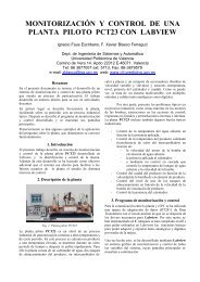
A CLOSED-LOOP TEMPERATURE CONTROL SYSTEMBY UTILIZING A LABVIEW CUSTOME-DESIGN PIDCONTROLLERMOHAMMAD A.K. ALIA, MOHAMMAD K. ABU ZALATAFaculty of Engineering TechnologyAl-Balqa’ Applied UniversityAmman, Jordonmohammed_abudaih@yahoo.comAbstract By using LabVIEW (G language), a PID control algorithm was simulated. The designed virtualinstrument includes all the necessary components and facilities necessary to function properly and to controlany linear process. The issues of integral windup, derivative overrun, output signal limits and sampling interval∆t were treated. The created Sub VI was used as a controller in a closed loop which controls an oventemperature. Results of experiment show a high degree of convergence with the results obtained when anelectronic hard-wired controller was utilized.Keywords PID algorithm, Sampling period, Integral windup, Soft-ware PID controller, Hard-wired controller.INTRODUCTIONDuring the period from the mid-fifties to the midseventies,the analog computer was widely used toobtain the response of control systems. During thattime digital computing was very costly and slowcompared to the situation today. There was littlesoft-ware available, and one had to program thesolution to a problem using machine code. Duringthe last (15) years, the picture has been drasticallychanging for the welfare of digital computers. As thecost of digital computing decreased and its speed ofoperation increased, the analog computer wasgradually replaced by the digital computer.Nowadays, to study the effect of control strategiesand controller parameters on the response of acomplex control system, one must use a computersimulation. One of the generic control strategies isthe PID control algorithm. If PID controller isproperly tuned, it will produce an acceptable controlfor most industrial processes. The PID controllerrepresents the ultimate in control of a continuousprocess for which a specific mathematicaldescription (transfer function) cannot be written[Curtis D. Johnson 1984].To program the PID algorithm using a higher-levellanguage, such as C, Pascal, or Fortran, the workwill be much easier and less error prone than whenusing assembly language. High level languagesallow us to use floating-point math. Negativenumbers and overflows are handled automatically [J.Michael Jacob, 1989]. An excellent representative ofhigh level languages is LabVIEW. Merits of thislanguage are given in detail in [NationalInstruments, 1996], [National Instruments, 2002],[Barry E. Paton 1999 ]. We think that the majoradvantage of LabVIEW over conventional high levellanguages is the graphical user interface, which isbuilt in, intuitive in operation, and simple to apply.According to [National Instruments, 2002]productivity is better with LabVIEW than withconventional languages for a factor of (5-10) timescompared with C on a small project.If one does not have PID simulation software, as inour case, it is necessary to write one's own computerprogram. It is still instructive to learn how to writecomputer programs (Virtual instruments- VIs) forthe purpose of understanding the problems andlimitations associated with commercially availablesimulation software. Examples of such problems areselecting the step size of the independent variable(∆t) or establishing initial conditions [Donald R.Coughanowr,19917]. In his valuable resource[National Instruments, 2002], Gary W. Johnsonwrites:"I wrote the PID VIs in the LabVIEW PIDcontrol Toolkit with the goal that they should beeasy to apply and modify. Every control engineerhas personal preferences as to which flavor of PIDalgorithm should be used in any particular situation.You can rewrite the supplied PID functions toincorporate your favorite algorithm. Just because Iprogrammed this particular set (which I personallytrust) doesn't mean it's always the best for everyapplication".Building on the above, we were enthusiasticallyencouraged to try to simulate the PID algorithm inour own way by using the basic LabVIEWfunctions, and to verify the simulated algorithm bytesting it practically in a temperature control system.Experimental results show that when the designedPID software and when an electronic hard-wiredPID controller were used the responses of

temperature control system for a unit-step input, arepractically the same.Another advantage of computer-based soft-warecontrol is the flexibility available in modifyingcontrol strategy. This makes it possible to do furtherimprovements to achieve better system performance.For example, it is not difficult to modify the PIDcontrol algorithm by changing the gain during thetransient period in order to minimize systemovershoot and response time, keeping at the sametime a zero steady-state offset. Hereinafter, we shalldescribe the control algorithm and illustrate theexperimental results.Programming PID AlgorithmFigure (2) Trapezoidal Method of Integrationwhere K=0, 1, 2, … n, and T = ∆t = samplingrate.The block diagram of the integral VI is shownin Figure (3).The PID controller VI consists of four Sub VIs:proportional, integral, derivative and ∆t Sub VIs.The mathematical algorithm of PID controller is asfollows:de(t)( t)= Kpe(t)+ KI ∫ e(t)dt + Kddt(1)where e(t) is the error. K p , K I , K d are coefficients ofproportional, integral, and derivative actionsrespectively.νoutProportional VIFor proportional controller only, the followingequation applies:P = K p e(t) (2)In order to get the proportional action simplymultiply the error e(t) by the constant ofproportionality (gain) K p . the block diagram isshown in Figure (1).Integral VIThe integral action is evaluated by using thetrapezoidal method. The mathematicalrepresentation of the integral action is as follows,(Figure (2)).nn ⎛ e(KT ) + e[( K + 1).T ] ⎞∫ e( t).dt = ∑ ⎜⎟.T0K = 0 ⎝ 2 ⎠(3)Figure (3) Block Diagram of IntegralAction VI.When the integral action VI is called, the while loopexecutes once because the conditional terminal isconnected to a Boolean constant (false). The errorpasses through the error control. The error value isadded to the value of the error from the pastiteration. This is done by the shift register. Then thevalue of the summation is divided by 2 andmultiplied by the gain K I and the sample time ∆t.After that, a Boolean value passes through theBoolean control PID in range?. This is toinvestigate whether the PID output limits arereached or not. If the Boolean value is true, thismeans that the PID output lies within its limits, andthe calculated value of integration is added to theprevious values. If the Boolean value is false thenthe PID is saturated and the value at the output ofthe integral action must stay constant until the PIDoutput is within the range again.Derivative VIFigure (1) Block Diagram ofProportional Action VIThe mathematical equation of the derivative actionis the following:de(t)ν o . d= K d(4)dtThe derivative action will be calculated by using thebackward difference method, Figure (4):

de(t)e(KT) − e[(K −1).T]=dtTsubtracted from this value. The result is the time inmillisecond elapsed between the first call and thesecond call of this VI. After dividing this value by1000, the result is in seconds.Figure (4) Backward Difference MethodThe block diagram of derivative VI is shown inFigure (5). The process variable passes to the VIthrough the P v control. The past value of the processvariable is subtracted from the current P v value, thenthe result is divided by the sample time ∆t, and thefinal result, after division, is multiplied with thederivative gain (K d ). Using the select function, acondition to prevent the division by zero (in casethat ∆t was zero) is included. If ∆t is larger thanzero, the calculated value passes out to theDerivative action indicator. If ∆t is less or equal tozero, for some reasons, then a value of zero is passedto the Derivative action indicator.Figure (5) Block Diagram of Derivative VI.∆t Virtual InstrumentThis VI is necessary to calculate the time periodbetween every two samples (∆t). This VI is veryimportant because it is needed for real time control.It has only one output and has no input. The blockdiagram is shown in Figure (6). The tick countfunction returns the internal timer of the CPU inmilliseconds. The reference time isundefined, so the tick count value cannot beconverted to real world time. The timer value warpsform (2 32 -l) to zero. In the first iteration of the loopthe tick count function gives the internal timer value,then the initial value stored in the shift register(which is equal to zero in the first iteration) isFigure (6) Block Diagram of ∆t VIIn the first call for this VI, the time differencebetween the first iteration and the previous one is theinternal timer value. Because this value is notreferenced to a known value, it is very large and isnot a true time value, so, it must not be passed out.For this purpose a condition statement wasdeveloped by comparing this value to an arbitrarynumber which represents the maximum delayallowed. If this value is larger than the arbitrarynumber, then it passes a number 0.01, that is close tothe real value in the following iterations. If the valueis smaller than this arbitrary number, then the VIpasses the value, which is the right time difference.In the next iteration, the value of the tick count givesthe present internal timer value. By subtracting theprevious value stored in the shift register from thepresent value of the tick count, we get the timeelapsed between this iteration and the past iteration,which is the time needed to execute the wholeprogram once. In other words, it is the time betweenthe first sample and the next sample.Complete PID VIThe PID output is the sum of the outputs of theproportional, integral and derivative actions. Thefront panel and block diagram of the PID VI areshown in Figure (7). The values of process variable(P v ) and the error e(t) are passed to the PID VIthrough the P v and error controls. The output of thePID passes out through the PID output indicator.If the output of the PID is within the range betweenupper limit and lower limit controls, then this valuepasses out at Coerced(x) terminal and a trueBoolean value at In Range? terminal of the InRange and Coerce function. If the output of thePID VI is larger than the upper limit, then the valueof the upper limit passes out and False passes to theshift register. But if the output of the PID VI is lessthan the lower limit, the value of the lower limitpasses out and False value passes to shift register.

Here, the Boolean value is used to prevent theintegral wind up.electronic PID controller. The principal circuit of theexperiment board is given in Figure (8). The frontpanel and the block diagram of the temperaturecontrol VI are shown in Figure (9).(a)Figure (9)a- Temperature Control VI FrontPanel(b)Figure (7) a- PID VI Front Panelb- PID VI Block DiagramTemperature Control by Using PID VirtualInstrumentThe temperature control system is a laboratoryexperiment board manufactured by DELLRENZO-Italy [Gary W.Johnson 1994](b)(c)Figure (9)b-Temperature Control VI Block Diagramc- Sequence 1Results of ExperimentsFigure (8) RGT1 BoardThe board allows to experimentally investigate boththe temperature measurements and closed looptemperature control. The board includes an electricoven model, temperature transducers and anelectronic hard-wired PID controller. Forcomparison purposes, oven temperature wascontrolled by the simulated PID (VI) and the built in1- Proportional Only Control Mode by Using PIDVI. Figure (10) shows system response for threedifferent values of system gain. By increasing thegain the offset decreases, and the time rise decreasesalso.

2- P, PI, and PID Control, When Using PIDVI.Figure (11) shows system responses for the threemodes of control.3- System Responses, When It Was Exited fromthe Load-Side, and by Changing the Setpoint,(input side)System responses are shown inFigure (12)4- Comparison Between the Hard-Ware and Soft-Ware Controlled System.Figure (13) illustrates the achieved responses forP, PI, modes of control.CONCLUSIONS1. By using basic LabVIEW controls, indicators andblock diagram functions, a graphical PID controllerwas designed and tested.(b)Figure (12)a- System Response to Load Disturbanceb- System Response to Change in Set Point(a)Figure (10) Proportional Control whereK p = 2, 8, and 35(b)Figure (11) System Response to P, PI, PIDControllers.Figure (13): a- Response to Hardware andSoftware P Controller; b- Response to Hardwareand Software PI ControllerCreating a Sub VI which resembles the builtelectronic controller makes it easier to tune thecontroller through variation of the controls K p , K I ,and K d , without referring to the internal componentsof the PID block diagram.(a)2.By using the front panel, simulation of the PIDalgorithm gives the user flexibility to observe in realtime the variation of any input, output andintermediate system variable, and to carry out onlineexcitation from the load side or from the inputside.

3.When realizing software PID controller, it is easyto include the necessary additional modificationsand enhancements such as integral windup,derivative overrun, controller output limits, andselection of the sampling interval4.Experimental results show that there is a highdegree of convergence between the performance ofthe software PID controller and the performance ofthe electronic hard-wired PID controller, when bothwere utilized in closed-loop temperature control.REFERENCESBarry E. Paton 1999,” LabVIEW GraphicalProgramming for Instrumentation”. Prentice HallPTP, New Jersey , U.S.ACurtis D. Johnson 1984,” Microprocessor-BasedProcess Control”. Prentice-Hall International, IncEnglewood Cliffs, NJ , U.S.A.DE-LORENZO, 2002 ,Electronic Laboratory,”(Basic Board To Study Temperature Regulation)”.DL.2155RGT1, Dl.2155RGT2, Milano, ItalyDonald R. Coughanowr,1991,”Process SystemsAnalysis and Control”. McGraw-Hill, Inc.,SingaporeGary W. Johnson, 1994. “LabVIEW GraphicalProgramming”. McGraw-Hill, Inc., New york,U.S.AJ. Michael Jacob, 1989,” Industrial ControlElectronics”. Prentice-Hall International, Inc., NewJersey , U.S.ANational Instruments, 2002, LabVIEW BasicsIntroduction, Course Manual, U.S.ANational Instruments, 1996, “LabVIEW GraphicalProgramming for Instrumentation”. User Manual.New Jersey , U.S.A