3. COMPLEX CONTROL SYSTEMS

4. Complex Control Systems 5supply chilled water to many AHUs. Therefore, flow rate change in one AHU branch will affectall other loops. When conventional single loop temperature control scheme is used with theoutput of the temperature controller applied directly to the control valve, no correction will bemade until its effect reaches the temperature measuring elements. Thus, there is a considerablelag in correcting flow rate disturbances.To improve the response of the simple feedback control to changes in chilled water supplypressure, the pressure drop across the control valve is measured to adjust the valve positionbefore the cooling exchanger reacting mixture has felt its effect. Thus, if pressure goes up,decrease the valve opening of the chilled water to keep constant chilled water supply, and viceversa. With a cascade control technique using a separate flow rate control loop, the flow ratecontroller will correct any change in the chilled water flow rate. Fig. shows a schematic diagramof the cascade control system for supply air temperatureExhust airReturn airExhust fanDampMACooling coilSupply fanFresh airSupply airTCFCFTChilled waterTTMA= mixed airTT=temperature transmitterTC=temperature controllerFT=flow transmitterFC=flow controllerBasic Principles of Cascade ControlGeneral structure of block diagram of cascade controlKNU/EECS/ELEC835001Dr. Kalyana Veluvolu

Inspection on receiptInspection on receiptFault free and safe use of this device requiresappropriate transport, proper storage, erectionand assembly as well as careful operation andmaintenance. If it can be assumed that safeoperation is no longer possible, the devicemust be immediately taken out of service andsecured against being accidentally startedup.The device must be unpacked and packedwith the usual care, without the use of forceand only using suitable tools. The devicesmust be visually inspected for perfectmechanical condition. Please also note andfollow the installation instructions enclosedwith the device.It can be assumed that safe operation is nolonger possible if the device, e.g.• has visible damage,• no longer works, despite intact mains powersupply,• has been exposed to unfavourable conditions(e.g. storage outside the permissible climaticlimits without adjustment to the ambientclimate, condensation, or similar) for a lengthyperiod or was exposed to unfavourable effectsor loads during transport (e.g. fall from a largeheight even if there is no visible externaldamage, or similar).Please check the scope of supply forcompleteness before you start installing thedevice.mmmAll screw-type terminals belonging tothe scope of supply are plugged intothe device.The installation and start-up instructionsalso describe options which donot belong to the scope of supply.All supplied options and designversions are described on the deliverynote.6

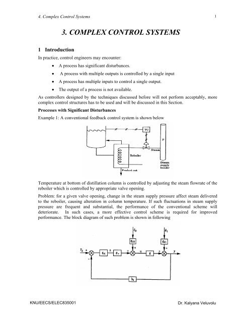
4. Complex Control Systems 9Conventional feedback control suffers from frequent disturbances in feed temperature, and thecontroller must wait until these have upset the process before feedback action can be taken.Cascade control is not a solution, as the disturbance is not associated with the manipulatedvariable.However, if we measure the feed temperature T i , then configure a feedforward controller shownas following. The feedforward controller then makes adjustments in the steam flowrate to theheating coil in response to observed changes in T i .The difference between feedforward and conventional feedback controls:• Feedforward control: compensation for the effect of a measured disturbance is possiblebefore the process is affected• Conventional feedback control: corrective action can only be taken after the process hasregistered the effect of the disturbance.Perfect disturbance rejection – not possible with feedback control-is possible (theoretically) withfeedforward control.The process output is never measured in feedforward control.Design of Feedforward ControllersConsider the following general transfer function model for a process relating manipulatedvariable and disturbance to process output, with no controller yet attached:y( s)= g ( s)u(s)+ g ( s)d ( s)The objective is for y(s) to equal its set-point value, y d (s), at all times, regardless of changes ind(s).dKNU/EECS/ELEC835001Dr. Kalyana Veluvolu

4. Complex Control Systems 10Derive the u(s) required to make y(s) = y d (s) for all time.This translates to the problem of solving the above equation for u upon setting y = y d ; doing thisgives:org st (s) is the set-point tracking controller;g ff (s) is the disturbance rejection controller.1 g ( s)u( s)= y d(s)g(s)− ddg(s)u( s)= g ( s)y g ( s)d(s)st d+ffThe block diagram of the feedforward control system is shown in the followingNote:1. The scheme can, in principle, be used both for set-point tracking (the servo problem), anddisturbance rejection (the regulatory problem). Observe that for servo problems (d =0),the controller equation is:u ( s)= g ( s)for the regulator problem (y d = 0), we have:sty du( s)= g ( s)d(s)ffHowever, it is almost exclusively associated with disturbance rejection; it is hardly everused for set-point tracking.2. In both set-point tracking and disturbance rejection, the controller has no access tomeasurements of y, it is focused on the potential cause of the upset (changes in y d or d). Itrelies on the accuracy of the process transfer function models to ensure that the desiredbehavior is obtained, even though y itself is not monitored.The feedforward control is possible when:• The disturbance d is measured, and• The effect of d on the output y is available.Example: DESIGN OF A FEEDFORWARD CONTROLLER FOR STIRRED MIXING TANK.KNU/EECS/ELEC835001Dr. Kalyana Veluvolu

4. Complex Control Systems 11The first task is to monitor the inlet temperature T i , so as to have a measurement of thedisturbance d.Its transfer function model is given as:g ( s )g d( s )where the parameters β and θ are given by==⎛⎜⎝βθ1 + θ s⎛⎜⎝Vθ = andF⎞⎟⎠11 + θ s⎞⎟⎠λβ =ρVC Prespectively, where V: tank volume, ρ: liquid density, C p : specific heat capacity, λ: latent heat ofvaporization of steam, F: volumetric flowrate.Solution: According to the design procedure given above, the equation for the feedforwardcontroller therefore is:1+θs1u( s)= yd− d(s)βθ βθNow, we investigate the controller performance and the overall behavior of the stirred mixingtank system in response to a step change of magnitude A in the set-point y dThe feedfdrward controller equation for set-point tracking is:su(s)= 1 + θβθand since, in this case, y d (s) = A/s, we have:The overall system response is now obtained:which gives:y dA Au ( s)= +βθsββθy( s)= u(s)1+θsKNU/EECS/ELEC835001Dr. Kalyana Veluvolu

4. Complex Control Systems 12resultwhich, when inverted back to time, givesA ⎛ 1 ⎞y(s)= ⎜ + θ ⎟1+θs⎝ s ⎠y ( s)=Asy ( t)= AThe implication of this result is that the system output, y(t), tracks the desired set-point perfectly.It means; so long as the process model matches the actual process behavior, this feedforwardscheme always gives the result that y = y d for all time regardless of the particular form of y d .In practice, the process model will typically not match the process behavior exactly and suchperfect set-point tracking will no longer be possible and steady-state offsets will be inevitable.Disturbance rejection: The feedforward controller equation for disturbance rejection is:inverted back to time gives:Substitute β and θ into u(t)1u( s)= − d(s)βθ1u( t)= − d ( t)βθFρCpu( t)= − d(t)λIf d(t) increases from its initial value of 0 to a new value δ (i.e., T i increases from T is to T is + δ);thenFρCu(t)= −pδλcontrol action calls for the energy input to the process to be reduced by that factor.As FρC p δ is the amount of additional energy brought into the system as a result of the increasein T i , the control is an exact counterbalancing of the disturbance effect.The tank temperature is unaffected by whatever fluctuations the inlet stream temperature T i mayexperience, result a situation of perfect disturbance rejection.Practical ConsiderationsThe system suffers from some significant drawbacks:1. It is not useful if d cannot be measured;2. Even when d is measurable, the scheme requires a perfect process model to achieve itsobjectives;KNU/EECS/ELEC835001Dr. Kalyana Veluvolu

4. Complex Control Systems 133. Even a perfect process model exists, the derived feedforward controller transfer functions -both g st and g ff involve the reciprocal of the process transfer function g as1 gd( s)u( s)= yd − d(s)g(s)g(s)may therefore present any of the following problems:(a) They may be too complicated to be realizable in time.(b) If g has a time delay element e -αs then its reciprocal will contain the term e αs ,implying that implementing g st in real time will require a prediction.(c) If both g and g d have time-delay elements, and the time delay associated with g d isless than that associated with g, then g ff will contain a term in e γs where γ > 0; again,prediction is required to implement such a controller in real time.Under the conditions specified in (b) and (c), the controllers are said to be physicallyunrealizable since, at time t, each of these controllers will require knowledge of the value thaty d (t), or d(t) will take at some time in the future; in (b) y d (t + α) is required, in (c), d(t +γ) isrequired. It is, of course, impossible to predict these quantities exactly.Feedforward control has proved to be a very powerful process control scheme, especially fordisturbance rejection.(1) Many process disturbances are indeed measurable;(2) Even when the available process models are imperfect and/or the derived g ff is toocomplicated, the lead/lag unit provides reasonably good performance as a feedforwardcontroller.Application of Lead/Lag Units in Feedforward ControlRecall the Cohen and Coon process reaction curve technique for approximate process dynamiccharacterization, in which a general approximate representation for many g and g d elements is:andg−αsKeg(s)=1+τsd( s)=Kde−βs1+τ sleading to a g ff having the following generalized form:This simplifies to:ggffff−βsKde1+τs( s)= −−αs1+τ s Kedd( 1+τs) −γsKff( s)= −1+τ swhich is a lead/lag unit with a time delay. In the event that α and β are approximately equal, theabove Eq. is a pure lead/lag element.deKNU/EECS/ELEC835001Dr. Kalyana Veluvolu

4. Complex Control Systems 14This offers an objective justification for the effectiveness of lead/lag units in the implementationof feedforward control schemes even in situations when the dynamic behavior of the processes inquestion is poorly modeled.Tuning the Lead/Lag Unit1. Obtain approximate characterizing process parameters Obtain process reaction curves for(a) The response of the process output to a step change in the input U (with d =0), and(b) The corresponding process response to a step change in the disturbance d (with U = 0).Characterize each response by their respective steady-state gains, and effective timeconstants, and time delays as given in above equations.2. Estimate lead/lag unit parametersFrom the six parameters obtained from the two process reaction curves, we obtain thelead/lag unit parameters as follows:Gain term: K ff =K d /KLead time constant:τLag time constant: :τ dAssociated delay: γ=β−α4. Feedback/Feedforward ControlWeaknesses of feedforward control:1. Identification of all disturbances and their direct measurement, not possible for manyprocesses.2. Any changes in the parameters can not be compensated, because they can not bedetected.3. Requires a good model for the process, not possible for many systems.Feedback control is insensitive to all three of these drawbacks but has other drawbacks:FeedbackFeedforwardNot require identification and measurement ofdisturbanceInsensitive to modeling errors.Insensitive to parameter changes.Control action is taken after disturbances havebeen felt.Unsatisfactory for slow and significant dead timeprocess.It may create instability in the closed-loopresponse.AdvantagesActs before a disturbance has been felt by the system.Good for slow systems or significant dead time.Not introduce instability in the closed-loop response.DisadvantagesRequires all disturbances and their direct measurement.Cannot cope with unmeasured disturbances.Sensitive to process parameter variations.KNU/EECS/ELEC835001Dr. Kalyana Veluvolu

4. Complex Control Systems 16gd( s)gff( s)= −g(s)the effect of d on y is theoretically eliminated.Important points about the feedforward/feedback scheme:1. The overall system stability is determined by the roots of the closed-loop system’scharacteristic equation:1 + gg ch = 0Observe that this has nothing to do with g ff . The stability of the feedback loop remainsunaltered by including feedforward compensation. This is a very significant point infavor of the feedforward control scheme; in terms of closed loop stability, we havenothing to lose by applying it.2. When g d and g are perfectly known, perfect compensation is possible; in the morerealistic case where this is not the case, and/or the disturbances are (partially orcompletely) unmeasurable, the feedback loop picks up the residual error and eliminatesit with time.5 Ratio ControlIn certain situations, the value observed for d is to be a certain percentage of another processinput variable.In this case, the objective is to maintain a constant ratio between d and this other variable. Thusas d changes, this other variable also changes in order to maintain the desired ratio.The control scheme is called ratio control; it is a special form of feedforward control.Process Flow ApplicationsRatio control mostly applied in systems that involve mixing of two or more process streams. Insuch process flow applications, there are typically two streams whose flowrates are to bemaintained at a certain prespecified proportion.Both flowrates are measurable, usually the flowrate of one stream can be controlled while theother flowrate cannot be controlled but can be measured.The stream whose flowrate cannot be controlled is referred as: wild stream.Consider the process as shown in the Figure, a salt solution mixer for which the salt concentrateflowrate can be regulated but the water flowrate cannot. It makes the water stream the "wildstream."To maintain uniform salt concentration within the mixing tank, it is necessary to maintain aconstant ratio of water and salt concentrate flowrates.A ratio control scheme to achieve this objective can be set up in one of the two ways shown inthe following FiguresKNU/EECS/ELEC835001Dr. Kalyana Veluvolu

4. Complex Control Systems 17Under the strategy indicated in Figure (a),• Both flowrates are measured and their current ratio obtained by an electronic divider.• The observed ratio is transmitted to the ratio controller where it is compared to the desiredratio set-point; the error is used to set the flowrate required for the salt concentrate stream.The actual current ratio of the flowstreams is the information obtained from the process andpassed on to the controller; the controller will now have to use this information to calculate, andKNU/EECS/ELEC835001Dr. Kalyana Veluvolu

4. Complex Control Systems 18implement the change needed in the salt concentrate flowrate to attain to the desired ratio.Another strategy indicated in Figure (b)• The "wild stream" flowrate is measured and multiplied at the "ratio station" by the desiredratio; this produces the value of the flowrate at which the other stream must be set tomaintain the desired ratio.• The output of the ratio station is the set-point for the flow controller; it is compared with theactual flowrate of the salt concentrate stream, and the controller acts on the basis of theobserved deviation.In this case there is a flow controller that directly regulates the flowrate of the salt concentratestream; the information it receives from the ratio station is its set-point.Two Loops Ratio ControlIn the case it requires high control quality and no wild stream, It is nature to control both loops.KNU/EECS/ELEC835001Dr. Kalyana Veluvolu

4. Complex Control Systems 20Problem: The outside metal surface temperature of the tubes containing the crude oil mustremain below the metallurgical limit of the tube material.Override controllers can be used to maintain the tube surface temperature below this criticalvalue. The override control scheme is shown in the followingThe optical pyrometers are used to measure the tube surface temperature at several locationsalong the tube.One of these tube temperature measurements are selected and send it to a temperature controllerand High Selector (HS) switch. When the measured tube temperature exceeds a preset criticalvalue, the HS switches from the "normal" loop to the "abnormal" loop in which the fuel flowrateis adjusted to control tube skin temperature at a preset safe maximum.When the "normal" loop calls for less fuel than required to maintain the maximum tube surfacetemperature, the selector will switch back to the "normal" loop.In this way the crude oil exit temperature from the furnace will be maintained at its set-pointexcept when the tube surface temperature is exceeded.During "abnormal" operation, the crude oil exit temperature will be somewhat below its setpoint,but as close as possible while ensuring safe operation of the furnace.Example 2: Protection of a boiler system:1. The steam pressure in a boiler is controlled through the use of a pressure control loop on thedischarge.2. Water level in the boiler should not fall below a lower limit which is necessary to keep theheating coil immersed in water and thus prevent its burning out.Figure shows the override control system using a low switch selector (LSS). Whenever the liquidlevel falls below the allowable limit, the LSS switches the control action from pressure control tolevel control (loop 2 in the Figure) and closes the valve on the discharge line.KNU/EECS/ELEC835001Dr. Kalyana Veluvolu

4. Complex Control Systems 21Auctioneering ControlA second type of selective control is so-called "auctioneering" control. This is where there is afixed control loop, but the output variable to be used may change. This may be illustrated by thefurnace example of the previous section.The tube surface temperature was measured at several locations, for the "abnormal" loop we areinterested in the location with the highest tube surface temperature. A HS switch is added tochoose the highest temperature of those measured in regulating the tube surface temperature. Itensures that the highest measured temperature is maintained at a safe level.Example: Several highly exothermic reactions take place in tubular reactors filled with a catalystbed.The Figure shows the temperature profile along the length of the tubular reactor.Hot spot: The point of highest temperature along the length of the tubular reactor.KNU/EECS/ELEC835001Dr. Kalyana Veluvolu

4. Complex Control Systems 22Variation Factors:• Feed conditions (temperature, flow rate, concentration)• Catalyst activity• Temperature and flow rate of the coolant.7 Multiple Inputs Control Single OutputIn this configuration, there are two or more manipulated variables available for the control of asingle-output variable.Split-Range ControlSplit-range control is the usual solution when one requires multiple manipulated variables inorder to span the range of possible set-points.Example: Suppose there is a nonisothermal batch reactor with a certain specified temperatureprogram required to produce the product.• The temperature ranging from 15 0 C at the beginning of the batch to 100 0 C at the end.• The cooling water is at 5 0 CKNU/EECS/ELEC835001Dr. Kalyana Veluvolu

4. Complex Control Systems 23• The low-pressure steam is at 180 0 C.It requires both cooling water and steam in order to span the temperature range of interest.Split-range control allows both cooling water and steam to be used as shown in the Figure:Note that the schedule allows the appropriate fraction of cooling water and steam to be used foreach value of the controller output signal and reactor jacket inlet temperature required. Usuallythe design uses overlap in the range of each valve for more precise control.Split-range control is often employed for broad span temperature control of small plant, and foryear-round heating and cooling of office buildings.Multiple Inputs improving DynamicsMultiple inputs are also employed in order to speed up the dynamic response of a process duringserious upsets or transitions between set-points.Example: Consider the stirred heating tank, but now assume that there is an additional auxiliaryelectrical heater and cooler that can be used to control the tank temperature as shown in theFigure:The heating tank has several temperature set-points depending on the product being made in adownstream reactor. The normal regulatory operation at each of these set-points can be readilyKNU/EECS/ELEC835001Dr. Kalyana Veluvolu

4. Complex Control Systems 24handled with the process steam going to the tank heating coil.It is important for the downstream reactor that set-point changes be made rapidly but the stirredheating tank temperature responds rather slowly even with the steam valve full open or full shut.Thus for an increase in temperature set-point the auxiliary heater helps speed the move to thenew set-point. Similarly when the temperature set-point change is down, the auxiliary coolerhelps the tank quickly achieve the new set-point.The drawback is that this auxiliary heater and cooler require expensive electrical energy whilethe steam to the coil is very cheap because it is produced as a byproduct from another processunit. Thus, the auxiliary heater and cooler be used only during set-point changes.This could be accomplished with three controllers as shown in Figure above with a scheduledefining when each controller is active. For example, one could choose the following schedule toachieve the control objective.CONTROLLER SCHEDULEDeviation from set-pointController active∆T < - 10 0 CTC3+TC1- 10 0 C < ∆T < + 10 0 C TC1∆T > + 10 0 CTC2+TC1The controllers TC2 and TC3 could be on-off controllers or proportional controllers withsuitable gain. The controller for the steam coil would have to have integral action and be tuned toreject disturbances.8 Inferential controlGeneric problemThere exist a number of processes in which the primary variable to be controlled is difficult tomeasure or is a sampled measurement with a long delay in the sampling and analysis process.Sometimes the quantity to be controlled is a calculated variable. In such cases, control of theprocess is usually accomplished by measuring secondary variables (for which sensors are morereliable, cheaper or more readily available and installed) and setting up a feedback controlsystem using these secondary variables. Such control strategies are referred to as inferentialcontrol, the control scheme can be used when:1. Measurement of the true controlled variable is not available in a timely manner because• An on-stream sensor is not possible.• An on-stream sensor is too costly.• Sensor has unfavorable dynamics (e.g., long dead time or analysis time) or islocated far downstream.2. A measured inferential variable is available.Example 1: In distillation the primary variables to be regulated are the product compositions(bottoms and distillate purity) as shown in Figure below. Gas chromatographs typically used tomeasure these are very expensive, difficult to maintain/calibrate and introduce significantKNU/EECS/ELEC835001Dr. Kalyana Veluvolu

4. Complex Control Systems 25measurement delays because of the time needed to purge the sample line and to heat the sample.In this case, control is accomplished using temperature measurements on the intermediate trays.Example 2: In polymerization reactors, primary variables of interest are the molecular weightand viscosity of the product, as shown in Figure below. Control is accomplished usingsecondary measurements such as temperature and pressure in the reactor. The Low DensityPolyEthylene (LDPE) can be detected from online measurements such as the temperature profiledown the reactor and the solvent flow rate, which are available on a more frequent rate thanfundamental polymer properties. The estimation of polymer viscosity in a polymerizationreactor using viscometer is subject to a significant time delay but the torque from a variablespeed drive provides an instantaneous indication of reactor viscosity.Example 3: Figure below shows a third application of inferential control. This pertains to controlof industrial drying processes. The control of such drying processes is to determine solidsmoisture, a variable not usually measurable, and using this to manipulate the temperature ofdrying air until the desired target in solids moisture is obtained.KNU/EECS/ELEC835001Dr. Kalyana Veluvolu

4. Complex Control Systems 26Figure below shows the schematic of the generic problem tackled by inferential control. Thecontrol objective typically is to keep the primary variable on target in presence of unmeasureddisturbances. We first look at some classical techniques used, which while being simple toimplement can be costly because of poor controller performance.Generic inferential control problemFor the simple case of a linear system with a single disturbance, single primary output and singlesecondary measurement as in the Figure, the process can be modeled as:ys () = g ()() sus+g () sds () Primary outputuydyzs ( ) = g ( sus ) ( ) + g ( sds ) ( ) Secondary measurementsuzdz(1)Block diagram of a process with one primary and one secondary measurementKNU/EECS/ELEC835001Dr. Kalyana Veluvolu

4. Complex Control Systems 27Classical ControlConsider direct feedback control of the secondary measurement z using the manipulated variableu as shown in Figure. This strategy can be used if the primary variable and secondary variableare very closely related. For example in distillation, it is well known that temperature is a verygood indicator of product composition. Hence, by maintaining one of the tray temperaturesconstant, we can often maintain good control of the product quality.A classical approach control secondary variableTaking setpoint of z to be zero without loss of generality, the transfer function for disturbancerejection under perfect control of z can be derived as:⎛ guy() s gdz() s ⎞ys () = ⎜− + gdy() s⎟ds()⎝ guz() s⎠Note that y(s)=0 if gdz ≈ gdy and guz ≈ guy, i.e. when the disturbance d and manipulated variableu affect both z and y in a similar manner. If this is not so (which is often the case) this strategymay result in poor control.Cascade ControlIn the cascade control strategy, shown in Figure, the inner loop tries to maintain the secondaryvariable at a set point which is adjusted by the outer loop to bring y back to its set point. Thisstrategy is usually employed when there are significant delays and lags associated withmeasurement of y. To implement this strategy, we must have a measurement of the primaryvariable. The disturbance rejection transfer function is given by:whereys ()g sg() s g () suy 1 dyds ()= + (3)gcz gcygdy + gcz gdzg1=− (4)1 + g g g + g gcz cy uy cz uzKNU/EECS/ELEC835001Dr. Kalyana Veluvolu

4. Complex Control Systems 28Structure of the cascade control systemThis strategy has the advantage that steady state error in control of y will be reduced to zero ifwe use integral action in the outer loop controller. But whether this strategy will work well in aprocess depends on a number of factors. The inner loop should be able to react fast enough tofollow frequent set-point changes. If there are significant lags in the inner loop then the systemwill not have enough time to settle down, and control system performance will be poor. If thedisturbances come in at a low frequency such that the outer loop has enough time to correct it.this structure might be acceptable. However if the disturbances come at a frequency that keepsthe system from settling down then the controller on the outer loop will not have time to settledown. Because of the large delays involved in the measurement this will usually mean poorperformance of the control system.More importantly, both of the above strategies have no easy extension to the case of multiplesecondary measurements. Usually multiple secondary measurements contain more informationabout the state of the system. Thus methods that use multiple measurements have an advantageover these multi-loop strategies.Estimator Based ControlIn this strategy, an estimator for the unmeasured output y is built first which is then used in afeedback control mode. Figure 5 shows the structure and block diagram of this control strategy.Structure of the controller using state estimatorThe disturbance rejection transfer function is given byys () gdy() s=ds () 1 + g () sg () suycyNote that this is the same as what we get if we had direct feedback control on the primarymeasurement itself. The advantage with this approach is that an estimate of the unmeasured statey is available through the secondary measurements, which is useful for the operator. If g dyand gcyhave large lags associated with them, then this can result in poor performance since theKNU/EECS/ELEC835001Dr. Kalyana Veluvolu

4. Complex Control Systems 29optimum performance achievable using direct feedback control is limited by the time lags andtime delays present in the feedback loop. This controller may be worse than direct feedbackcontrol on z in some cases if z responds faster to the disturbance and manipulated variable. Inaddition, state estimators are never perfect and introduce additional errors in the feedbackcontrol loop that necessitate de tuning the controller to some extent. The construction of stateestimators is not trivial.Inferential ControlIn the classical 2-degree of freedom IMC structure an estimate of the disturbance effect on y isfed back as shown in Figure. The question inferential control tackles is how to generated = g d()s if no measurement of y is available but only z(s) is available.ydyIn this case, we can first computed () s = g () s d() s = z() s − g ()() s u s(6)z dz uzAnd then obtain an estimate of d(s) as:dycan then be estimated as follows:[ ]d s = g s z s − g s u s(7)−1e() dz() ()uz()()[ ]d s = g s d s = g s g s z s − g s u s(8)−1ye() dy()e() dy()dz() ()uz()()Using this equation we get the structure of the inferential control system as shown in FigureThe design of the disturbance controller g ( s ) is as in IMC. The output response is given bycdys () = g ()() sus+ d()s(9)uyyKNU/EECS/ELEC835001Dr. Kalyana Veluvolu

4. Complex Control Systems 30To keep y close to the set point (= 0) we choose the controller so thatus =− g sd s(10)−1()uy()y()Using the estimate of dyin place of dywe get:( )u s =−g s g s g s z s − g s u s(11)−1 −1()uy()dy()dz() ()uz()()The controller transfer function derived above may not be realizable since we have to invert theprocess transfer function. If the process transfer functions contain RHP zeros or time delays thenwe must add a filter f(s), designed as in the IMC controller, to make the controller realizable:( )u s =−f s g s g s g s z s − g s u s(12)−1 −1() ()uy()dy()dz() ()uz()()The disturbance rejection transfer function for the control scheme is given by:ys ()gdy()1 s ( f()s )ds ()= − (13)This transfer function is very similar to a feedforward controller. If the filter transfer functionused is close to 1 then we have nearly perfect rejection of disturbances as in feed forwardcontrol. In general the filter must have lag terms to compensate for modeling errors and makethe system robust.It is important to differentiate the above structure from state estimation techniques like Kalmanfilter that uses z to predict y and then control y. If the secondary measurements respond faster tothe disturbances then one can take faster corrective action and hence get better control systemperformance by using z in an inferential structure. If the output y responds to disturbancesslower than z, then the state estimator will add additional lag in the feedback loop and hence willadversely affect the performance of the control system. Usually it is possible to identifysecondary measurements closer to the disturbance and hence in general the inferential controlstrategy is preferred.Both the inferential control scheme and the state-estimation schemes outlined above can beextended to nonlinear and multivariable situations.SummaryAn inferential variable must satisfy the following criteria:1. The inferential variable must have a good relationship to the true controlled variablefor changes in the potential manipulated variable.2. The relationship in criterion 1 must be insensitive to changes in operating conditions(i.e., unmeasured disturbances) over their expected ranges.3. Dynamics must be favorable for use in feedback control.Correction of inferential variable1. By primary controller in automated cascade design2. By plant operator manually, based on periodic information3. When inferential variable is corrected frequently, the sensor for the inferentialvariable must provide good reproducibility, not necessarily accuracyKNU/EECS/ELEC835001Dr. Kalyana Veluvolu