Pattern Classification

PatternClassificationAll materials in these slides were takenfromPattern Classification (2nd ed) by R. O.Duda, P. E. Hart and D. G. Stork, JohnWiley & Sons, 2000with the permission of the authors andthe publisher

Artificial Neural Net Models• Massive parallelism is essential for highperformance cognitive tasks (speech & imagerecognition). Humans need only a few msec. formost cognitive tasks• Design a massively parallel architecturecomposed of many simple processing elementsinterconnected to achieve certain collectivecomputational capabilities• Also known as connectionist models and paralleldistributed processing (PDP) models• Derive inspiration from “knowledge” of biologicalneural nets•

Natural Neural Net Models• Human brain consists of very large number ofneurons (between 10**10 to 10**12)• No. of interconnections per neuron is between 1Kto 10K• Total number of interconnections is about 10**14• Damage to a few neurons or synapse (links)does not appear to impair overall performancesignificantly (robustness)

Artificial Neural Net Models• Artificial Neural nets are specified by• Net topology• Node (processor) characteristics• Training/learning rules• We consider only feedforward multilayernetworks• These networks essentially implement a nonparametricnon-linear classifier

Linear Discriminant Functions• A discriminant function that is a linear combination ofinput features can be written asSign of thefunctionvalue givesthe classlabelWeightvectorBias or Thresholdweight

Introduction6• Goal: Classify objects by learning nonlinearity• There are many problems for which lineardiscriminants are not sufficient for minimum error• The central difficulty is the choice of the appropriatenonlinear functions• A “brute” approach might be to select a completebasis set such as all polynomials; such a classifierwould require too many parameters to be determinedfrom a limited number of training samplesPattern Classification, Chapter 6

7• There is no automatic method for determining thenonlinearities when no information is provided to theclassifier• In using the multilayer neural Networks or multilayerPerceptrons, the form of the nonlinearity is learned fromthe training data• Multilayer networks can, in principle, provide the optimalsolution to an arbitrary classification problem• Nothing “magical” about multilayer neural networks; theyimplement linear discriminants but in a space where theinputs have been mapped nonlinearlyPattern Classification, Chapter 6

8Feedforward Operation andClassification• A three-layer neural network consists of aninput layer, a hidden layer and an output layerinterconnected by modifiable weightsrepresented by links between layers• Multilayer neural network implements lineardiscriminants, but in a space where the inputshave been mapped nonlinearly• Figure 6.1 shows a simple three-layernetworkPattern Classification, Chapter 6

9Pattern Classification, Chapter 6

10Pattern Classification, Chapter 6

11• A single “bias unit” is connected to each unit in addition tothe input units• Net activation:netdd∑ ∑tj= xiwji+ wj0= xiwji≡ wj.x,i= 1i=0where the subscript i indexes units in the input layer, j in thehidden layer; w ji denotes the input-to-hidden layer weights atthe hidden unit j. (In neurobiology, such weights orconnections are called “synapses”)• Each hidden unit emits an output that is a nonlinear functionof its activation, that is: y j = f(net j )Pattern Classification, Chapter 6

Figure 6.1 shows a simple threshold functionf ( net ) =1 if net ≥ 0sgn( net ) ≡⎩⎨⎧− 1 if net < 0• The function f(.) is also called the activationfunction or “nonlinearity” of a unit. There aremore general activation functions withdesirables properties12• Each output unit similarly computes its netactivation based on the hidden unit signals as:netnH nH=tk ∑ yjwkj+ wk0= ∑ yjwkj= wk.y,j= 1j=0where the subscript k indexes units in the ouputlayer and n H denotes the number of hidden unitsPattern Classification, Chapter 6

13• The output units are referred as z k . An output unitcomputes the nonlinear function of its net input,emittingz k = f(net k )• In the case of c outputs (classes), we can view thenetwork as computing c discriminant functionsz k = g k (x); the input x is classified according to thelargest discriminant function g k (x) ∀ k = 1, …,c• The three-layer network with the weights listed infig. 6.1 solves the XOR problemPattern Classification, Chapter 6

• The hidden unit y 1 computes the boundary:x 1 + x 2 + 0.5 = 0≥ 0 ⇒ y 1 = +1< 0 ⇒ y 1 = -1• The hidden unit y 2 computes the boundary:x 1 + x 2 -1.5 = 0≤ 0 ⇒ y 2 = +1< 0 ⇒ y 2 = -1• Output unit emits z 1 = +1 if and only if y 1 = +1 and y 2 = +1Using the terminology of computer logic, the units arebehaving like gates, where the first hidden unit is an ORgate, the second hidden unit is an AND gate, and the outputunit implementsz k = y 1 AND NOT y 2 = (x 1 OR x 2 ) and NOT(x 1 AND x 2 ) =x 1 XOR x 2which provides the nonlinear decision of fig. 6.114Pattern Classification, Chapter 6

• General Feedforward Operation – case of c output units15gk(kn⎛ Hd⎛( x ) ≡ zk= f⎜⎜ ∑ wkjf w⎝ j 1⎜⎝∑= i=1= 1,...,c)ji• Hidden units enable us to express more complicatednonlinear functions and extend classification capability• Activation function does not have to be a sign function, itis often required to be continuous and differentiable• We can allow the activation in the output layer to bedifferent from the activation function in the hidden layer orhave different activation for each individual unit• Assume for now that all activation functions are identicalxi+wj0⎞⎟⎠ +wk0⎞⎟⎟⎠(1)Pattern Classification, Chapter 6

• Expressive Power of multi-layer Networks16Question: Can every decision boundary be implemented bya three-layer network described by equation (1)?Answer: Yes (due to A. Kolmogorov)“Any continuous function from input to output can beimplemented in a three-layer net, given sufficient number ofhidden units n H , proper nonlinearities, and weights.”Any continuous function g(x) defined on the unit cube can berepresented in the following formg(x )2n + 1= ∑j=1δj( )nΣβ ( x ) ∀x∈ I ( I = [0,1];n ≥ 2 )for properly chosen functions δ j and β ijijiPattern Classification, Chapter 6

17• Eq (8) can be expressed in neural network terminology asfollows:• Each of the (2n+1) hidden units δ j takes as input a sum of dnonlinear functions, one for each input feature x i• Each hidden unit emits a nonlinear function δ j of its totalinput• The output unit emits the sum of the contributions of thehidden unitsUnfortunately, Kolmogorov’s theorem tells us very little abouthow to find the nonlinear functions based on data; this is thecentral problem in network-based pattern recognitionAnother question: how many hidden nodes we should have?Pattern Classification, Chapter 6

18Pattern Classification, Chapter 6

19Pattern Classification, Chapter 6

Neural Network Functions20Pattern Classification, Chapter 6

Backpropagation Algorithm21• Any function from input to output can beimplemented as a three-layer neural network• These results are of greater theoretical interestthan practical, since the construction of such anetwork requires the nonlinear functions and theweight values which are unknown!Pattern Classification, Chapter 6

Network Learning22• Our goal is to learn the interconnection weights based onthe training patterns and the desired outputs• In a three-layer network, it is a straightforward matter tounderstand how the output, and thus the error, dependson the hidden-to-output layer weights• The power of backpropagation is that it enables us tocompute an effective error for each hidden unit, and thusderive a learning rule for the input-to-hidden weights. Thisis known as:The credit assignment problemPattern Classification, Chapter 6

• Network has two modes of operation:23• FeedforwardThe feedforward operations consists of presenting apattern to the input units and passing (or feeding) thesignals through the network in order to yield adecision from the outputs units• LearningThe supervised learning consists of presenting aninput pattern and modifying the network parameters(weights) to bring the actual outputs closer to thedesired target valuesPattern Classification, Chapter 6

24Pattern Classification, Chapter 6

Network Learning• Start with an untrained network, present a trainingpattern to the input layer, pass the signal through thenetwork and determine the output.• Let tk be the k-th target (or desired) output and zk bethe k-th computed output with k = 1, …, c. Let wrepresent all the weights of the network• The training error:J(w )=12c∑k = 1( tk−zk)2=12t−z225• The backpropagation learning rule is based ongradient descent• The weights are initialized with random values and arechanged in a direction that will reduce the error:∆ w= −η∂∂JwPattern Classification, Chapter 6

where η is the learning rate which indicates the relativesize of the change in weightsw(m +1) = w(m) + ∆w(m)where m is the m-th training pattern presented26• Error on the hidden–to-output weights∂J∂wkj=∂J∂netwhere the sensitivity of unit k is defined as:k∂net.∂wand describes how the overall error changes with theactivation of the unit’s net activation∂J∂J∂zkδk= − = − . = ( tk− zk) f' ( netk)∂net∂z∂netkkkjkk= −δk∂net∂wδkjkk∂J= −∂netkPattern Classification, Chapter 6

27Since net k = w kt .y, therefore:∂net∂wkjk=yjConclusion: the weight update (or learning rule) for thehidden-to-output weights is:∆w kj = ηδ k y j = η(t k – z k ) f’ (net k )y j• Learning rule for the input-to-hiden units is more subtleand is the crux of the credit assignment problem• Error on the input-to-hidden units: Using the chain rule∂J∂wji=∂J∂yj∂yj.∂netj∂net.∂wjijPattern Classification, Chapter 6

However,∂J∂yj= −∂=∂yj⎡⎢⎣12c∑k=1( tk∂z− z∂netSimilarly as in the preceding case, we define the sensitivityof a hidden unit:cAbove equation is the core of the “credit assignment”problem: “The sensitivity at a hidden unit is simply the sumof the individual sensitivities at the output units weighted bythe hidden-to-output weights w kj, all multiplied by f’(net j )”;see fig 6.5Conclusion: Learning rule for the input-to-hidden weights:= −∑k=1cckk∑( tk− zk) . = −∑k= 1 ∂netk∂yj k=1k)2⎤⎥⎦δj≡c( tk( t− zkk− zf'( net∂z)∂ykjkj) f' ( net)∑k=1kwkj)wδkjk28[ Σw]kjδkf ' ( netj) xi∆ wji= ηxiδj= η δjPattern Classification, Chapter 6

Sensitivity at Hidden Node

Backpropagation Algorithm30• More specifically, the “backpropagation oferrors” algorithm• During training, an error must be propagatedfrom the output layer back to the hidden layer tolearn the input-to-hidden weights• It is gradient descent in a layered network• Exact behavior of the learning algorithmdepends on the starting point• Start the process with random values of weights;in practice you learn many networks withdifferent initializationsPattern Classification, Chapter 6

• Training protocols:• Stochastic: patterns are chosen randomly from trainingset; network weights are updated for each pattern• Batch: Present all patterns before updating weights• On-line: present each pattern once & only once (nomemory for storing patterns)• Stochastic backpropagation algorithm:31Begin initialize n H ; w, criterion θ, η, m← 0do m ← m + 1x m ← randomly chosen patternw ji ← w ji + ηδ j x i ; w kj ← w kj + ηδ k y juntil ||∇J(w)|| < θreturn wEndPattern Classification, Chapter 6

• Stopping criterion32• The algorithm terminates when the change in thecriterion function J(w) is smaller than some presetvalue θ; other stopping criteria that lead to betterperformance than this one• A weight update may reduce the error on the singlepattern being presented but can increase the error onthe full training set• In stochastic backpropgation and batch propagation,we must make several passes through the trainingdataPattern Classification, Chapter 6

• Learning Curves33• Before training starts, the error on the training set is high;as the learning proceeds, error becomes smaller• Error per pattern depends on the amount of training dataand the expressive power (such as the number ofweights) in the network• Average error on an independent test set is always higherthan on the training set, and it can decrease as well asincrease• A validation set is used in order to decide when to stoptraining ; we do not want to overfit the network anddecrease the power of the classifier’s generalization“Stop training when the error on the validation set isminimum”Pattern Classification, Chapter 6

34Pattern Classification, Chapter 6

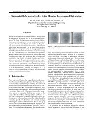
Representation at the Hidden Layer• What do the learned weights mean?• The weights connecting hidden layer to outputlayer form a linear discriminant• The weights connecting input layer to hiddenlayer represent a mapping from the inputfeature space to a latent feature space• For each hidden unit, the weights from inputlayer describe the input pattern that leads tothe maximum activation of that node

Backpropagation as Feature MappingInput layer to hidden layer weights for a character recognition taskWeights at two hidden nodesrepresented as 8x8 patternsLeft gets activated for F, right getsactivated for L, and both getactivated for E• 64-2-3 sigmoidal network for classifying three characters (E,F,L)• Non-linear interactions between the features may cause thefeatures of the pattern to not manifest in a single hidden node (incontrary to the example shown above)• It may be difficult to draw similar interpretations in large networksand caution must be exercised while analyzing weights

Practical Techniques for ImprovingBackpropagation• A naïve application of backpropagation procedures maylead to slow convergence and poor performance• Some practical suggestions; no theoretical results• Activation Function f(.)• Must be non-linear (otherwise, 3-layer network is just a lineardiscriminant) and saturate (have max and min value) to keepweights and activation functions bounded• Activation function and its derivative must be continuous andsmooth; optionally monotonic• Choice may depend on the problem. Eg. Gaussian activation ifthe data comes from a mixture of Gaussians• Eg: sigmoid (most popular), polynomial, tanh, sign function• Parameters of activation function (e.g. Sigmoid)• Centered at 0, odd function f(-net) = -f(net) (anti-symmetric);leads to faster learning• Depend on the range of the input values

Activation FunctionFirst & second derivativeThe anti-symmetric sigmoid function: f(-x) = -f(x).a = 1.716, b = 2/3.

Practical Considerations• Scaling inputs (important not just for neural networks)• Large differences in scale of different features due to the choice ofunits is compensated by normalizing them to be in the same range,[0,1] or [-1,1]; without normalization, error will hardly depend onfeature with very small values• Standardization: Shift the inputs to have zero mean and unitvariance• Target Values• One-of-C representation for the target vector (C is no. of classes).Better to use +1 and –1 that lie well within the range of sigmoidfunction saturation values (+1.716, -1.716)• Higher values (e.g. 1.716, saturation point of a sigmoid) mayrequire the weights to go to infinity to minimize the error• Training with Noise• For small training sets, it is better to add noise to the input patternsand generate new “virtual” training patterns

Practical Considerations• Number of Hidden units (n H )• Governs the expressive power of the network• The easier the task, the fewer the nodes needed• Rule of thumb: total no. of weights must be less than the number oftraining examples (preferably 10 times less); no. of hidden unitsdetermines the total no. of weights• A more principled method is to adjust the network complexity inresponse to training data; e.g. start with a “large” no. of hidden unitsand “decay”, prune, or eliminate weights• Initializing weights• We cannot initialize weights to zero, otherwise learning cannot takeplace• Choose initial weights w such that |w| < w’• w’ too small – slow learning; too large – early saturation and nolearning• w’ is chosen to be 1/√d for input layer, and 1/ √n H for hidden layer

Total no. of WeightsError per pattern with the increase in number of hidden nodes.• 2-n H -1 network (with bias) trained on 90 2D-Gaussian patterns (n =180) from each class (sampled from mixture of 3 Gaussians)• Minimum test error occurs at 17-21 weights in total (4-5 hiddennodes). This illustrates the rule of thumb that n/10 weights often giveslowest error

Practical Considerations• Learning Rate• Small learning rate: slow convergence• Large learning rate: high oscillation and slow convergence

Practical Considerations• Momentum• Prevents the algorithm from getting stuck at plateaus and localminima• Weight decay• Avoid overfitting by imposing the condition that weights must besmall• After each update, weights are decayed by some factor• Related to regularization (also used in SVM)• Hints• Additional input nodes added to NN that are onlyused during training. Help learn better featurerepresentation.

Practical Considerations44• Training setup• Online, stochastic, batch-mode• Stop training• Halt when validation error reaches (first) minimum• Number of hidden layers• More layers -> more complex• Networks with more hidden layers are more prone toget caught in local minima• Smaller the better (KISS)• Criterion function• We talked about squared error, but there are othersPattern Classification, Chapter 6