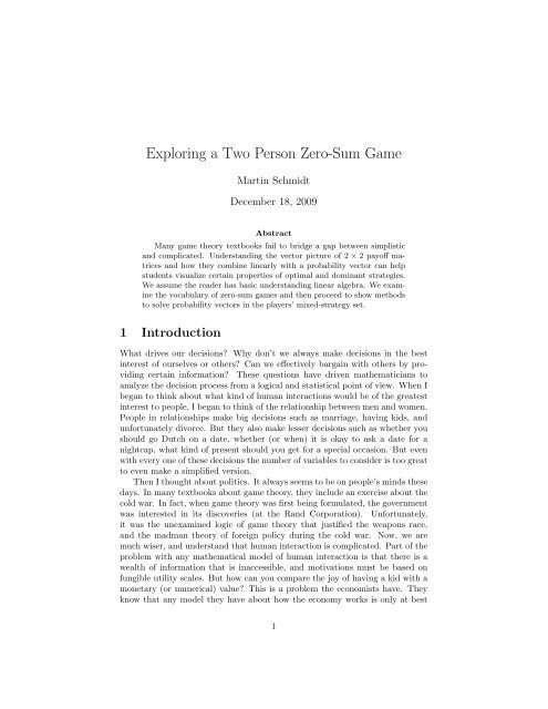
Exploring a Two Person Zero-Sum Game

Exploring a Two Person Zero-Sum GameMartin SchmidtDecember 18, 2009AbstractMany game theory textbooks fail to bridge a gap between simplisticand complicated. Understanding the vector picture of 2 × 2 payoff matricesand how they combine linearly with a probability vector can helpstudents visualize certain properties of optimal and dominant strategies.We assume the reader has basic understanding linear algebra. We examinethe vocabulary of zero-sum games and then proceed to show methodsto solve probability vectors in the players’ mixed-strategy set.1 IntroductionWhat drives our decisions? Why don’t we always make decisions in the bestinterest of ourselves or others? Can we effectively bargain with others by providingcertain information? These questions have driven mathematicians toanalyze the decision process from a logical and statistical point of view. When Ibegan to think about what kind of human interactions would be of the greatestinterest to people, I began to think of the relationship between men and women.People in relationships make big decisions such as marriage, having kids, andunfortunately divorce. But they also make lesser decisions such as whether youshould go Dutch on a date, whether (or when) it is okay to ask a date for anightcap, what kind of present should you get for a special occasion. But evenwith every one of these decisions the number of variables to consider is too greatto even make a simplified version.Then I thought about politics. It always seems to be on people’s minds thesedays. In many textbooks about game theory, they include an exercise about thecold war. In fact, when game theory was first being formulated, the governmentwas interested in its discoveries (at the Rand Corporation). Unfortunately,it was the unexamined logic of game theory that justified the weapons race,and the madman theory of foreign policy during the cold war. Now, we aremuch wiser, and understand that human interaction is complicated. Part of theproblem with any mathematical model of human interaction is that there is awealth of information that is inaccessible, and motivations must be based onfungible utility scales. But how can you compare the joy of having a kid with amonetary (or numerical) value? This is a problem the economists have. Theyknow that any model they have about how the economy works is only at best1

an estimation. Better models will yield better estimations. Yet we should takeany economic theory with a grain of salt, because assumptions in the logic maynot play out in future circumstances.I also decided that the best introduction to thinking about game theory asvectors and matrices was with the zero-sum game. Most games are not zero-sum.In fact, it’s beneficial when they aren’t because then we can have cooperation.But our examination of the payoff matrix wouldn’t have been possible with anyother game.With that said, I chose to scale back my ambitions and use game theory todescribe a simple child’s game. But even in this, there will be some hand-waving.1.1 Example: MorraLet’s consider a game of Morra between two players, let’s call them Simon andGarfunkel. The rules of Morra are simple. Each player may choose one of twostrategies:(1) play one finger(2) play two fingersNow, if the sum of the two players’ fingers is even (2 or 4 fingers), Simon wins.If odd (3 fingers), Garfunkel wins. At the end of each round, the loser gives thewinner some payoff, let’s say, oh, 10 jelly beans. This isn’t a very interestinggame from a strategic point of view because it soon becomes apparent that onestrategy is no better than the other. The best one player could do is to avoida pattern and completely randomize their strategy. So if Simon and Garfunkelare rational players, both should have roughly the same amount of jelly beansat the end of the day.How about making this game a little morra interesting? Let’s arbitrarilymake the rule that if the sum of the two players’ fingers is 4, Simon gets twentyjelly beans from Garfunkel’s stash. If this is the case, then what strategy shouldSimon play? Simon notices that he can only win twenty jelly beans if he playstwo fingers. But he knows that Garfunkel knows that also, so Garfunkel mayonly play one finger to avoid paying off twenty jelly beans. So maybe Simonshould play one finger some of the time. But is there any way for him to knowhow often he should play one strategy over the other.In order to better understand this problem, let’s analyze the problem in thelanguage of game theory.1.2 Background: Vocabulary and TermsWe will briefly give some vocabulary of game theory. Every term in this sectionis relevant, but complete understanding of the formal abstractions are notneccessary for our purposes.The game described above is known as a two-person zero-sum game with afinite pure strategy set for each player. Each player has a strategy profile orset, S. In our Morra game we assign Simon and Garfunkel their own strategy2

sets, S S and S G with strategies, play one finger, s 1 or g 1 , or play two fingers, s 2or g 2 such thatS S ={s 1 , s 2 }S G ={g 1 , g 2 }The strategy profile will describe the total strategy available to the playersthroughout the game. Each element in our strategy set is what is called apure strategy. A pure stragegy is when a player’s decision depends entirelyon the situation in the game, and does not arbitrarily change given the samesituation. For example, if Garfunkel knew that Simon was always going to playtwo fingers, the pure strategy would be to play one finger. A pure strategy givesus a complete description of all the possible moves a player may take given anysituation in the game. We’ll explain later why this isn’t a pure strategy game.Because the game is simultaneous, this reduces the number of strategiesin the game. When a game is not simultaneous, a player may choose to do thesame thing as the other player, or the opposite. This would increase the numberof options by two.Whenever Simon wins some number of jelly beans, Garfunkel loses the samenumber. So if we add up the total number of jelly beans at the beginning of thegame we will find the same number of jelly beans at the end of the game. Zerojelly beans were added, and zero were subtracted. This kind of game is called azero-sum game.In the Morra game above, jelly beans are what is called the payoff of thegame. Whenever Simon and Garfunkel play a round of Morra, there is a certainpayoff associated with it. We will call this mapping of two strategies to a payoffthe payoff function,J(s i , g j )where s i and g j are in Simon and Garfunkel’s strategy set. Notice that weare only able to assign one payoff for both players because it is a zero-sum game.In other words, when Simon wins 10 jelly beans, then Garfunkel loses 10 jellybeans, and the payoff function J(x, y) = 10. On the other hand, when Garfunkelwins 10 jelly beans, J(x, y) = −10. So by the end of the game, Simon wants apositive payoff and Garfunkel wants a negative payoff.If there is a unique strategy in Simon’s strategy set where given any strategyGarfunkel adopts Simon’s payoff is maximized, we say that this strategy strictlydominates all other strategies in the set.If ∃s o ∈ S s ∋ J(s o , g j ) > J(s i , g j )∀s ∈ S s , then s strictly dominates.With a dominant strategy, the player will always play this pure strategy in thegame.However, in the Morra game no single strategy strictly dominates any another.If a player only played one strategy, the other would adapt and play the3

A ij corresponds to the strategy i for player y and j for player x Examples ofpayoff matrices:⎛ ⎞⎛(a) ⎝ 1 3 8 9⎞ −9 −30 2 0 3⎠ (b) ⎜−3−5⎟⎝ 1 −10⎠1 6 4 4−2 −8The first example has a pure strategy solution. This can be found by eliminatingdominated strategies. We do this by looking at either the columns (forplayer x) or the rows (for player y). Player y wants to minimize the score.Comparing the rows, strategy 2 is strictly better because whatever column thatis chosen, strategy two will lead to a lesser value. Player x wants to find themaximum, but only in row two, because player x knows that player y will chosethe minimized strategy. Therefore, the best strategy for player x is in column4. So the pure strategy saddle point is in the corner at A 24 .The second example does not have a pure strategy solution. It’s optimalsolution is a mixed-strategy. This example actually has more than one optimalmixed-strategy for player y in its strategic set. In this example, row two isdominated by the other three strategies and will not enter into the optimalsolution. We’ll discuss how to find an optimal solution in the next section.Our payoff matrix for the Morra game described above isA =( ) 10 −10.−10 20where player x is Simon and player y is Garfunkel. The columns represent thetwo strategies for Simon and the rows represent the two choices for Garfunkel.For example, if both Simon and Garfunkel play 1 finger, the payoff is 10 jellybeans for Simon. This corresponds to the position a 11 ∈ A such that the payoffJ(1, 1) = 10. Similarly, if Simon plays one finger and Garfunkel plays two, thepayoff is a 12 = J(1, 2) = −10, or 10 jelly beans for Garfunkel. We can now seehow to apply a randomized strategy to the payoff matrix.First, let’s look at what options Simon has and then later on bring Garfunkelinto it. Let’s consider the unknown probability set X of Simon as atwo-dimensional vector, x with conditions ∑ ni=1 x i = 1 which will maximize thepayoff. The two payoffs possible to Simon independent of Garfunkel’s strategyare the components of result of the payoff matrix multiplied by the probabilityset vector, Ax. This game does not contain any dominated strategies and sowhen Simon maximizes the components of the resultant Ax components will beequivalent. Because if one component were greater than the other, Garfunkelwould find the strategy that would choose the lesser of the two for Simon. Andhe would do better to use a probability strategy that would result in a vectorwith equal components. Therefore, if there exists a optimal probability set of5

strategies, X o , the payoff matrix A will map it onto the line, y = x. Simonwants this vector’s magnitude as large as possible. In other words, what linearcombination of the column vectors will give Simon the greatest payoff?Ax =( ) ( ) ( ) ( )10 −10 x1 10 −10= x−10 20 x 1 + x2 −10 220Notice that the column vectors of our payoff matrix when plotted on anxy-axis are on opposite sides of the line y = x (please refer to the graph below).This tells us that the optimal linear combination will have a mixed-strategy,because if they were on the same side, there would be a pure strategy thatstrictly dominates. The pure strategy would be found by choosing the vectorwhose head is furthest to right if both vector are above the line y=x, and thevector whose head is furthest to the left if both are below the line y=x. Apure strategy might also exist if there is a vector whose least value of either xor y coordinate is greater than the linear combination vector on the line y=x(please refer to the Pure Strategy graph). We can expand this idea of purestrategy to multidimensions where there might be a combination of vectors lessthan the number of basis vectors in our space that have a greater value for everycomponent than the best linear combination to the ones vector (the vector whosecomponents leads to a scalar multiple of the vector with all 1s for components).The graph also shows us that the mixed-strategy is not intransitive, becausethe two column vectors are not reflected across the line y = x.If we have an underdetermined or overdetermined payoff matrix, we willmost likely be able to eliminate strategies until we arrive at a square payoffmatrix. We can better see this with the vector picture. We will come back tothis in the next section.It is easy to see an unfair game when there lacks symmetry in the payoffmatrix and graphical representations. However, not every symmetric payoffmatrix will represent a fair game. Consider a game where the payoff matrix isthe n × n identity matrix. This could be like a game of battleship where playery’s ship lies on the diagonal of a n×n grid. Player x and y both choose a numberless than or equal to n. If that number is the same, y loses a point. Although,the game is intransitive, where both players will adopt the mixed strategy of1 ÷ n, the payoff certainly won’t be zero. (We will leave it to the reader to laterdetermine that the average statistical payoff is also 1 ÷ n).We can also check to see if a game is fair by looking at the nullspace of thepayoff matrix. A fair game means that the payoff must be zero. And if theredoes not exist a strictly dominating strategy (ie the optimal strategy, x o , givesAx where all components are equal), the nullspace must include at least onenonzero vector whose components add up to one. That is another reason whythe identity matrix as a payoff does not represent a fair game.There is one type of payoff matrix that will always result in a fair zero-sumgame. Remember that when Simon wins a number of jelly beans, Garfunkel6

2015(−10,20)Vector Picture of Payoff Matrixy = x1050Line of possible linear combinationswhere sum of coefficients equals 1−5−10Payoff vector (2, 2)(10,−10)−15−20−20 −15 −10 −5 0 5 10 15 207

2015Player x: MaximizingVector Picture of Payoff Matrix w/ Pure Strategy Solutiony = x1050True MaximizedSecurity Point−5−10False MaximizedSecurity Point−15−20−20 −15 −10 −5 0 5 10 15 208

loses the exact number. We could write Payoff to Simon = - Payoff to Garfunkel.Also, while Simon’s payoff vector is in the column space of the payoffmatrix,Garfunkel’s is in the row space. So A T y will give Garfunkel’s payoff vector.So −A T = A will give us payoffs of zero. Therefore, the skew-symmetricpayoff matrix will give us a fair zero-sum game.Examples of payoff matrices of fair games:( 10) −10−10 10(a) Symmetric w/ Nonzero Nullspace and Sum of Coefficients = 1⎛0 −1⎞−1⎝1 0 −1⎠1 1 0(b) Skew-symmetricIn the skew-symmetric example above, the game isn’t intransitive. By eliminatingdominated strategies, we find that the pure strategy that correspondsto A(1, 1) will dominate all other strategies.We now look at Garfunkel’s strategy. Given any mixed strategy Simonemploys, or any vector x, Garfunkel wants to minimize the payoff. The payoffsavailable to Garfunkel in the payoff matrix are in the row space. Therefore, thevector y that have components in the probability set Y can be thought of asmultiplied by the transpose of the payoff matrix, A T y.By graphing the row vectors in A, we get the exact same picture as thecolumn picture. This is because our payoff matrix is symmetric, A T = A. Theonly difference is that Garfunkel wants a linear combination of the rows thatminimize the vector on the line y = x. An important property of a symmetricpayoff matrix is that the mixed strategy for both players as well as the payoffsolution will be identical. The probability vector in the probability set of oneplayer will be identical to the probability vector in the other.If there exist solutions to x and y, then we can solve for the payoff,∑ 2i=1 J(x is i , y j g j ) = y T Ax = Statistical Average PayoffDimensional analysis of the matrices will show that this multiplication will resultin a number. That number is the total payoff for the game.This payoff isn’t certain for any number of games. It is only the most likelyaverage outcome when the game is repeated. When we look at the solution forour Morra game, we’ll see that the solution for our payoff actually can never bereached no matter how many game are played. The solution represents averagegain or loss of the player over a number of games. We’ll examine this furtherwhen solve the minimax for the payoff matrix.9

When one of the two player has only two or three choices, we should be ableto estimate what our payoff solution will be. First consider our Morra game.We’ll look at the vector picture for our payoff matrix columns. Simon (playerx) wants to find a linear combination of the column vectors that will securea maximum payoff. Garfunkel wants to find a linear combination of the rowvectors that will minimize Simon’s payoff. Our payoff matrix is symmetric, soour row vectors are the same as our column vectors. So we can look at bothpictures at the same time.min y y T Ax o = max x min y y T Axmax x y T o Ax = min y max x y T Ax1.4 Finding a Solution using the Vector PictureIt may have occurred to you that finding a solution for the 2 × 2 example onlyrequires a bit of algebra. We’ll let the cat out of the bag after we first look athow to solve it using a little bit of linear algebra. This is because when thegame becomes larger than a 2 × 2 example, or if we have a rectangular matrix,we can’t use simple algebraic manipulation to find our solution.Remember the vector picture of our Morra game. We had the same twovectors (row vectors and column vectors) because matrix A is symmetric. Thecoefficients on the linear combinations of the two vectors must add up to oneand equal some scalar of the vector (1,1). The coefficients must add up to onebecause of the probability constraint. This means that the resultant vector mustlie on the line that connects the ends of the two vector heads. We can furtherconstrain our resultant vector to lie also on the line y=x (ie be some scalarof (1,1)) because any other resultant vector has a component that is strictlyless than either component of this scalar of the (1,1) vector. Remember thatif player x chooses a strategy that leaves player y the ability to find a solutionthat chooses the smaller of the two components, player y will minimize this.So player x wants to find a maximum security so that no matter what y does,player x is assured of this payoff. We can think of this graphically by findingthe line between our two vector heads and finding the intersection of this linewith the line y=x. Now, if we move along the line between our two vectorsand below the line y=x, then we may have a larger x 1 component, but we alsohave a lesser x 2 component. So if player y is rational (and we assume he hasknowledge of what player x is going to do), player y will find the strategy thatselects this lesser x 2 component. In other words, if player y could encounter theresultant column vector Ax, player y would either select the strategy (1,0) or(0,1) to minimize y T Ax.So we now have one way we can solve this problem. We can find the linebetween our vector heads and intersect it with y = x. This will give us thepayoff vector Ax (which is also Ay because of symmetry). Now, all we need todo is solve the familiar Ax = b where b is the payoff vector. Solving for our linebetween the two vectors (10,-10) and (-10,20), we find the line y = −1.5x + 5.5.The intersection of this line with the line y = x gives us our payoff vector10

(2,2). (Remember, that in our game, never will there be a time when Simon orGarfunkel will actually have 2 jelly beans. How could they when they only dealwith winning/losing 10 or 20 a round? This number is the statistical average ofjelly beans won or lost each game.)Performing rref on the augmented matrix Ab gives us our solution for x, orx 1 = .6 and x 2 = .4.( ( )2 .6Ax = and x =2).4This is also the solution for y. (But it is important to note again that thisis only so because of the symmetry in our game).This solution might at first seem counterintuitive. Even though Simon willreceive a payoff of 20 every time he wins with two fingers, the percentage of thetime he plays this strategy is only 40 percent. This is the best strategy givenour assumptions about Garfunkel maximizing his payoff.While we’re looking at the vector picture, let’s momentarily look at how anunderdetermined payoff matrix can be reduced to a square matrix. (Any overdeterminedmatrix can be transposed to an underdetermined, so our example willcover both). Consider the payoff matrix below.( 5 −1 4 3) −80 3 8 −5 7(a) an underdetermined payoff matrixWe can plot the column vectors on a cartesian coordinate axis. Now, weconnect the ends of the vectors that cross the line y = x. Player x will want tochoose the combination that produces the largest scalar multiple vector of (1,1).We find that the combination of the first and third column vector produces thismaximization. Therefore, the mixed strategy will only consider strategy 1 andstrategy 3. So we can ”throw away” the other three vectors and produce asquare matrix. Then we can explore both the column space and row spacewithout having to deal with the 5-dimensional vectors in the original row space.We can also perform rref to find our solution. But here is an example when ourmatrix isn’t symmetric. So we will have two different probability vectors as oursolutions for player x and player y. (We provide vector pictures for both playersbelow). We will leave it to the reader to determine that the payoff vector is(40/9, 40/9) and the solution is x = (4/9, 5/9) (remember that x 2 , x 4 , x 5 areequal to zero) and y = (8/9, 1/9).This idea of finding the linear combination of vectors with coefficients whosesum equals one that produces the largest scalar multiple of the ones vector(ie the vector whose components all equal one) is one of the best way to thinkabout mixed-strategies visually. You can apply this method to multidimensions.Even though it may be difficult to visualize n-space when n is greater than 3,11

2015Player x: MaximizingVector Picture of Underdetermined Payoff Matrixy = x10(4,8)5Maximized Security Point(40/9,40/9)0(5,0)−5−10−15−20−20 −15 −10 −5 0 5 10 15 2012

2015Player y: MinimizingVector Picture of Underdetermined Payoff Matrixy = x10(0,8)50(5,4)Minimized x’s max(40/9,40/9)−5−10−15−20−20 −15 −10 −5 0 5 10 15 2013

e analogy we can ”see” what’s going on when we reduce the payoff matrix byeliminating dominated strategies or find where the heads of our vectors intersectthe ones vector. We can also ”see” when the mixed-strategy has a solution thatdoesn’t exactly map into the ones vector because of the existence of strictlydominated strategies or having the significant vectors all above or below theline y = x.So now we will let the cat out of the bag. We’ll solve our game the oldfashioned way. If our payoff matrix is a scalar multiple of the ones vector(which in our case it is, but you have to eliminate the possibility of dominatingstrategies first), then we can solve the two equations by setting them equal toeach other and making the substitution x 1 = 1 − x 2 . Then,10x 1 − 10(1 − x 1 ) = −10x 1 + 20(1 − x 1 )Solving for x 1 and then back substitution for x 2 , we find the same solutionsx = y = (.6, .4). But this isn’t as satisfying or useful as getting the vectorpicture because once we leave our comfortable 2 or 3 dimensional space, wherewe are dealing with multidimensional vectors, and computations will becomenearly impossible by this brute force method.1.5 Finding a Solution by Linear ProgrammingThere is another way to solve the strategic vectors in our game. It involves abit of linear programming. If we had more time, we could show how to solveany solvable game with any number of strategies by transforming our gameinto a linear programming problem. In fact, if we were serious about learninggame theory, we would want to learn how solve linear programming problems.However, for our purposes, we will simply show a rough sketch on how it works.Linear programming is a part of optimization theory. It differs slightlyfrom what we have studied in linear algebra because our regular linear equalitiesnow become linear inequalities under constraints. Every linear programmingproblem has a cost or objective function (it’s called cost because it is usuallydealing with minimizing the cost and maximizing profits). Our cost function issimply a horizontal line, y = k, such that as we go up the graph the higher thevalue of the objective function. So when our objective function is at 10, that ispayoff solution for our game.The constraints for player x in our game come from the lines that we sawabove,10x 1 − 10(1 − x 1 )and−10x 1 + 20(1 − x 1 )14

We want to set these inequalities so that they are all greater than or equal tozero. So we will add 10 to each component of our payoff matrix. This will noteffect our solution for x, but we will need to remember to subtract 10 if we wantto see the payoff.Now if we plot the inequalities on the xy-plane, we can find the basic feasibleset. In linear programming, everything in the basic feasible set can bereached. But with game theory, we are only concerned with the lines at the edgeof the basic feasible set. Either way, solutions to linear programming problemswill always exist at corners or pivots anyway. So we shouldn’t worry aboutthis difference. See graph below.Linear programming maximizes by taking the objective function and movingit to higher values until it reaches the pinnacle of the basic feasible set. Itminimizes by going in the opposite direction. One interesting feature of theminimizing and maximizing problem is that they are the same in different contexts.We’ve already shown that player x’s maximizing of player y’s minimizingsolution is exactly the same as player y’s minimizing of player x’s maximizingsolution. This property of linear programming problems is known as duality.One way to solve a linear programming problem is known as the SimplexMethod. This method finds a starting corner and finds the next corner thatgives a higher value for our objective function (or lower if we are minimizing).This seems like a trivial task that one could do by eyeing it. With our example,we can find all the the corners and find the solution faster than we could writea program to solve it for us. But when the number of constraints becomes toogreat, and it becomes impossible to visualize all the intersecting n-dimensionalplanes, we need a method to find the corner for us. We encourage the readerto read more about the Simplex Method and a newer alternative method calledKarmarkar’s Method. While the Simplex Method starts at the outside of the basicfeasible region, Karmarkar’s method starts at the inside and uses projectionsto find the optimal solution.Looking at our Morra game through a linear programming lens, we see thesame solution that we did when we looked at the vector picture.Now let’s see what happens to the strategic solutions of our Morra game ifwe were to underdetermine the matrix. Let’s give Garfunkel two extra optionsto help make this game fairer,(3) play 4 fingers (4) play 6 fingersWe will also change the payoff matrix so that Simon wins 0 jelly beans whenthe sum of the fingers is 5 and 15 jelly beans when the sum is 6, and loses 3jelly beans when the sum is 7 and wins 5 jelly beans when the sum is 8. So ournew payoff matrix is,(10 −10 0) −3−10 20 15 5The payoffs for these two options seem to favor Garfunkel. He has morechoices, and he never has to lose 20 jelly beans because he can choose either15

3025Player y choosing 2 fingersLine: −30x + 30Finding Basic Feasible Region20Player y choosing 1 fingerLine: 20xPayoff1510Player x’s securityPivots =5Basic Feasible Regionfor player x: Inside triangle00 0.1 0.2 0.3 0.4 0.5 0.6 0.7 0.8 0.9 1Probability of x choosing one finger16

3025Player y choosing 2 fingersLine: −30y+ 30Finding Basic Feasible Region20Player y choosing 1 fingerLine: 20yPayoff15Basic Feasible Regionfor player y: Inside pentagon105Player y’s minimization00 0.1 0.2 0.3 0.4 0.5 0.6 0.7 0.8 0.9 1Probability of x choosing one finger17

option 3 or 4. In fact, if we look at the vector and linear programming picturewe find that the game does become a lot fairer. Player 1 will play 1 finger less,only 54 percent of the time (as opposed to 60) and the statistical average payoffwill be only .715, just barely a better advantage for Simon. See graph at end ofpaper.1.6 Concluding RemarksAlthough I began researching game theory hoping to do something with adaptivelearning, I became interested in simpler ways to address zero-sum games. Andwhile the textbooks I read implicitly allude to the vector model, it rarely isspelled out. I wanted something for a simple mind.Finally, I would just like to make a few remarks about what the games welooked at were and were not. Our assumptions about the players’ being able tohave perfect recall and knowledge about the other player’s strategy makes ourmodel of the game rather unrealistic. People are not always rational beings (whoare known as homo economicus). Modern attempts at game theory attempts toaddress the problem of rationality when offering analyis (ie bounded rationality).Another assumption we make that the number of jelly beans either playerhas at any time doesn’t change their strategy. In economics, this is known asdiminishing marginal utility, or each additional dollar is of less utility toperson than the previous dollar. We also will not consider the complementaryconcept of risk aversion, or how likely a player is willing to make a risky betfor a higher payoff.Game theory offers some good logical enjoyment. It has been applied toevery social science and even found a place in evolutionary science, where thegene-environment field is the player and the game is played on all time scales,from seconds to millions of years. If I were to delve deeper into game theory, Iwould choose to enter here.References[1] G. Strang, Linear Algebra and its Applications, Harcourt College Publishers,Fort Worth, pp. 389-440.[2] R. Duncan Luce and Howard Faiffa, Games and Decisions, Harvard University,New York, 1957.[3] G. Strang, Introduction to Linear Algebra, Wellesley-Cambridge Press,Wellesley, MA, 2003.[4] Roger B. Myerson, Game Theory, Harvard University Press, Cambridge,1991.18

3025Underdetermined Basic Feasible RegionLines: −30x + 3020x−10x + 25−8x + 1520Payoff1510Player x’s new security5Basic Feasible Regionfor player x: Inside rhombus00 0.1 0.2 0.3 0.4 0.5 0.6 0.7 0.8 0.9 1Probability of x choosing one finger19