Solid State Theory - Institut für Theoretische und Angewandte Physik ...

Solid State TheoryJohannes RothInstitut für Theoretische und Angewandte Physikder Universität StuttgartOn the basis of a script by Prof. Alejandro MuramatsuJuly 3, 2009

2 J. Roth - Solid State Theory

Contents0 Introduction 70.1 Solid state Hamiltonian . . . . . . . . . . . . . . . . . . . . . . . . . . 70.2 Born-Oppenheimer approximation . . . . . . . . . . . . . . . . . . . . 80.3 Overview . . . . . . . . . . . . . . . . . . . . . . . . . . . . . . . . . . 121 Crystal structure 151.1 Crystal lattices . . . . . . . . . . . . . . . . . . . . . . . . . . . . . . 151.2 The reciprocal lattice . . . . . . . . . . . . . . . . . . . . . . . . . . . 171.2.1 Fourier decomposition of periodic functions . . . . . . . . . . . 181.2.2 Periodic boundary conditions . . . . . . . . . . . . . . . . . . 191.3 Symmetries and types of Bravais lattices . . . . . . . . . . . . . . . . 222 Lattice vibrations 292.1 Hamiltonian for the harmonic lattice.The dynamical matrix . . . . . . . . . . . . . . . . . . . . . . . . . . 292.1.1 Symmetry properties of the dynamical matrix . . . . . . . . . 302.1.2 Normal modes of the harmonic lattice . . . . . . . . . . . . . . 312.2 Density of states, internal energy, and specific heat. . . . . . . . . . . 342.3 Lattice with basis . . . . . . . . . . . . . . . . . . . . . . . . . . . . . 363 Electrons in a periodic potential 393.1 Bloch’s theorem. . . . . . . . . . . . . . . . . . . . . . . . . . . . . . 393.1.1 Consequences of Bloch’s theorem. Bandstructure . . . . . . . 403.1.2 Fermi surface, metals, and insulators . . . . . . . . . . . . . . 433.1.3 Density of states . . . . . . . . . . . . . . . . . . . . . . . . . 443.2 Nearly free electrons . . . . . . . . . . . . . . . . . . . . . . . . . . . 463.3 The tight-binding approximation . . . . . . . . . . . . . . . . . . . . 503.3.1 Linear combination of atomic orbitals (LCAO) . . . . . . . . . 523.3.2 Tight-binding method for an ‘s band’ . . . . . . . . . . . . . . 543.3.3 Wannier functions . . . . . . . . . . . . . . . . . . . . . . . . . 544 Interacting electrons Part 1 574.1 Quantum mechanical identical particles . . . . . . . . . . . . . . . . . 574.1.1 Permutation operators . . . . . . . . . . . . . . . . . . . . . . 593

4 J. Roth - Solid State Theory4.1.2 Symmetrization postulate . . . . . . . . . . . . . . . . . . . . 624.1.3 Occupation-number states for bosons . . . . . . . . . . . . . . 644.1.4 Bose-Einstein statistics . . . . . . . . . . . . . . . . . . . . . . 674.1.5 Fermions and the exclusion principle.Slater determinant. . . . . . . . . . . . . . . . . . . . . . . . 714.1.6 Fermi-Dirac statistics . . . . . . . . . . . . . . . . . . . . . . . 754.1.7 The Schrödinger equation for N identical particles. . . . . . . 754.2 Second quantization . . . . . . . . . . . . . . . . . . . . . . . . . . . 834.2.1 Bosons in second quantization . . . . . . . . . . . . . . . . . . 834.2.2 Fermions in second quantization . . . . . . . . . . . . . . . . . 884.2.3 Field operators . . . . . . . . . . . . . . . . . . . . . . . . . . 914.3 Non-interacting electrons. The Fermi gas . . . . . . . . . . . . . . . . 944.3.1 Hamiltonian, Fermi momentum and Fermi energy . . . . . . . 944.3.2 Ground-state properties of the Fermi gas . . . . . . . . . . . . 964.3.3 Low temperature properties of the Fermi gas . . . . . . . . . . 976 Superconductivity 1036.1 Ginzburg-Landau theory . . . . . . . . . . . . . . . . . . . . . . . . . 1056.1.1 Free energy without magnetic field . . . . . . . . . . . . . . . 1056.1.2 Free energy with magnetic field . . . . . . . . . . . . . . . . . 1096.2 Electron-phonon coupling . . . . . . . . . . . . . . . . . . . . . . . . 1136.2.1 Effective electron-electron interaction . . . . . . . . . . . . . . 1156.3 The BCS theory . . . . . . . . . . . . . . . . . . . . . . . . . . . . . . 1186.3.1 Nambu Green’s function . . . . . . . . . . . . . . . . . . . . . 1226.3.2 Solution of the gap equation . . . . . . . . . . . . . . . . . . . 1237 Magnetic properties 1277.1 Pauli paramagnetism . . . . . . . . . . . . . . . . . . . . . . . . . . . 1297.2 Ferromagnetism in the Heisenberg model . . . . . . . . . . . . . . . . 1317.2.1 The Heisenberg model . . . . . . . . . . . . . . . . . . . . . . 1327.2.2 Mean-field theory for the ferromagnetic Heisenberg model . . 1347.2.3 Spin-waves in a ferromagnet . . . . . . . . . . . . . . . . . . . 1374 Interacting electrons Part 2 1414.1 Green’s functions for many-body systems. . . . . . . . . . . . . . . . 1414.1.1 Evolution operator in different pictures . . . . . . . . . . . . . 1414.1.2 The one-particle Green’s function . . . . . . . . . . . . . . . . 1454.1.3 Physical interpretation of the one-particle Green’sfunction and the self-energy . . . . . . . . . . . . . . . . . . . 1494.1.4 Perturbation theory and Feynman diagrams . . . . . . . . . . 1644.2 The Hartree-Fock approximation . . . . . . . . . . . . . . . . . . . . 1754.2.1 Self-energy in the Hartree-Fock approximation . . . . . . . . . 175

J. Roth - Solid State Theory 55 Collective excitations 1835.1 Linear response theory . . . . . . . . . . . . . . . . . . . . . . . . . . 1835.1.1 Density-density response function, and dielectricfunction . . . . . . . . . . . . . . . . . . . . . . . . . . . . . . 1855.1.2 Collective excitations: plasmons . . . . . . . . . . . . . . . . . 1958 Appendix 1998.1 Addition to Chapter 0: Second non-adiabatic contribution . . . . . . 1998.2 Remarks to Section 3.3 . . . . . . . . . . . . . . . . . . . . . . . . . . 2018.2.1 Tight-binding method for an ‘s-band’ . . . . . . . . . . . . . . 2018.2.2 Wannier functions . . . . . . . . . . . . . . . . . . . . . . . . . 2028.3 Addition to Chapter 6: Superconductivity . . . . . . . . . . . . . . . 2048.3.1 Supercurrent and Meißner effect . . . . . . . . . . . . . . . . . 2048.4 Additions to Chapter 7: Magnetic Properties . . . . . . . . . . . . . . 2058.4.1 Hubbard model . . . . . . . . . . . . . . . . . . . . . . . . . . 2058.4.2 Stoner theory of ferromagnetism . . . . . . . . . . . . . . . . . 2068.4.3 The Heisenberg model . . . . . . . . . . . . . . . . . . . . . . 2078.5 Additions to Chapter 4 . . . . . . . . . . . . . . . . . . . . . . . . . . 2108.5.1 Quasiparticles . . . . . . . . . . . . . . . . . . . . . . . . . . . 2108.5.2 Perturbation theory and Feynman diagrams . . . . . . . . . . 213

6 J. Roth - Solid State Theory

Chapter 0Introduction0.1 Solid state HamiltonianIn contrast to particle physics, we know in solid state theory our ‘theory of everything’,i.e., for every material. At the energy range we are interested in, i.e., betweenµeV’s and keV’s, only the Coulomb interaction (and the kinetic energy) plays a role.That is, we can disregard gravitation, strong, and electroweak interactions. If wetake into account the mutual Coulomb interaction between our constituents, thenuclei (nuc) and electrons (el) of the given material, we arrive at the followingHamiltonianH = H nuc + H el + H el−nuc , (1)where, as an input, we only have the charge of the nuclei Ze, their mass M, thecharge of the electron −e, and their mass m. We will in general assume that relativisticeffects are not important, and retardation effects can be neglected. Therefore,the different parts of the Hamiltonian above can be written quite generally as followsH nuc =H el =N∑iZN∑iP 2 i+ 1 ∑ e 2 Z i Z j2M i 2 | Ri≠j i − R j | , (2)p 2 i2m + 1 ∑ e 22i≠j| x i − x j | , (3)H el−nuc= − ∑ i,je 2 Z j| x i − R j | . (4)Here, R i denotes the position operator of the N nuclei, P i = ¯h/i ∂/∂R i theirmomentum operator; x i and p i = ¯h/i ∂/∂x i are position and momentum operatorfor the ZN electrons.While we know the solid state Hamiltonian (1), we cannot solve it: Not analyticallyfor more than two particles, and even not numerically for more than a veryfew [O(10)]. This is because of the Coulomb interaction, which correlates the movementof all electrons and nuclei, so that we have to solve a quantum mechanical7

8 J. Roth - Solid State Theorymany-body problem. For such a problem, the numerical effort grows exponentiallywith the number of particles, and such an exponential problem cannot be solved forsignificantly many particles, even if computer power continued to grow rapidly.Note that for a macroscopic piece of matter, of say 1 cm 3 , we have N ∼ O(10 23 )nuclei. While this clearly shows that a numerical solution of the solid state Hamiltonian(1) is impossible, it also means that we can consider the thermodynamiclimit N → ∞. This allows us to use (quantum) statistical mechanics, which is atremendous simplification compared to a mesoscopic system of say N ∼ O(1000)nuclei.Nonetheless, we have to develop approximations and we start with the first onein the next section.0.2 Born-Oppenheimer approximationLet us make use of the fact that the movement of the electrons is much faster thanthat of the nuclei because of their lighter mass m/M ∼ 10 −3 −10 −4 , as the the massof a single nucleon is approximately 1.800 times larger than that of the electron.This implies thatE kin.nucE kin.el≪ 1 , (5)where by E kin. we denote the kinetic energy of nuclei and electrons, respectively.This means physically, that since the electrons are much faster than the nuclei, theywill be able to accommodate instantaneously to the position of the nuclei, in thetime scale that characterizes the motion of the latter.These are the conditions suitable for the adiabatic approximation. We are notgoing to give the proof of the adiabatic theorem (see e.g. A. Messiah Quantummechanics, Vol. 2 Sec. 17.2.4 - 17.2.7), but merely use it. Preconditions for theadiabatic theorem is a time dependent Hamiltonian H(t) whichi) changes infinitely slowly (adiabatically) andii) for every t the eigenvalues of H(t) are non-degenerate, i.e., ǫ j (t) ≠ ǫ k (t) for allt and all j ≠ k.Then, our system always stays in the same eigenvalue j when evolving in time, seeFig. 1. This implies that we only need to consider the instantaneous eigenvalues andeigenvectors of H(t) for all t.In the case of the solid state Hamiltonian (1), the position of the nuclei isa function of time R i = R i (t), changing slowly (adiabatically) in comparison tothe fast movement of the electrons. In the adiabatic approximation, called Born-Oppenheimer approximation in our case of nuclei and electrons, we can hence considerthe instantaneous Hamiltonian for the electronsH el + H el−nuc =ZN∑i− ¯h22m∂ 2∂x 2 i− ∑ i,je 2 Z j| x i − R j | + 1 ∑ e 22i≠j| x i − x j |(6)

J. Roth - Solid State Theory 9Ҽʴµ½ ¼Figure 1: Schematic evolution (from t = 0 to τ) of the eigenvalues in the adiabaticlimit .with fixed nuclei position at every time t, see Fig. 2 for an illustration.For fixed time, i.e., fixed R, we need to solve a Schrödinger equation for theelectronsτwith(H el + H el−nuc )ψ j (x,R) = E elj (R)ψ j (x,R) , (7)x = (x 1 , . . .,x ZN ) ,R = (R 1 , . . .,R N ) , (8)R giving the instantaneous positions of the nuclei. Figure 1 gives a sketch of theevolution of the eigenvalues for the electrons.Since we stay in the same eigenstate for the electrons, e.g., the ground state ψ 0 ,we can now obtain the eigenfunction for the whole Hamiltonian (1) through theproduct ansatzThenΨ (x,R) = ψ 0 (x,R) Φ (R) . (9)H =applied on Ψ givesN∑iP 2 i+ 1 ∑ e 2 Z i Z j2M i 2i≠j| R i − R j | + H el + H el−nuc (10)HΨ = −N∑= ψ 0 (x,R)−i¯h 22M i∂ 2{∂R 2 iΨ + 1 2−N∑i∑ e 2 Z i Z ji≠j| R i − R j |} {{ }U 0 (R))¯h 22M i∂ 2∂R 2 i+ E el0 + U 0 (R)Ψ + E el0 (R) Ψ}Φ (R)N∑ ¯h 2 {2 ∂Φ}∂ψ 0+ Φ ∂2 ψ 0. (11)i2M i ∂R i ∂R i ∂R 2 i} {{ }non-adiabatic part

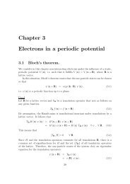
10 J. Roth - Solid State TheoryFigure 2: Within the Born-Oppenheimer approximation, the electrons move (arrow)in the static lattice potential of the ions (green) and interact with the other electronsthrough the Coulomb interaction (red). Due to the latter, the moving electron isrepelled by the electron located on the next site. It is energetically favorable ifthe depicted electron hops somewhere else, as indicated by the arrow. Hence, themovement of every electron is correlated with that of every other.Let us first notice, that if we multiply this equation by ψ ∗ 0 (x,R) and integrate overx, the first line above gives us an effective Schrödinger equation for the nuclei. Afterthis, we consider the non-adiabatic terms. For the first one we have∫d 3 xψ0∗ ∂ψ 0= 1 ∫∂∂R i 2 ∂R id 3 xψ ∗ 0 ψ 0 = 0 , (12)where we used the fact that without magnetic fields H = H ∗ so that the wavefunctioncan be chosen real, and that the total number of electrons cannot be changedby lattice vibrations.For the second non-adiabatic contribution, we assume the worst case that theelectrons are tightly bound to the nuclei, i.e., x i ≈ R j for some i and j. Then a

J. Roth - Solid State Theory 11crude estimate 1 gives− ¯h22MN∑∫j=1d 3 xψ0∗ ∂ 2 ψ 0∂R 2 ji≈ − ¯h22MN∑∫i=1d 3 xψ0∗ ∂ 2 ψ 0∂x 2 i= m M Ekin. el

12 J. Roth - Solid State Theory0.3 OverviewLet us now give a brief overview on what we will discuss in this lecture.The starting point, Hamiltonian (1), and the Born-Oppenheimer approximationare very general. We can use it to describe gases, liquids, or solids, as we do in thislecture. Moreover, we will only consider solids in the crystalline form, where theyare perfectly ordered in a periodic fashion. Actually, almost all materials becomesolid crystals at zero temperature. The notable exception is 4 He which, due tostrong quantum fluctuations of the Bose-Einstein condensated 4 He bosons, remainsa liquid. As we will see in this lecture, periodicity is a symmetry which, if cleverlyexploited, is of tremendous help. Hence, in the following chapter• Crystal structure.we will study this periodicity and the corresponding symmetry. We can also envisagethat we deal in this Section with the Hamiltonian (14) for the nuclei, wherewe neglect the movement of the nuclei, i.e., determine the equilibrium positions.However, since the determination of E0 el is such a formidable task, which we wouldneed to carry out for many nuclei positions, we will focus on the general symmetries.In the next chapter• Lattice vibrations.we will then include the motion of the nuclei around their equilibrium position.This way, we will discover elementary excitations of a solid: phonons. We will callelementary excitations, those modes of the system that at low enough energies (andhence, temperatures), can be considered as eigenmodes of the solid. These modeswill be real eigenmodes (i.e. modes with an infinite lifetime) only within certainapproximations (here disregarding the electron-phonon coupling). However, in thisway we will be able to understand the experiments and look for corrections byconsidering interactions among the elementary excitations, that in general will leadto a finite lifetime, as also seen in experiments. We will be more precise aboutthis in the coming chapters. Here we will have also the first encounter with secondquantization, much in the same way as in elementary quantum mechanics, whendiscussing the harmonic oscillator (creation and annihilation operators).Next we will focus on the electronic degrees of freedom described by Hamiltonian(6) within the Born-Oppenheimer approximation. First, we will consider theelectrons as non-interacting, and discuss• Electrons in a periodic potential.Since we know that electrons are charged, this may appear at a first sight as agross simplification. However, at the beginning of quantum mechanics, Sommerfeldconsidered electrons as non interacting particles and took only into account thefact that they obey the Fermi-Dirac statistics. In such a way he could explain thetemperature dependence of the specific heat in metals as well as their magnetic

J. Roth - Solid State Theory 13susceptibility. We will come to understand this apparent contradiction only later,when we discuss the effects of interaction. For the moment we will introduce theconcept of a band-structure, that is very useful to understand simple metals andsemiconductors.In order to complete the picture developed, we will come then, to consider• Interacting electrons.Here we will go deeper into the concepts of second quantization and develop a theoreticalframe that should allow us to deal in principle with fully interacting electrons.Unfortunately this goal was still not reached and different approaches are the subjectof current research. Nevertheless, the theoretical language developed here shouldbe useful to make contact with undergoing research work. On the other hand, itwill be useful to understand the solution of the contradiction mentioned above. Wewill see that in this case, the elementary excitation is the so-called quasiparticle,namely a fermionic excitation with spin 1/2 and charge −e that interacts weaklywith the other ones. This concept, introduced by Landau, explains the behavior ofmost metals. There are however, exceptions like one-dimensional systems or hightemperature superconductors, but they are the subject of more advanced lecturesand current research.The subjects above constitute the first half of these lectures. Students from theDiplomstudiengang may decide here, whether they continue, and make a full lecture,or they stop, and can combine this half-lecture with another elective one.The second half is devoted to different subjects that are important in the physicalunderstanding of solids. The first one is• Collective excitations.By them we denote those elementary excitations, that arise from the cooperativearrangement of electrons in long-lived modes like plasmons and excitons. We willdiscuss these in the general frame developed before as well as with simple picturesthat are helpful to understand their experimental manifestation.One of the most dramatic manifestations of quantum mechanics is the realizationof a state of matter, where transport of electric current takes place without losses,that is• Superconductivity.We will review here the phenomena, concepts, and theory of conventional superconductivity,a knowledge that is indispensable if we would like to understand a newform of superconductivity that is present in the so-called high temperature superconductors,where a different, new state of matter is suspected due to the evidencegiven by an increasing number of experiments. These new materials that were discoveredin 1986 by J. Bednorz and K.A. Müller, who received the Nobel Prize in

14 J. Roth - Solid State Theory1987, became one of the most important subjects of research in condensed matterphysics, and continue to be at the center of interest at present.Finally, the last chapter is devoted to• Magnetic properties.Magnetism known to most people due to the surprising effects that arise from theinteraction among magnets and of magnets with paramagnetic metals, plays a veryimportant role in new technologies like information storage devices. It also playsa central role in high temperature superconductivity and other so-called stronglycorrelated materials, where the properties, many of them still to be understood,are determined by strong interelectronic interactions. We will give here a survey ofdifferent phenomena related to magnetism, and of theoretical techniques developedto describe them.It is hoped that at the end of these lectures, a broad view of Solid State Physicsis achieved, such that students will be prepared to start their own research project inone of the research groups at Stuttgart, where condensed matter physics constitutesa major area of research.Addition: A very important subject in Solid State Theory is the understandingof transport phenomena, such that we will have a chapter devoted to• Transport properties.In fact the easiest experiments are in general related to transport properties, likeelectrical and thermal transport. The difficulty here is that most of the experimentsare performed out of equilibrium, a regime where well establishes theories are notavailable. Therefore, we will consider semiclassical theories that will give us a generaland intuitive understanding of transport phenomena. This will be a contrast to theformal theory we discussed in the previous chapters and it is hoped that in this waystudents well have a broad perspective of theoretical techniques and ideas to tackleproblems in the future.