17.874 Lecture Notes Part 3: Regression Model

Indeed, these properties are implied by (su±cient but not necessary), the assumption thaty; X are jointly normally distributed. See the properties of the conditional distributions insection 2.6.It is easy to see that this model implements the de¯nition of an e®ect above. Indeed, ifall of the assumptions hold we might even say the e®ect captured by the regression model iscausal.Two failures of causality might emerge.First, there may be omitted variables. Any variable X j that is not measured and includedin a model is captured in the error term ². An included variable might appear tocause (or not cause) y, but we have in fact missed the true relationship because we didnot hold X j constant. Of course, there are a very large number of potential omittedvariables, and the struggle in any ¯eld of inquiry is to speculate what those might beand come up with explicit measures to capture those e®ects or designs to remove them.Second, there may be simultaneous causation. X 1 might cause y, but y might also causeX 1 . This is a common problem in economics where prices at which goods are boughtand the quantities purchased are determined through bargaining or through markets.Prices and quantities are simultaneously determined. This shows up, in complicatedways, in the error term. Speci¯cally, the error term becomes recursive ²jX 1 necessarilydepends on ujy, the error term from the regression of X on y.Social scientists have found ways to solve these problems, involving \quasi-experiments"and sometimes real experiments. Within areas of research there is a lot of back and forthabout what speci¯c designs and tools really solve the problems of omitted variables andsimultaneity. The last third of the course will be devoted to these ideas.Now we focus on the tools for holding constant other factors directly.4

3.2. EstimationThe regression model has K + 1 parameters { the regression coe±cients and the errorvariance. But, there are n equations. The parameters are overdetermined, assumning n >K + 1. We must some how reduce the data at hand to devise estimates of the unknownparameters in terms of data we know.Overdetermination might seem like a nuisance, but if n were smaller than k +1 we couldnot hope to estimate the parameters. Here lies a more general lesson about social inquiry.Be wary of generalizations from a single or even a small set of observations.3.2.1. The Usual SuspectsThere are, as mentioned before, three general ideas about how use data to estimateparameters.1. The Method of Moments. (a) Express the theoretical moments of the random variablesas functions of the unknown parameters. The theoretical moments are the means, variances,covariances, and higher powers of the random variables. (b) Use the empirical moments asestimators of the theoretical moments { these will be unbiased estimates of the theoreticalmoments. (c) Solve the system of equations for the values of the parameters in terms of theempirical moments.22. Minimum Variance/Minimum Mean Squared Error (Minimum  ). (a) Express theobjective function of the sum squared errors as a function of the unknown parameters. (b)Find values of the parameters that minimize that function.3. Maximum Likelihood. (a) Assume that the random variables follw a particular densityfunction (usually normal). (b) Find values of the parameters that maximize the densityfunction.5

The total derivative, you may recall, is the partial derivative of y with respect to X j plusthe sum of partial derivatives of y with respect to all other variables, X k ,times the partialderivative of X k with respect to X j .If y depends on two X variables, then:dy @y @y dX 2= +dX 1 @X 1 @X 2 dX 1dy @y @y dX 1= +dX 2 @X 2 @X 1 dX 2Using the idea that the bivariate regression coe±cients measure the total e®ect of onevariable on another, we can write the bivariate regression estimates in terms of the partialregression coe±cient (from a multivariate regression) plus other partial regression coe±cientsand bivariate regression coe±cients. For simplicity consider a case with 2 X variables. Leta 1 and a 2 be the slope coe±cients from the regressions of y on X 1 and y on X 2 .Let b 1 andb 2 be the partial regression coe±cients from the multivariate regression of y on X 1 and X 2 .And let c 1 be the slope coe±cient from the regression of X 1 on X 2 and c 2 be the slope fromthe regression of X 2 on X 1 .We can express our estimates of the regression parameters in terms of the other coe±cients.Let r be the correlation between X 1 and X 2 .0 1 0 10 0 0 0µ (x2x2)(x1y) ¡(x1x2)(x2 y )b 0 x ) ( x 02 ¡ )2 1 x a 1 ¡a 2 c 11 (x0 x1)( x12 2=1¡r 2B C =B Cb 2 @ A @ A0 0 0(x1x1)(x2y) ¡(x1x)(a2¡a1 c20(x x )( x 01 x 2 ) ¡ ( x1¡r 21202 x1 y )0)1 x 2 2We can solve these two equations to express a 1 and a 2 in terms of b 1 and b 2 .a 1 = b 1 + b 2 c 1a 2 = b 2 + b 1 c 2 :This is estimated total e®ect (bivariate regression) equals the estimated direct e®ect of X j(partial coe±cient) on y plus the indirect e®ect of X j through X k .Another way to express these results is that multivariate regression can be simpli¯ed tobivariate regression, once we partial out the e®ects of the other variables on y and on X j .7

Suppose we wish to measure and display the e®ect of X 1 on y. Regress X 1 on X 2 ;:::X k .Regress y on X 2 ;:::X k . Take the residuals from each of these regressions, e(x 1 jx 2 ;:::x k )ande(yjx 2 ;:::x k ). The ¯rst vector of residuals equals the part of X 1 remaining after subtractingout the other variables. Importantly, this vector of residuals is independent of X 2 ; :::X k .Thesecond vector equals the part of y remaining after subtratcting the e®ects of X 2 ; :::X k {thatis the direct e®ect of X 1 and the error term ².Regress e(yjx 2 ;:::x k )on e(x 1 jx 2 ; :::x k ). This bivariate regression estimates the partialregression coe±cient from the multivariate regression, ¯1.Partial regression is very useful for displaying a particular relationship. Plotting the ¯rstvector of residuals against the second vector displays the partial e®ect of X 1 on y, holdingall other variables constant. In STATA partial regression plots are implmented through thecommand avplot. After performing a regression type the command avplot x1, where x1is the variable of interest.A ¯nal way to interpret regression is using prediction. The predicted values of a regressionare the values of the regression plane, ^y. These are estimates of E[yjX]. We mayvaryvaluesof any X j to generate predicted values. Typically, we consider the e®ect on y^ of a onestandarddeviation change in X j , say from 1/2 standard deviation below the mean of X to1/2 standard deviation above the mean.1Denote y^1 as the predicted value at x j = ¹x j + :5s j and y^0 as the predicted value atx0j = ¹x j ¡ :5s j . The matrix of all variables except x j is X (j ) and b (j) is the vector ofcoe±cients except b j . Choose any vector x (j) . A standard deviation change in the predictedvalues is:1 0 1 0y^1 ¡ y^0 =(b 0 + b j x j + x (0j)b (j) ) ¡ (b 0 + b j x 0 + x (j) b (j) )= b j (x j ¡ x j )= b j s j :jFor non-linear fucntions such variations are harder to analyze, because the e®ect of anyone variable depends on the values of the other variables. We typically set other variablesequal to their means.3.2.3. An Alternative Estimation Concept: Instrumental Variables.8

There are many other ways we may estimate the regression parameters. For example, wecould minimize the Mean Absolute Deviation of the errors.One important alternative to ordinary least squares estimation is instrumental variablesestimation. Assume that there is a variable or matrix of variables, Z, such that Z does notdirectly a®ect y, i.e., it is uncorrelated with ², but it does correlate strongly with X.The instrumental variables estimator is:b IV =(X 0 Z) ¡1 Z 0 y:This is a linear estimator. It is a weighted average of the y's, where the weights are of theformz ix) , in stead of x i(z (x i ¡¹ x) .i ¡z¹)(x i ¡ ¹ x)(x i ¡¹In the bivariate case, this esimator is the ratio of the slope coe±cient from the regressionof y on z to the slope coe±cient from the regression of x on z.This estimator is quite important in quasi-experiments, because, if we can ¯nd validinstruments, the estimator will be unbiased because it will be independent of omitted factorsin the least squares regression. It will, however, come at some cost. It is a noisier estimatorthan least squres.9

3.3. Properties of EstimatesParameter estimates themselves are random variables. They are functions of randomvariables that we use to make guesses about unknown constants (parameters). Therefore,from one study to the next, parameter estimates will vary. It is our hope that a given studyhas no bias, so if the study were repeated under identical conditions the results would varyaround the true parameter value. It is also hoped that estimation uses all available data ase±ciently as possible.We wish to know the sample properties of estimates in order to understand when wemight face problems that might lead us to draw the wrong conclusions from our estimates,such as spurious correlations.We also wish to know the sample properties of estimates in order to perform inferences.At times those inferences are about testing particular theories, but often our inferencesconcern whether we've built the best possible model using the data at hand. In this regard,we are concerned about potential bias, and will try to error on the side of getting unbiasedestimates.Erring on the side of safety, though, can cost us e±ciency. Test for the appropriatenessof one model versus another, then, depend on the tradeo® between bias and e±ciency.3.3.1. Sampling Distributions of EstimatesWe will characterize the random vector b with its mean, the variance, and the frequencyfunction. The mean is ¯, which means that it is unbiased. The variance is ¾ 2² (X 0 X) ¡1 ,whichis the matrix describing the variances and covariances of the estimated coe±cients. And thedensity function f(b) is approximated by the Normal distribution as n becomes large.The results about the mean and the variance stem from the regression assumptions.First, consider the mean of the parameter estimate. Under the assumption that ² 0 X = 0,10

the regression estimates are unbiased. That is, E[b] = ¯E[bjX] = E[(X 0 X) ¡1 X 0 y]= E[(X 0 X) ¡1 X 0 (X¯ + ²)] = (X 0 X) ¡1 X 0 X¯ + E(X 0 X) ¡1 X 0 ² = ¯This means that before we do a study we expect the data to yield a b of ¯. Of course, thedensity of any one point is zero. So another way to think about this is if we do repeatedsampling under identical circumstances, then the coe±cients will vary from sample to sample.The mean of those coe±cients, though, will be ¯.Second, consider the variance.V [b] = E[(b ¡ ¯)(b ¡ ¯) 0 ]= E[(¯ +(X 0 X) ¡1 X 0 ² ¡ ¯)(¯ +(X 0 X) ¡1 X 0 ² ¡ ¯) 0 ]= E[(X 0 X ¡1 X 0 ²)((X 0 X) ¡1 X 0 ²) 0 ]= E[X 0 X ¡1 X 0 ²² 0 X(X 0 X) ¡1 ]= ¾ 2 (X 0 X ¡1 X 0 X(X 0 X) ¡1 )= ¾ 2 X 0 X ¡1Here we have assumed the sphericality of the errors and the exogeneity of the independentvariables.The sampling distribution function can be shown to follow the joint normal. This followsfrom the multivariate version of the central limit theorem, which I will not present becauseof the complexity of the mathematics. The result emerges, however, from the fact that theregression coe±cients are weighted averages of the values of the random variable y, where thexiweights are of the form (xi. More formally, let b¡¹x) 2 n be the vector of regression coe±cientsestimated from a sample of size n.b n ! d N(¯; ¾ 2 ² (X 0 X ¡1 ))Of course, as n ! 1,(X 0 X ¡1 ) ! 0. We can see this in the following way. The elementsx 0jof (X 0 X ¡1 ) are, upto a signedterm, xkjX 0 Xj. The elements of the determinant are multiplesof the cross products, and as observations are added the determinant grows faster than anysingle cross product. Hence, each element approaches 0.Consider the 2x2 case.µ 00x 2 x 2 ; ¡x 1 x 2(X 0 X ¡1 1)=0 0 0 0x1 x 1 x 2 x 2 ¡ (x 1 x 2 ) 2 0 :¡ x 2 x 1 ; x 1 x 111

This may be rewritten asà 1¡1 !x0 0x 0 x (x0 2;1x1¡( x1 x ) 2 2 2 1x 1 x¡1=0 0 01 x 2 )0(x 0 x x0 0 1 x2=x x2 )¡(x ) ;2x2=x1x2 )¡(x10 0x x1 ¡(x x2 ) 2 = x0 x 21211 x 2Taking the limit of this matrix as n !1amounts to taking the limit of each element of thematrix. Considering each term, we see that the sum of squares in the denominators growwith the addition of each observation, while the numerators remain constant. Hence, eachelement approaches 0.Combined with unbiasedness, this last result proves consistency. Consistency meansthat the limit as n grows of the probability that an estimator deviates from the parameterof interest approaches 0. That is,lim n!1 Pr(jµ^ n ¡ µj)= 0A su±cient condition for this is that the estimator be unbiased and that the variance of theestimator shrink to 0. This condition is called convergence in mean squared error, and is animmediate application of Chebychev's Inequality.Of course, this means that the limiting distribution of f(b) shrinks to a single point,which is not so good. So the normality of the distribution of b is sometimes written asfollows:p n(bn ¡ ¯) » N(0;¾ 2 ² Q ¡1 );1where Q = n(X 0 X), the asymptotic variance covariance matrix of X's.112We may consider in this the distribution of a single element of b.2b j » N(¯j ;¾ ² a jj );where a jj is the jth diagonal element of (X 0 X) ¡1 .Hence, we can construct a 95 percent con¯dence interval for any parameter ¯j using thenormal distribution and the above formula for the variance of b j . The standard error isq¾2² a jj . So, a 95 percent con¯dence interval for a single parameter is:b j § 1:96 q ¾ 2 ² a jj12

.The instrumental variables estimator provides an interesting contrast to the least squaresestimator. Let us consider the sampling properties of the Instrumental Variables estimator.E[b IV ]= E[(X 0 Z) ¡1 (Z 0 y)] = E[(X 0 Z) ¡1 (Z 0 (X¯ + ²)]= E[(X 0 Z) ¡1 (Z 0 X)¯ +(X 0 Z) ¡1 (Z 0 ²))] = E[¯ +(X 0 Z) ¡1 (Z 0 ²))] = ¯The instrumental variables estimator is an unbiased estimator of ¯.The variance of the instrumental variables estimator is:0V [b IV ]= E[(b IV ¡ ¯)(b IV ¡ ¯) 0 ]= E[(X Z) ¡1 (Z 0 ²))((X 0 Z) ¡1 (Z 0 ²)) 0 ]2= E[(X 0 Z) ¡1 (Z 0 ²²Z((X 0 Z) ¡1 ]=(X 0 Z) ¡1 (Z 0 ¾ ² IZ((X 0 Z) ¡12= ¾ ² (X 0 Z) ¡1 (Z 0 Z((X 0 Z) ¡1 :As with the least squares estimator the instrumental variables estimator will follow anormal distribution because the IV estimator is a (weighted) sum of the random variables,y.3.3.2. Bias versus E±ciency3.3.2.1. General E±ciency of Least SquaresAn important property of the Ordinary Least Squares estimates is that they have thelowest variance of all linear, unbiased estimators. That is, they are the most e±cient unbiasedestimators. This result is the Gauss-Markov Theorem. Another version arises as a propertyof the maximum likelihood estimator, where the lower bound for the variances of all possible2consistent estimators is ¾ ² (X 0 X) ¡1 .This implies that the Instrumental Variables estimator is less e±cient than the OrdinaryLeast Squares estimator. To see this, consider the bivariate regression case.2¾ ²V [b] = P(x x) 2 i ¡ ¹13

2 P¾ (zi ¡ z¹) 2V [b ²IV ]= P(x i ¡ x)(z ¹ i ¡ z¹)P P(zi ¡z¹)2 P (xi¡¹ x)Comparingthese twoformulas: V [b 2IV ]=V [b] = ( . This ratio is the inverse(x i ¡ x)(z ¹ i ¡z¹)of the square of the correlation between X and Z. Since the correlation never exceeds 1, weknow the numerator must be larger than the denominator. (The square of the correlation isknown to be less than 1 because of the Cauchy-Schwartz inequality.)3.3.2.2. Sources of Bias and Ine±ciency in Least SquaresThere are four primary sources of bias and inconsistency in least squares estimates: measurementerror in the independent variables, omitted variables, non-linearities, and simultaneity.We'll discuss two of these cases here { speci¯cation of regressors (omitted variables)and measurement error.Measurement Error.Assume that X ¤ is the true variable of interest but we can only measure X = X ¤ + u;where u is a random error term. For example, suppose we regress the actual share of thevote for the incumbent president in an election on the job approval rating of the incumbencypresident, measured in a 500 person preelection poll the week before the election. Galluphas measured this since 1948. Each election is an observation. The polling data will havemeasurement error based on random sampling inherent in surveys. Speci¯cally, the varianceof the measurement error is p(1 ¡p)n,where p is the percent approving of the president.Another common source of measurement error arises from typographical errors in datasets.Keypunching errors are very common, even in data sets distributed publicly through reputablesources such as the Interuniversity Consortium for Political and Social Research. Forexample, Gary King, Jim Snyder, and others who have worked with election data estimatethat about 10 percent of the party identi¯cation codes of candidates are incorrect in someof the older ICPSR datasets on elections.Finally, some data sources are not very reliable, or estimates must be made. This is14

common in social and economic data in developing economies and in data on wars.If we regress y on X, the coe±cient is a function of both the true variable X ¤ and theerror term. That isb =P nPnPni=1(x x)(y i ¡ y¹) i=1(x ¤ i ¡ x ¹ ¤ i ¡ ¹+ u i ¡ u)(y ¹ i ¡ y¹)=x) 2 n ¹i=1 (x i ¡ ¹Pi=1 (x¤ i ¡ x ¤ + u u) 2 i ¡ ¹P n ¹P n= P n P n P ni=1 (x i ¤ ¡ x ¤ )(y i ¡ y¹)+ i=1 (u i ¡ ¹u)(y i ¡ y¹)i=1(x ¤ i ¡ x ¹ ) 2 + i=1(u i ¡ u) ¹ + i=1(x ¤ x ¤ i ¡ ¹ )(u i ¡ ¹u)This looks like quite a mess.A few assumptions are made to get some traction. First, it is usually assumed that u and² and that u and X ¤ are uncorrelated. If they are correlated, things are even worse. Second,the u i 's is assumed to be uncorrelated with one another and to have constant variance.Taking expected values of b will be very di±cult, because b is a function of the ratioof random variables. Here is a situation where Probability Limits (plim's) make life easier.Because plims are limits, they obey the basic rules of limits. The limit of a sum is the sumof the limit and the limit of a ratio is the ratio of the limits. Divide the top and bottom ofb by n. Now consider the probability limit of each element of b:1 X nn i=1plim (x ¤ ¡ x¹¤ ) 2 = ¾ 2inn1 X 1 X¹ ¹ ¹i i xni=1ni=1plim (x ¤ ¡ x ¤ )(y i ¡ y¹) = plim (x i ¤ ¡ x ¤ )(¯x ¤ ¡ x ¤ )= ¯¾ 21 X nplim (x i ¤ ¡ x¹¤ )(u i ¡ ¹u)= 0xn i=1n1 Xn i=1We can pull these limits together as follows:plim (u u) 2 = ¾ 2i ¡ ¹ uplimb =¯¾ 2 x ¾ 2x= ¯¾ 2 + ¾ 2 ¾ 2 + ¾ 2x u x u

typical, but it is possible also to reverse signs or in°ate the coe±cients. In non-linear models,such as those using the square of X, the bias terms become quite substantial and even moretroublesome.The best approach for eliminating measurement error is cleaning the dataset. However,it is possible to ¯x some measurement error using instrumental variables. One approach isto use the quantiles or the ranks of the observed X to predict the observed X andthenusethe predicted values in the regression predicting y. The idea behind this is that the ranks ofX are correlated with the underlying true values of X, i.e., X ¤ but not with u or ².These examples of measurement error assume that the error is purely random. It may notbe. Sometimes measurement error is systematic. For example, people underreport sociallyundesirable attitudes or behavior. This is an interesting subject that is extensively studiedin public opinion research, but often understudied in other ¯elds. A good survey researcher,for example, will tap into archives of questions and even do question wording experimentsto test the validity and reliability of instruments.Choice of Regressors: omitted and Included Variables.The struggle in most statistical modeling is to specify the most appropriate regressionmodel using the data at hand. The di±culty is deciding which variables to include and whichto exclude. In rare cases we can be guided by a speci¯c theory. Most often, though, we havegathered data or will gather data to test speci¯c ideas and arguments. From the data athand what is the best model?There are three important rules to keep in mind.1. Omitted Variables That Directly A®ect Y And Are Correlated With X Produce Bias.The most common threat to the validity of estimates from a multivariate statisticalanalysis is omitted variables. omitted variables a®ect both the consistency and e±ciency ofour estimates. First and foremost, they create bias. Even if they do not bias our results, we16

often want to control for other factors to improve e±ciency.To see the bias due to omitted variables assume that X is a matrix of included variablesand Z is a matrix of variables not included in the analysis. The full model isy = X¯X + Z¯z + ²:Suppose that Z is omitted. Obviously we can't estimate the coe±cient ¯ .Will the otherzcoe±cients be biased? Is there a loss of e±ciency?Let b x be the parameter vector estimated when only the variables in the matrix X areincluded. Let ¯X bet the subset of coe±cients from the true model on the included variables,X. The model estimated iswhere u = Z¯ z + ².y = X¯X + u;0 0 X) ¡1 0 0E[b X ]= E[(X 0 X) ¡1 X y] = E[(X X X¯X +(X 0 X) ¡1 X u]= ¯ + E[(X 0 X) ¡1 X 0 Z¯ z ]+ E[(X 0 X) ¡1 X 0 ²]= ¯X + ¦ 0 ¯ z ;Xzxwhere ¦ zx is a matrix of coe±cients from the regression of the columns of Z on the variablesin X.This is an extremely useful formula. There are two important lessons to take away.First, omitted variables will bias regression estimates of the included variables (and leadto inconsistency) if (1) those variables directly a®ect Y and (2) those variables are correlatedwith the included variables (X). It is not enough, then, to object to an analysis that thereare variables that have not been included. That is always true. Rather, science advancesby conjecturing (and then gathering the data on) variables that a®ect y directly and arecorrelated with X . I think the latter is usually hard to ¯nd.Second, we can generally sign the bias of omitted variables. When we think about thepotential problem of an omitted variable we usually have in mind the direct e®ect that it17

likely has on the dependent variable and we might also know or can make a reasonable guessabout the correlation with the included variables of interest. The bias in an included variablewill be the direct e®ect of the omitted variable on y times the e®ect of the included variableon the excluded variable. If both of those e®ects are positive or both are negative then theestimated e®ect of X on Y will be biased up { it will be too large. If one of these e®ects isnegative and the other positve then the estimate e®ect of X on Y will be biased downward.2. E±ciency Can Be Gained By Including Variables That Predict Y But Are UncorrelatedWith X.2A straightforward analysis reveals that the estimated V [b X ]= s e (X 0 X) ¡1 . So1good. But the variance of the error term is in°ated. Speci¯cally, s 2 =0e n¡Ku u. Because0 2u = Z¯Z + ², E[u 0 u=(n ¡ K)] = ¯ZZ 0 Z¯Z=(n ¡ K) + ¾²2 >¾ ² . In fact, the estimatedresidual variance is too large by the explained or model sums of squared errors for theomitted variables.This has an interesting implication for experiments. Randomization in exp eriments guaranteesunbiasedness. But, we still want to control for other factors to reduce noise. In fact,combining regression models in the data analysis is a powerful way to gain e±ciency (andreduce the necessary sample sizes) in randomized experiments.Even in observational studies we may want to keep in a model a variable whose inclusiondoes not a®ect the estimated value of the parameter of a variable of interest if the includedvariable strongly a®ects the dependent variable. Keeping such a variable captures some ofthe otherwise unexplained error variance, thereby reducing the estimated variance of theresiduals. As a result, the size of con¯dence intervals will narrow.farso3. Including Variables That Are Unrelated To Y and X Loses E±ciency (Precision), AndThere IsNo BiasFrom Their ExclusionThat there is no bias can be seen readily from the argument we have just made.18

The loss of e±ciency occurs because we use up degrees of freedom. Hence, all varianceestimates will be too large.Simply put, parsimonious models are better.COMMENTS:a. Thinking through the potential consequences of omitted variables in this manner is veryuseful. It helps you identify what other variables will matter in your analysis and why,and it helps you identify additional information to see if this could be a problem. Itturns out that the ideological ¯t with the district has some correlation with the vote,but it is not that strong. The reason is there is relatively little variation in ideological¯t that is not explained by simple knowledge of party. So this additional informationallows us to conjecture (reasonably safely) that, although ideological ¯t could be aproblem, it likely does not explain the substantial bias in the coe±cients on spending.b.The general challenge in statistical modeling and inference is deciding how to balance possiblebiases against possible ine±ciencies in choosing a particular speci¯cation. Naturally,we usually wish to err on the side of ine±ciency. But, these are choices wemake on the margin. As we will see statistical tests measure whether the possible improvementin bias from one model outweighs the loss of e±ciency compared to anothermodel. This should not distract from the main objective of your research, which is to¯nd phenomena and relationships of large magnitude and of substantive importance.Concern about omitted Variable Bias should be a seed of doubt that drives you tomake the estimates that you make as good as possible.3.3.3. ExamplesModel building in Statistics is really a progressive activity. We usually begin with interestingor important observations. Sometimes those originate in a theory of social behavior,19

and sometimes they come from observation of the world. Statistical analyses allow us tore¯ne those observations. And sometimes they lead to a more re¯ned view of how socialbehavior works. Obvious problems of measurement error or omitted variables exist whenthe implications of an analysis are absurd. Equally valid, though, are arguments that suggesta problem with a plausible result. Here we'll consider four examples.1. Incumbency AdvantagesThe observation of the incumbency advantage stems from a simple di®erence of means.From 1978 to 2002, the average Demcoratic vote share of a typical U.S. House Democraticincumbent is 68%; the average Democratic vote share a typical U.S. House Republicanincumbent is 34The incumbency advantage model is speci¯ed as follows. The vote for the Democraticcandidate in district i in election t equals the normal party vote, N i , plus a national partytide, ® t , plus the e®ect of incumbency. Incumbency is coded I it = +1 for DemocraticIncumbents, I it = ¡1 for Republican Incumbents, and I it =0 for Open Seats.V it = ® t + N i + ¯I it + ² itControlling for the normal vote and year tides reduces the estimated incumbency e®ectto about 7 to 9 percentage oints.2. Strategic Retirement and the Incumbency AdvantageAn objection to models of the incumbency advantage is that incumbents choose to stepdown only when they are threatened, either by changing times, personal problems, or anunusually good challenger. The reasons that someone retires, then, might depend on factorsthat the researcher cannot measure but that predict the vote { omitted variables. This wouldcause I to be correlated to the regression error u. The factors that are thought to a®ect theretirement decisions and the vote are negatively correlated with V and negatively correlatedwith I (making it less likely to run). Hence, the incumbency advantage may be in°ated.20

3. Police/Prisons and CrimeThe theory of crime and punishment begins with simple assumptions about rationalbehavior. People will comit crimes if the likelihood of being caught and the severity of thepunishment are lower than the bene¯t to the crime. A very common observation in thesociology of crime is that areas that have larger numbers of police or more people in prisonhave higher crime rates.4. Campaign Spending and VotesResearchers measuring the factors that explain House election outcomes include variousmeasures of electoral competition in explaining the vote. Campaign Expenditures, and theadvertising they buy, are thought to be one of the main forces a®ecting election outcomes.A commonly used model treats the incumbent party's share of the votes as a functionof the normal party division in the congressional district, candidate characteristics (such asexperience or scandals), and campaign expenditures of the incumbent and the challenger.Most of the results from such regressions make sense: the coe±cient on challenger spendingand on incumbent party strength make sense. But the coe±cient on incumbent spendinghas the wrong (negative) sign. The naive interpretation is that the more incumbents spendthe worse they do.One possibile explanation is that incumbents who are unpopular and out of step withtheir districts have to spend more in order to remain in place. Could this explain the incorrectsign? In this account of the bias in the spending coe±cients there is a positive correlationbetween the omitted variable, \incumbent's ¯t with the district," and the included variable,\incumbent spending." Also, the incumbent's ¯t with the district likely has a negative directe®ect on the vote. The more out-of-step an incumbent is the worse he will do on electionday. Hence, lacking a measure of \¯t with the district" might cause a downward bias.Biases3.3.3. General strategies for Correcting for Omitted Variables and Measurement Error21

1. More Data, More Variables. Identify relevant omitted variables and then try to collectthem. This is why many regression analyses will include a large number of variables thatdo not seem relevant to the immediate question. They are included to hold other thingsconstant, and also to improve e±ciency.2. Multiple Measurement.Two sorts of use of multiple measurement are common.First, to reduce measurement error researchers often average repeated measures of avariable or construct an index to capture a \latent" variable. Although not properly a topicfor this course, factor analysis and muti-dimensional scaling techniques are very handy forthis sort of data reduction.Second, to eliminate bias we may observe the \same observation" many times. Forexample, we could observe the crime rate in a set of cities over a long period of time. If theomitted factor is one that due to factors that are constant within Panel models. omittedVariables as Nuisance Factors. Using the idea of "control in the design."3. Instrumental Variables.Instrumental variables estimates allow researchers to purge the independent variable ofinterest with its correlation with the omitted variables, which cause bias. What is di±cult is¯nding suitable variables with which to construct instruments. We will deal with this matterat length later in the course.22

3.4. Prediction3.4.1. Prediction and InterpretationWe have given one interpretation to the regression model as an estimate of the partialderivatives of a function, i.e., the e®ects of a set of independent variables holding constantthe values of the other independent variables. In constructing this de¯nition we began withthe de¯nition of an e®ect as the di®erence in the conditional mean of Y across two distinctvalues of X. And, a causal e®ect assumes that we hold all else constant.Another important way to interpret conditional means and regressions is as predictedvalues. Indeed, sometimes the goal of an analysis is not to estimate e®ects but to generatepredictions. For example, one might be asked to formulate a prediction about the comingpresidential election. A common sort of election forecasting model regresses the incumbentpresident's vote share on the rate of growth in the economy plus a measure of presidentialpopularity plus a measure of party identi¯cation in the public. Based on elections since 1948,that regression has the following coe±cients:Vote = xxx + xxxGrowth + xxxP opularity + xxxxP arty:We then consider plausible values for Growth, Popularity, and Partisanship to generatepredictions about the Vote.For any set of values of X, say x 0 , the most likely value or expected value of Y isy 0 = E[Y jx = x 0 ]. This value is calculated in a straightforward manner from the estimatedregression. Let x 0 be a row vector of values of the independent variables for which a0 0 0prediction is made. I.e., x 0 =(x 1 ; x 2 ;:::x k ). The predicted value is calculated asX K0 0y^ = x 0 b = b 0 + b j x j :j=1It is standard practice to set variables equal to their mean value if no speci¯c value is ofinterest in a prediction. One should be somewhat careful in the choice of predicted valuesso that the value does not lie too far out of the set of values on which the regression wasoriginally estimated.23

Consider the presidential election example. Assume a growth rate of 2 percent, a Popularityrating of 50 percent, and a Republican Party Identi¯cation of 50 Percent (equalsplit between the parties), then Bush is predicted to receive xxx percent of the two-partypresidential vote in 2004.The predicted value or forecast is itself subject to error. To measure the forecast errorwe construct the deviation of the observed value from the \true" value, which we wish topredict. The true value is itself a random variable: y 0 = x 0¯ + ² 0 . The prediction or forecasterror is the deviation of the predicted value from the true value:0 0e = y ¡ y^0 = x 0 (¯ ¡ b)+ ² 0The varince of the prediction error isV [e ]= ¾ 2 + V [(x 0 (¯ ¡ b)] = ¾ 2 +(x 0 E[(¯ ¡ b)(¯ ¡ b) 0 ]x 0 )= ¾ 2 + ¾ 2 ² (x 0 (X 0 X) ¡1 x 0 )0 0 0² ² ²We can use this last result to construct the 95 percent con¯dence interval for the predictedvalue:q0y^ § 1:96 V [e 0 ]As a practical matter this might become somewhat cumbersome to do. A quick wayto generate prediction con¯dence intervals is with an \augmented" regression. Suppose wehave estimated a regression using n observations, and we wish to construct several di®erentpredicted values based on di®erent sets of values for X, say X 0 . A handy trick is to addthe matrix of values X 0 to the bottom of the X matrix. That is add n 0 observations toyour data set for which the values of the indepedent variables are the appropriate values ofX 0 . Let the dependent variable equal 0 for all of these values. Finally, add n 0 columns toyour dataset that equal -1 for each new observation. Now regress y on X and the new set ofdummy variables.The resulting estimates will reproduce the original regression and will have coe±cient estimatesfor each of the independent variables. The coe±cients on the dummy variables equal24

the predicted values and the standard errors of these estimates are the correct predictionstandard errors.As an example, consider the analysis of the relationship between voting weights andposts in parliamentary governments. Let's let regression calculate the predicted values andstandard errors for 6 distinct cases: Voting Weight = .25 and Formateur, Voting Weight= .25 and Not Formateur, Voting Weight = .35 and Formateur, Voting Weight = .35 andNot Formateur, Voting Weight = .45 and Formateur, and Voting Weight = .45 and NotFormateur. First, I ran the regression of Share of Posts on Share of Voting Weight plus anIndicator variable of The Party that formed the government (Formateur). I then ran theregression with 6 additional observations, constructed as described above. Below are theestimated coe±cients and standard errors (constants not reported).Using Augmented Regression To Calculate Predicted ValuesVariable Coe®. (SE) Coe®. (SE)Voting WeightFormateurD 1 (.25, 1)D 2 (.25, 0)D 3 (.35, 1)D 4 (.35, 0)D 5 (.45, 1)D 6 (.45, 0).9812 (.0403).2300 (.0094){{{{{{.9812 (.0403).2300 (.0094).5572 (.0952).3272 (.0952).6554 (.0953).4253 (.0955).7535 (.0955).5235 (.0960)3.4.2. Model CheckingPredicted values allow us to detect deviations from most of the assumptions of the regressionmodel. The one assumption we cannot validate is the assumption that X and ²are uncorrelated. The residual vector, e, is de¯ned to be orthogonal to the independentvariables, X: e 0 X = 0. This implies that e 0^y = e 0 Xb = 0. This is a restriction, so wecannot test how well the data approximate or agree with this assumption.The other assumptions { linearity, homoskedasticity, no autocorrelation, and normality{ are readily veri¯ed, and ¯xed. A useful diagnostic tool is a residual plot. Graph the25

esiduals from a regression against the predicted values. This plot will immediately showmany problems, if they exist. We expect an elliptical cloud centered around e =0.If the underlying model is non-linear, the residual plot will re°ect the deviations of thedata from a straightline ¯t through the data. Data generated from a quadratic concavefunction will have negative residuals for low values of ^y, then positive for intermediate valuesof y, ^ then negative for large values of y. ^If there is heteroskedasticity, the residual plot will show deviations non-constant deviationsaround e = 0. A common case arises when the residual plot looks like a funnel. This¯situation means that the e®ects are multiplicative. That is the model is y = ®X ² (where² takes only positive values), not y = ® + ¯X + epsilon. This is readily ¯xed by takinglogarithms, so that the model becomes: y = log(®)+ ¯log(X )+ log(²).A further plot for measuring heteroskedasticity is of e 2 against ^y, against a particular Xvariable, or against some other factor, such as the \size" of the unit. In this plot e 2 servesas the estimate of the variance. This is an enlightening plot when the variance is a functionof a particular X or when we are dealing with aggregated data, where the aggregates consistof averages of variables across places of di®erent populations.To detect autocorrelation we use a slightly di®erent plot. Suppose the units are indexed bytime, say years, t. We may examine the extent of autocorrelation by taking the correlationsbetween observations that are s units apart:P Tt=1 e te t¡sr s = P T 2t=1 e tThe correlation between an observation and the previous observation is r 1 . Thisiscalled¯rst-order autocorrelation. Another form of autocorrelation, especially in monthly economicdata, is seasonal variation, which is captured with s = 12.It is instructive to plot the estimated autocorrelation against s, where s runs from 0 toa relatively large number, say 1/10th of T.What should this plot look like? At s = 0, the autocorrelation parameter is just ¾ 2 = ²¾ 2 u1¡½ 2 . The values of r s for s > 0 depends on the nature of the autocorrelation structure.26

Let's take a closer look.The most basic and commonly analyzed autocorrelation structure involves an autoregressionof order 1 (or AR-1). Let u t be an error term that is independent of ² t . First-orderautocorrelation in ² is of the form:² t = ½² t¡1 + u tThevarianceof ² t follows immediately from the de¯nition of the variance:¾ 2 ² = E[(½² t¡1 + u t )(½² t¡1 + u t )] = ½ 2 ¾ 2epsison + ¾2 uSolving for ¾ 2epsilon : ¾ 2¾ 2²u= :(1 ¡ ½ 2 )To derive, the correlation between t and t ¡ s, we must derive the covariance ¯rst. For s = 1,the covariance between two observations isE[² t ² t¡1 ]= E [(½² t¡1 + u t )² t¡1 ]= ½¾ 2²Using repeated substitutions for ² we ¯nd that for an AR-1:tE[² t ² t¡s ]= ½ s ¾ 2²Now, we can state what we expect to observe in the r s when the residuals contain ¯rstorderautocorrelation:Cov(² t ;² t¡s ) ½ s 2¾½ ²s = q = = ½ sV (² ¾ 2t )V (² t¡1 ) ²There are two patterns that may appear in the autocorrelation plot, depending on the signof ½. If ½> 0, the plot should decline exponentially toward 0. For examle, suppose ½ = :5,then we expect r 0 =1, r 1 = :5, r 2 = :25, r 3 = :125, r 4 = :0625, r 5 = :03125. If ½ < 0, theplot will seesaw, converging on 0. For example, suppose ½ = ¡:5, then we expect r 0 =1,r 1 = ¡:5, r 2 = :25, r 3 = ¡:125, r 4 = :0625, r 5 = ¡:03125.Higher order auto-correlation structures { such as ² t = ½ 1 ² t¡1 + ½ 2 ² t¡2 + u t {lead tomore complicated patterns. We may test for the appropriateness of a particular structure27

y comparing the estimated autocorrelations, r s , with the values implied by a structure. Forexample, we may test for ¯rst order autocorrelation by comparing the observed r 's with sthose implied by the AR-1 model when ½^ = r 1 .A simple rule of thumb applies for all autocorrelation structures. If r s

3.5. Inference3.5.1. General Framework.Hypotheses.What is an hypothesis? An hypothesis is a statement about the data derived from anargument, model, or theory. It usually takes the form of a claim about the behavior ofparameters of the distribution function or about the e®ect of one variable on another.For example, a simple argument about voting holds that in the absence of other factors,such as incumbency, voters use party to determine their candidate of choice. Therefore,when no incumbent is on the ticket, an additional one-percent Democratic in an electoraldistrict should translate into one-percent higher Democratic vote for a particular o±ce. Ina regression model, controlling for incumbency, the slope on the normal vote ought to equalone. Of course there are a number of reasons why this hypothesis might fail to hold. Theargument itself might be incorrect; there may be other factors beside incumbency that mustbe included in the model; the normal vote is hard to measure and we must use proxies, whichintroduce measurement error.In classical statistics, an hypothesis test is a probability statement. We reject an hypothesisif the probability of observing the data given that the hypothesis is true is su±cientlysmall, say below .05. Let T be the vector of estimated parameters and µ be the true parametersof the distribution. Let µ 0 be the values of the distribution posited by the hypothesis.Finally, let § be the variance of T. If the hypothesis is true, then µ = µ 0 . If the hypothesisis true, then the deviation of T from µ 0 should look like a random draw from the underlyingdistribution, and thus be unlikely to have occured by chance.What we have just described is the size of a test. We also care about the power of a test.If µ 0 is not true, what is the probability of observing a su±ciently small deviation that wedo not reject the hypothesis? This depends on sample size and variance of X.29

Tests of a Single Parameter.We may extend the framework for statistical tests about means and di®erences of meansto the case of tests about a single regression coe±cient. Recall that the classical hypothesistest for a single mean was:sPr(j¹x ¡ ¹ 0 j > t ®=2;n¡1 p n) < ®Because ¹x is the sum of random variables, its distribution is approximately normal. However,because we must estimate the standard deviation of X, s, the t-distribution is used as thereference distribution for the hypothesis test. The test criterion can be rewritten as follows.x¡¹ 0 jWe reject the hypothesis if j¹ >t ®=2;n¡1 .s= p nThere is an important duality between the test criterion above and the con¯dence interval.The test criterion for size .05 may be rewritten as:¾¾Pr(¹ x ¡ t :025;n¡1 p :95n nSo, we can test the hypothesis by ascertaining whether the hypothesized value falls insidethe 95 percent con¯dence interval.Now consider the regression coe±cient, ¯. Suppose our hypothesis is H : ¯ = ¯ 0 . Acommon value is ¯ 0 = 0 { i.e., no e®ect of X on Y. Like the sample average, a singleregression parameter follows the normal distribution, because the regression parameter isP ¾ 2²the sum of random variables. The mean of this distribution is ¯ and the variance ,(x x) 2 i ¡¹in the case of a bivariate regression, or, more generally, ¾ 2 ² a jj ,where a jj is the jth diagonalelement of the matrix (X 0 X) ¡1 .The test criterion for the hypothesis states the following. If the null hypothesis is true,then we expect that the probability of a large standardized deviation b from ¯0 will beunlikely to have occurred by chance:Pr(jb ¡ ¯0 j > t ®=2;n¡K s p a jj ) < ®As with the sample mean, this test criterion can be expressed as follows. We reject thejb¡¯ 0 jhypothesized value if sp ajj>t ®=2;n¡K .30

The Wald Criterion.The general framework for testing in the multivariate context is a Wald Test. Constructa vector of estimated parameters and a vector of hypothesized parameters. Generically, wewill write these as T and µ 0 , because they may be functions of regression coe±cients, notjust the coe±cients themselves. De¯ne the vector of deviations of the observed data fromthe hypothesized data as d = bfT ¡ µ 0 . This is a vector of length J.What is the distribution of d? Under the null hypothesis, E [d] = 0 and V [d] = V[T] =§. The Wald statistic is:W = d 0 § ¡1 d:Assuming d is normally distributed, the Wald Statistic follows the  2 distribution with Jdegrees of freedom.Usually, we do not know §, and must estimate it. Substituting the estimated value of§ and making an appropriate adjustment for the degrees of freedom, we arrive at a newstatistic that follows the F distribution. The degrees of freedom are J and n ¡ K, which arethe number of restrictions in d and the number of free pieces of information available afterestimation of the model.In the regression framework, we may implement a test of a set of linear restrictions onthe parameters as follows. Suppose the hypotheses take the form that linear combinationsof various parameters must equal speci¯c constants. For example,¯ 1 =0¯ 2 =3and¯ 4 + ¯ 3 =1. Wecan specify thehypothesis asR¯ = q31

Where R is a matrix of numbers that correspond to the parameters in the set of linearequations found in the hypothesis; ¯ is the vector of coe±cients in the full model (lengthK), and q is an appropriate set of numbers. In the example, suppose there are 5 coe±cintsin the full model: 0 ¯ 10 1 1 0 110000 ¯ 20B C B C B CB C@ A 1R¯ = @ 01000 A B ¯3 C @ 3 A00110 ¯4The deviation of the estimated value from the true value assuming the hypothesis is trueisd = Rb ¡ R¯ = Rb ¡ qIf the hypothesisiscorrect: E[d] = E[Rb ¡ q]= 0.¯50 0V [d] = E[dd ]= E[(Rb ¡ R¯)(Rb ¡ R¯) 0 ]= E[R(b ¡ ¯)(b ¡ ¯) 0 R ]Because R is a matrix of constants:0 2 0V [d]= RE[(b ¡ ¯)(b ¡ ¯) 0 ]R = R¾ ² X 0 X) ¡1 RBecause we usually have to estimate the variance of ² the Wald statistic isF =(Rb ¡ q) 0 [R(X 0 X) ¡1 R 0 ](Rb ¡ q)=Je 0 e=(n ¡ K)Another way to write the F-statistic for the Wald test is as the percentage loss of ¯t.Suppose we estimate two models. In one model, the Restricted Model, we impose thehypothesis, and on the other model, the Unrestricted Model, we impose no restrictions. TheF-test for the Wald criterion can be written ase0 0R e R ¡ e u e u =JF =e0u e u =(n ¡ K)Denote the residuals from these models as e R and e U . We can write the residuals from therestricted model in terms of the residuals from the unrestricted model: e R = y ¡ Xb R =32

y ¡ Xb U ¡ X(b R ¡ b U )= e U ¡ X(b R ¡ b U ). The sum of squares residuals from the re-stricted model is e0R e R =(e U ¡ X(b R ¡ b U )) 0 (e U ¡ X(b R ¡ b U ))0 0= e U e U ¡ (b R ¡ b U ) 0 X 0 X(b R ¡ b U )= e U e U ¡ (Rb U ¡ q) 0 (R(X 0 X) ¡1 R 0 )(Rb U ¡ q) So,the di®erence in the sum of squares between the restricted and the unrestricted model equalsthe numerator of the Wald test.There are two other important testing criteria { likelihood ratio statistics and lagrangemultiplier tests. These three are asymptotically the same. The Wald criterion has bettersmall sample properties, and it is easy to implement for the regression model. We will discusslikelihood ratio statistics as part of maximum likelihood estimation.33

3.5.2. ApplicationsThree important applications of the Wald Test are (1) tests of speci¯c hypotheses, (2)veri¯cation of choice of a speci¯cation, and (3) tests of bias reduction in causal estimates,speci¯cally OLS versus IV. All three amount to comparing the bias due to the more parsimonioushypothesized model against the e±ciency gain with that model.i. Hypothesis Tests: Seats and Votes in England, 1922-2002.The Cube Law provides an excellent example of the sort of calculation made to test aconcrete hypothesis. The Cube Law states that the proportion of seats won varies as thecube of the proportion of votes won:µ 3S V= :(1 ¡ S) 1 ¡ VWe may implement this in a regression model as follows. This is a multiplicative modelwhich we will linearize using logarithms. There are really two free parameters { the constantterm ® and the exponent ¯.µ SVlog( )= ® + ¯log(1 ¡ S) 1 ¡ VFor English Parliamentary elections from 1922 to 2002, the graph of the log of the oddsof the Conservatives winning a seat (labelled LCS) versus the log of the odds of the Conservativeswinning a vote (labelled LCV) is shown in the graph. The relationship looks fairlylinear.Results of the least squares regression of LCS on LCV are shown in the table. The slopeis 2.75 and the intercept is -.07. Tests of each coe±cient separately show that there we wouldsafely accept the hypothesis that ¯ 0 =0 and ¯ 1 = 3, separately. Speci¯cally, the t-test ofwhether the slope equals 3 is 2:75¡3 =1:25, which has a p-value of .25. The t-test of whether:20the constant equals 0 is ¡:07¡0 = ¡1:4, which has a p-value of .18.:0534

Regression Example:Cube Law in England, 1922-2002Y = Log of the Odds Ratio of Conservative SeatsX = Logof the Odds Ratioof Conservative VotesVariable Coe®. (SE) t-testLCV 2.75 (.20) .25/.2 = 1.25(p = .24)Constant -0.07 (.05) -.07/.05 = -1.4(p = .18)N 21R 2 .91MSE .221F-test for 2.54H : ¯ 0 =0;(p=.10)¯ 1 =3However, this is the wrong approach to testing hypotheses about multiple coe±cients.The hypothesis has implications for both coe±cients at the same time. An appropriate testmeasures how much the vector b 0 =(2:75; ¡:07) deviates from the hypothesized vector¯0 =(3; 0).After estimating the regression, we can extract the variance-covariance matrix for b,using the command matrixliste(V). If the null hypothesis is true, then E[b] = ¯0. TheWald criterion is d 0 V[d] ¡1 d. Because the matrix R is the identity matrix in this example,i.e., each of the hypotheses pertains to a di®erent coe±cient, V (d) equals V (b). So, theF-statistic for the Wald criterion is:µµ1 27:6405 38:2184 :246F = (:246; ¡:070)2 38:2184 427:3381 ¡:070= :5((¡:246) 2 27:6405 + 2(¡:070)(¡:246)38:2184 + (¡:070) 2 427:3381) = 2:54The probability of observing a deviation this large for a random variable distributed F with 2and 19 degrees of freedom is .10 (i.e., p-value = .10). This suggests that the data do deviatesomewhat from the Cube Law.We can implement such tests using the test command in STATA. Following a regression,you can use test variable names = q to test a single restriction | f(b 1 ;b 2 ;:::)= q 1 ,suchas test LCV = 3. To test multiple restrictions, you must accumulate successive tests using35

the option accum. In our example, ¯rst type test LCV = 3, then type test cons = 0,accum. This returns F =2:54;p ¡ value = :10.ii. Choice of Speci¯cation: Energy Survey.By a speci¯cation, we mean a speci¯c set of independent variables included in a regressionmodel. Because there is a tradeo® between e±ciency when irrelevant variables are includedand bias when relevant variables are excluded, researchers usually want to ¯nd the smallestpossible model. In doing so, we often jettison variables that appear insigni¯cant accordingto the rule of thumb that they have low values of the t-statistic. After running numerousregressions we may arrive at what we think is a good ¯tting model.The example of the Cube Law should reveal an important lesson. The t-statistic on asingle variable is only a good guide about that variable. If you've made decisions aboutmany variables, you might have made a mistake in choosing the appropriate set.The F-test for the Wald criterion allows us to test whether an entire set of variables infact ought to be omitted from a model. The decision to omit a set of variables amounts toa speci¯c hypothesis { that each of the variables can be assumed to have coe±cients equalto 0.Consider the data from the Global Warming Survey discussed earlier in the course. Seehandout. There are 5 variables in the full regression model that have relatively low t-statistics. To improve the estimates of the other coe±cients, we ought to drop these values.Also, we might want to test whether some of these factors should be dropped as a substantivematter.The F-test is implemented by calculating the average loss of ¯t in the sum of squaredresiduals. The informationinthe ANOVA canbe usedto compute:(1276:4912 ¡ 1270:5196)=5F = = :947545141:260436One may also use the commands test and test, accum.36

Speci¯cation tests such as this one are very common.iii. OLS versus Instrumental Variables: Using Term Limits To Correct For Strategic Retirement.We may also use the Wald criterion to test across estimators. One hypothesis of particularimportance is that there are no omitted variables in the regression model. We cannotgenerally detect this problem using regression diagnostics, such as graphs, but we may beable to construct a test.Let d = b IV ¡ b OLS . The Wald criterion is d 0 [V[d] ¡1 d.V [b IV ¡ b OLS ]= V [b IV ]+ V [b OLS ] ¡ Cov[b IV ;b OLS ] ¡ Cov[b OLS ;b IV ]Hausman shows that Cov[b OLS ;b IV ]= V [b IV ], soIV isV [b IV ¡ b OLS ]= V [b IV ] ¡ V [b OLS ]:^ Let X be the set of predicted values from regressing X on Z. The F-test for OLS versusd 0 [(X^ 0 X) ^ ¡1 ¡ (X 0 X) ¡1 ] ¡1 dH =s2This is distributed F with J and n-K degrees of freedom, where J is the number of variableswe have tried to ¯x with IV.37

4. Non-Linear Models4.1. Non-LinearityWe have discussed one important violation of the regression assumption { omitted variables.And, we have touched on problems of ine±ciency introduced by heteroskedasticityand autocorrelation. This and the following subsections deal with violations of the regressionassumptions (other than the omitted variables problem). The current section examinescorrections for non-linearity; the next section concerns discrete dependent variables. Followingthat we will deal brie°y with weighting, heteroskedasticity, and autocorrelation. Timepermitting we will do a bit on Sensitivity.We encounter two sorts of non-linearity in regression analysis. In some problems nonlinearityoccurs among the X variables but it can be handled using a linear form of non-linearfunctions of the X variables. In other problems non-linearity is inherent in the model: wecannot \linearize" the relationship between Y and X. The ¯rst sort of problem is sometimescalled \intrinsically linear" and the second sort is \intrinsically non-linear."Consider, ¯rst, situations where we can convert a non-linear model into a linear form.In the Seats-Votes example, the basic model involved multiplicative and exponential parameters.We converted this into a linear form by taking logarithms. There are a wide rangeof non-linearities that can arise; indeed, there are an in¯nite number of transformations ofvariables that one might use. Typically we do not know the appropriate function and beginwith a linear relationship between Y and X as the approximation of the correct relationship.We then stipulate possible non-linear relationships and implement transformations.Common examples of non-linearities include:Multiplicative models, where the independent variables enter the equation multiplicativelyrather than linearly (such models are linear in logarithms);Polynomial regressions, where the independent variables are polynomials of a set of variables38

(commoninproductionfunctionanalysis ineconomics); andInteractions, where some independent variables magnify the e®ects of other independentvariables (common in psychological research).In each of these cases, we can use transformations of the independent variables to constructa linear speci¯cation with with we can estimate all of the parameters of interest.Qualitative Independent variables and interaction e®ects are the simplest sort of nonlinearity.They are simple to implement, but sometimes hard to interpret. Let's consider asimple case. Ansolabehere and Iyengar (1996) conducted a series of laboratory experimentsinvolving approximately 3,000 subjects over 3 years. The experiments manipulated thecontent of political advertisements, nested the manipulated advertisements in the commercialbreaks of videotapes of local newscasts, randomly assigned subjects to watch speci¯c tapes,and then measured the political opinions and information of the subjects. These experimentsare reported in the book Going Negative.On page 190, they report the following table.E®ects of Party and Advertising Exponsureon Vote Preferences: General Election ExperimentsIndependent (1) (2)Variable Coe®. (SE) Coe®. (SE)Constant .100 (.029) .102 (.029)Advertising E®ectsSponsor .077 (.012) .023 (.034)Sponsor*Same Party { .119 (.054)Sponsor*Opposite Party { .028 (.055)Control VariablesParty ID .182 (.022) .152 (.031)Past Vote .339 (.022) .341 (.022)Past Turnout .115 (.030) .113 (.029)Gender .115 (.029) .114 (.030)39

The dependent variable is +1 if the person stated an intention to vote Democratic afterviewing the tape, -1 if the person stated an intention to vote Republican, and 0 otherwise.The variable Sponsor is the party of the candidate whose ad was shown; it equals +1 if thead was a Democratic ad, -1 if the ad was a Republican ad, and 0 if no political ad was shown(control). Party ID is similarly coded using a trichotomy. Same Party was coded as +1 ifa person was a Democrat and saw a Democratic ad or a Republican and saw a Republicanad. Opposite Party was coded as +1 if a person was a Democrat and saw a Republican ador a Republican and saw a Democratic ad.In the ¯rst column, the \persuasion" e®ect is estimated as the coe±cient on the variableSponsor. The estimate is .077. The interpretation is that exposure to an ad from a candidateincreases support for that candidate by 7.7 percentage points.The second column estimates interactions of the Sponsor variable with the Party ID variable.What is the interpretation of the set of three variables Sponsor, Sponsor*Same Party, and Sponsor*Opposite Party. The variables Same Party and Opposite Party encompassall party identi¯ers. When these variables equal 0, the viewer is a non-partisan. So, thecoe±cient on Sponsor in the second column measures the e®ect of seeing an ad among independentviewers. It increases support for the sponsor by only 2.3 percentage points. WhenSame Party equals 1, the coe±cient on Sponsor is 11.9. This is not the e®ect of the adamong people of the same party. It is the di®erence between the Independents and those ofthe same party. To calculate the e®ect of the ad on people of the same party we must add.119 to .023, yielding an e®ect of .142, or a 14.2 percentage point gain.Interactions such as these allow us to estimate di®erent slopes for di®erent groups, changesin trends, and other discrete changes in functional forms.Another class of non-linear speci¯cations takes the form of Polynomials. Many theoriesof behavior begin with a conjecture of an inherently non-linear function. For instance, a¯rm's production function is thought to exhibit decreasing marginal returns on investments,capital or labor. Also, risk aversion implies a concave utility function.40

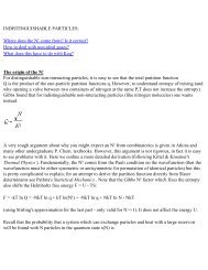
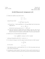
Barefoot empiricism sometimes leads us to non-linearity, too. Examination of data, eithera scatter plot or a residual plot, may reveal a non-linear relationship, between Y and X .While we do not know what the right functional form is, we can capture the relationship inthe data by including additional variables that are powers of X, such as X 1=2 , X 2 , X 3 ,aswell as X . In other words, to capture the non-linear relationship, y = g(x), we approximatethe unknown function , g(x), using a polynomial of the values of x.One note of caution. Including powers of independent variables often leads to collinearityamong the righthand side variables. One trick for breaking such collinearity is to deviatethe independent variables from their means before transforming them.Example: Candidate Convergence in Congressional Elections.An important debate in the study of congressional elections concerns how well candidatesrepresent their districts. Two conjectures concern the extent to which candidatesre°ect their districts. First, are candidates responsive to districts? Are candidates in moreliberal districts more liberal? Second, does competitiveness lead to closer representation ofdistrict preferences? In highly competitive districts, are the candidates more \converged"?Huntington posits greater divergence of candidates in competitive areas { a sort of clash ofideas.Ansolabehere, Snyder, and Stewart (2001) analyze data from a survey of congressionalcandidates on their positions on a range of issues during the 1996 election. There are 292districts in which both of the competing candidates ¯lled out the survey. The authors constructeda measure of candidate ideology from these surveys, and then examine the midpointbetween the two candidates (the cutpoint at which a voter would be indi®erent between thecandidates) and the ideological gap between the candidates (the degree of convergence). Tomeasure electoral competitiveness the authors used the average share of vote won by theDemocratic candidate in the prior two presidential elections (1988 and 1992).The Figures show the relationship between Democratic Presidential Vote share and,respectively, candidate midpoints and the ideological gap between competing candidates.41

There is clear evidence of a non-linear relationship explaining the gap between the candidatesThe table presents a series of regressions in which the Midpoint and the Gap are predictedusing quadratic functions of the Democratic Presidential Vote plus an indicator of OpenSeats, which tend to be highly competitive. We consider, separately, a speci¯cation usingthe value of the independent variable and its square and a speci¯cation using the valueof the independent variable deviated from its mean and its square. The last column usesthe absolute value of the deviation of the presidential vote from .5 as an alternative to thequadratic.E®ects of District Partisanship on Candidate PositioningN = 292Dependent VariableMidpointGapIndependent (1) (2) (3) (4) (5)Variable Coe®.(SE) Coe®.(SE) Coe®. (SE) Coe®. (SE) Coe®. (SE)Democratic Presidential -.158 (.369) | -2.657 (.555) | |VoteDemocratic Presidential -.219 (.336) | +2.565 (.506) | |Vote SquaredDem. Pres. Vote | -.377 (.061) | -.092 (.092) |Mean DeviatedDem. Pres. Vote | -.219 (.336) | +2.565 (.506) |Mean Dev. SquaredAbsolute Value of Dem. Pres. | | | | .764 (.128)Vote, Mean Dev.Open Seat .007 (.027) .007 (.027) -.024 (.040) -.024 (.040) -.017 (.039)Constant .649 (.098) .515 (.008) 1.127 (.147) .440 (.012) .406 (.015)Rp 2 .156 .156 .089 .089 .110MSE .109 .109 .164 .164 .162F(p-value) 18.0 (.00) 18.0 (.00) 9.59 (.00) 9.59 (.00) 12.46 (.00)42

1Midpoint Between Candidate Ideological Positions.8.6.4.20.2 .3 .4 .5 .6 .7 .8Average Dem. Presidential Vote Share43

1Ideological Gap Between Candidates.8.6.4.20.2 .3 .4 .5 .6 .7 .8Average Dem. Presidential Vote Share44

Consider, ¯rst, the regressions explaining the midpoint (columns 1 and 2). We expectthat the more liberal the districts are the more to the leftward the candidates will tend. Theideology measure is oriented such that higher values are more conservative positions. Figure1 shows a strong relationship consistent with the argument.Column (1) presents the estimates when we naively include Presidential vote and Presidentialvote squared. This is a good example of what collinearity looks like. The F-testshows that the regression is \signi¯cant" { i.e., not all of the coe±cients are 0. But, neitherthe coe±cient on Presidential Vote or Presidential Vote Squared are sign¯cant. Tell-talecollinearity. A trick for breaking the collinearity in this case is by deviating X from its mean.Doing so, we ¯nd a signi¯cant e®ect on the linear coe±cient, but the quadratic coe±cientdoesn't change. There is only really one free coe±cient here, and it looks to be linear.The coe±cients in a polynomial regression measure the partial derivatives of the unknownfunction evaluated at the mean of X. Taylor's approximation leads us immediatelyto this interpretation of the coe±cients for polynomial models. Recall from Calculus thatTaylor's Theorem allows us to express any function as a sum of derivatives of that functionevaluated at a speci¯c point. We may choose any degree of approximation to the functionby selecting a speci¯c degree of approximation. A ¯rst-order approximation uses the ¯rstderivatives; a second order approximation uses the second derivatives; and so on. A secondorder approximation of an unknown fuction, then, may be expressed as:1y i ¼ ® + ¯0 x i + x0 iH 0xi;2where" #@f(x)g 0 =@xx=x 0" #@ 2 f (x)H 0 =@x@x0x=x000 x 1® = f (x 0 ) ¡ g 0 + x2¯ = g 0 ¡ H 0 x 0 :0 0H 0 x 045

The coe±cients on the squares and cross-product terms, then, capture the approximatesecond derivative. The coe±cients on the linear values of x equal the gradient, adjusting forthe quadrature around the point at which the data are evaluated (X 0 ). If we deviate all ofthe variables from their means ¯rst, then the coe±cient on X in the polynomial regressioncan be interpreted straightforwardly as the gradient of the (unknown) function at the mean.Example: Candidate Convergence in Congressional Elections, continued.Consider the estimates in column (3). We may analyze these coe±cients to ask several@ybasic questions. What is the marginal rate of change? @DP= ¯1 +2¯2DP. Since DP rangesfrom .2 to .8, the rate of change in the Gap for a change in electoral competition ranges from-1.62 when DP = .2 to +1.42 when DP = .8. At what point does the rate of change equal0 (what is the minimum)? Setting the partial equal to 0 reveals that DP 0 = ¡¯ 1 = :517, so2¯ 2the candidates are most converged near .5. What is the predicted value of the gap at thispoint? 1:127 ¡ 2:657 ¤ :517 + 2:565 ¤ (:517) 2 = :438. At the extremes, the predicted valuesare .64 (when DP = .8) and .70 (when DP = .2).If we must choose among several transformations, such as logarithms, inverses, and polynomials,we typically cannot test which is most appropriate using the Wald test. Davidsonand MacKinnon (1981) propose using the predicted values from one of the non-linear analysisto construct a test. Suppose we have two alternative models: y = X¯ and y = Z°.Consider a compound modely =(1 ¡ ¸)bf X¯ + ¸Z° + ²The J-test is implemented in two steps. First, estimate y = Z° to get Z^ °. Then, include Z^ °^in the regression of y = X¯. The coe±cient on Z^° yields an estimate of ¸. Asymptotically,the t-ratio¸¡0 ^SE(¸tests which model is appropriate.Example: Candidate Convergence in Congressional Elections, continued.An alternative to the quadratic speci¯cation in column (4) is an absolute value speci¯cationin column (5). Notice that the R 2 is slightly better with the absolute value. However,46

owing to collinearity, it is hard to test which model is more appropriate. I ¯rst regress onGap on DP and DP 2 and Open and generated predicted values, call these GapHat. I thenregress Gap on ZG and jDP ¡ :5j and Open. The coe±cient on jDP ¡ :5j is 1.12 with astandard error of .40, so the t-ratio is above the critical value for statistical signi¯cance.The coe±cient on ZG equals -.55 with a standard error of .58. The estimated ¸ is notsigni¯cantly di®erent from 0; hence, we favor the absolute value speci¯cation.47