Lecture (9).pdf - MIT OpenCourseWare

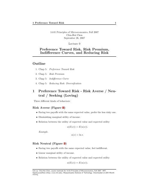
1 Preference Toward Risk114.01 Principles of Microeconomics, Fall 2007Chia-Hui ChenSeptember 26, 2007Lecture 9Preference Toward Risk, Risk Premium,Indifference Curves, and Reducing RiskOutline1. Chap 5: Preference Toward Risk2. Chap 5: Risk Premium3. Chap 5: Indifference Curve4. Chap 5: Reducing Risk: Diversification1 Preference Toward Risk - Risk Averse / Neutral/ Seeking (Loving)Three different kinds of behaviors:Risk Averse (Figure 1)• Facing two payoffs with the same expected value, prefer the less risky one.• Diminishing marginal utility of income.• Relation between the utility of expected value and expected utilityu(E(x)) > E(u(x)).Example.u(x) = lnx.Risk Neutral (Figure 2)• Facing two payoffs with the same expected value, feel indifferent.• Linear marginal utility of income.• Relation between the utility of expected value and expected utilityu(E(x)) = E(u(x)).Cite as: Chia-Hui Chen, course materials for 14.01 Principles of Microeconomics, Fall 2007. MITOpenCourseWare (http://ocw.mit.edu), Massachusetts Institute of Technology. Downloaded on [DD MonthYYYY].

2 Risk Premium232.52u(x)1.510.500 1 2 3 4 5 6 7 8 9 10xFigure 1: The Utility Function of Risk Averse.Example.u(x) = x.Risk Seeking (Figure 3)• Facing two payoffs with the same expected value, prefer the riskier one.• Increasing marginal utility of income.• Relation between the utility of expected value and expected utilityu(E(x)) < E(u(x)).Example.u(x) = x2.2 Risk PremiumRisk premium. The maximum amount of money that a risk-averse personwould pay to avoid taking a risk.Example (Job Choice). Assume that a risk-averse person whose utility functioncorresponds with the curve in Figure 4 has two possible incomes.Cite as: Chia-Hui Chen, course materials for 14.01 Principles of Microeconomics, Fall 2007. MITOpenCourseWare (http://ocw.mit.edu), Massachusetts Institute of Technology. Downloaded on [DD MonthYYYY].

2 Risk Premium398765u(x)432100 1 2 3 4 5 6 7 8 9 10xFigure 2: The Utility Function of Risk Neutral.70605040u(x)30201000 1 2 3 4 5 6 7 8 9 10xFigure 3: The Utility Function of Risk Seeking.Cite as: Chia-Hui Chen, course materials for 14.01 Principles of Microeconomics, Fall 2007. MITOpenCourseWare (http://ocw.mit.edu), Massachusetts Institute of Technology. Downloaded on [DD MonthYYYY].

3 Indifference Curve between Expected Value and StandardDeviation42018161412u(x)10864200 5 10 15 20 25 30xFigure 4: Risk Premium: A Utility Function.• His income I might be 10 with probability 0.5 and 30 with probability 0.5.Then the expected value of income I is:with an expected utility:E(1) = 10 × 0.5 + 30 × 0.5 = 20,E(u(I)) = u(10) × 0.5 + u(30) × 0.5 = 10 × 0.5 + 18 × 0.5 = 14.′ ′• If we offer him a fixed income I , I = 16, then his expected utility is:One can see thatE(u(I′)) = u(16) × 1 = 14 × 1 = 14.′E(u(I)) = E(u(I )).′However, E(I) − E(I ) = 4. This means the person is willing to give up a valueof 4 in exchange for a riskless income. Thus, the risk premium is′Risk Premium = E(I) − E(I ) = 20 − 16 = 4.3 Indifference Curve between Expected Valueand Standard DeviationThe indifference curve we discussed before is about the quantities of two differentgoods, now we consider the indifference curve about expected value and standarddeviation (Figure 5).Cite as: Chia-Hui Chen, course materials for 14.01 Principles of Microeconomics, Fall 2007. MITOpenCourseWare (http://ocw.mit.edu), Massachusetts Institute of Technology. Downloaded on [DD MonthYYYY].

3 Indifference Curve between Expected Value and StandardDeviation513301320131013001290E x12801270126012501240400 500 600 700 800 900 1000σFigure 5: Indifference Curve between Expected Value and Standard Deviation.Probability 0.5 Probability 0.5Job 1 900 1600Job 2 625 2025Table 1: The Income and Probability of Two Jobs.Example (Job choice). Suppose one has the following utility functionu(x) =√ xand two job choices (see Table 1). Calculate expected utilities:E(u(x 1 )) = 0.5 × √ 900 + 0.5 × √ 1600 = 35,E(u(x 2 )) = 0.5 × √ 625 + 0.5 × √ 2025 = 35.Thus, these two jobs give the person the same utility level, i.e. they are on asame indifference curve.In order to plot the indifference curve, we should calculate their expectedvalues and standard deviations.E(x 1 ) = 1250σ(x 1 ) = 494E(x 2 ) = 1325σ(x 2 ) = 990Job 2 has higher expected value of income but it is riskier. (Figure 5)Compare Figure 6 and Figure 7. The former is more risk averse since onemust compensate more for more risk.Cite as: Chia-Hui Chen, course materials for 14.01 Principles of Microeconomics, Fall 2007. MITOpenCourseWare (http://ocw.mit.edu), Massachusetts Institute of Technology. Downloaded on [DD MonthYYYY].

3 Indifference Curve between Expected Value and StandardDeviation69080706050E x4030201000 1 2 3 4 5 6 7 8 9 10σFigure 6: Indifference Curve between Expected Value and Standard Deviation,Larger Slope.2018161412xE10864200 1 2 3 4 5 6 7 8 9 10σFigure 7: Indifference Curve between Expected Value and Standard Deviation,Smaller Slope.Cite as: Chia-Hui Chen, course materials for 14.01 Principles of Microeconomics, Fall 2007. MITOpenCourseWare (http://ocw.mit.edu), Massachusetts Institute of Technology. Downloaded on [DD MonthYYYY].

4 Reducing Risk: Diversification74 Reducing Risk: DiversificationDiversification. Reducing risk by allocating resources to different activitieswhose outcomes are not closely related.Example (Selling air conditioner and heater). Suppose that the weatherhas a probability 0.5 to be hot and 0.5 to be cold. Table 2 shows thecompany’s profit if all its efforts in selling air conditioners (heaters) andthe weather turns out to be hot (cold).Weather Hot ColdAir Conditioner 30,000 12,000Heater 12,000 30,000Table 2: Diversification: Selling Air Conditioners and Heaters.• If one only sells air conditioners or heaters,E(profit) = 21, 000,σ(profit) = 9, 000.• If the company puts half of its efforts in selling air conditioners andhalf of its efforts in selling heaters, then the profit is always 21,000no matter the weather is cold or hot.E(profit) = 21, 000,σ(profit) = 0.Thus we should choose to sell both to reduce risk.Example (Example: Stock versus mutual fund). Mutual fund may havethe same return as stock but much less risk.Example. ”Don’t put all your eggs in one basket.”Cite as: Chia-Hui Chen, course materials for 14.01 Principles of Microeconomics, Fall 2007. MITOpenCourseWare (http://ocw.mit.edu), Massachusetts Institute of Technology. Downloaded on [DD MonthYYYY].