Full Text in PDF - Gnedenko e-Forum

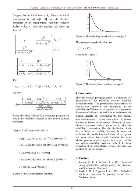
F.GrabskiApplications of semi-Markov processes in reliability - RTA # 3-4, 2007, December - Special IssueSuppose that an initial state is λ0. Hence the initialdistribution is p ( 0) = [1 0]and the Laplacetransform of the unconditional reliability function~ ~is R ( s ) = R 0( s ) . Now the equation (20) takes theform of⎡⎢⎢ 1⎢⎢ α⎢ β 11⎢−⎢⎣( s + + 11 1 ) αβ λFor⎡⎢ 1⎢ s + λ0= ⎢⎢ 1⎢⎢⎣s + λ1−( s + λ0αβ00−α( s + β0+ λ0))( s + ββ11−( s + λ ) ( s + β1βα01α011+ λα11+ λ )α00 )⎤⎥ ⎡R~ ⎤⎥ 0( s)⎢ ⎥⎥ ⎢ ⎥⎥ ⎢ ⎥⎥ ⎢ ⎥⎥ ⎣ R~1( s)⎦⎥⎦⎤⎥⎥⎥⎥⎥⎥⎦α = , α = 3, β = 0.2 , β = 0.5, λ = 0, λ 0.2 ,021 010 1=we have1 0.04 0.04 ⎡ 1 0.125 ⎤− +22 ⎢ −3⎥~ s s(s+0.2) ( s+0.2) 0.2 ( 0.2)( 0.7)0()⎣s+s+s+R s =⎦0.04 0.1251−2 3( s+0.2) ( s+0.7)Using the MATHEMATICA computer program weobtain the reliability function as the inverse Laplacetransform.R(t)= 1.33023exp( −0.0614293t)+ exp( −0.02t)(1.34007⋅10−14+ 9.9198 ⋅10−15t)− 2 exp( −0.843935t)[0.0189459cos(0.171789t)+ 0.00695828sin( 0.171789 t)]− 2 exp( −0.37535t)[0.146168cos(0.224699t)+ 0.128174sin(0.224699 t)]Figure 6 shows the reliability function.10.80.60.40.220 40 60 80 100Figure 6. The reliability function from example 2The corresponding density functionf ( t)= −R'(t)is shown in Figure 70.040.030.020.0120 40 60 80 100Figure 7. The density function from example 28. ConclusionThe semi-Markov processes theory is convenient fordescription of the reliability systems evolutionthrough the time. The probabilistic characteristics ofsemi-Markov processes are interpreted as thereliability coefficients of the systems. If A representsthe subset of failing states and i is an initial state, therandom variable ΘiAdesignating the first passagetime from the state i to the states subset A, denotesthe time to failure of the system. Theorems of semi-Markov processes theory allows us to find thereliability characteristic, like the distribution of thetime to failure, the reliability function, the mean timeto failure, the availability coefficient of the systemand many others. We should remember that semi-Markov process might be applied as a model of thereal system reliability evolution, only if the basicproperties of the semi-Markov process definition aresatisfied by the real system.References[1] Barlow, R. E. & Proshan, F. (1975). Statisticaltheory of reliability and life testing. Holt, Reinhartand Winston Inc. New York.[2] Brodi, S. M. & Pogosian, I. A. (1973). Embeddedstochastic processes in queuing theory. Kiev,Naukova Dumka.- 74 -