A Hybrid Factored Frontier Algorithm for Dynamic Bayesian Networks

More documents

Recommendations

Info

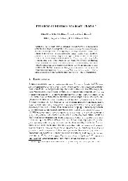
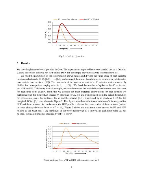
0.30FF Exact Inference Hybrid FF (n^3 Spikes)0.25M t ( E, [0,1) )0.200.150.100.050.001 9 17 25 33 41 49 57 65 73 81 89 97Time pointsFig. 2. M t (E, [0, 1]) for all t5 ResultsWe have implemented our algorithm in C++. The experiments reported here were carried out on a Opteron2.2Ghz Processor. First we ran HFF on the DBN for the simple enzyme catalytic system shown in 1.We fixed the parameters of the system using known values and divided the value space of each variableinto 5 equal intervals [0, 1), [1, 2), . . . , [4, 5] and assumed the initial distributions to be uniformly distributedover certain intervals (see [18]). The time scale of the system was set to be 10 minutes which was evenlydivided into time points ranging over [0, 1, . . . , 100] . We fixed the number of spikes to be 4 3 = 64 andran HFF and FF. This being a small example, we could compute the probability distributions over the statesfor each time point exactly. From this we derived the exact marginal distributions for each species. FFperformed well for the product species P . However for E, ES and S it deviated from the actual distributionfor certain marginals. For instance, for E and the interval [0, 1), it deviated by as much as 0.168 for themarginal M t (E, [0, 1)) as shown in Figure 2. This figure also shows the time evolution of this marginal forHFF and the exact one. As can be seen, the HFF profile is almost the same as that of the exact one (in factthis was already the case for σ = n 2 = 16). Figure 3 shows the maximum error curves for FF and HFFrelative to the exact one; it the maximum of the errors taken over all 5 intervals at each time point. As canbe seen, the maximum error incurred by HFF is lower.Maximum absolute error for E0.180.160.140.120.10.080.060.040.020FF Error Hybrid FF Error1 9 17 25 33 41 49 57 65 73 81 89 97Time pointsFig. 3. Maximum Error of FF and HFF with respect to exact for E7
Fig. 4. EGF-NGF pathwayWe next considered the EGF-NGF pathway in PC12 cells. This cell line is a valuable model systemin neuroscience. Specifically, PC12 cells proliferate in response to EGF stimulation but differentiate intosympathetic neurons in response to NGF. This phenomenon has been intensively studied [9] with a transientactivation of Erk1/2 associated with cell proliferation, while a sustained activity has been linked todifferentiation. The network structure of this pathway shown in figure 4. The ODE model of this pathwayis available in the BioModels database [17]. It consists of 32 differential equations (one for each molecularspecies) and 48 associated rate parameters (estimated from multiple sets of experimental data). Its DBNapproximation was adapted from the one constructed in [15] and details can be found in [14]. We computedthe HFF profiles for various sizes of spikes set. Next we ran FF and compared its profiles with those of HFF.For many of the species FF did quite well. However, 6 species out of 32 exhibited a significant difference,among which were important proteins such as Activated Sos and Activated Erk.Since the DBN consisted of 3200 nodes (32 nodes per time slice; 100 time slices), with each node’svariable assuming 5 possible values, it was not possible to compute the exact probability distributions over5 32 states at each time point. However, to compare the accuracy of FF and HFF (with σ = n 3 = 32768for this DBN), one does not necessarily need the exact distribution. Denoting Mσ t (respectively, MF t F ) themarginal at time t computed by HFF with σ spikes (respectively, FF), the quantity |M t (i, v) − P (Xi t =v)| − |MF t F (i, v) − P (Xt i = v)| does not depend on the exact marginal P (Xt i = v). Rather, it depends onthe marginals (Mσ(i, t v), MF t F(i, v)) and their relative position with respect to the exact marginal.Now, as σ approaches K n (where K = |V |), α approaches 1 and thus the belief states computed by HFFapproach the exact distributions. Hence, we ran HFF with different values of σ -denoted HFF(σ)- rangingfrom HFF(3072) upto HFF(100000) and looked for a pattern. From the relative positions of the curves, andthe high value of α (always bigger than 0.6) for HFF(100000), we infer that the curve for HFF(100000) is onthe same side of FF and HFF(32768) as the exact marginal. Hence, the quantity |M t 32768 (i, v) − M t 100000 | −|M t F F (i, v)−M t 100000 | is a good approximation for |M t 32768 (i, v)−P (Xt i = v)|−|M t F F (i, v)−P (Xt i = v)|.In figure 5 we show for Activated Erk, the computed marginals of the concentration of this protein falling inthe interval [2, 3) for FF as well as HFF(3072), HFF(32768) and HFF(100000).8
Page 6 and 7: The overall error at time t, denote
Page 11: αHFF ( 3072 Spikes) HFF ( 32768 Sp

A Hybrid Factored Frontier Algorithm for Dynamic Bayesian Networks

You also want an ePaper? Increase the reach of your titles

Delete template?

Save as template?