LPC Prediction Error-Analysis of Its Variation with the Position of the ...

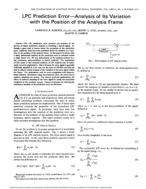
434 IEEE TRANSACTIONS ON ACOUSTICS, SPEECH, AND SIGNAL PROCESSING, VOL. ASSP-25, NO. 5, OCTOBER 1977LPC Prediction Error-Analysis of Its Variationwith the Position of the Analysis Frame.Abstract-The LPC prediction error provides one measure of thesuccess of linear prediction analysis in modeling a speech signal. Althougha great deal is known about the properties of the predictionerror, relatively little has been published about its variation as a functionof the position of the analysis frame. In this paper it is shown thata fairly substantial variation in the prediction error is obtained withina single frame (i.e., 10 ms), independent of the analysis method (i.e.,the. pvariance, autocorrelation, or lattice method). The implicationof this result is that standard methods of LPC analysis may be inadequatefor some applications. This is because the error signal is generallyuniformly sampled at a low rate (on the order of 100 Hz), and this canlead to aliased results because of the variation of the error signal withinthe frame. For applications such as word recognition with frame-toframedistance calculations using the prediction error, the errors due touniform sampling can accrue. For speech synthesis applications, theeffect of uniform sampling of the error signal is a small, but noticeableroughness in the synthetic speech. Various techniques for reducing theintraframe variation of the prediction error are discussed.I. INTRODUCTIONLTHOUGH the class of linear prediction analysis methodsA w [71 are generally well understood, there still remainseveral interesting problems concerning the ways in whichlinear prediction analyses are implemented. One of these openquestions concerns the properties of the normalized LPCprediction-error signal. In particular, there have been fewinvestigations into the variation of the prediction error as afunction of the position of the analysis frame within a singlestationary speech segment. This paper presents results on afairly intensive investigation into this question.11. LPC ERROR SIGNALTo set the problem in its proper perspective it is worthwhilereviewing the LPC analysis model. Fig. 1 shows a blockdiagram of an LPC analysis system. The input speech signal isdenoted as s(n). A pth order linear predictor operates on s(n)to produce the estimate f(n) defined asPi(n) = aks(n - k)k=lwhere the ak are chosen to minimize the mean-squared errorbetween the actual s(n) and the predicted value f(n). Wedefine this difference asPe(n) = s(n) - f(n) = s(n) - aks(n - k). (2)k=lPREDICTORPP oks(n-k)k= 1Fig. 1. Block diagram of LPC analysis system.The ak are thus chosen to minimize the mean-squared errorE, defined asnlE= ez(n)n =nowhere the limits in (3) are appropriately chosen. We shalldenote the sequence of samples of e(n) from n = no to n = nlas the analysis frame. It can readily be shown that an equivalentexpression for the mean-squared error iswhere a. = - 1, and cij is the autocorrelation of the signal,defined as'_ 1cjj =n =nos(n - i) s(n - j).Since the predictor coefficients which minimize E satisfyD2 ajcij = coij= 1(4) is further simplified to the formE=-Pi= 0ajcoj.The normalized LPC error EN is defined by normalizing Eby the signal energy, i.e.,orManuscript received November 16,1976; revised March 22,1977, andMay 9, 1971.The authors are with Bell Laboratories, Murray Hill, NJ 07974.Authorized licensed use limited to: Escuela Superior de Ingeneria Mecanica. Downloaded on November 26, 2009 at 20:19 from IEEE Xplore. Restrictions apply.

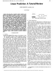
RABINER et al.: LPC PREDICTION ERROR-ITS VARIATION4355949LRR - I Y VOWELM.14 N-200COVARIANCE METHOD4597SAW - AH VOWELM=14 N.200COVARIANCE METHOD-7443 -80130 TIME (SAMPLES) 2i 3 0 TIME ) (SAMPLES 2131622 1 i( bl-1905 0 TIME (SAMPLES) 213104LOG(db)-16220 TIME (SAMPLES) 2i310.6LOG(db)LOG(d b)260 FREOUENCY 05KHZFREPUENCY83ERROR SPECTRUM420 FREOUENCY 5KHZhi511. " I 1 ' ERROR SPECTRUM I0FREPUENCY5KHZ(dlLR - IY VOWELSAW - AH VOWELM = 14 N= 200M= 14 N=X)OAUTOCORRELATION METHODAUTOCORRELATION METHODHAMMING WINDOWHAMMING WINDOW4485 4043(a) (a)- -- -Aw--SIGNAL-49440 TIME (SAMPLES)-70441990 TIME (SAMPLES)137313271-1373 - 1327102 101LOG(db)(c)LOG(db)22 0 FREOUENCY2i5KHZ 0 FREPUENCY 5KHz76 77(3 (dlERROR SPECTRUM .46 u..I0 5KHZ0%HZFREOUENCYFREPUENCYFig. 5. Typical signals and spectra for LPC autocorrelation method fora male speaker.a female speaker.Fig. 3. Typical signals and spectra for LPC autocorrelation method forFigs. 2-5 illustrate some typical analysis frames for two of figure shows the signal samples used in the analysis: partthe well-known methods of LPC analysis; i.e., the covariance (b) shows the resulting error signal (e@)); part (c) shows themethod and the autocorrelation method.' Part (a) of each signal spectrum (as obtained using an FFT analysis) as well as'Results are not presented for the lattice method [ 31 -[7] since theyare almost identical to those obtained for the covariance method.'These figures show all samples used in the analysis. For the covariancemethod the first p samples are not used in computing theprediction residual.Authorized licensed use limited to: Escuela Superior de Ingeneria Mecanica. Downloaded on November 26, 2009 at 20:19 from IEEE Xplore. Restrictions apply.

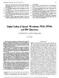
RABINER et ai.: LPC PREDICTION ERROR-ITS VARIATION 4311.4X109LRR-IY VOWELM= 14 N.2002.4X109p y-LRR - I Y VOWELM= 44 N=400ENERGY0 0 50 100 t 50 200 250 300 350 4000 50 100 150 200 250 300 350 400TIME (SAMPLES)TIME (SAMPLES)INORMALIZED ERROR I01 I I I I 1 I I I0 50 100 I50 200 250 300 350 400TIME (SAMPLES)AUTOCORRELATION METHODHAMMING WINDOW0.03001 I I I I 1 I I I0 50 400 150 200 250 300 350 400TIME (SAMPLES 1AUTOCORRELATION METHODHAMMING WINDOWI NORMALIZED 1ERROR0.130 tIC)01 I 1 I I I I I INORMALIZED ERROR0 50 100 150 200 250 300 350 400TI ME (SAMPLES)AUTOCORRELATION METHODRECTANGULAR WINDOWNORMALIZED ERROR0I I I I0 50 100 150 200 250 300 350 400TIME (SAMPLES)Fig. 6. Prediction-error sequemes for 200 samples of speech for threeLPC systems.not linearly predictable. The magnitude of this variation isconsiderably smaller for the analysis using the Hammingwindow (30-percent variation) than for the analysis with therectangular window (about 500-percent variation) due to thetapering of the Hamming window at the ends of the analysiswindow. Another component of the high-frequency variationof the prediction error is related to the position of the analysisframe with respect to pitch pulses, as discussed previously forthe covariance meehod. However, this component of the erroris much less a factor for the autocorrelation analysis than forthe covariance method; especially in the case when a Hammingwindow is used, since new pitch pulses that enter the analysisframe are tapered by the window.01 I I 1 I I I I J0 50 I00 150 200 25Q 300 350 400TIME (SAMPLES)Fig. 7. Prediction-error sequences for N = 400 sample frames.Fig. 7 illustrates the effect of using a longer analysis frame(40 ms) on the prediction error for both the covariancemethod [Fig. 7(b)] and the autocorrelation method using aHamming window [Fig. 7(c)]. Similar effects to those obtainedin Fig. 6 are obtained. However, the magnitude ofthe variation in the prediction error is smaller. For the covariancemethod [Fig. 7(b)] this is true since the frame alwayscontains at least four complete pitch periods, and most of thetime five pitch periods are contained within the frame. Thusthe prediction error is smaller only when the analysis frame ispositioned so that only four error peaks are included withinthe frame. For the autocorrelation method fFig. 7(c)] thecontribution of the first p (14) error terms to the predictionerror is a smaller total percentage of the overall error for a40-ms frame than for a 20-ms frame. Thus again the variationin the high-frequency component of the error is reduced.Fig. 8 illustrates the results obtained for two cases of apitch-synchronous analysis using the covariance method. Fig.8(a) and (b) shows the signal energy and prediction error usinga single period (8.4 ms); whereas, Fig. 8(c) and (d) shows theresults for an analysis frame which is two periods (16.9-ms)long. It is seen in these figures that even though the predictionerror shows long flat regions (i.e., little or no variationwith the analysis-frame position) for both pitch-synchronousanalyses, even slight changes in the pitch period lead tosharp discontinuities in the prediction error. These resultsstrongly suggest that the sensitivity of the prediction error tosmall errors in choosing the pitch period for pitch-synchronousAuthorized licensed use limited to: Escuela Superior de Ingeneria Mecanica. Downloaded on November 26, 2009 at 20:19 from IEEE Xplore. Restrictions apply.

RABINER et ai.: LPC PREDICTION ERROR-ITS VARIATION 439prediction error is the number of whole pitch periods containedwithin the analysis frame.It is important to be able to place some perspective on theimportance and implications of these results. The predictionerror is a measure of the success with which a frame of speechcan be linearly predicted. Thus variations of from 30 to 500percent in the prediction error due to slight shifts of theanalysis-frame position means that the prediction error mustbe carefully interpreted and carefully used in any applicationon which it is based. One such application is the computationof distance proposed by Itakura [lo] based on a ratio ofprediction errors. In this application the quantity D(a, ci),defined asis computed in which Vis a correlation matrix and the termsE2 = dVcit and El =aVat are prediction residuals or normalizedLPC errors based on using the LPC sets li and a. Whatwe have shown is that, depending on the analysis method andthe frame position, variations of E2 on the order of 30-500percent can be obtained. The implications of this variation indefming LPC distance are discussed in Section V.A second case in which variation of the prediction errorwith analysis-frame position may be important is the LPCvocoder. It can be argued that analysis frames with thesmallest prediction error may lead to the best estimates of polecenter frequencies and bandwidths since the peaks in the errorsignal due to the pitch pulses essentially make the analysismore noisy and subject to numerical errors. To test this conjectureLPC synthesis results were obtained using frames withboth the highest and lowest prediction errors and the resultantsynthetic utterances were compared. We discuss these comparisonsin Section VI.Iv. METHODS OF REDUCING THE VARIABILITYOF THE PREDICTION ERRORIn order to reduce the variability in the .LPC prediction errorwith the position of the analysis frame, two distinct preprocessingmethods were investigated. These were as follows.1) Allpass filtering of s(n) to reduce the peakedness of e(n)at the beginning of each pitch period; i.e., to spread out theerror pulse in e@).2) Preemphasizing s(n) by a first-order network to reducethe effects of the high-frequency error in e(n) at the beginningof the frame by making the magnitude of e(n) larger throughoutthe frame.Results of using these two techniques are presented in Figs.10 and 11. Fig. 10 shows the effect on the prediction error ofusing a 24th-order allpass fdter6 [12] to spread out (i.e., phasedisperse) the signal for the covariance method [Fig. lO(b)]and for the autocorrelation method using a Hamming window[Fig. lO(c)]. By contrasting these results with those previouslyshown in Fig. 6, the following effects are noted.6For this implementation the signal was processed by a cascade ofthree of the eight-order allpass filters of [ 91. The detailed nature ofthe allpass filter is not critical. It is important that the effective durationof the impulse response of the allpass filter be large enough tosDread out the excitation over the Ditch Deriod. but not so large so as tosmear the tempord variations of tie preiictor coefficients. -1) For the covariance method the allpass filter effectivelyspreads out the sharp changes in the prediction error signal. Apitch-synchronous variation in the prediction error representinglow-frequency (gradual) changes is now the dominanteffect of varying the position of the analysis frame. In addition,a small noiselike component rides on this low-frequencysignal. The noise is due primarily to the detailed shape of theerror signal from the linear prediction analysis.2) For the autocorrelation method the effect of the allpassfiltering is essentially negligible because the dominant errorterms were shown to be related to the analysis method ratherthati details of the error signal itself. Thus a substantial highfrequencyvariation of the prediction error remains after theallpass fdter is applied.Fig. 11 shows the results obtained for the autocorrelationmethod when a first-order preemphasis network of the formH(2) = 1 - az-1 (14)with a = 0.95 is applied to the speech signal prior to the LPCanalysis. Since the major effect of the preemphasis network isto reduce the spectral variations in the input speech signal,the prediction error increases in value quite significantly overthe values obtained without the preemphasizer. The effectof this increased normalized error is to essentially swamp outthe high-frequency variation in the prediction error due to thefirst p samples since the error signal is uniformly higherthroughout the analysis interval. Thus, as seen in Fig. 1 l(b),the prediction error shows considerably smaller variation withrespect to the position of the analysis frame when the equalizeris used than when it is not used.We did not study the effect of preemphasis for the covariancemethod. The results for the covariance method cannotbe significantly different from those of the autocorrela-tion method. Therefore the reasons previously stated for thereduction in variability of the prediction error for the autocorrelationmethod apply equally well to the covariancemethod; in both cases, the large prediction error resultingfrom the preemphasis of the speech signal wil effectivelyswamp the smaller frame-dependent variations of the predictionerror.The conclusion of this section is that signal conditioningtechniques provide effective methods of reducing the variationin the LPC prediction error with the position of theanalysis frame. It should be noted that the signal conditioningtechniques discussed in this section were independent of thesignal. Signal-dependent methods for reducing the variabilityof the prediction error, such as adjusting the position and sizeof the frame based on the pitch period, can also be applied,but are much morepitch .sensitive to accurate determination ofV. EFFECTS OF PREDICTION-ERROR VARIATIONON AN LE DISTANCE METRICItakura [lo] has proposed a measure of similarity betweenspeech frames with measured LPC sets of a and ci asi.e., the distance between frames is related to the ratio ofprediction residuals or normalized LPC errors. (Other LPCAuthorized licensed use limited to: Escuela Superior de Ingeneria Mecanica. Downloaded on November 26, 2009 at 20:19 from IEEE Xplore. Restrictions apply.

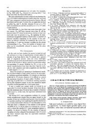
440 IEEE TRANSACTIONS ON ACOUSTICS, SPEECH, AND SIGNAL PROCESSING, VOL. ASSP-25, NO. 5, OCTOBER 19771.4 X109LRR-IY VOWEL -ALLPASSM -14 N.200AUTOCORRELATION METHODHAMMING WINDOWM= 14 N=200LRR-IY VOWEL PRE-EMPHASIZEDO b 50 ,bo 1& 260 2b0 3;o 3 h ATIME (SAMPLES)I I I I I I I 10 50 100 4 5 0 x)o 250 300 350 400TIME (SAMPLES)'2027COVARIANCE METHODNORMALIZED ERROR0.116NORMALIZED ERROR0.0290 50 loo 150 zoo 250 3cil 350 400TIME (SAMPLES)AUTOCORRELATION MEMODHAMMING WINDOW01 I I I 1 I I I J0 50 I0 150 200 250 300 350 400TIME (SAMPLES)Fig. 11. The effects of preemphasis on the prediction-error sequence.and00 50 IO0 150 ZOO a 300 350 400TIME (SAMPLES)Fig. 10.. The effects of allpass filtering on the prediction-error sequence.distance metrics have been proposed by Gray and Markel[I31.) A fundamental implication of the previously givendistance measure is that if a and S are basically from thesame frame, then D(a, 2) should be essentially 0, or El E2.Conver'sely, if a and ri are from dissimilar frames, then D(a, 2)should be large. We have already shown that if a and b representLPC sets obtained from positioning the analysis frame inslightly different positions, then the prediction error can varyby 30 percent or more by itself. This result, by itself, doesnot mean that D(a, 6) wiU vary by 30 percent or more, sinceEl and E2 are not both minimum prediction errors, butinstead El is the error obtained when parameter set a is usedwith the correlation matrix V obtained from parameter set 8.However, this result suggests that significant variations inD(Q, S) might also exist because of variations in the predictionerrorterm E2 due to the position of the analysis frame.To test this hypothesis an LPC analysis was carried out on asample-by-sample basis for a 1.75s utterance. The autocorrelationmethod was used with a 20-ms frame size using a Hammingwindow. The analysis rate was nominally set at 100frames/s. Thus, within each 10-ms frame, 100 LPC analyseswere performed, thereby giving the prediction error at a10000-Hz rate. The positions at which the peak predictionerror and the minimum prediction error occurred were obtained.From the LPC sets corresponding to these two positions(amax and amin) the following quantities were computed:amax Vmin &axDz(amax,amin)= a . . at . (16)mm mm minSince both sets of a's were from ostensibly the same analysisframe, one would theoretically expect Dl and D2 to be closeto 1.0 for all frames. A total of 175 calculations of Dl andDz were made. Fig. 12(a) shows the distribution of theoccurrences of values of Dl, D2 and the combined set ofDl and D2. Of these 175 calculations, Dl exceeded a thresholdof 1.2 a total of 97 times, and Dz exceeded this thresholda total of 85 times; i.e., more than 50 percent of the frameswere classified as dissimilar to shifted versions of the framesusing a 20-percent variation threshold. Additionally, in manycases, the distances exceeded the 20-percent threshold by aconsiderable margin.The previous experiment was repeated on the same sentenceafter it had been preemphasized using the network discussedin the previous section. The results for this case are shown inFig. 12(b). For the 175 frames tested, Dl exceeded thethreshold of 1.2 a total of 34 times, and D2 exceeded thisthreshold a total of 31 times. Of these 67 cases, the majorityoccurred in regions where large signal changes were occurring;Le., in speech transitions, etc., where such behavior is entirelyanticipated. These results indicate that signal preconditioningis a useful technique when a distance measure of the typepreviously described is to be used to compare LPC parametersets.7The implication of the results presented in this section isthat in the worst case when one compares LPC sets obtainedfrom positioning the analysis frame so as to give the maximumand minimum prediction errors, then fairly large distancesbetween such frames can be obtained. Since such frames arephysically the same this result suggests that spuriously largeamin KnaxaLnDl (umin9amax) =amax Laxahax(1 5)7Results are not given for the covariance method, since the LPCdistance of (13) is almost always used with the autocorrelation method.Authorized licensed use limited to: Escuela Superior de Ingeneria Mecanica. Downloaded on November 26, 2009 at 20:19 from IEEE Xplore. Restrictions apply.

Authorized licensed use limited to: Escuela Superior de Ingeneria Mecanica. Downloaded on November 26, 2009 at 20:19 from IEEE Xplore. Restrictions apply.442 IEEE TRANSACTIONS ON ACOUSTICS, SPEECH, AND SIGNAL PROCESSING, VOL. ASSP-25, NO. 5, OCTOBER 1977REFERENCES[ 11 B. S. Atal and S. L. Hanauer, “Speech analysis and synthesis bylinear prediction of the speech wave,” J. Acoust. SOC. Amer.,VO~. 50, pp. 637-655,1971.[2] F. Itakura and S. Saito, “A statistical method for estimation ofspeech spectral density and formant frequencies,” Electron.Commun. Japan, vol. 53-A, pp. 36-43,1970.[3] -, “Digital filtering techniques for speech analysis and synthesis,”in Proc. 7th Int. Congr. Acoustics (Budapest, 1971), Paper25C1.[4] J. D. Markel and A. H. Gray, Linea? Prediction of Speech.Berlin: Springer, 1976.[5] J. Makhoul, “Linear prediction: A tutorial review,” Proc. IEEE,VO~. 63, pp. 561-580, 1975.[ 61 J. Burg, “A new analysis technique for time series data,” NATOAdvanced Study Institute on Signal Processing, Enschede, TheNetherlands, 1968.[ 71 J. Makhoul, “New lattice methods for linear prediction,” in Proc.1976 IEEE Int. Con5 Acoustics, Speech, and Signal Processing,Apr. 1976, pp. 462-465.[8] G. S. Kang, “Application of linear prediction encoding to anarrowband voice digitizer,” Naval Res. Lab. Rep. 7774, Oct.1974.[9] G. S. Kang and D. C. Coulter, “600-bit-per-second voice digitizer(linear predictive formant vocoder),” Naval Res. Lab. Rep. 8043,Nov. 1976.[lo] F. Itakura, “Minimum prediction residual principle applied tospeech recognition,” IEEE Trans. Acoust., Speech, Signal Processing,vol. ASSP-23, pp. 67-72,1975.[ll] S. Chandra and W. C. Lin, “Experimental comparison betweenstationary and nonstationary formulations of linear predictionapplied to speech,” IEEE Trans. Acoust., Speech, Signal Processing,vol. ASSP-22, pp. 403-415, 1974.[12] L. R. Rabiner and R. E. Crochiere, “On the design of all-passsignals with peak amplitude constraints,” Bell Syst. Tech. J., vol.55, pp. 395-407,Apr. 1976.[13] A. H. Gray and J. D. Markel, “Distance measures for speechprocessing,” IEEE Trans. Acoust., Speech, Signal Processing,VO~. ASSP-24, pp. 380-391, Oct. 1976.[14] C. A. McGonegal, L. R. Rabiner, and A. E. Rosenberg, “Asemiautomatic pitch detector (SAPD),” IEEE Trans. Acoust.,Speech, SignalProcessing,vol. ASSP-23, pp. 570-574,Dec. 1975.A Necessary and Sufficient Condition forQuantization Errors to be Uniformand WhiteAbstract-In this paper, a necessary and sufficient condition is givento model the output of a quantizer as an infinite-predsion input and anadditive, uniform, white noise. The statistical properties of the qumtizationerror are studied, and a detailed analysis for Gaussian distributedinputs is given.TI. INTRODUCTIONHE IMPLEMENTATION of filters with digital deviceshaving finite word-length introduces unavoidable quantizationerrors. These effects have been widely studied[6]-[8]. There are three main sources of quantization errorthat can arise: input quantization, coefficient quantization,and quantization in arithmetic operations. Once a model torepresent input quantization error has been developed, modelsto represent the other two types of error can easily be obtained[6]-[8]. Hence, our attention in this paper will be oninput quantization, which occurs in the analog-to-digital conversionprocess.A quantizer can be viewed as a nonlinear mapping from theManuscript received September 17, 1976;revised February 14,1977.This work was supported in part by the National Science Foundationunder Grant ENG74-07800 and in part by the National Institutes ofHealth, Division of Research Resources, under Grant RR00396.A. B. Sripad is with the Department of Systems Science and Mathematics,Washington University, St. Louis, MO 631 30.D. L. Snyder is with the Department of Electrical Engineering and theBiomedical Computer Laboratory, Washington University, St. Louis,MO 63130.domain of continuous-amplitude inputs onto one of a countablenumber of possible output levels. The analysis of errorsintroduced with this mapping can be approached either usingnonlinear deterministic methods [9] or using stochasticmethods [I]-[8]. The later approach is the one we adopt inthis paper.With the stochastic method, the output of the quantizer ismodeled as an infinite-precision input and an additive noise.The additive noise is a random variable whose distribution isnonzero only over an interval equal to the quantization stepsize. Widrow [I] showed that under the condition that theinput random variable has a certain band-limited characteristicfunction, the quantization noise is uniformly distributed; thisis frequently referred to as the “Quantization Theorem”[ 11 -[SI .l The band-limitedness assumption on the inputrandom variable is a sufficient condition that is not satisfieduniversally. In this paper, a weaker sufficient condition whichis also necessary for the Quantization Theorem is given. Thisexpands the class of input distributions for which the uniformnoise model to represent quantization errors can be used withconfidence and is discussed in Section 111.1 More precisely, Widrow established that if the input random variablehas a band-limited characteristic function, then the input distributioncan be recovered from the quantized-output distribution, and thequantization noise density is uniform [l], [2]. Because of its dominantimportance in applications, we are interested in the latter part of thisresult, and refer to it as the “Quantization Theorem’’ for brevity.