A Buffer Stocks Model For Stabilizing Price With

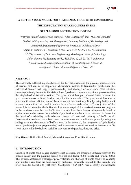
The 20th National Conference of Australian Society for Operations Research & the 5th International Intelligent Logistics System ConferenceA BUFFER STOCK MODEL FOR STABILIZING PRICE WITH CONSIDERINGTHE EXPECTATION STAKEHOLDERS IN THESTAPLE-FOOD DISTRIBUTION SYSTEMWahyudi Sutopo 1 , Senator Nur Bahagia 2 , Andi Cakravastia 3 and TMA. Ari Samadhi 41 Industrial Engineering and Management, Bandung Institute of Technology andIndustrial Engineering Department, University of Sebelas MaretJalan Ir. Sutami 36A, Surakarta 57126, Tell./Fax. 62-271-632110, Indonesia.2, 3, 4 Department of Industrial Engineering, Bandung Institute of TechnologyJalan Ganesa 10, Bandung 40132, Tell./Fax. 62-22-2510680, IndonesiaE-mail: wahyudisutopo@students.itb.ac.id, senator@mail.ti.itb.ac.id,andi@mail.ti.itb.ac.id, samadhi@mail.ti.itb.ac.id 4)ABSTRACTThe extremely different supplies between the harvest season and the planting season are oneof serious problem in the staple-food distribution system. In free-market mechanism, thisextreme difference will trigger price-volatility and shortage of staple-food. This situationcauses opportunity-losses for the stakeholders (producer, consumer, agent and government) inthe staple-food distribution system. The government has got incurred losses because thegovernment cannot achieve food-security for the households. The government has severalprice stabilization policies; one of them is market intervention policy by using buffer stockschemes to stabilize price and to reduce losses for the stakeholders. The objective of thisresearch is to determine the buffer stock schemes required for market-intervention program.In the previous researches, the buffer stock models have been developed separately based onoptimization and econometrics methods. Optimizations methods have been used to determinethe level of availability with schemes consist of time and quantity of buffer stock.Econometrics methods have been used to determine the equilibrium price by using theselling-price and the amount of buffer stock. In this research, the integration of optimizationmodel (multi-objectives programming) and econometrics model are used to develop a bufferstock model with the decision variables that consist of quantity, time, and price.Key Words: Buffer Stock Model, Market-Intervention, Price-Stabilization.1. INTRODUCTIONSupplies of staple-food in agro-industry, such as sugar, are extremely different between theharvest season and the planting season (Reiner and Trcka, 2004, Susila and Sinaga, 2005).This extreme difference will trigger price-volatility and shortage of staple-food. The volatilityand shortage can lead the food-security problems, especially related to the scarcity andprice-hikes for households (ISO, 2005, Mardiyanto, et al, 2005, Susilo, 2006); and related to101.1

The 20th National Conference of Australian Society for Operations Research & the 5th International Intelligent Logistics System Conferencethe crisis of economics and social when the food-security problems are not controlled (Smith,1997, Brennan, 2003). This situation causes opportunity-losses for the stakeholders (producer,consumer, agent/trader, and government) in the staple-food distribution system. Thestakeholders will get losses because the producer is forced to sell staple-food at lowest priceduring the harvest season; the consumer has to deal with the scarcity of staple-food and pricehikes during the planting season; the agent is forced to spend a larger procurement cost andthey lack goods; and the government cannot achieve food security for the households.There are some problems that should be considered in this research, related to the realproblems of staple-food. The amount of production is lower than the amount of consumption.Consequently, import of staple-food is permitted by the government to anticipate marketshortage (Isma’il, 2001, Khudori, 2002, Mardiyanto et al., 2005). The government regulatesthe import mechanism. However, the procurement time is limited during out of harvestseason. The staple-food has high fluctuation in selling price in a year (International SugarOrganization, 2005, Susila and Sinaga, 2005, Susila, 2006). Therefore, market interventionprogram should be conducted by the government to reduce market risks and to maintainfood-security. The government has several price stabilization policies; one of them ismarket-intervention program by using buffer stock schemes (Athanasioa et al, 2008).Buffer stock is a part of inventory as a reserve against short-term shortages and/or todampen excessive fluctuations from supplier (Nur Bahagia, 2006). The buffer stockformulation is identical with safety stock formulation, it is only different in the context ofuncertainty to be anticipated (Tersine, 1994). The government should reduce losses for thestakeholders by storing a certain amount of the staple-food in boom periods so that themarket-price goes up (price-support program); and releases a certain amount of the storedstaple-food in bust periods so that market-prices goes down (price-stabilization program). Inorder to maintain the expectation of stakeholders, the government can apply the buffer stockschemes to maintain the market-price on certain price-band (William and Wright, 2005). Thebuffer stock schemes consist of planning, procurement, inventory, and operation program(Nur Bahagia, 2006).Several authors have addressed to the development of mathematical frameworks toinvestigate the effects of market-intervention program. They are Nguyen (1980), Newbwryand Stiglitz (1982), Jha and Srinivasan (2001), Brennan (2003), Athanasioa et al. (2008)and Sutopo et al. (2008) who have dealt with the stabilization problems by using buffer stock.Nguyen (1980) proposed a simple rule for the buffer stock authorities to stabilize both priceand earnings in every circumstances, not including when market is instable. Newbwry andStiglitz (1982), Jha and Srinivasan (2001) and Brennan (2003) have developed the bufferstock supply model considering price balance at price band policy. These models had beendeveloped to assure welfare both producer and consumer by government’s intervene, butthese models have not considered budget relative with the price-stabilization program yet.However, Jha and Srinivasan (2001) did not consider effectiveness of budgets. Another paper,Athanasioa et al. (2008) presented a Cobweb model with rise of supply according to a certainpiecewise of linear supply function. Furthermore, Sutopo et al. (2008) developed a bufferstock model for stabilizing price of commodity under limited time of supply and continuousconsumption.The previous models cannot dampen excessive fluctuations of supplier side that consist ofamount, price and time simultaneously. In previous researches, the buffer stock models hadbeen developed separately based on optimization methods and econometrics methods.Optimization methods have been used to determine the level of availability with buffer stockschemes consisting of time and amount of buffer stocks. Econometrics methods have beenused to determine the equilibrium price by using the selling price and the amount of buffer101.2

The 20th National Conference of Australian Society for Operations Research & the 5th International Intelligent Logistics System Conferencestocks. We diagnosed a research-question according to the real problems and the mapping ofprevious researches. The objective of this research is to determine the buffer stock schemesrequired for market-intervention program by considering the interests of stakeholders. In thisresearch, the integration of optimization method and econometrics method are used todevelop a buffer stock model for stabilizing price by considering the stakeholder’sexpectation.2. MODELLING FRAMEWORKIn Figure 1, we present the stocks and flows model for stabilizing price throughmarket-intervention program. In this research, we have studied a single commodity producedby the factory and distributed to the consumer through the mediation of agent in free market.The market-prices are determined through 4 periods as follows:(i) the early of harvest season (period t 0 -t 1 ),(ii) the end of harvest season (period t 1 -t 2 ),(iii) the beginning of planting season (period t 2 -t 3 ), and(iv) the end of plantting season (period t 3 -t 4 ).The structural aspect consists of three components of supply-chain entities (producer, agent,and consumer) and a regulator (government) where in this case assumed that each entity hasonly 1 player. The functional aspects consist of the producer-agent-customer relationshipbased on the free market mechanisms; and the producer-government-customer relationshipbased on the intervention of market mechanism.Figure 1.Framework of stocks and flows model at intervention marketFigure1. presents the comparison of transaction between free-market andinterventioned-market. In free-market, the theory of supply and demand states that price itselfis determined by supply and demand forces. At the harvest season, producer sells staple-foodto the agent, and the agent sells them to the consumer. The market-price (producer-agent andagent-consumer) sets off equilibrium process. At the planting season, agent sells staple-foodto the consumer. The market-price (agent-consumer) sets off equilibrium process. Firms withexcess inventories cut prices to try to undersell their competitor.In interventioned-market, the market-price is determined by supply-demand forces andbuffer stock schemes forces. At the harvest season, government intervenes the market with101.3

The 20th National Conference of Australian Society for Operations Research & the 5th International Intelligent Logistics System Conferencethe price-support program when the market-price falls. Price support program is conductedthrough the procurement program from domestic-market. Government purchases thestaple-food in boom periods so that the market-price goes up. At the planting season, thegovernment intervenes the market when the market-price soars with the price-stabilizationprogram. The price-stabilization program is conducted through the market-operation fromstaple-food owned by government. The government releases the staple-food in bush periodsso that the market-price goes down.3. MODEL DEVELOPMENTThe notations of mathematical model is derived with the following (Table 1.):Table 1. Notation of parameters and decision variablesParameters:C : Cost of production by Producer (thousand IDR/kg),PC : Cost of distribution by Agent (thousand IDR/kg),AC : Cost of market operation by Government (thousand IDR/kg),GPAPt: The price producer-agent in t period in free market (thousand IDR/kg),P : The price agent-producer in t period in free market (thousand IDR/kg),ACtPAP*t : The price producer-agent in t period in intervention market (thousand IDR/kg),ACP * : The price agent-producer in t period in intervention market (thousand IDR/kg),tIP : A purchase cost per unit of the staple-food from import (thousand IDR/kg),IRR : Internal Rate of Return as the minimum margin profit-indicator (%),NRR : Normal Rate of Return as the common margin profit-indicator (%),SRR : Speculative Rate of Return as the maximum margin profit-indicator (%),SQt : Total supplies of staple-food from Producer in t period (tons),DQt : Total demand of staple-food from Consumer in t period (tons),Q : Total demand of staple-food from Agent in t period (tons),AtGQ 0 : Amount of staple-food owned by government in the beginning period (tons),h : A holding cost per unit in stock per unit of time (thousand IDR/ton/year),T : Length of time periods, index for time period, t = (1, 4).Decision Variables:MinP : The minimum price-limit (thousand IDR/kg),MaxP : The maximum price-limit (thousand IDR/kg),Q : Amount of staple-food should be purchased from market in t period (tons),OPtQ : Amount of buffer stock should be released to market in t period (tons),ORtIQtAmount of import’s supply in t period (tons),GQt : Amount of staple-food owned by government in t period (tons).First, let consider the simple one-staple-food market model, it is only governed by theDamount of staple-food’s demands in t period ( Q ) from the consumer, the amount oftstaple-food’s production in t period ( Q ) from the producer, the amount of market’s suppliesStAin t period ( Qt ) from the agent, and its price ( P t). Based on partial market equilibriumtheory (a linear model), we translated the simple one-staple-food market model with thefollowing:101.4

The 20th National Conference of Australian Society for Operations Research & the 5th International Intelligent Logistics System ConferenceQQQDtStAtaceCbPt,a, bPdPt,c,dAgPt,e, g0;0;0;(1)(2)(3)Where ( a , c,e)are constants; ( b , d,g)are point price elasticity; then ( a , c,e)and ( b , d,g)should be mutually independent parameters.The objective of development proposed-model is to determine intruments ofMarket-intervention program for giving maximal benefit to the producer (P) and theconsumer (C), and also for giving minimal loss/expenditure to the agent (A) and thegovernment (G). Total benefit or total losses of market-intervention program can becalculated pursuant to total difference between total revenue and total cost at Free Marketwith Intervention Market for each stakelhoder. The description of earnings or expenditure ineach stakeholder is presented at Table 2.Table 2. The description of earnings or expenditure in each stakeholderComponent Free Market (FM) Intervention Market (IM)(P) Total revenue The multiplication of total - The amount of staple-food bought by thesupply from the producerat the selling-price ofgovernment multiplied by the minimumprice-limit.producer-agent. - The amount of staple-food sold to markets at theprice of producer-agent.Total production The total production cost is obtained as the production cost per unit of item(C)costTotalconsumptioncostmultiplied by the quantity of production.The total demand ofconsumer multipliedby selling-price ofagent-consumer.(A) Total revenue The multiplication oftotal supply toconsumer at theselling-price ofagent-consumer.Totalprocurement cost producer-agent.Total distributioncostTotal inventory(G)costTotalprocurement costTotal distributioncostTotal inventorycost- Period t1-t2: the total demand of consumer multipliedby selling-price of agent-consumer.- Period t3-t4: consumer bought the amount ofstaple-food at the maximum price-limit whenmarket-operation controlled by the government, andthe remain one bought at selling-price ofagent-consumer.The total sales is calculated by total consumer’s demandminus the amount of buffer stock when market-operationdone. The revenue is obtained as the selling-price ofagent-consumer multiplied by the Total sales.The amount of staple-food bought from the producer at selling-price ofThe total distribution cost is obtained as the distribution cost per unit of itemmultiplied by total demand of staple-food from the consumer.The total inventory cost is obtained as a holding cost per unit in stock per unit oftime multiplied by total of average inventory in a year.- - The amount of staple-food bought by the governmentfrom the producer at the minimum price-limit.- The amount of staple-food bought by the governmentfrom import at a purchase cost per unit of thestaple-food from import.- The total distribution cost is obtained as cost of marketoperation by the government multiplied by amount ofbuffer stock should be released to market.- The total inventory cost is obtained as a holding cost perunit in stock per unit of time multiplied by total ofaverage the government’s inventory in a year.101.5

The 20th National Conference of Australian Society for Operations Research & the 5th International Intelligent Logistics System ConferenceTotal revenue - The multiplication of amount of buffer stock should bereleased to market at the maximum price-limit.Totalintervention cost- The total intervention cost is obtained as total revenueminus the procurement cost, the distribution cost and theinventory cost.We proposed buffer stocks schemes that consist of 6DVs as instruments for marketinterventionprogram. According to the description either expenses or earning in eachstakeholder shown in Table 2., we can formulate the objective function for each stakeholder.The objective function of proposed-model for the producer is to maximize difference totalprofit betwen IM and FM; and for the consumer is to maximize difference total expenditurebetween IM and FM. The objective function of proposed-model for the agent is tominimize difference total expenditure betwen IM and FM; and for the government is tominimize difference total expenditure between IM and FM. Translated into mathematicalstatements, the total benefit or total cost for producer, consumer, agent and government canbe written as:2Min *PA S OP 2(4)TB P (P QOP) (Q Q ) PPAQSt t t t t tt 1t 1422AC D*PA S OPQ (PMin QOP) P (Q Q ) PPA(5)TB C PQ4[ Pt 1tt 14 D[ PACtQtt 1*ACt( QDtttQORt12 SPPAtQtt 12) Pt 1PAtt4CDAQ tt 1(QStQOPt)tt4h AQt]t 144CDA(Q tt 1ttt 1TC A (6)4 hQOR(QAt) tt 142 OP 4 I 4 OR 4 h G 4max OR (7)TC G PminQItP QtCGQtQtP Q4tt 1t 3 t 3t 1 t 3In this paper, a buffer stock model considers four expectation of stakeholders. Theperformance criterion of the model is to maximize the benefit of both the producer and theconsumer and to minimize the total expenditure of the agent and the government. Theformulation a multi-objectives programming model is as follows:Objective (1):Objective (2):Max.Min.TBTCPATBTCGCAll constraints are classical like the market-price rules, the formulation of stakeholder’sexpectation, the requirement of buffer stock and market clearing of dynamic equilibrium. Themodel is subject to:PA a cA S D(9)Pt[( ) ( Qt1QtQt)]b dAC a e A(10)Pt( ) Qtb g* PA a c A S D(11)P [( ) (OPtQt1QtQtQt)]b d* AC a eA(12)P [( ) (OPtQtQt)]b g* PA MinVT P , P ) VT , (1,2)(13)1(t2tStQOPt)](8)101.6

The 20th National Conference of Australian Society for Operations Research & the 5th International Intelligent Logistics System ConferenceVT (1+ IRR )(14)1C PPAVT2((Pt+ CA) x (1 IRN) - CA)(15)VT ( P* AC, PMax) VT , t3 t4(3,4)(16)VT (PPAC )( 1+ IRR )3 t P(17)VT 4(PPAC )(1t AIRS)(18)44A S OP ORD( Q Q Q Q ) Q , (1,4)(19)t 1 t t tttt 1t 3G OPQt1Qt0, t (1,2)G OR IQt1QtQt0, tQQPStAtMinQQAtORtQOPtQDt, tQDt,t(3,4)(3,4)(1,2)(20)(21)(22)(23)Max OP OR I G, P , Q , Q , Q , Q 0, t T(24)ttttObjective function (8) corresponds to function of multi-objectives in equation (4) until(7), aims to maximize the benefit of both producer and consumer, and to minimize the totallossses or expenditure of agent and government. In free-market, we proposed a market modelwith inventory to determine the selling-price producer-agent and the selling-priceagent-consumer, equations (9) and (10). In intervention-market, we modify a marketmodel with inventory minus the amount of staple-food bought by the government, equations(11) and (12). Where denotes the stock-induced-price adjusment coefficient.We introduce constraints (13), (14) and (15) to ensure that the price-equilibrium fulfilledthe expectation of the producer and the agent at price-support program. The producer’sexpectation is protected from distortion of selling-price as impact of excess supply; and theagent’s expectation is protected from buying-price that costly as the impact of price-floorregulated by the government. We have to ensure the expectation of the agent and theconsumer at price-stabilization program in each period by considering the constrains (16),(17) and (18). The agent’s expectation is protected from fall of selling-price as impact ofceiling-price regulated by the government; and the consumer’s expectation is the availabilityof staple-food at rational selling-price for consumer. The government has to ensure themarket-intervention program could fulfil the demand in each period, constraint (19). We haveto ensure that the buffer stock schemes are adequate to hold the market-interventionprogram in each period by considering the constrains (20) and (21). Finally, we have toensure the supply of staple-food are adequate the demand in each period and to ensure thatall decision variables cannot be negative by considering the constraints (22), (23) and (24).The optimal solution can be obtained by solving the pre-emptive of the multi-objectivesprogramming above. We provide an algorithm to solve the problem illustrated above. Thecomputation technique follows this algorithm:(i) calculate initial price for each supply-availability-demand function, equation (1) until(ii)(7),input model equation (8) until (24) to determine decision variables into GP-ILP softwarei.e. WinQSB, and(iii) calculate objective function by using WinQSB software and determine eachstakeholders objectives.101.7

The 20th National Conference of Australian Society for Operations Research & the 5th International Intelligent Logistics System Conference4. NUMERICAL EXAMPLES AND ANALYSISIn this section, we present numerical examples and analyse them to evaluate the totalstakeholder’s benefit. We consider a set of hypothetic-parameters reflecting one-staple-foodmarket model. It is only governed by the amount of staple-food’s demand, staple-food’sproduction, market’s supplies, and its price. The parameters used for the computationalexample is presented in Table 3. A computational result under a set of price elasticity ofsupply is given as numerical example.Table 3. Parameters of supply-availability-demand (in Units)Parameter a b c d e g hValue 32.0 0.17 167.0 4.8 0.1 0.45 0.1 2.0Parameter C A C G C P P I IRR (%) NRR (%) SRR(%)Value 2.0 4.0 34.0 40.0 5.0 10.0 25.0First, we processed on determining the DVs by using Parameters in Table 3. Weprocessed on determining the decision variables by using GP-ILP software. Computationalresults are shown in Table 4.Table 4. A computational of decision variablesDVsMinPMaxPOPQ tORQ tIQtGQ tPeriod t 1 -t 2 t 3 -t 4 t 1 t 2 t 3 t 4 t 3 t 4 t 1 t 2 t 3 t 4Value 35.7 45.6 0.0 21.6 21.6 21.6 21.6 21.6 0.0 21.6 21.6 21.6The proposed-model has estimated improving the selling-price producer-agent anddegrading the selling-price agent-consumer. The mechanism of improving/degrading isexplained by a market model with inventory. A comparative analysis of price-equilibriumbetween FM and IM is depicted in Table 5.Table 5. A comparative analysis of price-equilibrium between FM and IMPAP t*PAP tACP t*ACP tt 0 t 1 t 2 t 3 t 440.04 36.54 33.5440.04 36.54 35.7051.77 48.27 45.27 47.77 50.2751.77 48.27 47.43 45.61 48.11Based on Table 5, we provide rise or fall of price between free market and interventionmarket. The government conducts the price support program through the procurementprogram from domestic-market at period t 2 , so that the market-price goes up. At the plantingseason [t 3 -t 4 ], the government conducts market-operation through release buffer-stock, so thatthe market-price goes down.101.8

The 20th National Conference of Australian Society for Operations Research & the 5th International Intelligent Logistics System ConferenceTable 6. A comparative analysis between FM and IMStakholder Expectation Notation FM IM Loss/Benefit(Mil. IDR) (Mil. IDR) (Mil. IDR)(P) Total RevenueP( TR ) 3,123.62 3,242.42Production CostP( TC ) 3,060.00 3,060.00Margin(%)Profit 63.62 182.42 118.79 ( 186.72 )(C) Consumption CostC( TC ) 4,789.92 4,681.74 108.18 ( 2.26 )(A) Total RevenueA( TR ) 4,789.92 2,711.39Procurement CostA( TC P) 3,123.62 2,471.30Distribution CostA( TC D) 200.00 113.60Inventory CostA( TC I) 77.50 79.20Profit 1,388.80 47.29 1,341.51 ( 96.59 )(G) Procurement CostG( TC P)2,499.12Distribution CostG( TC D)172.80Inventory CostG( TC I)32.40Total RevenueG( TR )1,970.35Intervention CostG( TC )733.97 ( 15.32 )**)Total Intervention Cost / Total Consumption CostBased on Table 6., the market-intervention program has significantly effect to reduce risksof both the producer and the consumer. We process on determining the stakeholder’sexpectation based on Table 4 and Table 5 for Free-Market and Intervention-Market. Theloss/benefit is obtained as calculation of the difference between total revenue and total cost atFree-Market and intervened-market for each Stakeholder. For a set of hypothetic-parametersgiven, it can be noted that each of total benefit for the producer and the consumer inloss/benefit ratio are 186.72% and 2.26%, respectively. Total cost for the government and theagent in loss/benefit ratio are 15.32% and 96.59%, respectively. For price elasticity given, theproducer obtains the benefit bigger than consumer. Furthermore, the agent obtains thecost/loss bigger than the government.5. CONCLUSIONThis paper provides a buffer stock model for stabilizing price with considering thestakeholders’ expectation in the staple-food distribution system. The proposed-model has asignificant effect to enhance the benefit for both the producer and the consumer under theminimum cost/losses for agent and government. The proposed-model is developed based onthe integration of optimization model (multi-objectives programming) and econometricsmodel (a price-equilibrium model with inventory). A proposed-model is able to obtain thebuffer stock program that its decision variables consist of the quantity, time, and price. Therevenue of price stabilization is intended to induce an equivalent reduction in the fluctuationsof total market revenue. Moreover, the producer gets bigger benefit than the consumer does,and the agent gets bigger cost/losses than the government does.This paper has a certain limitation that should be overcome in order to provide a deepanalysis on the function of a dynamic buffer stock. The ongoing research is dedicated toinclude more realistic price stabilization policy using parameters that appropriate toIndonesian sugar market. Then, further research will focus on other characteristics ofintervention problems, including the effects of multi-player of producer, consumer and agent.ACKNOWLEDGEMENTSThis paper is an initial model of the project-research for stabilizing price of staple-food inIndonesia-Market. The previous results were presented at the 9 th Asia Pacific Industrial101.9

The 20th National Conference of Australian Society for Operations Research & the 5th International Intelligent Logistics System ConferenceEngineering and Management Systems (APIEMS) International Conference inDecember 2008. The authors have benefited from the comments and suggestions of theparticipants at the conference. The authors want to grateful thank to the Directorate General ofHigher Education (DGHE), Ministry of National Education in HIBAH BERSAING ProgramFY 2009 for the support to this research.REFERENCESAthanasioua, G., Karafyllisb, I., and Kotsiosa, S. (2008), Price stabilization using bufferstocks, Journal of Economic Dynamics and Control, 32, pp. 1212-1235.Brennan, D. (2003), Price dynamics in the Bangladesh rice market: implications for publicintervention, Agricultural Economics, 29, pp. 15–25.International Sugar Organization (2005), An International Survey of Sugar Crop Yields andPrices Paid for Sugar Cane and Beet. Market Evaluation Consumption and StatisticsCommittee Report. MECAS, Vol. 05.Isma’il, N.M. (2001), Improvement of Industry Competitiveness National Sugar as Step to FreeCompetition, Institute for Science and Technology Studies Journal, II, pp. 3-14.Jha, S. and Srinivasan, P.V. (2001), Food inventory policies under liberalized trade,International Journal Production Economics, 71, pp. 21-29.Khudori (2002), Restructuring Industrial of National Sugar, Usahawan, No. 03 Th XXXI, pp.3-6, (Published in Indonesia).Labys, W.C. (1980), Survey of Latest Development-Commodity Price Stabilization models:A review and Appraisal, Journal of Policy Modeling, 2 (1), pp. 121-126.Mardiyanto, S., Simatupang, P., Hadi, P.U., Malian, H. and Susmiadi, A. (2005), Roadmap andDevelopment Policy of Industry National Sugar, Forum Penelitian Agro Ekonomi, Vol. 23, No.1,19-37, (Published in Indonesian).Nguyen, D.T. (1980), Partial Price Stabilization and Export Earning Instability, OxfordEconomic Papers, Vol. 32, No. 2, pp. 340-352.Newbery, M.G.D., and Stiglitz, E. J. (1982), Optimal Commodity Stock-Piling Rules, OxfordEconomic Papers, Vol. 34, No. 3, pp. 403-427.Nur Bahagia, S. (2006), Inventory System, 1 st Ed. Penerbit ITB, Bandung, Indonesia. (Publishedin Indonesian).Reiner, G. and Trcka, M. (2004), Customized supply chain design: Problems and alternativesfor a production company in the food industry: A simulation based analysis, InternationalJournal Production Economics, 89, pp. 217–229.Smith, L. (1997), Price Stabilization, Liberalization, and Food Security Conflicts andResolution?, Food Policy, (22), pp. 379-392.Susila, W.R, and Sinaga, B. M. (2005), Analysis Policy of National Sugar Industry, Jurnal AgroEkonomi, Vol. 23, No. 1, pp. 30-53, (Published in Indonesian).Susilo W.R. (2006), High Price Sugar: Had Appropriately, Lembaga Riset Perkebunan Indonesia(LRPI), IT Publications. www. ipard. com. [Accessed April 2007].Sutopo, W., Nur Bahagia, S., Cakravastia, A. and Arisamadhi, TMA. (2008), A Buffer stockModelto Stabilizing Price of Commodity under Limited Time of Supply and Continuous Consumption,Proceedings of The 9 th Asia Pacific Industrial Engineering and Management Systems Conference(APIEMS), pp. 321-329, Bali, Indonesia, December 3 - 5, 2008.Tersine, R.J. (1994), Principle of Inventory Materials Management, Fourth Edition,Prentice-Hall International, Inc., New Jersey, USA.Williams, J.C. and Wright, B.D. (2005), Storage and Commodity Markets, Cambridge UniversityPress, Cambridge, UK.101.10