Masters Thesis - TU Delft

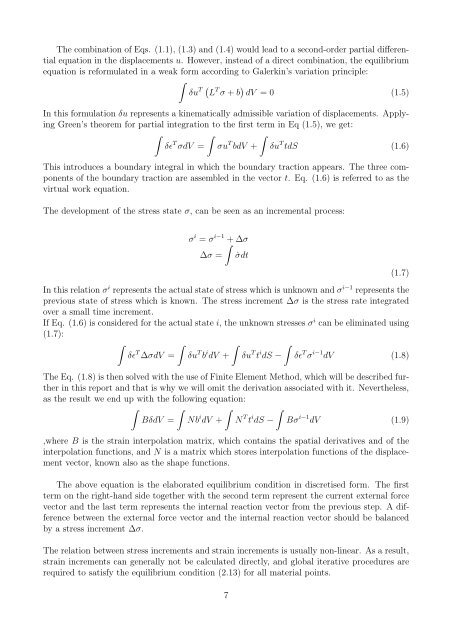
The combination of Eqs. (1.1), (1.3) and (1.4) would lead to a second-order partial differentialequation in the displacements u. However, instead of a direct combination, the equilibriumequation is reformulated in a weak form according to Galerkin’s variation principle:∫δu T ( L T σ +b ) dV = 0 (1.5)In this formulation δu represents a kinematically admissible variation of displacements. ApplyingGreen’s theorem for partial integration to the first term in Eq (1.5), we get:∫ ∫ ∫δǫ T σdV = σu T bdV + δu T tdS (1.6)This introduces a boundary integral in which the boundary traction appears. The three componentsof the boundary traction are assembled in the vector t. Eq. (1.6) is referred to as thevirtual work equation.The development of the stress state σ, can be seen as an incremental process:σ i = σ i−1 ∫+∆σ∆σ = ˙σdtIn this relation σ i represents the actual state of stress which is unknown and σ i−1 represents theprevious state of stress which is known. The stress increment ∆σ is the stress rate integratedover a small time increment.If Eq. (1.6) is considered for the actual state i, the unknown stresses σ i can be eliminated using(1.7):∫ ∫ ∫ ∫δǫ T ∆σdV = δu T b i dV + δu T t i dS − δǫ T σ i−1 dV (1.8)The Eq. (1.8) is then solved with the use of Finite Element Method, which will be described furtherin this report and that is why we will omit the derivation associated with it. Nevertheless,as the result we end up with the following equation:∫ ∫ ∫ ∫BδdV = Nb i dV + N T t i dS − Bσ i−1 dV (1.9),where B is the strain interpolation matrix, which contains the spatial derivatives and of theinterpolation functions, and N is a matrix which stores interpolation functions of the displacementvector, known also as the shape functions.The above equation is the elaborated equilibrium condition in discretised form. The firstterm on the right-hand side together with the second term represent the current external forcevector and the last term represents the internal reaction vector from the previous step. A differencebetween the external force vector and the internal reaction vector should be balancedby a stress increment ∆σ.The relation between stress increments and strain increments is usually non-linear. As a result,strain increments can generally not be calculated directly, and global iterative procedures arerequired to satisfy the equilibrium condition (2.13) for all material points.7(1.7)