Three-Way Independent Samples ANOVA with SAS - Ecu

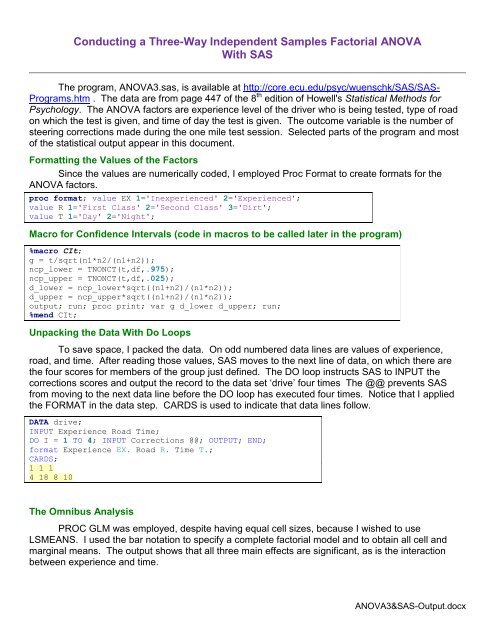
Conducting a Three-Way Independent Samples Factorial ANOVAWith SASThe program, ANOVA3.sas, is available at http://core.ecu.edu/psyc/wuenschk/SAS/SAS-Programs.htm . The data are from page 447 of the 8 th edition of Howell's Statistical Methods forPsychology. The ANOVA factors are experience level of the driver who is being tested, type of roadon which the test is given, and time of day the test is given. The outcome variable is the number ofsteering corrections made during the one mile test session. Selected parts of the program and mostof the statistical output appear in this document.Formatting the Values of the FactorsSince the values are numerically coded, I employed Proc Format to create formats for theANOVA factors.proc format; value EX 1='Inexperienced' 2='Experienced';value R 1='First Class' 2='Second Class' 3='Dirt';value T 1='Day' 2='Night';Macro for Confidence Intervals (code in macros to be called later in the program)%macro CIt;g = t/sqrt(n1*n2/(n1+n2));ncp_lower = TNONCT(t,df,.975);ncp_upper = TNONCT(t,df,.025);d_lower = ncp_lower*sqrt((n1+n2)/(n1*n2));d_upper = ncp_upper*sqrt((n1+n2)/(n1*n2));output; run; proc print; var g d_lower d_upper; run;%mend CIt;Unpacking the Data With Do LoopsTo save space, I packed the data. On odd numbered data lines are values of experience,road, and time. After reading those values, SAS moves to the next line of data, on which there arethe four scores for members of the group just defined. The DO loop instructs SAS to INPUT thecorrections scores and output the record to the data set ‘drive’ four times The @@ prevents SASfrom moving to the next data line before the DO loop has executed four times. Notice that I appliedthe FORMAT in the data step. CARDS is used to indicate that data lines follow.DATA drive;INPUT Experience Road Time;DO I = 1 TO 4; INPUT Corrections @@; OUTPUT; END;format Experience EX. Road R. Time T.;CARDS;1 1 14 18 8 10The Omnibus AnalysisPROC GLM was employed, despite having equal cell sizes, because I wished to useLSMEANS. I used the bar notation to specify a complete factorial model and to obtain all cell andmarginal means. The output shows that all three main effects are significant, as is the interactionbetween experience and time.ANOVA3&SAS-Output.docx

Page 2PROC GLM; CLASS Experience Road Time;MODEL Corrections = Experience|Road|Time / EFFECTSIZE alpha=0.1 ss1;MEANS Experience|Road|Time;LSMEANS Experience*Time / slice = Time;Title 'Omnibus ANOVA and Simple Effects of Experience at Each Level of Time, PooledError'; run;I think that it is appropriate to interpret main effects of factors that are involved in a significant,monotonic interaction, so I have done so here. From the marginal means that are given, it isapparent that inexperienced drivers made significantly more steering corrections than didexperienced drivers, and that steering corrections were significantly more frequent with nocturnaldriving that with diurnal driving. Although I have not done so, one might wish to conduct pairwisecomparisons (Fisher's procedure) among the marginal means for type of road. I think the pattern ispretty clear without additional analysis: Corrections are less frequent on better roads.------------------------------------------------------------------------------------------------Omnibus ANOVA and Simple Effects of Experience at Each Level of Time, Pooled ErrorThe GLM ProcedureClass Level InformationClass Levels ValuesExperience 2 Experienced InexperiencedRoad 3 Dirt First Class Second ClassTime 2 Day Night------------------------------------------------------------------------------------------------Dependent Variable: CorrectionsSum ofSource DF Squares Mean Square F Value Pr > FModel 11 3766.916667 342.446970 12.83 FExperience 1 1302.083333 1302.083333 48.78

Total Variation Accounted ForPage 3SemipartialSemipartial Omega- ConservativeSource Eta-Square Square 90% Confidence LimitsExperience 0.2754 0.2682 0.1045 0.4248Road 0.2150 0.2026 0.0455 0.3542Experience*Road 0.0247 0.0133 0.0000 0.1058Time 0.1943 0.1876 0.0490 0.3474Experience*Time 0.0458 0.0400 0.0000 0.1707Road*Time 0.0106 -0.0007 0.0000 0.0639Experience*Road*Time 0.0309 0.0195 0.0000 0.1193Notice that the Experience x Time effect has a significant F, but the confidence interval for 2 includeszero. The confidence interval for partial 2 excludes zero.Partial Variation Accounted ForPartialPartialOmega-Source Eta-Square Square 90% Confidence LimitsExperience 0.5754 0.4988 0.3261 0.6317Road 0.5141 0.4292 0.2498 0.5776Experience*Road 0.1083 0.0471 0.0000 0.2115Time 0.4888 0.4104 0.2346 0.5609Experience*Time 0.1840 0.1292 0.0244 0.3028Road*Time 0.0495 -0.0027 0.0000 0.1370Experience*Road*Time 0.1319 0.0674 0.0000 0.2372Level of---------Corrections---------Experience N Mean Std DevExperienced 24 12.0833333 5.9191411Inexperienced 24 22.5000000 10.6730054Level of---------Corrections---------Road N Mean Std DevDirt 16 23.1250000 11.4010233First Class 16 11.8750000 6.6017674Second Class 16 16.8750000 8.5936023Level of Level of ---------Corrections---------Experience Road N Mean Std DevExperienced Dirt 8 16.2500000 5.0638777Experienced First Class 8 8.7500000 4.1317585Experienced Second Class 8 11.2500000 6.2507142Inexperienced Dirt 8 30.0000000 12.0356613Inexperienced First Class 8 15.0000000 7.3484692Inexperienced Second Class 8 22.5000000 6.8452277

Level of---------Corrections---------Time N Mean Std DevPage 4Day 24 12.9166667 6.8201534Night 24 21.6666667 10.9133610Level of Level of ---------Corrections---------Experience Time N Mean Std DevExperienced Day 12 9.8333333 5.5240521Experienced Night 12 14.3333333 5.6300062Inexperienced Day 12 16.0000000 6.7823300Inexperienced Night 12 29.0000000 10.0000000Level of Level of ---------Corrections---------Road Time N Mean Std DevDirt Day 8 17.5000000 5.8309519Dirt Night 8 28.7500000 13.1230441First Class Day 8 8.7500000 4.8032727First Class Night 8 15.0000000 6.9282032Second Class Day 8 12.5000000 7.1912645Second Class Night 8 21.2500000 7.9237437------------------------------------------------------------------------------------------------Level of Level of Level of ---------Corrections---------Experience Road Time N Mean Std DevExperienced Dirt Day 4 15.0000000 5.09901951Experienced Dirt Night 4 17.5000000 5.44671155Experienced First Class Day 4 7.5000000 3.87298335Experienced First Class Night 4 10.0000000 4.54606057Experienced Second Class Day 4 7.0000000 4.16333200Experienced Second Class Night 4 15.5000000 5.06622805Inexperienced Dirt Day 4 20.0000000 6.05530071Inexperienced Dirt Night 4 40.0000000 5.88784058Inexperienced First Class Day 4 10.0000000 5.88784058Inexperienced First Class Night 4 20.0000000 4.96655481Inexperienced Second Class Day 4 18.0000000 4.76095229Inexperienced Second Class Night 4 27.0000000 5.71547607Diurnal and Nocturnal Simple Main Effects of ExperienceI elected to approach the significant Experience x Time interaction by testing the diurnal andnocturnal simple main effects of experience. “LSMEANS Experience*Time / slice = Time;” tests thesesimple effects with pooled error.------------------------------------------------------------------------------------------------Least Squares MeansCorrectionsExperience Time LSMEANExperienced Day 9.8333333Experienced Night 14.3333333Inexperienced Day 16.0000000Inexperienced Night 29.0000000

------------------------------------------------------------------------------------------------Experience*Time Effect Sliced by Time for CorrectionsPage 5Sum ofTime DF Squares Mean Square F Value Pr > FDay 1 228.166667 228.166667 8.55 0.0060Night 1 1290.666667 1290.666667 48.35

Simple Effects at Levels of Time, Individual Error.Page 6------------------------------------------- Time=Day -------------------------------------------Dependent Variable: CorrectionsSum ofSource DF Squares Mean Square F Value Pr > FModel 5 612.833333 122.566667 4.83 0.0057Error 18 457.000000 25.388889Corrected Total 23 1069.833333R-Square Coeff Var Root MSE Corrections Mean0.572831 39.00959 5.038739 12.91667Source DF Anova SS Mean Square F Value Pr > FExperience 1 228.1666667 228.1666667 8.99 0.0077Road 2 308.3333333 154.1666667 6.07 0.0097Experience*Road 2 76.3333333 38.1666667 1.50 0.2490Total Variation Accounted ForSemipartialSemipartial Omega- ConservativeSource Eta-Square Square 90% Confidence LimitsExperience 0.2133 0.1851 0.0170 0.4199Road 0.2882 0.2352 0.0195 0.4635Experience*Road 0.0714 0.0233 0.0000 0.2264SSExp | Day 228.16666The eta-squared for Experience during the day is 0. 213. Notice thatSS 1069.8333Total|Daythe denominator is the total sum of squares for the data gathered during the day, excluding thosegathered at night.Partial Variation Accounted ForPartialPartialOmega-Source Eta-Square Square 90% Confidence LimitsExperience 0.3330 0.2497 0.0500 0.4895Road 0.4029 0.2971 0.0640 0.5328Experience*Road 0.1431 0.0403 0.0000 0.3005

------------------------------------------ Time=Night ------------------------------------------Page 7Dependent Variable: CorrectionsSum ofSource DF Squares Mean Square F Value Pr > FModel 5 2235.333333 447.066667 15.97 FExperience 1 1290.666667 1290.666667 46.10

Page 8Simple effects at levels of Time, Individual Error.Plot of Corrections*Experience. Symbol is value of Time.Corrections ‚‚30.0 ˆ‚ N‚‚27.5 ˆ‚‚‚‚25.0 ˆ‚‚‚‚22.5 ˆ‚‚‚‚20.0 ˆ‚‚‚‚17.5 ˆ‚‚‚ D‚15.0 ˆ‚Night DayN‚‚‚12.5 ˆ‚‚‚‚10.0 ˆ D‚ŠƒƒˆƒƒƒƒƒƒƒƒƒƒƒƒƒƒƒƒƒƒƒƒƒƒƒƒƒƒƒƒƒƒƒƒƒƒƒƒƒƒƒƒƒƒƒƒƒƒƒƒƒƒƒƒƒƒˆƒƒInexperiencedExperiencedExperience

Page 9If the Triple Interaction Were SignificantFor pedagogical purposes, let us pretend that the triple interaction is significant. Pretendingsuch, I elected to approach it by testing the diurnal and nocturnal simple interaction betweenexperience and type of road. Since I had earlier included Experience x Road in the model tested bylevels of time of day (individual error terms), we can just look back at that output to get the tests weneed. The output provided by SAS indicates that neither simple interaction is significant, but one ofthem is close. Accordingly, I decided to go ahead and do the extra work to get tests done with thepooled error term from the omnibus analysis, substituting the MSE from the omnibus analysis for theindividual error term reported by SAS. For diurnal driving, the interaction remains not significant,38.16F ( 2, 36) 1.42. Note that I used the PROBF function in SAS to obtain the p for this F, .255.26.69493.16The nocturnal interaction has F ( 2, 36) 3. 49, p = .041.26.694data p;F_Day = 1-PROBF(1.42, 2, 36); F_Night = 1-PROBF(3.49, 2, 36);proc print; Title 'P values for Simple Interactions using pooled error'; run;P values for Simple Interactions using pooled errorObs F_Day F_Night1 0.25493 0.041177Although I obtained the diurnal interaction plot, there is not much to be said about it. Sincethat interaction was not significant, the slopes of the three lines there do not differ from one anothersignificantly, even though the slope with first class roads appears to be distinctly less than that withthe poorer roads.The slopes in the nocturnal interaction plot (22.5, 11.5, 10) differ by more than do those in thediurnal plot (5, 11, 2.5) -- the variance of the slopes is about 47 in the nocturnal plot and about 19 inthe diurnal plot. I included the VAXIS option to control where the tick marks would appear on theordinate. If I had not done so, the two plots would have been scaled differently, and the result wouldbe that the diurnal interaction would appear to be greater than the nocturnal interaction. The nocturnalplot makes it pretty clear that the interaction here is a matter of the effect of experience being muchgreater at night on dirt roads than it is on better roads.

title 'Simple interactions at levels of Time.'; run;proc means data=drive NWAY noprint; class Experience Road; var Corrections;output out=ExR mean= ; by Time;proc plot; plot Corrections*Experience=Road / VAXIS=5 10 15 20 25 30 35 40;by Time; run;Proc gplot;symbol1 interpol=join width=4 value=triangle height=2 color=red;symbol2 interpol=join width=4 value=square height=2 color=green;symbol3 interpol=join width=4 value=circle height=2 color=brown;By Time;plot Corrections*Experience=Road / haxis=1 to 2 by 1;title 'Figure 2. Corrections by Experience, Road, & Time'; run;Simple interactions at levels of Time.Page 10------------------------------------------- Time=Day -------------------------------------------Plot of Corrections*Experience. Symbol is value of Road.40 ˆ‚‚‚‚‚35 ˆ‚‚‚‚‚30 ˆ‚‚Corrections ‚‚‚25 ˆ‚‚‚‚‚20 ˆ D‚‚ S‚‚‚15 ˆDirt Second Class First ClassD‚‚‚‚‚10 ˆ F‚‚‚ F‚ S‚5 ˆŠƒƒˆƒƒƒƒƒƒƒƒƒƒƒƒƒƒƒƒƒƒƒƒƒƒƒƒƒƒƒƒƒƒƒƒƒƒƒƒƒƒƒƒƒƒƒƒƒƒƒƒƒƒƒƒƒƒƒƒˆƒƒInexperiencedExperiencedExperience

Page 12I tested the simple, simple main effects of experience for the three types of road at night byfirst creating a new data set, containing only the nocturnal data, and then testing the effect ofexperience by type of road. As you can see, the effect is significant at each level of the road variable,but is much stronger with the dirt road. I would recommend estimating values of d for each of thesesimple, simple main effects, and obtaining confidence intervals for those estimates, but I have notdone that here.data night; set drive; if Time = 2; proc sort; by Road;proc GLM; class Experience;model Corrections = Experience / EFFECTSIZE alpha=0.1; by Road;title 'Simple, simple main effects of Experience at Road for Time = night.'; run;

Simple, simple main effects of Experience at Road for Time = night.Page 13--------------------------------------- Road=First Class ---------------------------------------The ANOVA ProcedureDependent Variable: CorrectionsSum ofSource DF Squares Mean Square F Value Pr > FModel 1 200.0000000 200.0000000 8.82 0.0249Error 6 136.0000000 22.6666667Corrected Total 7 336.0000000R-Square Coeff Var Root MSE Corrections Mean0.595238 31.73968 4.760952 15.00000-------------------------------------- Road=Second Class ---------------------------------------Sum ofSource DF Squares Mean Square F Value Pr > FModel 1 264.5000000 264.5000000 9.07 0.0237Error 6 175.0000000 29.1666667Corrected Total 7 439.5000000R-Square Coeff Var Root MSE Corrections Mean0.601820 25.41467 5.400617 21.25000------------------------------------------ Road=Dirt -------------------------------------------Sum ofSource DF Squares Mean Square F Value Pr > FModel 1 1012.500000 1012.500000 31.48 0.0014Error 6 193.000000 32.166667Corrected Total 7 1205.500000R-Square Coeff Var Root MSE Corrections Mean0.839900 19.72719 5.671567 28.75000Strength of Effect Estimates: dI prefer estimated d over 2 as a strength of effect estimate, so I have obtained estimated d foreach of the one-df effects that was significant in the omnibus analysis and have also obtained thecorresponding confidence intervals. I also obtained these same statistics for the simple main effects

of experience, day and night.Page 14title 'Get t values for estimating d with confidence interval.'; run;proc ttest data=drive; class experience; var corrections;proc ttest data=drive; class time; var corrections;proc ttest data=drive; class experience; var corrections; by time; run;***********************************************************************;title 'Estimated d for Experience.';run;Data CId; t= 4.18; df = 46; n1 = 24; n2 = 24; %CIt***********************************************************************;title 'Estimated d for Time of Day.';run;Data CId; t= 3.33; df = 46; n1 = 24; n2 = 24; %CIt***********************************************************************;title 'Estimated d for Experience during the Day.';run;Data CId; t= 2.44; df =22; n1 = 12; n2 = 12; %CIt***********************************************************************;title 'Estimated d for Experience at Night.';run;Data CId; t= 4.43; df =22; n1 = 12; n2 = 12; %CItGet t values for estimating d with confidence interval.Experience Method Mean 95% CL Mean Std Dev 95% CL Std DevInexperienced 22.5000 17.9932 27.0068 10.6730 8.2952 14.9717Experienced 12.0833 9.5839 14.5828 5.9191 4.6004 8.3031Diff (1-2) Pooled 10.4167 5.4021 15.4312 8.6299 7.1712 10.8390Method Variances DF t Value Pr > |t|Pooled Equal 46 4.18 0.0001Get t values for estimating d with confidence interval.Time Method Mean 95% CL Mean Std Dev 95% CL Std DevDay 12.9167 10.0368 15.7966 6.8202 5.3007 9.5670Night 21.6667 17.0584 26.2750 10.9134 8.4820 15.3088Diff (1-2) Pooled -8.7500 -14.0377 -3.4623 9.0999 7.5618 11.4293Method Variances DF t Value Pr > |t|Pooled Equal 46 -3.33 0.0017------------------------------------------------------------------------------------------------Simple Main Effects Follow------------------------------------------- Time=Day -------------------------------------------Experience Method Mean 95% CL Mean Std Dev 95% CL Std DevInexperienced 16.0000 11.6907 20.3093 6.7823 4.8046 11.5156Experienced 9.8333 6.3235 13.3431 5.5241 3.9132 9.3792Diff (1-2) Pooled 6.1667 0.9299 11.4035 6.1853 4.7837 8.7543Method Variances DF t Value Pr > |t|Pooled Equal 22 2.44 0.0231

------------------------------------------ Time=Night ------------------------------------------Page 15Experience Method Mean 95% CL Mean Std Dev 95% CL Std DevInexperienced 29.0000 22.6463 35.3537 10.0000 7.0840 16.9788Experienced 14.3333 10.7562 17.9105 5.6300 3.9883 9.5591Diff (1-2) Pooled 14.6667 7.7963 21.5370 8.1147 6.2759 11.4852Method Variances DF t Value Pr > |t|Pooled Equal 22 4.43 0.0002------------------------------------------------------------------------------------------------Estimated d for Experience.Obs g d_lower d_upper1 1.20666 0.58421 1.81803------------------------------------------------------------------------------------------------Estimated d for Time of Day.Obs g d_lower d_upper1 0.96129 0.35787 1.55536------------------------------------------------------------------------------------------------Estimated d for Experience during the Day.Obs g d_lower d_upper1 0.99613 0.13419 1.83814------------------------------------------------------------------------------------------------Estimated d for Experience at Night.Obs g d_lower d_upper1 1.80854 0.83379 2.75463PlotsNotice that I used both Proc Plot and Proc Gplot to produce the plots. The plots produced byGplot can be exported to image files, just select the plot and then click “File,” “Export as Image.”Those produced by Proc Gplot look a lot better than those produced by Proc Plot, but Gplot can beconfusing to use. A good alternative is to use Excel.Presentation of the ResultsAs shown in Table 1, all of the main effects were large and significant. Experienced driversmade significantly fewer errors (M = 12.1) than did inexperienced drivers (M = 22.5), d = 1.207, 95%CI [.584, 1.818]. Errors were most frequent on dirt roads (M = 23.12), intermediate on second classroads (M = 16.88), and least frequent on first class roads (M = 11.88). Errors were significantly morefrequent at night (M = 21.7) than during the day (M = 12.9), d = .961, 95% CI [.358, 1.555].

Page 16Table 1. ANOVA Source Table.Source df F p η 2 CI .90 for η 2Experience 1 48.78 < .001 .275 .104, .425Road 2 19.04 < .001 .215 .046, .354Time 1 34.42 < .001 .194 .049, .347Exp x Road 2 2.19 .12 .025 .000, .106Exp x Time 1 8.12 .007 .046 .000, .171Road x Time 2 0.94 .40 .011 .000 .064E x R x T 2 2.73 .08 .031 .000, .119Error 1 361 MSE = 26.69Among the interactions, only Experience x Time was statistically significant, and it was small inmagnitude when compared to the main effects. Simple effects analysis showed that experienceddrivers made significantly fewer errors than did inexperienced drivers both during the day (M = 9.83,16.00), F(1, 36) = 8.55, p = .006, d = .996, 95% CI [.134, 1.838], and at night (M = 14.33, 29.00) ,F(1, 36) = 48.35, p < .001, d = 1.809, 95% CI [.834, 2.755], with the difference at night greater thanduring the day (see Figure 1).For Even More Fun, Try ….Wow, three-way ANOVA certainly is a lot more fun than one- or two-way ANOVA. Now I wantto do a six-way ANOVA. With how many F tests would I be blessed with six factors? The answer ishere.Karl L. Wuensch, Dept. of Psychology, East Carolina Univ., Greenville, NC, USAFebruary, 2014.SAS Lessons