Mobile-Source Emissions - Center for Environmental Research ...

Transportation Research Record 1842 ■ 91Paper No. 03-4207Mobile-Source EmissionsAnalysis of Spatial Variability in Vehicle Activity Patterns andVehicle Fleet DistributionsCarrie Malcolm, Theodore Younglove, Matthew Barth, and Nicole DavisAccurately estimating mobile-source emissions requires a good understandingof vehicle activity and the characteristics of the on-road vehiclefleet. Spatial variability in vehicle activity patterns and vehicle fleet compositioncan have significant effects on the overall emissions inventory.Simply determining total vehicle miles traveled is insufficient for emissionsinventory calculations from the new-generation models of mobilesourceemissions. Improvements in emissions-control technology overthe past 20 years have led to large decreases in the emissions of light-dutycars and trucks, resulting in large variations in vehicle emissions dependingon model year and technology type. In addition, research indicatesthat the accurate characterization of vehicle activity is necessary in conjunctionwith better spatial resolution of vehicle fleet characteristicsbecause of the differing modal behavior of the vehicles within variousvehicle and technology groups. Vehicle activity and vehicle fleet datawere collected in the South Coast Air Basin in southern California. Vehicleactivity was characterized primarily using a large second-by-secondspeed and acceleration data set collected from probe vehicles operatedwithin the flow of traffic. In addition, three sets of vehicle fleet data werecollected and used for spatial comparison. The results of the analysisshow spatial and temporal differences in vehicle activity patterns andvehicle fleet characteristics; differences in speed and congestion affect thespeed–acceleration profiles as well as associated emissions.University of California–Riverside, College of Engineering, Center for EnvironmentalResearch and Technology, Riverside, CA 92521.Three critical components are used in developing accurate inventoriesof mobile-source emissions: vehicle emissions rates, vehicleactivity patterns, and vehicle fleet distributions. To date, much efforthas been spent on developing accurate real-world vehicle emissionsrates; however, less effort has been applied to correctly identifyingreal-world vehicle activity patterns and vehicle fleet distributions.Vehicle activity has frequently been characterized using averagespeed and vehicle miles traveled (VMT), but advances in the modelingof mobile-source emissions have increased the resolution invehicle activity necessary for using the new models to their full capabilities.In addition to characterization of vehicle activity at greaterresolution, characterization of the vehicle fleet at higher levels of spatialresolution has also been recognized as an important factor for theimprovement of the modeling of mobile-source emissions.Accurate estimation of emissions from on-road sources requiresunderstanding the characteristics of the on-road vehicle fleet. Determiningthe VMT for all vehicles is necessary, but not sufficient.Improvements in emissions-control technology over the past 20 yearshave led to large decreases in the emissions of light-duty automobilesand trucks, resulting in large differences in vehicle emissionsdepending on model year and technology type. Variation inthe on-road fleet composition by time and location can lead to significantdifferences in emissions in both absolute and relative terms,such as the ratio of hydrocarbons (HCs) to nitrogen oxides (NO x ).Previous research at the University of California, Riverside, Collegeof Engineering, Center for Environmental Research and Technology(CE-CERT) indicated that the relatively high proportion of newvehicles found in areas such as national parks results in significantlylower emissions for the national park vehicle fleet compared with atypical urban fleet (1, p. 20).Vehicle fleet characterization has been included at the countylevel in the latest revisions of the EMFAC emissions model (2).Characterization at the zip code level has been included as an optionin the MEASURE model (3) and the Comprehensive Modal EmissionsModel (CMEM; 4). The problems associated with using motorvehicle registration data to develop locally derived vehicle fleets wereaddressed at the 81st Annual Meeting of the Transportation ResearchBoard (5). Furthermore, differences in motor vehicle registrationaddress data and on-road measured license plate data were recentlycharacterized with an estimation of changes in emissions generatedusing the different sources of fleet data (6, p. 19; 7, p. 8).During the summer of 2001, detailed on-road vehicle fleet data(as well as probe vehicle-based activity data, described below) werecollected as part of the Study of Extremely Low Emission Vehicles(SELEV) Program in the South Coast Air Basin (SoCAB), California(6). The SELEV Program at CE-CERT is a multiyear programwith multiple sponsors that has three overall objectives:• To develop, demonstrate, and verify technologies and techniquesfor measuring vehicle emissions at very low levels;• To understand how new-technology vehicles are used in thereal world and measure their emissions; and• To understand the implications of advanced-technology vehiclesfor atmospheric impacts at the micro, meso, and macro scales.In addition to this on-road program of data collection via licenseplates, CE-CERT conducted a random subsample of California’s1998 Department of Motor Vehicles (DMV) registration databasefor the same SoCAB locations. Furthermore, another vehicle fleetstudy was recently completed by CE-CERT on a statewide basis forthe California Air Resources Board (CARB) (7). These three datasources consist of• More than 16,000 vehicles identified by license plate at threeSoCAB cities in the summer of 2001,• A random subsample of more than 70,000 vehicles indexed byregistration zip code, and

92 Paper No. 03-4207 Transportation Research Record 1842• More than 67,000 vehicles were identified by decoding the vehicleidentification numbers (VINs) obtained from data collected inparking lots throughout California in the summer of 2000.License plate capture and subsequent VIN decoding provide detailedvehicle fleet characteristics for determining the vehicle fleet withhigh spatial resolution.In addition to data about the vehicle fleet, a large amount of vehicleactivity data was collected as part of the same SELEV programin 2001. Sites were studied in three SoCAB cities on three differentroadway types (freeway, arterial, and residential). The three citiesselected were Riverside, Yorba Linda, and La Puente in Riverside,Orange, and Los Angeles Counties, respectively (Figure 1). Studentteams collected on-road vehicle activity measurements (i.e., secondby-secondposition, velocity, and acceleration) with an instrumentedvehicle, and general traffic flow data and on-road vehicle licenseplate information with digital video cameras. The teams collecteddata twice during all daylight hours on weekends and weekdays ineach city. Additional details are provided in the methodology section.The primary goal of this vehicle activity study was to characterizethe microscale spatial and temporal variation of vehicle activity andfleet makeup. Data were analyzed using an Autoscope device (8) andVIN-decoding software. The results were compared with existingdatabases and incorporated into a geographical information systemframework for determining link-based emissions inventories. Thelink emissions factors can be generated from CE-CERT’s CMEM (4)when the representative vehicle activity and fleet distribution data areapplied directly to CMEM. In addition to the data mentioned above,macroscale traffic parameters were recorded from the Caltrans PerformanceMeasurement System, coinciding with instrumented vehicledata collection. The generated link emissions factors can be usedin conjunction with the measures of traffic performance to generatereal-time inventories of emissions from mobile sources (9, p. 15).The goal of this paper is to characterize the microscale spatial andtemporal variation of vehicle activity and fleet makeup, with the purposeof improving estimates of real-world vehicle emissions. Thisvehicle activity–fleet distribution data set has been extensively analyzedas a function of location, time of day, and weekday versusweekend.METHODOLOGYOn-Road Vehicle Activity and Vehicle Fleet DataAs part of the SELEV vehicle activity and fleet distribution study,vehicle-driving patterns were collected in three SoCAB cities onresidential, arterial, and freeway routes. A general summary andanalysis of the vehicle activity fieldwork that took place in the summerof 2001 has been published (6). Three primary techniques wereused for data collection:• Second-by-second position and velocity data were recordedusing an instrumented vehicle equipped with Doppler speed sensors,an OBD-II interface, and Global Positioning System instrumentation.• Traffic information was collected using digital video camerasand postprocessed to obtain vehicle class distribution, average trafficspeed, density, and flow rates.• License plate data were captured with a digital video cameraand subsequently analyzed using vehicle registration databases andVIN decoders.Data were collected in Riverside, Yorba Linda, and La Puente(Figure 1). These sites, selected via a rigorous process to ensure theirrepresentativeness of the Los Angeles Basin, included routes in Riverside,Orange, and Los Angeles Counties. Freeway, arterial, and resi-FIGURE 1Site locations in Riverside, Yorba Linda, and La Puente, California.

Malcolm et al. Paper No. 03-4207 93dential roadways were examined at each location. Data were collectedin each city twice for 2 weeks, with 3 days of data collection perweek (two weekdays and one weekend day). Every hour during daylighthours, 20 min of data were collected, rotating among freeways,arterials, and residential streets.Student teams collected on-road measurements of vehicle activitywith an instrumented vehicle; they collected general trafficflow and on-road vehicle license plate data with digital cameras.While one team member collected on-road vehicle activity measurementswith the instrumented vehicle, the other two team membersrecorded general traffic flow and vehicle license plates. Theroute was repeated as many times as time and traffic conditionspermitted.Data were collected between June 25 and Sept. 15, 2001. Theinstrumented vehicle was driven over predetermined routes at eachsite in the three cities. The starting location was rotated, enablingsampling at various locations at different times of the day. Samplingwas conducted for 20 to 30 min at a single location and moved to adifferent location every hour. Three sampling days were completedeach week—alternating Monday, Wednesday, and Saturday withTuesday Friday, and Sunday—for a total of 36 days of testing. Theresulting data set covered all hours of the day for both weekdays andweekends.An Autoscope 2004 unit was set up as a traffic analysis base stationin the research lab. The Autoscope device digitizes and processesimages from a digital video camera to extract traffic parameters suchas number of vehicles and vehicle speed (8). A computer is connectedto the Autoscope; virtual detectors are created on the road image thatemulates an inductive loop. A detection signal is created when a vehiclecrosses a virtual detector. The processor then compiles the data tocreate output files containing information on total volume, volumeby vehicle class, and average speed. The vehicle classes are Class 1(light-duty automobile, less than 25 ft), Class 2 (medium-duty truck,25 to 36 ft), and Class 3 (heavy-duty truck, more than 36 ft), and vehiclelength is calculated from the amount of time a vehicle occupies avirtual detector. To collect the input video stream, a digital video camerawas set up to collect data from all lanes of traffic from at least15 ft above the roadway. At arterial and residential sites, the entireroad was recorded; at freeway sites, only one direction of roadwaywas recorded.A second digital camera was set up along the roadway on a tripodto capture the license plate data of vehicles passing through the datacollectionarea. One lane was captured per day, per site, and a differentlane was captured each day. Still images of the desired frameswere saved, and all identifiable plates were manually entered intoa database, along with the vehicle class. Every minute of traffic atarterial and residential sites was analyzed, and only every third minuteof traffic at freeway sites was collected because of the large volume ofvehicles passing the camera during the taping period. The licenseplate data of each vehicle were run through the registration databaseto obtain make, model, engine, catalyst type, transmission, andhome zip code.On-Road Destination Vehicle Fleet DataThe second source of vehicle fleet data used in this analysis was anon-road vehicle population of light-duty vehicles collected as part ofCARB’s statewide unregistered vehicle project (10, p. 14). The vehicleswere photographed in parking lots throughout the state in thesummer of 2000. License plate data were entered into a database,then correlated with motor vehicle registration data to obtain vehi-cle information. For comparison with the other data sets used inthis analysis, the on-road destination data were restricted to thesites in Los Angeles, Orange, and Riverside Counties. The vehiclesin this analysis are a random sample of the on-road vehicle fleet capturedat destinations throughout the SoCAB. The DMV registrationvehicle fleet data, the on-road vehicle fleet data, and the on-roaddestination data provide slightly different means of comparingvehicle fleets in the study area. Although data collection occurredduring calendar years 2000 and 2001 for the on-road vehicle fleets,the analysis presented in this paper is limited to vehicles with modelyears of 1998 and older because the DMV database available is forcalendar year 1998. CE-CERT is investigating obtaining a morerecent on-site database.RESULTSVehicle Activity from Instrumented VehicleDuring the vehicle activity portion of the study, 540 trips were completedand more than 475,000 s of activity data were recorded. In theanalysis presented in this paper, only freeway activity is considered.With a few exceptions, average weekend speeds (averaged over theentire day) were slightly higher than weekday speeds for the freewaydata at all three locations. The average overall freeway speedwas 58.6 mph (94.3 km/h)—57.1 mph (91.9 km/h) on weekdaysand 60.1 mph (96.7 km/h) on weekends. For all three cities, thewestbound and eastbound freeway traffic patterns differ. As wasexpected, the morning eastbound speeds were the highest, followedby midday speeds, with the slowest speeds on weekday and weekendevenings. The westbound patterns in Riverside are the same asthe eastbound patterns, while Yorba Linda and La Puente weekdaypatterns are the reverse: the morning speeds were slowest and theevening speeds highest. This finding is consistent with commuterpatterns for Yorba Linda and La Puente, where the peak morningcommute is in the westbound direction (for commuters traveling intoOrange and Los Angeles Counties), and the peak evening commuteis in the eastbound direction.Speed–acceleration contour plots were created from the freewaydata for each city to provide an overall summary of the drivingacross the entire period of data collection (Figure 2). Freewaytravel in Riverside tended to be near free flow, while Yorba Lindawas either near free flow or heavily congested. The travel throughLa Puente was more constant, with fewer large acceleration-anddecelerationevents.The data summarized in the location graphs were collected overseveral weeks, including weekdays and weekends. Individual trafficevents can be expected to influence congestion levels; however,the differences apparent in Figure 2 are due primarily to differencesin the predominant vehicle activity patterns for the areas.Although the speed–acceleration distributions are different forthe three locations, the primary factor influencing the differencesin distribution appears to be the level of congestion. Hourly speed–acceleration distributions were created for each city; examples ofchanging traffic behavior are shown in Figure 3. The “×” in eachplot indicates the average speed of that distribution. As averagespeed decreases, the distribution spreads out over a wider range ofspeeds, which is a characteristic of congested conditions. It is interestingto note that the range in speeds (i.e., the distribution spread)is smallest for the most-congested and least-congested traffic conditions,with a much larger range in observed speeds for the midrangeto moderate congestion levels.

94 Paper No. 03-4207 Transportation Research Record 1842(a)(b)FIGURE 2 Speed–acceleration distributions for freeways in (a ) Riverside, (b) Yorba Linda, and(c ) La Puente, California. Frequency indicates the number of occurrences of each speed andacceleration point.(c)To get an idea of emissions associated with these different congestionconditions, each of the example speed distributions in Figure3 was modeled in CMEM (4), calibrated for a Riverside fleet.The resulting emissions factors (in grams per mile) are also shownin Figure 3. As expected, emissions of carbon monoxide (CO 2 ) (asurrogate for fuel use) decrease with speed until levels of congestionincrease, then emissions also increase. Grams-per-mile emissionsof carbon dioxide (CO), HC, and NO x are highest for thehigh-speed, free-flow conditions; lower for the midrange, congestedspeeds; and high again at low, congested speeds. High-speed, freeflowtraffic produced the highest levels of emissions, followed bylow-speed, highly congested traffic. Vehicle behaviors (e.g.,acceleration-and-deceleration events, speed) affect emissionsrates. In low-speed, highly congested traffic, vehicles either pacetogether at similar low speeds (as in La Puente) or have multipleacceleration-and-deceleration events (as in Yorba Linda).Vehicle Activity from AutoscopeThe videotapes collected at each site were processed as described inthe methodology section, and the resulting output files were sum-marized. The Autoscope calculated vehicle speed and vehicle countby classification. The videotapes for the freeway sites captured traffictraveling in the westbound direction for all three cities and in bothdirections for the arterial and residential sites. Figure 4 is a diurnalplot of average freeway volume for weekdays and weekends in eachcity. Yorba Linda tended to have the highest vehicle volumes, especiallyduring weekday evenings and weekend afternoons; vehiclevolumes were lowest in La Puente. These data vary by time of dayand between weekday and weekend. In general, morning volume islower than evening volume.The processor also places vehicle counts into vehicle-type bins ofautomobile, truck, and heavy-duty truck. The average percentage ofheavy-duty trucks in the freeway vehicle fleet is 2.35% in Riverside,7.45% in Yorba Linda, and 6.17% in La Puente.Vehicle Fleet MixVehicle model year was used to identify differences in the vehiclefleet among the three sites. Other factors such as automobile-totruckratios and manufacturer proportions could be used to deter-

Malcolm et al. Paper No. 03-4207 95(a)(b)(c)(d)(e)FIGURE 3 Velocity–acceleration distributions for different levels of freeway congestion. Average trafficspeed is indicated by an “” in each plot. Estimated emissions (g/mi) for these distributions are givenbased on an average fleet mix for Riverside, California.(f)

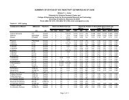
96 Paper No. 03-4207 Transportation Research Record 1842800070006000Riverside Freeway - WeekdayYorba Linda Freeway - WeekdayLa Puente Freeway - Weekday5000400030002000100006 AM7 AM8 AM9 AM10 AM11 AM12 PM1 PM2 PM3 PM4 PM5 PMVolume6 PM7 PM8 PMHour of Day(a)800070006000Riverside Freeway - WeekendYorba Linda Freeway - WeekendLa Puente Freeway - WeekendVolume5000400030002000100006 AM7 AM8 AM9 AM10 AM11 AM12 PM1 PM2 PM3 PM4 PM5 PM6 PM7 PM8 PMHour of Day(b)FIGURE 4 Diurnal freeway average vehicle volume (no. of vehicles per hour) for (a) weekday and (b) weekendin Riverside, Yorba Linda, and La Puente, California.mine vehicle fleet homogeneity in more detail; however, model yearprovided a simple method of identifying differences correlated withemissions.Statistical significance of the differences observed at the threelocations was tested using the two-sample Kolmogorov–Smirnovtest. This nonparametric test identifies differences in distributionbetween two populations (11). In this test, the maximum differencein the cumulative distributions of the two populations is comparedwith a test statistic on the basis of the sample size. For example, ifthe largest difference between two distributions of vehicles occurredwith the 1991 model year and one population had a cumulative distributionof 0.58 (58% 1991 and older) and the second population acumulative distribution of 0.51 (51% 1991 and older), the differencewould be 0.07 (7%). For large samples, this test is effective in detectingdifferences in distribution. The model year cumulative distributionfor the vehicle registration data indicates that the vehicle fleetsregistered in Riverside and Orange Counties are slightly older thanthose in Los Angeles County (Figure 5a). Very small differencesin cumulative percentage were also observed between the vehicleregistration–based fleets in Orange and Riverside Counties.The model year distribution for the on-road mobile vehicle fleetsindicates that the Los Angeles County vehicle fleet was significantlyolder than that in Riverside County or Orange County (Figure 5b).Very small differences in the cumulative distributions were observedbetween Riverside and Orange Counties. For the on-road destinationdata, the differences in the three cumulative distributions were small(Figure 5c). The maximum observed differences in the distributions aswell as the Kolmogorov–Smirnov test statistics are listed in Table 1.Vehicle model year populations were significantly different at the0.01 significance level if the observed maximum difference wasgreater than the Kolmogorov–Smirnov test value.Riverside and Orange Counties were not significantly different(P = 0.01) for either of the on-road vehicle fleet data sets, as noted onthe table. However, they were significantly different for the vehicleregistration data. Los Angeles County was significantly differentfrom Riverside and Orange Counties (P = 0.01) for all three data sets.Vehicle Emissions ImplicationsCMEM and EMFAC were used to help quantify the effects of vehiclefleets and driving behavior on emissions. As a base-case scenario,CMEM was modeled for the unified cycle for Riverside,Yorba Linda, and La Puente, with the vehicle fleets determinedfrom the vehicle registration database for each area. For the refinedscenario, a composite vehicle trace was created for each city formorning, afternoon, and evening time periods. The traces weremodeled in CMEM with the appropriate vehicle fleet as determined

Malcolm et al. Paper No. 03-4207 97Cumulative Percentage100806040200Vehicle Registration - RIVVehicle Registration - ORAVehicle Registration - LA19701971197219731974197519761977197819791980198119821983198419851986Model Year(a)198719881989199019911992199319941995199619971998Cumulative Percentage100806040200On-Road Mobile - RIVOn-Road Mobile - ORAOn-Road Mobile - LA19701971197219731974197519761977197819791980198119821983198419851986Model Year(b)198719881989199019911992199319941995199619971998Cumulative Percentage100806040200On-Road Destination - RIVOn-Road Destination - ORAOn-Road Destination - LA1970197119721973197419751976197719781979198019811982198319841985Model Year(c)1986198719881989199019911992199319941995199619971998FIGURE 5 Cumulative distribution by model year for Los Angeles (LA), Orange (ORA), and Riverside (RIV)Counties for (a ) vehicle registration address data, (b) on-road data, and (c) on-road destination vehicle fleets.TABLE 1 Kolmogorov–Smirnov (KS) Test Summary of Fleet Differences forLos Angeles (LA), Orange (ORA), and Riverside (RIV) CountiesDataset Comparison KS Test Value Maximum Difference*Vehicle Registration KS LA-ORA 0.011 0.034Vehicle Registration KS LA-RIV 0.017 0.064Vehicle Registration KS ORA-RIV 0.019 0.061On-Road Mobile KS LA-ORA 0.067 0.160On-Road Mobile KS LA-RIV 0.063 0.134On-Road Mobile KS ORA-RIV 0.062 0.060 aOn-Road Destination KS LA-ORA 0.023 0.062On-Road Destination KS LA-RIV 0.033 0.078On-Road Destination KS ORA-RIV 0.037 0.018 a* Maximum percent difference between cumulative distributions.a Populations are not significantly different

98 Paper No. 03-4207 Transportation Research Record 1842TABLE 2 CMEM CO, HC, and NO x Emissions for aRegistration Fleet and an On-Road FleetCMEM/DMV (g/mi) Riverside Yorba Linda La PuenteCO 17.31 18.77 16.96HC 1.57 1.83 1.59NOx 1.22 1.36 1.21CMEM/On-Road (g/mi) Riverside Yorba Linda La PuenteCO 10.93 7.66 12.92HC 0.54 0.42 0.64NOx 0.81 0.61 0.75by the on-road SELEV study and normalized based on volume percentagesfor each time period. The time periods were modeled separatelyto account for diurnal differences in driving behavior. Theresulting emissions are listed in Table 2. Using the vehicle tracesand vehicle fleets captured on road, emissions were 25% to 77%lower than when a subsample of the registration database was usedwith a standard cycle.For a secondary comparison, EMFAC 2.08 was modeled forRiverside, Orange, and Los Angeles Counties using the default settingsfor calendar year 2001. The vehicle fleet distribution foundfrom the on-road, in-transit fleet was applied to the total populationof passenger automobiles, light-duty trucks, and medium-duty trucksfor each county. The adjusted vehicle fleets by model year wereentered into EMFAC, and the model was run. The resulting emissionsare listed in Table 3. Using the on-road vehicle fleet data,emissions were 22% to 45% lower than those using the registrationdatabase for the entire county (i.e., the EMFAC default).SUMMARY AND CONCLUSIONSDifferences in the speed–acceleration distribution were identifiedamong Los Angeles, Riverside, and Orange Counties. The vehicleactivity distribution for Riverside County was the fastest on averageand had the lowest proportion of high-congestion speeds. The speedprofiles for the sites in Los Angeles and Orange Counties were similar,but Los Angeles County had a much narrower range of accelerationsand decelerations. The main factor influencing the changesin the speed–acceleration distributions was the congestion leveltypical of each area studied.Differences in the vehicle fleet were identified among the threeareas for the vehicle registration address data set. For the two onroaddata sets, Los Angeles County had a significantly older vehiclepopulation than Riverside County or Orange County. However,Riverside and Orange Counties did not have significantly differentmodel year distributions for either on-road data set.TABLE 3 EFMAC CO, HC, and NO x Emissions for theDefault Fleet and an On-Road FleetEMFAC (g/mi) Riverside Orange Los AngelesCO 8.69 7.15 9.61HC 0.44 0.36 0.52NOx 1.03 0.83 1.05EMFAC/On-Road (g/mi) Riverside Orange Los AngelesCO 5.15 4.32 6.31HC 0.24 0.21 0.33NOx 0.71 0.56 0.82These results lead to several important conclusions:• Differences in vehicle fleet mix, driving behavior, and particularlythe interaction of fleet and driving within the SoCAB resultedin large differences in emissions estimates for the three sites studied.These findings imply that emissions estimates based on regional averagevehicle fleets and average driving speeds may not be accurate,because the average fleet and average driving do not necessarilymatch.• Characterization of vehicle activity with summary statisticssuch as average speed may not adequately characterize the activityfor use in the new-generation models of mobile-source emissions.• Differences in the vehicle activity characteristics were spatiallyas well as temporally heterogeneous.• Changes in the speed–acceleration characteristics of eachlocation were correlated to the level of congestion in that area.• Differences in the age of the vehicle fleet were identified amonggeographic locations studied.• Differences in the age of the vehicle fleet were identified betweentwo of the geographic regions in the vehicle registration addressdata, but no differences in the fleets were found in the on-road data.REFERENCES1. Lents, J., N. Nikkila, N. Davis, and T. Younglove. Mobile Source EmissionsInventory for Zion and Arches National Parks. Proc., 11th CRCOn-Road Vehicle Emissions Workshop. Coordinating Research Council,Alpharetta, Ga., 2001.2. California Air Resources Board EMFAC Model. CARB, Sacramento,Calif. www.arb.ca.gov/msei/msei.htm. Accessed July 31, 2002.3. Guensler, R., S. Washington, and W. Bachman. Overview of the MEA-SURE Modeling Framework. In Transportation Planning and Air QualityIII: Emerging Strategies and Working Solution. American Society ofCivil Engineers, Reston, Va., 1998, pp. 51–70.4. Barth, M., F. An, T. Younglove, C. Levine, G. Scora, M. Ross, andT. Wenzel. The Development of a Comprehensive Modal EmissionsModel. Final Report. National Cooperative Highway Research Program,Nov. 1999.5. Granell, J. L., R. Guensler, and W. H. Bachman. Using Locality-Specific Fleet Distributions in Emissions Inventories: Current Practice,Problems, and Alternatives. Presented at 81st Annual Meeting of theTransportation Research Board, Washington, D.C., 2002.6. Malcolm, C., T. Younglove, J. Tietjen, M. Barth, N. Davis, and J. Lents.Understanding Real-World Vehicle Activity Patterns and Vehicle FleetDistributions in the SoCAB. Proc., 12th CRC On-Road Vehicle EmissionsWorkshop. Coordinating Research Council, Alpharetta, Ga., 2002.7. Younglove, T., C. Malcolm, G. Scora, and M. Barth. Observed On-RoadVehicle Fleet Differences and Their Effect on Emissions. Proc., 12th CRCOn-Road Vehicle Emissions Workshop. Coordinating Research Council,Alpharetta, Ga., 2002.8. Autoscope. Autoscope Supervisor Tool Kit. Econolite, 1999. www.autoscope.com. Accessed July 31, 2002.9. Barth, M., C. Malcolm, T. Younglove, N. Davis, and J. Lents. DevelopingLink Emission Factors in the Southern California Air Basin.Proc., 12th CRC On-Road Vehicle Emissions Workshop. CoordinatingResearch Council, Alpharetta, Ga., 2002.10. Younglove, T., A. Ayala, T. Durbin, S. Kidd, C. Malcolm, M. Smith,and J. Gaskins. Overview and Results of a Statewide Survey of VehicleRegistration Status in California. Proc., 11th CRC On-Road VehicleEmissions Workshop. Coordinating Research Council, Alpharetta,Ga., 2001.11. Siegel, S. Nonparametric Statistics for the Behavioral Sciences.McGraw-Hill Book Company, New York, 1956, pp. 127–136.Publication of this paper sponsored by Committee on Transportation and AirQuality.