Hermitian varieties over finite fields - Matematica

I hereby declare that this thesis has not been submitted, either inthe same or different form, to this or any other University for adegree.Signature:

CONTENTS3.2 Hermitian matrices and polynomials . . . . . . . . . . . . . . . . . . . . . . . 733.2.1 Some general considerations on Hermitian pencils . . . . . . . . . . . 78Further linear algebra observations . . . . . . . . . . . . . . . . . . . . 793.2.2 Case I: 3 or 4 distinct roots . . . . . . . . . . . . . . . . . . . . . . . . 813.2.3 Case II: 2 distinct roots . . . . . . . . . . . . . . . . . . . . . . . . . . 823.2.4 Case III: 1 root . . . . . . . . . . . . . . . . . . . . . . . . . . . . . . 843.2.5 Case IV: some notes when the factorisation contains irreducibles . . . . 873.3 Construction of the incidence configurations . . . . . . . . . . . . . . . . . . . 903.3.1 Pencils with degenerate surfaces of rank 3 only . . . . . . . . . . . . . 903.3.2 Pencils with degenerate surfaces of rank 2 only . . . . . . . . . . . . . 923.3.3 Pencils whose degenerate surfaces have rank 2 and 3 . . . . . . . . . . 934 General results 974.1 The cardinality formula . . . . . . . . . . . . . . . . . . . . . . . . . . . . . . 974.1.1 Introduction . . . . . . . . . . . . . . . . . . . . . . . . . . . . . . . . 974.1.2 Preliminaries . . . . . . . . . . . . . . . . . . . . . . . . . . . . . . . 974.1.3 The determinantal variety H . . . . . . . . . . . . . . . . . . . . . . 1014.1.4 Action of PGL(n + 1, q) on H . . . . . . . . . . . . . . . . . . . . . 1064.1.5 The order formula . . . . . . . . . . . . . . . . . . . . . . . . . . . . 1084.1.6 Some further remarks on H . . . . . . . . . . . . . . . . . . . . . . . 1104.2 Explicit computations and algorithms . . . . . . . . . . . . . . . . . . . . . . 1124.2.1 The computer code: general remarks . . . . . . . . . . . . . . . . . . . 1124.2.2 Initialization:main and param . . . . . . . . . . . . . . . . . . . . . . . . . . . . 1134.2.3 Auxiliary functions:Projective and Helpers . . . . . . . . . . . . . . . . . . . . . . 1144.2.4 Preliminary computations:Prelim.gap . . . . . . . . . . . . . . . . . . . . . . . . . . . . . . 1254.2.5 Unitary group construction:Unitary.gap . . . . . . . . . . . . . . . . . . . . . . . . . . . . . 1294.2.6 Orbit computation:Orbits.gap . . . . . . . . . . . . . . . . . . . . . . . . . . . . . . 1314.2.7 Intersection and results output:Post-orb.gap . . . . . . . . . . . . . . . . . . . . . . . . . . . . . 1324.2.8 Generators of the projective unitary group . . . . . . . . . . . . . . . . 138Quasi-symmetries . . . . . . . . . . . . . . . . . . . . . . . . . . . . 138Ishibashi’s theorem . . . . . . . . . . . . . . . . . . . . . . . . . . . . 140Construction of the matrices . . . . . . . . . . . . . . . . . . . . . . . 142vii

CONTENTS4.2.9 Concluding remarks . . . . . . . . . . . . . . . . . . . . . . . . . . . 143Bibliography 147viii

List of Figures1.1 Veblen-Young configuration . . . . . . . . . . . . . . . . . . . . . . . . . . . 121.2 Desargues configuration . . . . . . . . . . . . . . . . . . . . . . . . . . . . . 131.3 Pappus configuration . . . . . . . . . . . . . . . . . . . . . . . . . . . . . . . 142.1 Possible configurations for the 2-dimensional case . . . . . . . . . . . . . . . . 41ix

List of Tables2.1 Possible intersection numbers for non-degenerate Hermitian Curves. . . . . . . 382.2 Minimal polynomials corresponding to given rank sequences in the 2-dimensionalcase. . . . . . . . . . . . . . . . . . . . . . . . . . . . . . . . . . . . . . . . . 402.3 Canonical forms for 3 by 3 Hermitian matrices. . . . . . . . . . . . . . . . . . 402.4 Equations for the non-degenerate Hermitian curve . . . . . . . . . . . . . . . . 44≠3.1 Possible intersection numbers for Hermitian surfaces: non-degenerate pencil. . 623.2 Possible intersection numbers for Hermitian surfaces: degenerate pencil; r 3 ≠0, r 4 = 0. . . . . . . . . . . . . . . . . . . . . . . . . . . . . . . . . . . . . . 623.3 Possible intersection numbers for Hermitian surfaces: degenerate pencil; r 20, r 3 = r 4 = 0. . . . . . . . . . . . . . . . . . . . . . . . . . . . . . . . . . . 623.4 Possible intersections E between a cone and a non degenerate Hermitian surface;vertex not in the intersection. . . . . . . . . . . . . . . . . . . . . . . . . 643.5 Indices for the intersection of a cone and a Hermitian surface. . . . . . . . . . . 653.6 Possible incidence classes for two non-degenerate Hermitian surfaces: Γ containsdegenerate surfaces of rank 3 only. . . . . . . . . . . . . . . . . . . . . . 683.7 Possible incidence classes for two non-degenerate Hermitian surfaces: Γ containsdegenerate surfaces of rank 2 only. . . . . . . . . . . . . . . . . . . . . . 703.8 Indices for the intersection of Hermitian surfaces of rank 2 and of rank 3. . . . 713.9 Possible incidence classes for two non-degenerate Hermitian surfaces: Γ containsdegenerate surfaces of ranks 2 and 3. . . . . . . . . . . . . . . . . . . . . 743.10 Canonical forms for the 3-dimensional case: M H (x) splits over GF( √ q); 2 or3 distinct roots. . . . . . . . . . . . . . . . . . . . . . . . . . . . . . . . . . . 753.11 Canonical forms for the 3-dimensional case: M H (x) splits over GF( √ q); 1 or4 roots. . . . . . . . . . . . . . . . . . . . . . . . . . . . . . . . . . . . . . . 763.12 Canonical forms for the 3-dimensional case: M H (x) does not split over GF( √ q);degree 4. . . . . . . . . . . . . . . . . . . . . . . . . . . . . . . . . . . . . . . 774.1 Intersection numbers for non-degenerate Hermitian varieties in dimension 4. . . 1104.2 Dimension of the varieties O ≥t for small n . . . . . . . . . . . . . . . . . . . . 111x

IntroductionA projective space PG(n, q) admits at most three types of polarity: orthogonal, symplectic andunitary. The absolute points of an orthogonal polarity constitute a non-degenerate quadric inPG(n, q); for a symplectic polarity, all the points of PG(n, 2 t ) are absolute; the locus of allabsolute points of a unitary polarity is a non-degenerate Hermitian variety.Non-degenerate Hermitian varieties are unique in PG(n, q) up to projectivities. However,two distinct Hermitian varieties might intersect in many different configurations. Our aim inthis thesis is to study such configurations in some detail.In Chapter 1 we introduce some background material on finite fields, projective spaces,collineation groups and Hermitian varieties.Chapter 2 deals with the two-dimensional case. Kestenband has proven that two Hermitiancurves may meet in any of seven point-line configurations. In Section 2.1, we present thisclassification. In Section 2.2, we verify that any two configurations belonging to the same classare, in fact, projectively equivalent and we determine the linear collineation group stabilizingeach of them. Such a group is usually quite large and is transitive on almost all the points ofthe intersection. A subset U of PG(2, q) such that any line of the plane meets U in either 1 or√ q + 1 points is called a unital. A Hermitian curve is a classical unital. However, there existnon-classical unitals as well. In Section 2.3 we present a short proof of a characterisation of theHermitian curve as the unital stabilized by a Singer subgroup of order q − √ q + 1.In Chapter 3, we describe the point-line-plane configurations arising in dimension 3 fromintersecting two Hermitian surfaces. Our approach consists first in determining some combinatorialproperties the configurations have to satisfy and then in actually constructing all thepossible cases. Section 3.1 presents the list of all possible intersection classes; after some moretechnical results in Section 3.2, in Section 3.3 we construct linear systems of Hermitian surfacesyielding the wanted configurations for any class. In this chapter we deal with intersectionswhich contain at least √ q + 1 points on a line.Chapter 4 is divided into two independent sections: in Section 4.1 we study the determinantalvariety of all the (n+1)×(n+1) Hermitian matrices as a hypersurface of PG(n 2 +2n, √ q).From the study of such a variety we are able to determine the list of all possible intersectionsizes for any dimension n. In Section 4.2 we present some computer code in order to producepencils of Hermitian varieties in PG(n, q). This code, however, is able to provide useful re-1

sults only for small values of n and q. Some possible improvements, both from the theoreticstandpoint and the computational one, are suggested.2

Chapter 1Preliminary resultsThe aim of this first chapter is to recall some known results that will be used throughout thethesis.1.1 Permutation GroupsOur main reference for the theory of finite permutation groups is [Wie64]. For general resultson group theory, [Rob80] has been used.1.1.1 DefinitionsDefinition 1.1.1. Let X be a non-empty set. A permutation of X is a bijective mapping of Xinto itself. The set of all permutations of X, together with map composition forms a group S X ,the symmetric group on X.Definition 1.1.2. A permutation group G on a set X, or an X-permutation group, is any subgroupof S X . The degree of a permutation group G is the cardinality of the set X it acts upon.Definition 1.1.3. Let G be an X-permutation group and define † as the equivalence relation onX given byx † y ⇐⇒ ∃σ ∈ G : x = σ(y).The equivalence classes of † are the orbits of G on X. The orbit of any x ∈ X will be denotedby the symbol x G .1.1.2 Transitivity and regularityDefinition 1.1.4. A permutation group G is transitive on X if and only if it has only one orbit,namely X itself.3

CHAPTER 1. PRELIMINARY RESULTS1.1. PERMUTATION GROUPSDefinition 1.1.5. For any X-permutation group G and for any Y ⊆ X, the stabilizer of Y in Gis the setSt G (Y ) := {σ ∈ G : ∀y ∈ Y : σ(y) ∈ Y }.A group G is semi-regular if for any x ∈ X, St G (x) = 1; G is regular if it is semi-regular andtransitive.Definition 1.1.6. Let n be a positive integer. A permutation group G is 1-transitive on X if andonly if it is transitive on X. A group G is n-transitive on a set X if and only if for any x ∈ X,St G (x) is (n − 1)-transitive on X \ {x}.Lemma 1.1.7. Assume that G is a n-transitive group on X. Then,(i) for any x ∈ X, St G (x) is (n − 1)-transitive on X \ {x};(ii) given two tuples l x = (x 1 , . . . , x n ), l y = (y 1 , . . . , y n ) of elements of X, there exists apermutation σ ∈ G such that σ(l x ) = l y .Definition 1.1.8. A group G is strictly n-transitive on X if it is n-transitive and, given any twodifferent n-tuples l x , l y of distinct elements of X, there exists exactly one σ ∈ G such thatσ(l x ) = l y .Lemma 1.1.9. Let G be a permutation group on a set X. Then, for any x ∈ X,1.1.3 Similarities|G| = |x G ||St G (x)|.Definition 1.1.10. Let G be an X-permutation group and H be a Y -permutation group. Asimilarity between G and H is a pair (α, β), where(i) α is an isomorphism between G and H;(ii) β is a bijection between X and Y ;(iii) for any σ in G and for any x ∈ X,β(x σ ) = (β(x)) α(σ) .Two permutation groups are similar if there is a similarity between them.The sets X and Y have to be isomorphic in order for G and H to be similar; still, |X| = |Y |and G ≃ H is not sufficient for G and H to be similar.4

CHAPTER 1. PRELIMINARY RESULTS1.2. FINITE FIELDS1.1.4 Actions and representationsDefinition 1.1.11. Let G be a group and let X be a non-empty set. A right action of G on X isa function ρ : X × G → X such thatρ(x, g 1 g 2 ) = ρ(ρ(x, g 1 ), g 2 ).In an analogous way, a left action of G on X is defined as a function λ : G × X → X such thatλ(g 1 g 2 , x) = λ(g 1 , λ(g 2 , x)).Definition 1.1.12. Let G be any group and let X be a set. Any group homomorphism γ :G → S X is a permutation representation of G on X and it induces a right action on X via themapping (x, g) → γ(g)x.The cardinality of X is the degree of the representation γ. If ker γ = {1}, then the representationis faithful; a representation is transitive if its image in S X is transitive; γ is regular ifits image in S X acts regularly on X.1.2 Finite fieldsThe reference text for most of the definitions and results presented in this section is [LN97].1.2.1 Definitions and modelsDefinition 1.2.1. A ring (R, +, ·) is an integral domain if, for all x, y ∈ R, xy = 0 impliesx = 0 or y = 0; if (R \ {0}, ·) is a group, then the ring R is a division ring. A division ring Rin which the group R ⋆ = (R \ {0}, ·) is Abelian is a field; a division ring in which the group R ⋆is non-commutative is a skew-field.Theorem 1.2.2 (Wedderburn, 1905). Every finite division ring is a field.Definition 1.2.3. The characteristic of a ring (R, +, ·) is the smallest positive integer char(R) =n such that for all r ∈ R:nr := r}+ .{{. . + r}= 0.n timesIf no such an n exists, R is said to have characteristic 0.Definition 1.2.4. A subfield K of a field (F, +, ·) is a subset of F which is closed under thefield operations. The field (F, +, ·) is called an extension (field) of (K, + | K , · | K ). The symbolK ≤ F is used to denote that F is an extension field of K or, equivalently, that K is a subfieldof F .5

CHAPTER 1. PRELIMINARY RESULTS1.2. FINITE FIELDSAny field contains itself, the empty set and the set consisting of its zero only as subfields.Those subfields are called trivial.Definition 1.2.5. A field is prime if it does not contain any proper subfield.Lemma 1.2.6. Any subfield has the same characteristic as its parent field.Definition 1.2.7. Let K be a subfield of F and assume f ∈ F . The extension of K by f is thesmallest subfield K(f) of F such that,K ∪ {f} ⊆ K(f) ⊆ F.Definition 1.2.8. Given a field K, its algebraic closure K is the smallest field containing Ksuch that any polynomialn∑k i x i ∈ K[x]splits to linear factors in K[x].i=0Lemma 1.2.9. Let Z be the ring of integers, p a prime number and let pZ be the ideal generatedby p in Z; then, Z/(pZ) is a finite field containing p elements.Proof. Let F p := {0, . . . , p − 1} ⊂ Z, and let φ be the projection mapping{Fp → Z/(pZ)φ :x → x + (pZ).Define, for any b, c ∈ F ,b + c := φ −1 (φ(b + c));b · c := φ −1 (φ(bc)).The structure (F p , +, ·) is closed under its operations and every non-zero element admits aninverse. It follows that F is a field.Definition 1.2.10. The field (F p , +, ·) constructed in the previous lemma is called the Galoisfield with p elements. It will be denoted by the symbolGF(p) := (F p , +, ·).Definition 1.2.11. Let (F, +, ·) and (G, ⊕, ⊙) be two fields. A morphism between F and G isa mapping φ : F → G preserving the algebraic structure; that is, for all p, q ∈ F :(i) φ(p −1 ) = φ(p) −1 ,(ii) φ(−p) = ⊖φ(p),6

CHAPTER 1. PRELIMINARY RESULTS1.2. FINITE FIELDS(iii) φ(pq) = φ(p) ⊙ φ(q),(iv) φ(p + q) = φ(p) ⊕ φ(q).A necessary condition for a morphism to exist between two fields F and G is that char(F ) =char(G).Monomorphisms, epimorphisms, isomorphisms and automorphisms are defined the usualway.Theorem 1.2.12. Any field K contains a prime subfield F which is either isomorphic to thefield of the rational numbers Q or to GF(p) for some prime p, according as the characteristicof K is 0 or p.Theorem 1.2.13. Let F be a finite field. Then, the cardinality of F is p n , where p = char(F ) isa prime number and n is an integer. The integer n is called the degree of F over its prime field.As a matter of fact, the converse is true as well.Theorem 1.2.14. For every prime p and for every integer n there exists a finite field F of orderp n . All fields of given order q = p n are isomorphic to the splitting field of the polynomial(x q − x) over GF(p). This field F will be written asGF(q) := GF(p)[x]/(x q − x).Definition 1.2.15. Given any finite field (F, +, ·), its multiplicative group F ⋆ is cyclic. A generatorof F ⋆ is a primitive element of F .1.2.2 Automorphisms and extensionsLemma 1.2.16. Let F be a finite extension field of GF(q). Then, there exists an integer m > 0such that F = GF(q m ). This integer is the degree of F over GF(q) and is written as[F : GF(q)] := m.Definition 1.2.17. Let GF(q m ) be an extension field of GF(q), and let α ∈ GF(q m ). Theelements α, α q , . . . , α qm−1 are called the conjugates of α with respect to GF(q).Definition 1.2.18. An automorphism of GF(q m ) over GF(q) is a field automorphism of GF(q m )which fixes all the elements of GF(q). The group of all these automorphisms is the Galois groupof GF(q m ) over GF(q) and it is denoted by the symbolGal(GF(q m ) : GF(q)).Lemma 1.2.19. For any t ∈ GF(q),t q − t = 0.7

CHAPTER 1. PRELIMINARY RESULTS1.2. FINITE FIELDSTheorem 1.2.20. The elements of Gal(GF(q m ) : GF(q)) can be described as the automorphismsσ 0 , σ 1 , . . . , σ m−1 given by{ GF(q m ) → GF(q m )σ j :x → σ j (x) = x qj .The automorphism σ 1 which generates the Galois group is called the Frobenius automorphism.Lemma 1.2.21. Let K be a field and let σ be one of its automorphisms. Then, the set Fix K σ isa subfield of K. This subfield is called the fixed field of σ in K.Corollary 1.2.22. The following equality holds:| Gal(GF(q m )) : GF(q))| = m = [GF(q m ) : GF(q)].Definition 1.2.23. An automorphism σ is involutory if(i) σ is not the identity;(ii) σ 2 is the identity.For any prime-power q, the field F = GF(q 2 ) admits one and only one non-identity automorphismover GF(q), namely the mapping sending x → x q . Since | Gal(F : GF(q))| = 2,this is an involutory automorphism of F .Lemma 1.2.24. Let K be a field and let σ be an involution of K. Then, there exist a subfieldK ′ ≤ K and an element i ∈ K such that,(i) [K : K ′ ] = 2;(ii) K ′ is fixed by σ;(iii) K = K ′ (i).1.2.3 Trace and normLet F and K be finite fields with K ≤ F . From Theorem 1.2.14, it is possible to assumewithout loss of generality that F = GF(q m ), K = GF(q) with q, m integers and q a primepower.Definition 1.2.25. The trace over K of an element x ∈ F is given by∑T F/K (x) := σ(x) = x + x q + . . . + x qm−1 .σ∈Gal(F :K)The trace of x over the prime subfield of F is the absolute trace of x and is simply denoted asT F (x).8

CHAPTER 1. PRELIMINARY RESULTS1.2. FINITE FIELDSTheorem 1.2.26. For any x, y ∈ F and f, g ∈ K, the trace T F/K satisfies the followingproperties.(i) T F/K (x + y) = T F/K (x) + T F/K (y);(ii) T F/K (fx) = fT F/K (x);(iii) T F/K is a linear transformation from F onto K, where both F and K are viewed as vectorspaces over K;(iv) T F/K (f) = mf;(v) T F/K (x q ) = T F/K (x).Theorem 1.2.27. Let K be a finite field, and let F a finite extension of K. The linear transformationsfrom F into K, both seen as vector spaces over K, are exactly the mappings L t fort ∈ F given byAlso, L t ≠ L t ′ when t ≠ t ′ .L t :{ F → Kx → T F/K (tx).Theorem 1.2.28 (Composition of traces). Assume K ≤ F ≤ E to be all finite fields. Then, forany x ∈ E,T E/K (x) = T F/K (T E/F (x)).Definition 1.2.29. The norm over K of an element x ∈ F is given by∏N F/K (x) := σ(x) = x (qm−1)/(q−1) .σ∈Gal(F :K)The norm of x over the prime subfield of F is the absolute norm of x and is simply denoted byN F (x).Theorem 1.2.30. For any x, y ∈ F and f, g ∈ K, the norm N F/K satisfies the followingproperties.(i) N F/K (xy) = N F/K (x)N F/K (y);(ii) N F/K maps F onto K and F ⋆ onto K ⋆ ;(iii) N F/K (f) = f m ;(iv) N F/K (x q ) = N F/K (x).Theorem 1.2.31 (Composition of norms). Assume K ≤ F ≤ E to be all finite fields. Then, forany x ∈ E:N E/K (x) = N F/K (N E/F (x)).9

CHAPTER 1. PRELIMINARY RESULTS1.3. PROJECTIVE SPACES1.3 Projective spacesGood references for the results presented in this section are [Dem68], [KSW73] and [BR98].1.3.1 Incidence structuresDefinition 1.3.1. A triple (P, L, I) is a linear space if(i) P, L are non-empty sets;(ii) I is a symmetric relation on (P × L) ∪ (L × P );(iii) for all distinct x, y ∈ P there exists exactly one element l := xy of L such that (x, l) ∈ Iand (y, l) ∈ I.The elements of P are the points of (P, L, I); those of L are called the lines of the incidencestructure. The relation I is named incidence relation.Definition 1.3.2. In a linear space (P, L, I) two lines l, m intersect if there exist a point x ∈ Psuch that (x, l) ∈ I and (x, m) ∈ I. The notationwill be used.l ∩ m := {x ∈ P : (x, l) ∈ I and (x, m) ∈ I}Definition 1.3.3. Three distinct points x, y, z in a linear space (P, L, I), are called collinear if(x, yz) ∈ I.Definition 1.3.4. A mapping φ from a linear space (P, L, I) to a linear space (P ′ , L ′ , I ′ ) is acollineation (or isomorphism) if(i) φ(p) ∈ P ′ , for all p ∈ P ;(ii) φ(l) ∈ L ′ , for all l ∈ L;(iii) φ is bijective on P ;(iv) the incidence relation is preserved, that is,(p, l) ∈ I ⇐⇒ (φ(p), φ(l)) ∈ I ′ .Definition 1.3.5. Let (P, L, I) be a linear space. A subset U of P is a linear set if, given anytwo distinct points x, y ∈ U,t ∈ xy ⇒ t ∈ U.The fact that U is a linear subset of P is written as U ≤ P .10

CHAPTER 1. PRELIMINARY RESULTS1.3. PROJECTIVE SPACESLemma 1.3.6. Assume (P, L, I) to be a linear space. For any linear subset U of P , let(i) L U := {l ∈ L : ∃ x, y ∈ U such that x ≠ y, (x, l) ∈ I, (y, l) ∈ I};(ii) I U := I | U×LU ∪L U ×U.Then, (U, L U , I U ) is a linear space.Definition 1.3.7. Given two linear spaces (P, L, I) and (P ′ , L ′ , I ′ ), we say that (P ′ , L ′ , I ′ ) is asubspace of (P, L, I) with support P ′ if(i) P ′ ≤ P ;(ii) L ′ = L P ′;(iii) I ′ = I P ′.Definition 1.3.8. Given a linear space (P, L, I) and a set V ⊆ P , the linear set V spanned byV is given byV := ⋂ {T ≤ P : V ⊆ T }.Lemma 1.3.9. For any V ⊆ P , the linear set spanned by V is characterised as follows:V := {x ∈ P : ∃h, k ∈ V such that h ≠ k, (x, hk) ∈ I}.Definition 1.3.10. A projective space (P, L, I) is a linear space in which the following axiomsare satisfied:(i) (Veblen-Young) If a, b, c, d ∈ P are distinct points, thenab ∩ cd ≠ ∅ ⇒ ac ∩ bd ≠ ∅;(ii) any line is incident with at least three points;(iii) there are at least two lines.A finite projective space is a projective space in which the set of points is finite.Definition 1.3.11. A projective plane (P, L, I) is a projective space in which any two linesintersect.Definition 1.3.12. The dimension of a projective space P = (P, L, I) is the numberdim P := inf{|U| : U ⊆ P and U = P } − 1.11

CHAPTER 1. PRELIMINARY RESULTS1.3. PROJECTIVE SPACESabdcFigure 1.1: Veblen-Young configurationDefinition 1.3.13. Six distinct points x i , y i with i ∈ {1, 2, 3} in a linear space (P, L, I) constitutea Desargues configuration if(i) there exists c ∈ P such that (x i , cy i ) ∈ I and (y i , cx i ) ∈ I for all i;(ii) no three of the points c, x 1 , x 2 , x 3 and c, y 1 , y 2 , y 3 are collinear;(iii) the points p ij := x i x j ∩ y i y j are collinear.Definition 1.3.14. A projective space (plane) P is Desarguesian if, for any choice of six pointssatisfying (i) and (ii) of the Desargues configuration, condition (iii) holds.Definition 1.3.15. Six distinct points g i , h i for i ∈ {1, 2, 3} in a linear space (P, L, I) constitutethe Pappus configuration if(i) the g i are all collinear;(ii) the h i are all collinear;(iii) the line G := g 1 g 2 meets the line H := h 1 h 2 in a point c that is distinct from any of the g iand any of the h i ;(iv) given q ij := g i h j ∩ g j h i , then (q 12 , q 13 q 23 ) ∈ I.Definition 1.3.16. A projective space (plane) P is Pappian if, for any choice of six pointssatisfying conditions (i), (ii) and (iii) of Pappus configuration, condition (iv) holds as well.12

CHAPTER 1. PRELIMINARY RESULTS1.3. PROJECTIVE SPACESy1cx1x3x2pp2312y2y3pFigure 1.2: Desargues configuration13Theorem 1.3.17. Any projective space of dimension at least 3 is Desarguesian.Still, there exist non-Desarguesian projective planes.Theorem 1.3.18 (Hessenberg). A finite projective plane P is Pappian only if it is Desarguesian.1.3.2 Algebraic constructionsTheorem 1.3.19. Let K be a division ring and let V be a (left) vector space over K of dimensionn ≥ 3. Then, the triple (P, L, ⊆) where(i) P is the set of all 1-dimensional (left) vector subspaces of V ,(ii) L is the set of all 2-dimensional (left) vector subspaces of V ,(iii) ‘⊆’ is the natural inclusion,is a Desarguesian projective space of dimension n − 1.Definition 1.3.20. The symbol P(V ) is used to denote a projective space constructed from avector space V as in Theorem 1.3.19.Theorem 1.3.21 (Projective derivation of a vector space). Let V be a vector space of dimensionn ≥ 3 over a field K. Define(i) 0 := (0, . . . , 0) ∈ V ;(ii) V ⋆ := V \ {0};13

CHAPTER 1. PRELIMINARY RESULTS1.3. PROJECTIVE SPACESg3Gg1g2cq12q13q23h1h2h3HFigure 1.3: Pappus configuration(iii) V i be the set of i-dimensional subspaces of V ;(iv) P := V ⋆ /K ⋆ := {T \ 0 : T ∈ V 1 };(v) L := { X K ⋆ : X ∈ V 2 }.Then, PV := (P, L, ∈) is a (n − 1)-dimensional Pappian projective space which is isomorphicto P(V ).Definition 1.3.22. Let PV n be the projective derivation of a vector space V of dimension n overa field K. Then, V is the underlying vector space of (P, L, ∈). The projection map{ V⋆→ VP :⋆ /K ⋆x → [x] := K ⋆ xis called the projectivisation of V .Theorem 1.3.23. Let V be a vector space over a division ring K; then P(V ) is Pappian if andonly if K is a field.Definition 1.3.24. The symbol PG(n, K) := PK n+1 ≃ P(K n+1 ) denotes the Pappian projectivespace obtained by projectivisation from a vector space of dimension n + 1 over K.Definition 1.3.25. Let (P, L, I) = PG(n, K) be a Pappian projective space. For any given tsuch that −1 ≤ t ≤ n, the symbol PG t (n, K) denotes all projective subspaces of PG(n, K)with dimension t. In particular PG −1 (n, K) = ∅, PG 0 (n, K) = P and PG n (n, K) = {P }.14

CHAPTER 1. PRELIMINARY RESULTS1.3. PROJECTIVE SPACESTheorem 1.3.26 (First representation theorem). Given any Desarguesian projective space P ofdimension n, there exist a division ring K and a vector space V of dimension n + 1 over Ksuch that P is isomorphic to P(V ).Corollary 1.3.27. Let P be a Pappian projective space of dimension n. Then, there exists afield K such that P ≃ PG(n, K).Proof. By Theorem 1.3.18, P is Desarguesian; Theorem 1.3.26 guarantees that P = P(V ),with V a vector space of dimension n over a division ring K; by Theorem 1.3.23, K is a field.Hence, P ≃ PG(n, K).Corollary 1.3.28. Let P be a finite projective space of dimension at least 3. Then, P is Pappian.Proof. From Theorem 1.3.17, P is Desarguesian; hence, P = P(V ) for some vector space Vover a finite division ring K; by Theorem 1.2.2, K is a field. It follows that P is isomorphic toPG(n, q) := PG(n, K). Hence, P is Pappian.Theorem 1.3.29 (Tecklenburg). A Desarguesian finite plane is Pappian.This result can be proved as in Corollary 1.3.28 or in a more direct geometric way, as donein [Tec87]. Due to Theorem 1.3.23, this is equivalent to Wedderburn’s result.1.3.3 MorphismsDefinition 1.3.30. Let V be a vector space over a field K and let σ be an automorphism of K.A semi-linear automorphism of V with companion automorphism σ is a bijection θ from V intoV such that, for all x, y ∈ V and g ∈ K:(i) θ(x + y) = θ(x) + θ(y);(ii) θ(gx) = g σ θ(x).Theorem 1.3.31 (Second representation theorem). For any collineation φ of a Desarguesianprojective space (P, L, I) = P(V ), there exists a semi-linear automorphism θ of V that inducesφ, in the sense that for all x ∈ P ,φ(x) := {θ(t) : t ∈ x}.Definition 1.3.32. Let P = P(V ) be a Desarguesian projective space. A projectivity of P is acollineation of P induced by a linear map of the underlying vector space V .Definition 1.3.33. Let φ be a collineation of the projective space PG(n, K). A point p ∈PG(n, K) is a centre of the collineation φ if(i) φ(p) = p;15

CHAPTER 1. PRELIMINARY RESULTS1.3. PROJECTIVE SPACES(ii) any line L through p is fixed by φ.A hyperplane H of PG(n, K) is an axis of the collineation φ if φ |H is the identity.Theorem 1.3.34. A non-trivial collineation φ of PG(n, K) has at most one centre and one axis;furthermore, φ has a centre if and only if φ has an axis.Definition 1.3.35. A collineation φ is central (or axial) if it has a centre. A central collineationφ whose centre is incident with its axis is called an elation; if the centre of φ is not incident withits axis, then φ is called a homology.Definition 1.3.36. The set of all collineations of the Pappian projective space PG(n, K) isdenoted by the symbolPΓL(n + 1, K);the set of all projectivities of PG(n, K) is written asPGL(n + 1, K).Theorem 1.3.37. For all integers n ≥ 1 and for all fields K, the set PΓL(n + 1, K) togetherwith mapping composition constitutes a group. The set of all projectivities of PG(n, K) is asubgroup of PΓL(n, K).Theorem 1.3.38. Let K be a field, n ≥ 1 and GL(n + 1, K) be the group of all non-singularmatrices of dimension (n + 1) × (n + 1) over K. Then,PGL(n + 1, K) ≃ GL(n + 1, K)/K ⋆ .Definition 1.3.39. The stabilizer of a line of PG(n, K) in PGL(n + 1, K) is the affine lineargroup AGL(n, K).1.3.4 Singer cyclic groupsSinger cyclic groups have been introduced in [Sin38].Definition 1.3.40. A Singer cyclic group of a projective space Π is a collineation group that iscyclic and transitive on the points of Π. A generator of a Singer cyclic group is a Singer cycle.Definition 1.3.41. A projective space Π is cyclic if it admits a Singer cyclic group.Lemma 1.3.42. Any Desarguesian projective space PG(n, q) is cyclic.Lemma 1.3.43. Any Singer cyclic group is transitive on the set of the lines of PG(2, q).Lemma 1.3.44. Any Singer cycle of PG(n, q) is conjugate to a diagonal linear transformationin PGL(n + 1, q n+1 ).16

CHAPTER 1. PRELIMINARY RESULTS1.4. POLYNOMIALS AND MATRICES1.4 Polynomials and matricesThe results in this section are taken from [Lan80] and [HH70].1.4.1 DefinitionsDefinition 1.4.1. Let K be a field. By the symbol Mat(n, K) we denote the ring of all n ×n matrices with entries in K. For any prime power q, the ring Mat(n, GF(q)) is written asMat(n, q).For any given matrix M ∈ Mat(n, K), we write its transposed matrix, obtained interchangingrows and columns of M, as M ⋆ .Definition 1.4.2. Two matrices A, B ∈ Mat(n, K) are equivalent if there exist a matrix C ∈Mat(n, K), such that(i) det C ≠ 0;(ii) A = CBC ⋆ .Definition 1.4.3. Given any matrix M ∈ Mat(n, K), its characteristic polynomial C M (x) iswhere I n is the identity matrix in Mat(n, K).C M (x) := det(M − xI n ),Definition 1.4.4. For any matrix M ∈ Mat(n, K) and any polynomial p(x) = ∑ p i x i ∈ K[x],the valuation of p(x) at M isp(M) := ∑ p i M i .Lemma 1.4.5. Let M ∈ Mat(n, K); the setis an ideal of the ring K[x].J(M) := {p ∈ K[x] : p(M) = 0}Since K[x] is a principal ideal domain, there exist a generator element for J(M) that isunique up to multiplication by elements of K ⋆ .Definition 1.4.6. The minimal polynomial of M ∈ Mat(n, K) is the monic generator M M (x)of the ideal J(M) of K[x].Lemma 1.4.7. For any M ∈ Mat(n, K),(i) deg C M (x) = n;17

CHAPTER 1. PRELIMINARY RESULTS1.5. VARIETIES OVER FINITE FIELDS(ii) C M (x) ∈ J(M);(iii) M M (x) divides C M (x).Definition 1.4.8. The null space of a matrix M ∈ Mat(n, K) is the set Null M of all vectorsx ∈ K n such thatMx ⋆ = 0.Equivalently, the null space of M is the kernel of the homomorphism induced by M. The nullspace of a polynomial p(x) with respect to a matrix M is the setNull M p(x) := {y ∈ K n : p(M)y ⋆ = 0}.1.5 Varieties over finite fieldsThe few general algebraic geometry results presented in this section are from [Ful69]. Referencesfor the GF(q)-case are [Hir98b] and our notes [Hir98a]; the conventions adopted arethose of [Hir98b].1.5.1 Polynomials as functions over projective spacesFor any field K, we shall denote by R n the ring R n (K) := K[X 1 , . . . , X n ] of polynomials inn indeterminates with coefficients in K. This ring is the free ring generated by the symbolsX 1 , . . . , X n over K.Definition 1.5.1. Let K be a field; a form f of degree r in n + 1 variables is a homogeneouspolynomial f ∈ K[X 0 , . . . , X n ] of degree r.Definition 1.5.2. We denote the set of all forms in n + 1 variables over a field K by R n (K) ⊆K[X 0 , . . . , X n ]; the set of all forms in n + 1 variables of given degree r over K is written asR r n(K).Let f ∈ R n (K) be a form, and let V be an n + 1-dimensional vector space over K; for anyvector v = (v 0 , . . . , v n ) ∈ V ≃ K n+1 , the value of f at v is the scalarf(v) := f(v 0 , . . . , v n ).Remark 1.5.3. Neither R n (K) nor R r n(K) are subrings of R n [X 0 ], since the former is notclosed under the sum and the latter under the product. On the other hand, (R n (K) ⋆ , ·) is amonoid and (R r n(K) ∪ {0}, +) is a group.Lemma 1.5.4. Let P = PG(n, K) = PK n+1 be a projective space and consider a form f ∈R n (K). Then, for all v ∈ K n+1 \ {0}, f(v) = 0 impliesf(z) = 0, for all z ∈ Pv.18

CHAPTER 1. PRELIMINARY RESULTS1.5. VARIETIES OVER FINITE FIELDSProof. Since z ∈ Pv, there exists a λ ∈ K ⋆ such that z = λv. Denote by r be the degree of f;then,f(λv) = λ r f(v) = 0.1.5.2 Algebraic sets and idealsDefinition 1.5.5. Let K be a field and assume F := {f 1 , . . . , f k } ⊆ R n (K). The set of zerosdetermined by F isV(F) := V(f 1 , . . . , f k ) := {Pv ∈ PK n+1 : f 1 (v) = f 2 (v) = . . . = f k (v) = 0}.The ideal of F in R n (K) is denoted byI(F) := I(f 1 , . . . , f k ).Lemma 1.5.6. Let F, F ′ ⊆ R n (K), with I(F) = I(F ′ ). Then,V(F) = V(F ′ ).Remark 1.5.7. Lemma 1.5.6 shows that the set V(F) does not depend on the list of forms Fbut only on the ideal F generates in R n (K).Definition 1.5.8. Let K be a field and assume F = {f 1 , . . . , f r } to be a set of forms in R n (K).The projective variety defined by F is the pairThe set I(F) is the ideal of F(F).F(F) := F(f 1 , . . . , f r ) := (V(F), I(F)).Definition 1.5.9. The intersection of two varieties F(F) and F(G) is the projective varietyF(F) ∩ F(G) := F(F ∪ G).Definition 1.5.10. A sub-variety of a variety F(F) is a projective variety F(G) such thatF(G) ∩ F(F) = F(G).Lemma 1.5.11. Let F(F) and F(G) be two projective varieties. Then,F(F) ∩ F(G) = (V(F) ∩ V(G), I(F ∪ G)).Definition 1.5.12. Let F = {f 1 , . . . , f r } ⊆ R n (K) be a set of forms over a field K. A K-rational point of F(F) is an element Pv ∈ V(F) ∩ PG(n, K).Let K denote the algebraic closure of K. A point of F(F) is any P t ∈ PK n+1 such thatf(t) = 0, for all f ∈ F. The set of all points of F(F) isV(F).For any subfield K ′ of K, a K ′ -rational point P t of F(F) is a point of PG(n, K ′ ) ∩ V(F).19

CHAPTER 1. PRELIMINARY RESULTS1.5. VARIETIES OVER FINITE FIELDSDefinition 1.5.13. An algebraic set Y in PG(n, K) is a set of points of PG(n, K) such thatthere exists F ⊆ R n (K), withY = V(F).The ideal of the set Y is defined asĨ(Y ) := I(F).1.5.3 Number of rational points: zeta functionsDefinition 1.5.14. Let X = V(F) be a projective variety over a finite field GF(q). A point P tof X of degree i is a point that is GF(q i )-rational, but is not GF(q j )-rational for any j < i.A closed point of degree i is a setP t := {P t σ : σ ∈ Gal(GF(q i ) : GF(q))} = {P t, P t q , . . . , P t qi−1 },where P t is a point of X of degree i.Definition 1.5.15. A divisor on a curve X = V(F) is an element of the free group generatedby all its closed points.The group of all divisors of X is written as Div(X).Definition 1.5.16. A divisor D is a K-divisor if all its components are K-rational points.Remark 1.5.17. A divisor D on a curve X = V(F) is a formal sumD =∑n P t P t,where(i) n P t ∈ Z;P t∈V(F)(ii) n P t = 0, for all but a finite number of P t;(iii) if P t is a point of X of degree i, then n P t = n P t ′, for all P t ′ ∈ P t.Definition 1.5.18. Let X = V(F) be a projective curve; its zeta function is the formal series∑ζ X (T ) := T deg(D) .D∈Div K (X)Lemma 1.5.19. For any projective curve X = V(F) defined over GF(q), let(i) N i be the number of points of X that are GF(q i )-rational;(ii) M s be the number of effective GF(q)-divisors on X of degree s;20

CHAPTER 1. PRELIMINARY RESULTS1.5. VARIETIES OVER FINITE FIELDS(iii) B j be the number of closed points of degree j.Then,(i)(ii)∞∑ζ X (T ) = 1 + M s T s ;s=1N i = ∑ jB j ;j|i(iii)∞∏∞∑ζ X (T ) = (1 − T j ) −B j= exp( N i T i /i).j=1i=11.5.4 Dimension and algebraic setsLemma 1.5.20. The family of the algebraic sets of PG(n, K) is closed under finite union andintersection; both ∅ and PG 0 (n, K) are algebraic sets.Definition 1.5.21. The Zariski topology on PG 0 (n, K) is the topology whose open sets are thecomplements of algebraic sets.Remark 1.5.22. Any sub-variety F(G) of a projective variety F(F) is closed in F(F).Definition 1.5.23. A non-empty subset Y of a topological space Ξ is irreducible if it cannot beexpressed as the union Y 1 ∪ Y 2 of two proper subsets, each one of which is closed in Y with theinduced topology.The empty set is not irreducible.Definition 1.5.24. The dimension of a topological space Ξ is the supremum of all the integers isuch that there exists a chainZ 0 ⊂ Z 1 ⊂ . . . ⊂ Z n = Ξof distinct irreducible closed subsets.Definition 1.5.25. The dimension of a variety F(F) is the topological dimension of its point setV(F), when endowed with the Zariski topology.Remark 1.5.26. The null form 0 ∈ R n (K) defines the projective varietyF(0) := (PG 0 (n, K), {0}).Its topological dimension is n, the same as the incidence dimension of PG(n, K). This is theonly variety of dimension n in PG(n, K).21

CHAPTER 1. PRELIMINARY RESULTS1.6. UNITARY GROUPSDefinition 1.5.27. Let F(F) be a variety. ByF r (F)we denote the set of all r-dimensional sub-varieties of F(F).Definition 1.5.28. An hypersurface of PG(n, K) is a projective variety of dimension n − 1 inPG(n, K). A 3-dimensional projective variety is a projective surface; a 2-dimensional projectivevariety is a projective curve.1.5.5 Non-singular varietiesDefinition 1.5.29. Let F = {f 1 , . . . , f k } ⊆ R n (K). The Jacobian matrix associated to F at apoint p ∈ K n+1 is the k × (n + 1) matrix J F (p) given bywhere(i) 0 ≤ j ≤ n;(ii) 1 ≤ i ≤ k;(J F (p)) i(j+1) := ∂F i∂X j∣ ∣∣∣p,(iii) ∂F i /∂X j is the formal derivative of F i with respect to X j .Definition 1.5.30. A variety F(F) is non-singular at a point p ∈ V(F) if the rank of its Jacobianmatrix J F (p) at p is maximal, that isrankJ F(p) = (n − dim F(F)).A variety F(F) is non-singular if it is non-singular at each of its points.Definition 1.5.31. Assume Px to be a non-singular point of a variety F(F). The tangent spaceto F(F) at Px is the subspace of PG(n, K) generated by the points corresponding to the projectionof the rows of the Jacobian matrix J F (x).1.6 Unitary GroupsThe results in this section are taken from [Die71] and from the notes of the 1999 SocratesSummer school [Kin99].22

CHAPTER 1. PRELIMINARY RESULTS1.6. UNITARY GROUPS1.6.1 DefinitionsLet V be a vector space over a field K and assume σ to be either an involution of K or theidentity mapping; denote by K ′ the subfield of K fixed by σ.Definition 1.6.1. A sesquilinear form f defined on V is a mapping V × V → K such that, forany choice of x, x 1 , x 2 , y, y 1 , y 2 in V and λ in K,(i) f(x 1 + x 2 , y) = f(x 1 , y) + f(x 2 , y);(ii) f(x, y 1 + y 2 ) = f(x, y 1 ) + f(x, y 2 );(iii) f(xλ, y) = λ σ f(x, y);(iv) f(x, yλ) = f(x, y)λ.Definition 1.6.2. Let f and g be two sesquilinear forms which are respectively defined over thevector spaces X and Y . Then, f and g are equivalent if there exists an isomorphism T of Xinto Y such that, for any x, y ∈ X,f(x, y) = g(T x, T y).Definition 1.6.3. A sesquilinear form f defined on V is non-degenerate if, for any non-zerovector x ∈ V , there exists a vector y ∈ V such thatThe form f is reflexive if, for any x, y ∈ V ,f(x, y) ≠ 0.f(x, y) = 0 ⇐⇒ f(y, x) = 0.Definition 1.6.4. A sesquilinear form f is Hermitian if, for any x, y ∈ V ,f(x, y) = f(y, x) σ .From now on we assume f to be a sesquilinear form on V which is both non-degenerate andreflexive.Definition 1.6.5. A transformation u of V unitary with respect to the form f is any bijectivelinear transformation of V which preserves f. That is, for any x, y ∈ V ,f(x, y) = f(u(x), u(y)).Lemma 1.6.6. The set of all transformations of V unitary with respect to the form f form asubgroup U f (n, K) of the general linear group GL(n, K).23

CHAPTER 1. PRELIMINARY RESULTS1.6. UNITARY GROUPSDefinition 1.6.7. Let θ be an automorphism of the field K. A unitary semi-similarity of V(corresponding to the form f and the automorphism θ) of multiplier r u is a collineation u :V → V such that, for any x, y ∈ V ,f(u(x), u(y)) = r u f(x, y) θ .Lemma 1.6.8. The set of all unitary semi-similarities of V forms a subgroup ΓU f (n, K) of thegroup ΓL(n, K) of all collineations of V .Definition 1.6.9. A semi-similarity u is linear if the automorphism θ associated with u is theidentity of K.Lemma 1.6.10. The set of all linear semi-similarities is a subgroup GU f (n, K) of the generallinear group GL(n, K); indeed,GU f (n, K) = ΓU(n, K) ∩ GL(n, K).Lemma 1.6.11. Let f, g be two equivalent sesquilinear forms. Then, the unitary groups inducedby f and g are all isomorphic; that is, U f (n, K) ≃ U g (n, K), ΓU f (n, K) ≃ ΓU g (n, K) andGU f (n, K) ≃ GU g (n, K).Definition 1.6.12. Let α be in K ⋆ . The dilation of V with coefficient α is the mapping{ V → Vh α :x → xα.Lemma 1.6.13. The set H(n, K) := {h α : α ∈ K ⋆ } of all dilations of V is a normal subgroupof ΓL(n, K).Definition 1.6.14. The group of all projective collineations of the projective space PV , obtainedby derivation from V , is the quotient groupPΓL(n, K) := ΓL(n, K)/H(n, K).The canonical projection from ΓL(n, K) in PΓL(n, K) is denoted as{ ΓL(n, K) → PΓL(n, K)P :x → xH(n, K).Definition 1.6.15. The projective collineation groupsPΓU f (n, K), PGU f (n, K), PU f (n, K)are defined as the images in PΓL(n, K) via the projection P ofΓU f (n, K), GU f (n, K), U f (n, K).24

CHAPTER 1. PRELIMINARY RESULTS1.6. UNITARY GROUPS1.6.2 Subspaces and formsLemma 1.6.16. A necessary and sufficient condition for the existence of a unitary transformationu, mapping a subspace X ≤ V into Y ≤ V , is that the restriction of the form f to X isequivalent to the restriction of the same form f to Y .Definition 1.6.17. A subspace X of V is orthogonal to Y ≤ V with respect to the form f if andonly if, for all x ∈ X and y ∈ Y ,f(x, y) = 0.The largest subspace of V orthogonal to X is denoted asX ⊥ := {v ∈ V : ∀x ∈ X, f(v, x) = 0}.Definition 1.6.18. A space X is isotropic if X ∩ X ⊥ ≠ {0}; it is totally isotropic if X ⊆ X ⊥ .Definition 1.6.19. An hyperbolic plane X is a non-isotropic plane of V containing at least oneisotropic vector.Lemma 1.6.20.(i) If X and Y are two totally isotropic subspaces of V and dim X = dim Y , then there existsan u ∈ U f (n, K), such that u(X) = Y .(ii) There exists an integer ν such that any totally isotropic subspace of V is contained in atotally isotropic subspace of maximal dimension ν.Definition 1.6.21. A quasi-symmetry (with hyperplane H) is a unitary transformation u fixingpoint-wise a non-isotropic hyperplane H in V .Definition 1.6.22. A hyperbolic transformation is a unitary transformation u ∈ U f (n, K) fixingall vectors of a subspace Y ≤ V of dimension n−2 which is orthogonal to an hyperbolic plane.Remark 1.6.23. The projective image PX of an hyperbolic plane X is a hyperbolic line. A projectivehyperbolic transformation is, hence, a unitary transformation fixing all points belongingto a projective hyperplane (PX) ⊥ .1.6.3 Hermitian groupsDefinition 1.6.24. A Hermitian sesquilinear form g is a trace form if, for all v ∈ V , the elementg(v, v) ∈ K can be written as a trace over K ′ ; that is, for any v ∈ V , there exists a λ v ∈ K suchthatg(v, v) = T K/K ′(λ v ).25

CHAPTER 1. PRELIMINARY RESULTS1.6. UNITARY GROUPSLemma 1.6.25. If the characteristic of K is not 2, then all Hermitian sesquilinear forms overK are trace forms. If K has characteristic 2, then the only trace forms are the alternating ones.Definition 1.6.26. The standard Hermitian product on the vector space V is the Hermitiansesquilinear form 〈·, ·〉, given by{ V × V → K〈·, ·〉 :(u, v) → ∑ u i vi σ .For any Hermitian form g equivalent to the standard Hermitian product, the unitary groupsU g (n, K), GU g (n, K), ΓU g (n, K) and PU g (n, K), PGU g (n, K), PΓU g (n, K), are denotedomitting the reference to g; that is, they are simply written as U(n, K), GU(n, K), ΓU(n, K)and PU(n, K), PGU(n, K), PΓU(n, K).For any prime power q, the notation U(n, q) := U(n, GF(q)) will be adopted as well.1.6.4 Generators of the unitary groupTheorem 1.6.27. Let f be a non-alternating symplectic form. Then, either the unitary group isU f (n, K) = U(2, 4), or U f (n, K) is generated by the quasi-symmetries of V ≃ K n .Theorem 1.6.28. Let ν be the dimension of a maximal totally isotropic subspace X of V . Then,(i) if ν ≥ 1, all the transformations in U f (n, K) are products of hyperbolic transformations;(ii) if ν ≥ 1 and n ≥ 3, all non-isotropic lines are the intersection of two hyperbolic planes,except in the case where U f (n, K) coincides with the orthogonal group O(3, 3).1.6.5 Morphisms and automorphismsDefine Z(n, K) as the centre of GL(n, K).Lemma 1.6.29. For any sesquilinear form f, the following isomorphism relations are satisfied:(i) PGL(n, K) ≃ GL(n, K)/Z(n, K);(ii) PΓU f (n, K) ≃ ΓU f (n, K)/H(n, K);(iii) PGU f (n, K) ≃ GU f (n, K)/Z(n, K).Theorem 1.6.30. Suppose g to be a Hermitian form, let n ≥ 3 and assume charK to be odd.Then, all automorphisms of the unitary group U g (n, K) can be written aswhereφ(u) = χ(u)u g ,26

CHAPTER 1. PRELIMINARY RESULTS1.7. HERMITIAN FORMS AND HERMITIAN VARIETIES(i) g ∈ ΓU g (n, K);(ii) χ is an homomorphism of U g (n, K) into its centre.Theorem 1.6.31 (Walter). Let K be a field of odd characteristic with more than 3 elements andassume n ≥ 5. Then, any automorphism of the projective unitary group PU f (n, K) is obtainedfrom an automorphism of U f (n, K) by way of quotienting.1.7 Hermitian Forms and Hermitian varietiesThe main references for this section are [Seg67], [Seg65] and [Hir98b].1.7.1 Hermitian matricesAssume K to be a field with an involutory automorphism σ and let K ′ be the fixed field of σ inK.Definition 1.7.1. Let H ∈ Mat(n, K). Then, H is(i) Hermitian with respect to the automorphism σ, ifH ⋆ = H σ ;(ii) anti-Hermitian with respect to the automorphism σ, ifH ⋆ = −H σ ;(iii) unitary with respect to the automorphism σ, ifH σ = (H ⋆ ) −1 ;(iv) anti-orthogonal with respect to the automorphism σ, ifH σ = H −1 .Lemma 1.7.2. The conjugate of a Hermitian matrix via a unitary matrix is a Hermitian matrix.Lemma 1.7.3. Let H ∈ Mat(n, K) be a Hermitian matrix; then, det H ∈ K ′ .Proof. Since det H = det H ⋆ ,d := det H = det H ⋆ = det H σ = (det H) σ = d σ .Hence, d ∈ Fix K (σ) = K ′ .27

CHAPTER 1. PRELIMINARY RESULTS1.7. HERMITIAN FORMS AND HERMITIAN VARIETIESDefinition 1.7.4. Let V be a vector space over K, and assume H ∈ Mat(n, K) to be a matrix,Hermitian with respect to the automorphism σ. The σ-Hermitian form over V defined by H isthe formh :{ V × V → K(x, y) → x σ Hy ⋆ .Lemma 1.7.5. Assume q to be a square and let H ∈ Mat(n, q) be a Hermitian matrix. Then,αH is a Hermitian matrix for any α ∈ GF( √ q).Definition 1.7.6. A polynomial f(x) in K[x] is Hermitian if and only if, for any integer n andany Hermitian matrix H ∈ Mat(n, K), f(H) is a Hermitian matrix.Remark 1.7.7. All polynomials with coefficients in the subfield K ′ of K are Hermitian.Lemma 1.7.8. The set of all Hermitian matrices of Mat(n, q) is a vector space of dimension n 2over GF( √ q).Proof. A Hermitian H matrix can be given by providing the entries in its upper triangular part;any entry on the main diagonal, that is of the form H ii , is an element of GF( √ q); entries abovethe main diagonal are elements of GF(q); hence, they have the form a + ɛb with a, b ∈ GF( √ q)and ɛ a fixed element of GF(q) \ GF( √ q).A direct count shows that exactlyn + 2( 1 n)(n − 1) = n22choices of elements of GF( √ q) have to be made in order to determine H.Definition 1.7.9. Two matrices A, B ∈ Mat(n, K) are Hermitian-equivalent if there exists anon-singular matrix C ∈ Mat(n, K) such thatA = C σ BC ⋆ .Theorem 1.7.10 (Equivalence of Hermitian matrices). Let H ∈ Mat(n, K) be a Hermitianmatrix of rank n − t. Then, H is Hermitian-equivalent to a matrix J of the formwhere j i ∈ K ′ for any i.J := diag(j 0 , . . . , j n−t , 0, . . . , 0 ),} {{ }t times1.7.2 Hermitian formsLemma 1.7.11 (Representation theorem for Hermitian forms). Let V be a vector space ofdimension n over the field K and let H be a Hermitian matrix in Mat(n, K). Then, the σ-Hermitian form over V defined by H is a sesquilinear Hermitian form in the sense of Definition28

CHAPTER 1. PRELIMINARY RESULTS1.7. HERMITIAN FORMS AND HERMITIAN VARIETIES1.6.4. Conversely, given a sesquilinear Hermitian form h over a vector space V of dimensionn, there exists a Hermitian matrix H ∈ Mat(n, K) such that h is the σ-Hermitian form over Vdefined by H.Thanks to Lemma 1.7.11, it is possible to identify σ-Hermitian forms and sesquilinear Hermitianforms.Remark 1.7.12. Over an arbitrary field K, there might exist different classes of Hermitianforms, depending on the involutory automorphism σ of K which has been chosen. On the otherhand, if K is a finite field GF(q), then there is an involutory automorphism of K if and only ifq is a square. In this case, the involution is unique and it is associated with the subfield of Kwith index 2, that is GF( √ q).Let q be a prime power p 2n . The unique involutory automorphism σ of GF(q) over GF( √ q)will be denoted by the conjugation sign. Namely, for x ∈ GF(q):x := x σ = x √q .Definition 1.7.13. Let r ≥ 1 be an integer and assume V to be a vector space of dimension nover the field K. A mapping h : V n → K is a homogeneous polynomial mapping of degree r ifthere exists a polynomial f ∈ R r n(K) such that{ Vn→ Kh :(p 1 , p 2 , . . . , p n ) → f(p 1 , p 2 , . . . , p n ).Such a polynomial f is said to represent the mapping h.For a vector space V over an arbitrary field K, a σ-Hermitian form h usually cannot berepresented by a polynomial mapping. For instance, there is no polynomial in R 2n (C) whichrepresents the Hermitian form induced over the vector space C n by the standard Hermitianproduct between complex numbers. However, if K is finite, the following theorem is true.Theorem 1.7.14. Let V be a vector space of dimension n over GF(q), with q a square, and√ q+1let h be a Hermitian form defined over V . Then, there exists a polynomial f ∈ R2nwhichrepresents h.Proof. The only involution of GF(q) is the Frobenius automorphism σ : t → t √q . Theorem1.7.11 guarantees that there exists a Hermitian matrix H such that the form h is represented byH. Then,h :{ V × V → K(x, y) → x √q Hy ⋆ .By computing the expansion of the vector/matrix product, this yieldsn∑ n∑h(x, y) = [y j x √ qi H ji ],whence the result.j=129i=1

CHAPTER 1. PRELIMINARY RESULTS1.7. HERMITIAN FORMS AND HERMITIAN VARIETIES1.7.3 Hermitian hypersurfaces: definitionsThis subsection deals only with Hermitian forms which are representable by polynomials. However,the assumption that the field K is finite is not necessary.Definition 1.7.15. The Hermitian hypersurface defined by the Hermitian form h is the algebraicvarietyH(h) := F(f(x, x)),where f is a polynomial representing h and x = (X 0 , . . . , X n ). The Hermitian hypersurfacedefined by the matrix H is the Hermitian hypersurfaceH(H) := H(h),where h is the Hermitian form induced by the matrix H. The algebraic variety F(0), inducedby the trivial Hermitian form, is not considered to be a Hermitian varietyRemark 1.7.16. A Hermitian form h over GF(q) is not a Hermitian form over GF(q i ) for i > 1.However it makes sense to consider the GF(q i )-rational points of the GF(q)-Hermitian varietyH(h).Theorem 1.7.17. The set of all Hermitian hypersurfaces of PG(n, q) can be endowed with thestructure of a PG(n 2 + 2n, √ q).Proof. The correspondence in Lemma 1.7.11 allows us to identify Hermitian forms with Hermitianmatrices. Let H, H ′ be two non-zero Hermitian matrices defining the same Hermitian hypersurface,and call f, f ′ the Hermitian polynomials associated with them. Since F(f(x, x)) =F(f ′ (x, x)), the ideals generated by f(x, x) and f ′ (x, x) have to be the same, that isI(f(x, x)) = I(f ′ (x, x)).It follows that there exists an α ∈ GF(q) ⋆ such thatf(x, x) = αf ′ (x, x).Then, by construction,H = αH ′and α ∈ GF( √ q) ⋆ . An immediate computation shows the converse, namely that if H = αH ′with α ∈ GF( √ q), then H(H) = H(H ′ ).By Lemma 1.7.8, the Hermitian matrices in Mat(n + 1, q) constitute a vector space V overGF( √ q) with dimension (n + 1) 2 .30

CHAPTER 1. PRELIMINARY RESULTS1.7. HERMITIAN FORMS AND HERMITIAN VARIETIESDistinct Hermitian hypersurfaces of PG(n, q) are in one-to-one correspondence with elementsof the set U of all Hermitian polynomials modulo GF(q) ⋆ ; the set U, in turn, is inone-to-one correspondence with the quotient spaceV ⋆ / GF( √ q) ⋆ ,which is isomorphic to PG(n 2 + 2n, √ q) and this proves the theorem.Definition 1.7.18. The rank of a Hermitian hypersurfaceis the rank of the matrix H.H(H) := F(xHx ⋆ )Lemma 1.7.19. A point x on a Hermitian hypersurface H(H) is singular if and only if x belongsto the null-space of H, that isxH = 0.Lemma 1.7.20. A Hermitian hypersurface is non-singular if and only if the matrix associatedwith it has full rank, that is, it is a non-singular matrix.Lemma 1.7.21. Let H and H ′ be two Hermitian-equivalent matrices. Then, the hypersurfacesH(H) and H(H ′ ) are projectively equivalent.Lemma 1.7.22. For any k ≤ n+1, there exists exactly one Hermitian hypersurface in PG(n, q)of rank k up to projectivities.Proof. Theorem 1.7.10 and Lemma 1.7.21 imply that any non-singular Hermitian hypersurfacein PG(n, q) is projectively equivalent to the one generated by the diagonal matrixM := diag(m 0 , . . . , m k , 0, . . . , 0),where m 0 , . . . , m k are in GF( √ q). Since the norm from GF(q) onto GF( √ q) is surjective,there exist elements t i ∈ GF(q), such thatt i t i = m i .Let T be the matrixT := diag(t 0 , . . . , t k , 0, . . . , 0).Then, M is Hermitian-equivalent via T to the block matrixwhere I k is the k × k identity matrix.diag(I k , 0, . . . , 0} {{ }),n + 1 − k times31

CHAPTER 1. PRELIMINARY RESULTS1.7. HERMITIAN FORMS AND HERMITIAN VARIETIESDefinition 1.7.23. The canonical Hermitian hypersurface of rank k in PG(n, q) is the HermitianhypersurfaceΠ n−k−1 U k,qinduced by the matrix diag(I k+1 , 0, . . . , 0) ∈ Mat(n + 1, q). The canonical non-singular Hermitianhypersurface in PG(n, q) is the non-singular Hermitian hypersurfacewhere I is the identity of Mat(n + 1, q).U n := Π −1 U n,q := H(I),A Hermitian hypersurface which is projectively equivalent to a Π n−1 U 0,q is a hyperplanerepeated √ q + 1 times; a Hermitian hypersurface projectively equivalent to a Π n−k−1 U k,q is aHermitian cone having as vertex a Π n−k−1 ∈ PG n−k−1 (n, q) and base a U k,q .Definition 1.7.24. The canonical Hermitian norm of rank k in PG(n, q) is the formh k,n (x) :=With Definition 1.7.24, we can write(i) U n := F(h n,n (x));(ii) Π n−k−1 U k := F(h k,n (x)).k∑x i x i =i=0k∑i=0x √ q+1i .1.7.4 Hermitian sub-varieties and pointsLemma 1.7.25. The intersection of a Hermitian H variety with a subspace Π r ∈ PG r (n, q) ofdimension r not completely included in H is a Hermitian variety of Π r .Corollary 1.7.26. The intersection of a Hermitian variety with a line is either a line, a Baersubline or a point.Proof. The corollary follows by observing that Hermitian varieties in dimension 1 are eitherBaer sublines or lines (if completely degenerate), while a Hermitian variety in dimension 0 is apoint.The following theorems deal with the cardinality of the set of the points of a (possiblysingular) Hermitian variety H.Theorem 1.7.27. The zeta function of the non-singular Hermitian curve U 2,q isζ U2,q (T ) = (1 + √ qT ) q−√ q(1 − T )(1 − qT ) .32

CHAPTER 1. PRELIMINARY RESULTS1.7. HERMITIAN FORMS AND HERMITIAN VARIETIESTheorem 1.7.28. The number of GF(q)-rational points of the non-singular Hermitian varietyU n,q isµ(n, q) := [q (n+1)/2 + (−1) n ][q n/2 − (−1) n ]/(q − 1).Corollary 1.7.29.(i) µ(1, q) = √ q + 1;(ii) µ(2, q) = q √ q + 1;(iii) µ(3, q) = (q + 1)(q √ q + 1).Theorem 1.7.30. The singular Hermitian variety Π m U k,q contains:(i) q m + q m−1 + . . . + 1 = (q m+1 − 1)/(q − 1) singular points;(ii) q m+1 µ(k, q) non-singular GF(q)-rational points;(iii) η(m, k, q) = (q m+1 − 1)/(q − 1) + q m+1 µ(k, q) total GF(q)-rational points.1.7.5 Hermitian varieties and unitary groupsThe stabilisers of a Hermitian variety U n,q in the collineation groups of PG(n, q) are unitarygroups. In fact, the following lemma holds true.Lemma 1.7.31. The stabiliser in PGL(n + 1, q) of the set of the GF(q)-rational points of U n,qis PGU(n + 1, q). The stabiliser of the same set in PΓL(n + 1, q) is PΓU(n + 1, q).Definition 1.7.32. The group PγU(n + 1, q) is the group of all collineations of PG(n, q) stabilizingthe point set of U n,q which are associated either with the identity of the field GF(q) orwith its involutory automorphism.Lemma 1.7.33 (Orders of groups). Assume p be a prime, and let q = p h , with h even; defineλ ɛ (m, r) := r m(m−1)/2m∏i=1Then, the collineation groups have the following orders:(i) | GL(n + 1, q)| = λ 1 (n + 1, q);(ii) | PGL(n + 1, q)| = (q − 1) −1 λ 1 (n + 1, q);(iii) PGU(n + 1, q) ≤ PγU(n + 1, q) ≤ PΓU(n + 1, q);(iv) | PGU(n + 1, q)| = λ −1(n+1, √ q)√ q+1;33(r i − ɛ i ).

CHAPTER 1. PRELIMINARY RESULTS1.7. HERMITIAN FORMS AND HERMITIAN VARIETIES(v) PGU(n + 1, q) < PγU(n + 1, q) ≤ PΓU(n + 1, q);(vi) | PγU(n + 1, q) : PGU(n + 1, q)| = 2;(vii) | PγU(n + 1, q) : PΓU(n + 1, q)| = h/2;(viii) | PGL(n + 1, q) : PGU(n + 1, q)| = λ −1(n+1, √ q)λ 1 (n+1,q)( √ q − 1);(ix) If q = p 2 , with p prime, then PγU(n + 1, q) = PΓU(n + 1, q).Corollary 1.7.34. The number of distinct non-singular Hermitian hypersurfaces in PG(n, q) is√ q{n(n+1)/2} n+1∏ q i − 1√ q − 1 q i/2 − (−1) . ii=1Proof. Since all non-singular Hermitian hypersurfaces are projectively equivalent, the numberis the indexwhence the result.| PΓL(n + 1, q) : PΓU(n, q)| = | PGL(n + 1, q) : PGU(n + 1, q)|,1.7.6 PolaritiesReferences for this subsection are [BC66], [Bae52] and [Cam95].Definition 1.7.35. The dual of a Desarguesian projective space P = PG(n, q) is the incidencestructure P ⋆ = (J, P, I ⋆ ) defined as follows:(i) J is the set PG n−1 (n, q) of all hyperplanes of P;(ii) P is the set of the points of P.(iii) for j ∈ J and p ∈ P , j is I ⋆ -incident with p if and only if p ∈ j.For any n, the dual of PG(n, q) is isomorphic to PG(n, q).Definition 1.7.36. A correlation is an inclusion reversing permutation of the subspaces ofPG(n, q).Definition 1.7.37. A sesquilinear form f(x, y) represents a correlation θ if and only if, for allx ∈ PG(n, q),θ(x) = {y ∈ PG(n, q) : f(x, y) = 0}.Lemma 1.7.38. Any correlation θ is represented by a non-degenerate sesquilinear form f suchthat, for all x, y ∈ PG(n, q),f(x, y) = 0 implies f(y, x) = 0.34

CHAPTER 1. PRELIMINARY RESULTS1.7. HERMITIAN FORMS AND HERMITIAN VARIETIESDefinition 1.7.39. A polarity is a correlation of order 2.A polarity can be seen as a collineation between the projective space PG(n, q) and its dualPG(n, q) ⋆ .Definition 1.7.40. Let θ be a polarity represented by a sesquilinear form f. Assume f to beinduced by the bilinear mapping l(x, y) with companion automorphism σ. Then, there are threepossibilities for θ:(i) The automorphism σ is the identity, f(x, y) = f(y, x) and there exists a z ∈ PG(n, q)such that f(z, z) ≠ 0; the polarity θ is called orthogonal.(ii) The automorphism σ is the identity and f(x, x) = 0 for any z ∈ PG(n, q); the polarity θis called symplectic.(iii) The automorphism σ is an involution and f(x, y) = f(y, x) σ ; the polarity θ is calledunitary.Definition 1.7.41. Let φ be a polarity of PG(n, q). The polar space of a point p ∈ PG(n, q) isthe hyperplane φ(p).Definition 1.7.42. Two points x, y ∈ PG(n, q) are conjugate with respect to the polarity φ ifand only if x ∈ φ(y) and vice-versa. A point x is self-conjugate or absolute if x ∈ φ(x).Lemma 1.7.43. Let K be a field of characteristic different from 2. Then, the non-degeneratequadrics of PG(n, K) are precisely the sets of absolute points with respect to the orthogonalpolarities of PG(n, K).Lemma 1.7.44. The absolute points with respect to an orthogonal polarity of PG(n, 2 t ) areprecisely those of a distinguished hyperplane H. Such an hyperplane is itself absolute if andonly if the dimension n is odd.Lemma 1.7.45. A polarity is unitary if and only if there exists a line in PG(n, q) containingone non-absolute and at least 3 absolute points. The non-degenerate Hermitian hypersurfacesof PG(n, K) are precisely the sets of absolute points with respect to the unitary polarities ofPG(n, K).Remark 1.7.46. Let f be a non-degenerate sesquilinear form. For any non-self-conjugate pointx ∈ PG(n, q), it is possible to assumef(x, x) = 1.35

CHAPTER 1. PRELIMINARY RESULTS1.7. HERMITIAN FORMS AND HERMITIAN VARIETIES1.7.7 Subspaces in Hermitian varietiesLemma 1.7.47. Assume x and y to be two points of U n . The line xy is a sub-variety of U n ifand only if x and y are mutually conjugate.Corollary 1.7.48. A necessary and sufficient condition for a t-dimensional subspace Π tPG t (n, q) to be a sub-variety of U n,q is that all its points are mutually conjugate.∈Observe that this corollary implies that any subspace Π completely contained in a nonsingularHermitian variety U n is included in the tangent space of the variety at any of its points.Theorem 1.7.49. Let n be an integer, and assume t to be the integral part of (n − 1)/2. Then,U n contains linear subspaces of dimension t and no higher.Theorem 1.7.50. Letψ(n, t, q)be the number of subspaces in PG t (n, q) contained in U n,q . Then,(i) ψ(2t + 1, t, q) = ∏ tj=0 (q2j+1 + 1);(ii) ψ(2t + 2, t, q) = ∏ tj=0 (q2j+3 + 1).Corollary 1.7.51. The number of m-dimensional projective subspaces contained in a U n,q isN(m, U n,q ) :=1.7.8 Incidence propertiesn+1∏i=2m−n[( √ n−m∏q) i − (−1) i ]/ [q i+1 − 1].Definition 1.7.52. A unital in PG(2, q) is a set of points U such that any line of the plane meetsU in either 1 or √ q + 1 points. A line l which intersects U in one point is tangent to U; if lintersects U in √ q + 1 points, then l is a chord of U.Lemma 1.7.53. The set of GF(q)-rational points of a non-degenerate Hermitian curve is anunital in PG(2, q). This unital is called classical.For further information on unitals see also Chapter 12 of [Hir98b].i=036

Chapter 2The 2-dimensional case: Hermitian curvesIn this chapter, first we introduce Kestenband’s classification of point-line configurations arisingfrom the intersection of Hermitian curves. Later, we show that these configurations are in factprojectively unique and we compute the stabiliser of each of them in the full linear collineationgroup PGL(3, q). A group theoretical characterisation of the Hermitian curve concludes thechapter.2.1 Classification of intersections in dimension 2In [Kes81], the possible point-line configurations arising from the intersection of two Hermitiancurves in PG(2, q) are described. The classification is done with linear algebra techniques.2.1.1 Incidence classificationDefinition 2.1.1. Let H = H(H) and H ′ = H(H ′ ) be two distinct Hermitian varieties. TheHermitian pencil Γ generated by H and H ′ is the setΓ := {H(λH + µH ′ ) : λ, µ ∈ GF( √ q)}.The base locus of Γ is the setΓ ∩ := ⋂ T ∈ΓT .The result of [Kes81] is based upon the following important observation.Lemma 2.1.2. The intersection of any two distinct Hermitian varieties H and H ′ is the baselocus of the Hermitian pencil Γ they generate.Proof. Let E = H ∩ H ′ and assume H = H(H), H ′ = H(H ′ ) and x ∈ E. Then,xHx ⋆ = xH ′ x ⋆ = 0.37

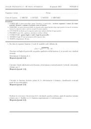
CHAPTER 2. THE 2-DIMENSIONAL CASE: HERMITIAN CURVES2.1. CLASSIFICATION OF INTERSECTIONS IN DIMENSION 2It follows that, for any λ, µ:x(λH + µH ′ )x ⋆ = 0;hence, E ⊆ Γ ∩ . Conversely, since H, H ′ ∈ Γ, if x ∈ Γ ∩ , then x ∈ E and the lemma follows.We may observe that the proof of Lemma 2.1.2 does not require Γ to be the GF( √ q)-linearsystem generated by H and H ′ . In fact, any linear system generated by H and H ′ would do;however, the GF( √ q)-linear system is the largest linear system containing H 1 and H 2 whoseelements are all Hermitian curves. Such a linear system can be seen as a line in the projectivespace PG(n 2 + 2n, √ q) considered as the set of all Hermitian varieties over PG(n, q).Thanks to Lemma 2.1.2, it is sufficient to classify all Hermitian pencils in PG(n, q) in orderto have a description of all possible incidence configurations.For any Hermitian pencil Γ, let r i (Γ) be the number of Hermitian varieties in Γ of rank i.Clearly, the sum of all r i ’s is √ q.Lemma 2.1.3. The cardinality of the intersection of two Hermitian curves H 1 and H 2 dependsonly upon the indices r i (Γ) of the linear system they generate. The possible intersection numbersare as in Table 2.1.r 1 r 2 k = |E|0 3 ( √ q + 1)√ 21 1 q + 10 2 q + √ q + 10 1 q + 11 0 10 0 q − √ q + 1Table 2.1: Possible intersection numbers for non-degenerate Hermitian Curves.This lemma can be found in Kestenband [Kes81]. However, it is a special case of the generalresult of Theorem 4.1.26. The main result of [Kes81] is the following theorem.Theorem 2.1.4. Let H be a non-degenerate Hermitian matrix in Mat(3, q) and let M(x) andC(x) be its minimal and characteristic polynomials. Then, the intersection E of the canonicalHermitian curve U 2 and H(H) belongs to one of the following seven classes.(i) Class I: M(x) = C(x) = (x−α)(x−β)(x−γ) with α, β, γ distinct elements of GF( √ q):• |E| = ( √ q + 1) 2 ;• the points are as in Figure 2.1.a;• r 3 (Γ) = √ q − 2; r 2 (Γ) = 3.38

CHAPTER 2. THE 2-DIMENSIONAL CASE: HERMITIAN CURVES2.1. CLASSIFICATION OF INTERSECTIONS IN DIMENSION 2(ii) Class II: M(x) = H(x) = (x − α)(x − δ) 2 with α, δ distinct elements of GF( √ q):• |E| = q + √ q + 1;• the points are as in Figure 2.1.b;• r 3 (Γ) = √ q − 1; r 2 (Γ) = 2.(iii) Class III: M(x) = C(x) = (x − α)p(x) with p(x) polynomial of degree 2 irreducibleover GF( √ q):• |E| = q + 1;• the points are as in Figure 2.1.c;• r 3 (Γ) = √ q; r 2 (Γ) = 1.(iv) Class IV: M(x) = C(x) = (x − λ) 3 :• |E| = q + 1;• the points are as in Figure 2.1.d;• r 3 (Γ) = √ q; r 2 (Γ) = 1.(v) Class V: M(x) = (x − α)(x − β) with α, β distinct elements of GF( √ q):• |E| = √ q + 1;• the points constitute a Baer subline of PG(2, q);• r 3 (Γ) = √ q − 1; r 2 (Γ) = 1.(vi) Class VI: M(x) = (x − λ) 2 :• |E| = 1;(vii) Class VII:• r 3 (Γ) = √ q; r 2 (Γ) = 0.• |E| = q − √ q + 1;• no three points of E are collinear;• r 3 (Γ) = √ q + 1.Observe that considering only linear systems containing the canonical Hermitian curve U 2does not hamper generality, since it is always possible to reduce to one of those via a projectivity.39

CHAPTER 2. THE 2-DIMENSIONAL CASE: HERMITIAN CURVES2.1. CLASSIFICATION OF INTERSECTIONS IN DIMENSION 2r 1 r 2 M H (x)0 3 (x − α)(x − β)(x − γ)1 1 (x − α)(x − β)0 2 (x − α) 2 (x − β)0 1 (x − α)p(x), (x − α) 31 0 (x − α) 20 0 p(x)Table 2.2: Minimal polynomials corresponding to given rank sequences in the 2-dimensionalcase.2.1.2 Outline of the proofTheorem 2.1.4 is proven by constructing suitable canonical forms for Hermitian matrices inMat(3, q) modulus Hermitian equivalence and considering the various cases arising individually.This is done via the following lemma, which provides ‘canonical’ forms for Hermitianmatrices.Lemma 2.1.5. Let H be a Hermitian matrix in Mat(3, q) and assume M H (x) to be its minimalpolynomial. Then, H is Hermitian equivalent to one of the matrices in Table 2.3.M H (x) conditions canonical form⎡ ⎤α 0 0(x − α)(x − β)(x − γ)⎣ 0 β 0 ⎦⎡0 0 γ⎤α 0 0(x − α)(x − β)⎣ 0 β 0 ⎦⎡0 0 γ⎤α 0 0(x − α)(x − δ) 2 (β − γ) 2 + 4a √ q+1 = 0 ⎣ 0 β a ⎦0 a √ q⎡γ⎤α 0 0(x − α)p(x) (β − α)(γ − α) ≠ a √ q+1 ⎣ 0 β a ⎦0 a √ q⎡γλ c √ ⎤q0(x − λ) 3 a √ q+1 + c √ q+1 = 0 ⎣ c λ a √ q ⎦0 a λTable 2.3: Canonical forms for 3 by 3 Hermitian matrices.In fact, the intersections might be described by just considering the position of two speciallychosen curves in Γ. Since this is the basic tool for the projective classification that we present40

CHAPTER 2. THE 2-DIMENSIONAL CASE: HERMITIAN CURVES2.1. CLASSIFICATION OF INTERSECTIONS IN DIMENSION 2q+1q+1q+1q+12.1.a: ( √ q + 1) 2 points2.1.b: q + √ q + 1 pointsCq +1q-1q+12.1.c: q + 1 pointsq2.1.d: q + 1 pointsFigure 2.1: Possible configurations for the 2-dimensional casein the next section, it is worth to provide here a list of these suitable ‘special’ curves for Γbelonging to the various classes.For any of the classes I-VII, let H be a curve in Γ different from U 2 . Then, H might bechosen as follows:(i) Class I:(ii) Class II:(iii) Class III:• H is a Hermitian cone with vertex not in U 2 ,• each generator of H is a chord of U 2 ;• H is a Hermitian cone with vertex in U 2 ,• each generator of H is a chord of U 2 ;41

CHAPTER 2. THE 2-DIMENSIONAL CASE: HERMITIAN CURVES2.2. GROUPS OF THE INTERSECTION OF TWO HERMITIAN CURVES(iv) Class IV(v) Class V(vi) Class VI(vii) Class VII• H is a Hermitian cone with vertex outside U 2 ,• two generators of H are tangent to U 2 , all the others being chords;• H is a Hermitian cone with vertex in U 2 ,• one generator of H is tangent to U 2 , all the others being chords;• H is a doubly degenerate Hermitian curve, that is a line counted √ q + 1 times,• H is a chord of U 2 ;• H is a doubly degenerate Hermitian curve,• H is tangent to U 2 ;• H is a non-singular Hermitian curve.Definition 2.1.6. A point of the intersection E is special if it is either the vertex of a Hermitiancone in Γ or the only common point of E with a generator of a Hermitian cone in Γ.There are• no special points in classes I, V, VI and VII;• one special point in classes II and IV;• two special points in class III.2.2 Groups of the intersection of two Hermitian curves2.2.1 IntroductionAs presented in Section 2.1, Kestenband’s paper [Kes81] classifies the point-line configurationsarising from the intersection of two Hermitian curves. Nothing is said about projective equivalenceof the configurations in a given class nor about the linear collineation groups preservingthe structures. This is the aim of the present section. This work has been submitted for publicationas [Giub]. I would like to thank Professor G. Korchmáros for helpful discussions on thetopic.42

CHAPTER 2. THE 2-DIMENSIONAL CASE: HERMITIAN CURVES2.2. GROUPS OF THE INTERSECTION OF TWO HERMITIAN CURVESLet H 1 and H 2 be Hermitian curves and denote by E their intersection. As before, let Γ bethe GF( √ q)-linear system generated by H 1 and H 2 and define for any i = 1, 2, 3, the set Γ i asthe subset of Γ which contains all the curves of rank i. Clearly, r i (Γ) = |Γ i |.Our main results are the following theorems.Theorem 2.2.1. Each of the seven classes I-VII consists of pairwise projectively equivalentHermitian intersections.Theorem 2.2.2. The linear collineation group Aut(E) preserving a Hermitian intersection Eacts transitively on both the special and non-special points of E. The abstract structure ofAut(E) depends on the class containing E and is given in Theorems 2.2.9, 2.2.15, 2.2.18, 2.2.22,2.2.24, 2.2.26, 2.2.28.2.2.2 A non-canonical model of PG(2, q)Definition 2.2.3. For any i ≤ j, a projective subspace Π of order p i is in canonical position inPG(n, p j ) if and only ifΠ ∩ PG(n, p j ) = PG(n, p i ),that is, Π is the subspace of PG(n, p j ) coordinatized over GF(p i ).In order to compute the collineation group fixing a Hermitian intersection of class VII, amodel of PG(2, q) that does not lie in canonical position in PG(2, q 3 ) is needed. The resultshere presented are from [CK98] and [CK97].Let F = GF(q), where q = p h and p is odd. Consider the field G = GF(q 3 ) as a cubicextension of F; furthermore take b as a primitive (q 2 + q + 1)-th root of unity over G. The linearcollineation β of PG(2, G) given by⎧⎨ X → bXβ : Y → b q+1 Y⎩Z → Zhas clearly order q 2 + q + 1 and fixes each vertex of the fundamental triangle X ∞ Y ∞ Z ∞ ofPG(2, G).Let B = 〈β〉; the point orbit of E = (1, 1, 1) under B is the setΠ = {(c, c q+1 , 1) : c q2 +q+1 = 1, c ∈ G}.Such a set induces a subgeometry in PG(2, G), whose points are the points of Π and whoselines are the lines of PG(2, G) intersecting Π in at least 2 (and hence in q + 1) points. In fact,this subgeometry is a projective plane, see [CKT99] and [CK98].43

CHAPTER 2. THE 2-DIMENSIONAL CASE: HERMITIAN CURVES2.2. GROUPS OF THE INTERSECTION OF TWO HERMITIAN CURVESTheorem 2.2.4 ([CK98], Proposition 1). The subgeometry Π is isomorphic to PG(2, F). Moreprecisely, Π is a projective subplane of PG(2, E) lying in non-classical position. The lines of Πhave equation [tx + t q+1 y + z = 0], with t running on the (q 2 + q + 1)-th roots of unity and theyform the line-orbit of [x + y + z = 0] under the group B.It can be proven, see [CKT99], that the collineation⎧⎨ X → bX + Y + b q2 +1 Zκ : Y → b⎩q2 +1 X + bY + ZZ → X + b q2 +1 Y + bZmaps PG(2, q) into Π. Observe that β is a Singer cycle of Π which is represented in diagonalform.In order to simplify the notation, the symbol (i) will be used to denote the point (b i , b i(q+1) , 1)of Π. Similarly, [i] will indicate the line of Π of equation [b i X + b i(q+1) Y + Z = 0].2.2.3 Equations for the non-singular Hermitian curveThere is only one non-singular Hermitian curve up to projectivities in PG(2, q); however, whendescribing intersection configurations, it is useful to have different models for the curves. Table2.4 presents the standard equations that will be used.(M1) X √ q+1 + Y √ q+1 + Z √ q+1 = 0(M2) X √ q+1 + Y Z √q + Y √q Z = 0(M3) XY √q − X √q Y + ωZ √ q+1 = 0 ω √ q−1 = −1(M4) XY √q + Y Z √q + ZX √q = 0Table 2.4: Equations for the non-degenerate Hermitian curveAll the models (M1)-(M3) of the Hermitian curve are GF(q)-equivalent, that is, there existsa linear transformation in PGL(3, q) that maps one equation into the other.The model (M1) is the one induced by the canonical Hermitian form and corresponds tothe identity matrix. Equations (M2) and (M3) allow to consider easily the affine points of theHermitian curve H: in (M2), the line at infinity l ∞ : [Z = 0] is tangent to H at the pointY ∞ = (0, 1, 0); in (M3), the polar of the point Z ∞ = (0, 0, 1) is the line l ∞ and the intersectionbetween l ∞ and H is a subline belonging to PG(2, √ q) ⊆ PG(2, q).Let H be the curve in the plane Π corresponding to the equation (M4). We want to provethat H is a Hermitian curve.Lemma 2.2.5. The stabiliser of H in the group B is a subgroup K of order q− √ q+1 generatedby β (q+√ q+1) .44

CHAPTER 2. THE 2-DIMENSIONAL CASE: HERMITIAN CURVES2.2. GROUPS OF THE INTERSECTION OF TWO HERMITIAN CURVESProof. The mapping β transforms the equation of HH : XY √q + Y Z √q + ZX √q = 0intoH β : (b q√ q+q+2 √ q+1 )[XY √q + Y Z √q + ZX √q ] = 0;hence, the group K stabilises H. Conversely, suppose that β l stabilises H. Then,The result follows.b (q√ q+q+1)l = b (q+1)l = b √ ql .Lemma 2.2.6. The set H is a Hermitian curve of Π.Proof. We prove that H is a classical unital. First, we verify that the mapping{ √ (i) → [iq q]ϕ :[i] → (iq √ q)is a non-degenerate polarity. Since Π is a cyclic plane, it is enough to show that ϕ sends linesthrough (0) to points incident with [0] and vice-versa. The line [i] is incident with the point(0) if and only if b i + b i(q+1) + 1 = 0 that is b iq√q + b i(q+1)q√q + 1 = 0. As (iq √ q) is theimage point of [i], the first assertion follows. A similar argument proves the converse. A directcomputation shows also that the set of all self-conjugate points of ϕ coincides with H. Theclassification of polarities of PG(2, q) implies that the polarity ϕ is either orthogonal or unitary.Hence, in order to get the result, it remains to prove that the former possibility cannot actuallyoccur. It is well known, see Lemmas 1.7.43 and 1.7.44, that the set of all self-conjugate pointsof an orthogonal polarity is a (non-degenerate) conic for q odd and a line for q even. On theother hand, no collineation group preserving either a conic or a line contains a cyclic subgroupof order q − √ q + 1. Hence, Lemma 2.2.5 rules out the possibility for ϕ not to be unitary.It follows that the model (M4) is not GF(q)-equivalent to (M1); however it is GF(q 3 )-equivalent.2.2.4 Groups preserving the intersection of two Hermitian curvesLet Aut(E) denote the linear collineation group preserving the Hermitian intersection E of H 1and H 2 . As a subgroup of PGL(3, q), the group Aut(E) acts in a natural way as a permutationgroup on the set of all Hermitian curves in the linear system Γ. More precisely, the three(possibly empty) subsets Γ i ⊆ Γ are invariant under the action of Aut(E).Our approach to computing Aut(E) is to take H 1 from Γ 3 and H 2 from Γ 1 or from Γ 2 , whenΓ 1 is empty, and determine its subgroup G consisting of all linear collineations preserving both45

CHAPTER 2. THE 2-DIMENSIONAL CASE: HERMITIAN CURVES2.2. GROUPS OF THE INTERSECTION OF TWO HERMITIAN CURVESH 1 and H 2 . This will be done by using several properties of the linear collineation groupPSU(3, q) including the classification of all maximal subgroups of PSU(3, q), see [Har26],[Hof72], [Mit11].The subgroup G turns out to be quite large and always transitive on the set of all nonspecialpoints of E. Finally, in order to obtain the whole Aut(E) we will also need some directcomputations depending on the particular properties of E and the possible actions of Aut(E) onthe pencil Γ.Class ILet E be a Hermitian intersection in class I. A non-singular Hermitian curve H 1 in the pencil Γcan be assumed in its canonical form (M1),H 1 : X √ q+1 + Y √ q+1 + Z √ q+1 = 0.Since the collineation group preserving H 1 acts transitively on the points outside H 1 , a Hermitiancone in Γ can be assumed to have its vertex V in the origin O = (0, 0, 1). In particular,both H 1 and H 2 are associated to a diagonal matrix, and this holds true for every curve in thepencil. Under these assumptions, the three Hermitian cones in Γ are of the form1. H 2 : λX √ q+1 + Y √ q+1 = 0;2. H 3 : (λ − 1)Y √ q+1 + λZ √ q+1 = 0;3. H 4 : (1 − λ)X √ q+1 + Z √ q+1 = 0;with λ ∈ GF( √ q) ⋆ \ {1}. A priori, the properties of E may depend on λ. However, as thenext Theorem 2.2.7 states, different choices of λ provide projectively equivalent Hermitianintersections.Theorem 2.2.7. Hermitian intersections in class I are projectively equivalent.Proof. Let λ, ¯λ ∈ GF( √ q) ⋆ \ {1}. Then, there are elements u, v ∈ GF(q) ⋆ such thatu √ q+1 = λ − 1¯λ − 1 ,v√ q+1 =(λ − 1)¯λ(¯λ − 1)λ .Let γ be the linear collineation represented by the non-singular matrix⎡u 0⎤0g = ⎣ 0 v 0 ⎦ .0 0 1The projectivity γ sends H 2 and H 3 to the Hermitian cones of equations ¯λX √ q+1 + Y √ q+1 = 0and (¯λ − 1)Y √ q+1 + ¯λZ √ q+1 = 0. This proves the theorem.46

CHAPTER 2. THE 2-DIMENSIONAL CASE: HERMITIAN CURVES2.2. GROUPS OF THE INTERSECTION OF TWO HERMITIAN CURVESOur next aim is to determine the abstract structure and the action of Aut(E) on the point-set.To do this, the following lemma is needed.Lemma 2.2.8. The collineation group G which preserves both the curve H 1 and the cone H 2consists of all collineationswith ɛ √ q+1 = η √ q+1 = 1. In fact,t(ɛ, η) : (X, Y, Z) → (ɛX, ηY, Z),G ≃ C √ q+1 × C √ q+1,and it acts on the point-set of E as a regular permutation group.Proof. The linear collineations t(ɛ, η) preserve both the curves H 1 and H 2 . In fact,t(ɛ, η)(H 1 ) =(ɛX) √ q+1 + (ηY ) √ q+1 + Z √ q+1 = X √ q+1 + Y √ q+1 + Z √ q+1 =H 1 ;likewise t(ɛ, η)(H 2 ) = H 2 . To show the converse, let γ be a linear collineation of PG(2, q)preserving both H 1 and H 2 . Since γ fixes the vertex (0, 0, 1) of the Hermitian cone H 2 , thenon-singular unitary matrix associated to γ is a block diagonal matrixwith b = c √q . Sinceλ(aX + bY ) √ q+1 + (cX + dY ) √ q+1 =⎡⎣a b 0c d 00 0 1T[(λ(a √q b) + c √q d)X √q Y ] + (λb √ q+1 + d √ q+1 )Y √ q+1 + (λa √ q+1 + c √ q+1 )X √ q+1 ,the condition on γ to preserve H 2 yields(i) b(λa √q + d) = 0;(ii) (λa √ q+1 + b √ q+1 ) = λ(λb √ q+1 + d √ q+1 ) ≠ 0.From (i), we have either b = 0 or b ≠ 0 and d = −λa √q . In the latter case,⎤⎦ ,b √ q+1 = −λa √ q+1and λa √ q+1 + b √ q+1 = 0, against (ii). This shows that b = 0. Then, (ii) implies a √ q+1 = d √ q+1 .Also, from c √ q+1 = b = 0 it follows that c = 0. Hence, the collineation γ is indeed t(a, b) andG ≃ C √ q+1 × C √ q+1.47

CHAPTER 2. THE 2-DIMENSIONAL CASE: HERMITIAN CURVES2.2. GROUPS OF THE INTERSECTION OF TWO HERMITIAN CURVESNote that E = H 1 ∩ H 2 has no point on the fundamental triangle of PG(2, q). On the otherhand, the group G does not fix any point outside the fundamental triangle. It follows that theG-orbit of a point P ∈ H 1 ∩ H 2 has size ( √ q + 1) 2 , the same as G and E. Hence, since E ispreserved by G, E coincides with the orbit of P under G, and G acts regularly.Theorem 2.2.9. The linear collineation group Aut(E) preserving a Hermitian intersection inclass I acts transitively on the points of E. Furthermore, Aut(E) has order 3( √ q + 1) 2 andProof. For any b, c, d ∈ GF(q) such thatAut(E) ≃ (C √ q+1 × C √ q+1) ⋊ S 3 .b √ q+1 = − 1 λ , c√ q+1 = −the group Σ ∼ = S 3 generated by the linear collineations(1 − λ)2, d √ q+1 = λ(1 − λ),λσ 1 : (X, Y, Z) → (Z, dX, cY ),σ 2 : (X, Y, Z) → (bY, b −1 X, Z)is a subgroup of the normaliser of G in Aut(E). In fact, 〈G, Σ〉 = G ⋊ Σ: all collineations inG fix the curves in the pencil Γ; hence, G ∩ Σ = 1. Furthermore, Σ preserves Γ 2 , that is the set{H 2 , H 3 , H 4 } and, in particular, Σ is a subgroup of Aut(E). To show that 〈G, Σ〉 = Aut(E), letτ ∈ Aut(E). Since Σ induces the full symmetric group on Γ 2 , there exists σ ∈ Σ such that στpreserves each of the Hermitian cones H 2 , H 3 , and H 4 . By virtue of the fact that the verticesof these Hermitian cones are also the vertices of the fundamental triangle, it turns out that στ isassociated to a diagonal matrix⎡⎣η 0 00 µ 00 0 1As στ fixes H 2 , we have η √ q+1 = µ √ q+1 . Also, µ √ q+1 = 1, because στ fixes H 3 as well. Thisshows that στ ∈ G, whence Aut(E) = 〈G, Σ〉. The claim now follows from the above resultstogether with Lemma 2.2.8.⎤⎦ .Class IILet E be a Hermitian intersection in class II. A non-singular Hermitian curve H 1 in the pencilΓ is assumed in the canonical form (M2),H 1 : X √ q+1 + Y Z √q + ZY √q = 0,while a Hermitian cone with vertex Y ∞ = (0, 1, 0), sayH 2 : λX √ q+1 + Z √ q+1 = 0,48

CHAPTER 2. THE 2-DIMENSIONAL CASE: HERMITIAN CURVES2.2. GROUPS OF THE INTERSECTION OF TWO HERMITIAN CURVESis chosen to generate Γ together H 1 . One more Hermitian cone belongs to Γ, namelyH 3 : λY Z √q + λZY √q − Z √ q+1 = 0.Its vertex is the point at infinity X ∞ = (1, 0, 0).Theorem 2.2.10. Hermitian intersections in class II are projectively equivalent.Proof. Let Γ and ¯Γ be two pencils which define Hermitian intersections belonging to class II,and let Γ = 〈H 1 , H 2 〉. Without loss of generality, we may assume that ¯Γ is generated by H 1together with the Hermitian cone of equation¯λX √ q+1 + Z √ q+1 = 0,where ¯λ ∈ GF( √ q) ⋆ . Arguing as in the proof of Theorem 2.2.7, choose an element u ∈ GF(q) ⋆such that u √ q+1 = λ/¯λ. The linear collineationξ : (X, Y, Z) → (uX, u √ q+1 Y, Z).sends H 2 and H 3 to the Hermitian cones of equations ¯λX √ q+1 + Z √ q+1 = 0 and ¯λY Z √q +¯λZY √q − Z √ q+1 = 0, whence the claim follows.We now determine the structure and the action on E of the linear collineation group Aut(E)preserving E. By Theorem 2.2.10, we may assume without loss of generality λ = −1. Hence,the vertex of H 3 is the point Y ∞ = (0, 1, 0).Lemma 2.2.11. A linear collineation γ belongs to Aut(E) if and only ifwith(i) d ∈ GF( √ q) ⋆ ;(ii) T(c) = 1 − d;(iii) N[a] = d 2 .γ(a, c, d) : (X, Y, Z) → (aX, Y + cZ, dZ),Proof. The collineation γ fixes the vertices (1, 0, 0) and (0, 1, 0) of both Hermitian cones in Γ.Hence, it is represented by a non-singular matrix of the form⎡a 0⎤bg = ⎣ 0 1 c ⎦ .0 0 dSince γ preserves H 2 ,γ(H 2 ) = λ(aX + bZ) √ q+1 + (dZ) √ q+1 =λa √ q+1 X √ q+1 + (b + d) √ q+1 Z √ q+1 + T[ab √q XZ √q ] = H 2 .Hence, given that a ≠ 0, the following are necessary conditions for g in order to represent γ:49

CHAPTER 2. THE 2-DIMENSIONAL CASE: HERMITIAN CURVES2.2. GROUPS OF THE INTERSECTION OF TWO HERMITIAN CURVES(i) b = 0;(ii) a √ q+1 = d √ q+1 .On the other hand, the image of H 3 under γ isγ(H 3 ) = λ[T((Y + cZ)(dZ) √q ] − (dZ) √ q+1 =λT[d √q Y Z √q + cd √q Z √ q+1 ] − (dZ √ q+1 ) =λT[d √q Y Z √q ] + (T[cd √q ] − d √ q+1 )Z √ q+1 .Hence, d ≠ 0 and γ(H 3 ) = H 3 , which together imply d √q = d, that is (i), and dT[c] − d 2 = d,that is (ii).Lemma 2.2.12. Let G be the subgroup of Aut(E) preserving H 1 . Then, we can write Aut(E) =C √ q−1G, where C √ q−1 is the cyclic group consisting of all collineationswith d ∈ GF( √ q) ⋆ .φ(d) : (X, Y, Z) → (X, Y, dZ)Proof. The action on H 1 of a collineation γ which is represented by a matrix g as in Lemma2.2.11 is as follows:γ(H 1 ) = d 2 X √ q+1 + dT[Y Z √q ] + T[c]Z √ q+1 .In order for the image to be H 1 , we clearly need d = 1 and T[c] = 0. The latter yields N[a] = 1;hence, every element in Aut(H) can be written as a the product of an element in C √ q−1 by anelement in G.Lemma 2.2.13. The group G has order ( √ q + 1) √ q and it is isomorphic to the semidirectproduct of an elementary Abelian normal subgroup of order √ q by a cyclic group of order√ q + 1.Proof. The collineations γ(1, c, 1) form an elementary Abelian subgroup E √ q of order √ q.Likewise, the set of the collineations of the form γ(a, 0, 1) with N[a] = 1 constitutes a cyclicsubgroup C √ q+1 of order √ q + 1. The generic element of G is of the form g(a, c, 1), with thebefore mentioned conditions on c and a. In fact,which implies the result.g(a, c, 1) = g(1, c, 1)g(a, 0, 1),Lemma 2.2.14. The group G acts on the points of E distinct from (0, 1, 0) as a regular permutationgroup.50

CHAPTER 2. THE 2-DIMENSIONAL CASE: HERMITIAN CURVES2.2. GROUPS OF THE INTERSECTION OF TWO HERMITIAN CURVESProof. We keep using the notation introduced in the previous lemma. Let ∆ 2 be the set ofall generators of H 2 . The cyclic component C √ q+1 consists of elations of centre X ∞ and axis[X = 0]. Since [X = 0] is not an element of ∆, but C √ q+1 preserves H 2 , we obtain that C √ q+1acts in a fixed-point free manner on ∆. It follows that C √ q+1 is regular on the generators ofH 2 . Likewise, the elementary Abelian subgroup E √ q of G acts transitively on the set of allgenerators ∆ 3 of H 3 distinct from [Z = 0]. Since any point of E is obtained as the intersectionof an element of ∆ 2 with an element of ∆ 3 , it follows that G is transitive on the points of Edistinct from (0, 1, 0). Finally, observe that G has order √ q( √ q + 1) which is equal to the sizeof E \ (0, 1, 0).By virtue of the above lemmas, both the abstract structure and the action of Aut(E) arecompletely determined.Theorem 2.2.15. The linear collineation group Aut(E) preserving a Hermitian intersectionE in class II acts transitively on the points of E distinct from the special point. Furthermore,Aut(E) has order √ q(q − 1) andClass IIIAut(E) ≃ C √ q−1 × (E √ q ⋊ C √ q+1).Let E be a Hermitian intersection in class III. A non-singular Hermitian curve H 1 in the pencilΓ is assumed to be in form (M3), that isH 1 : XY √q − X √q Y + ωZ √ q+1 = 0,with ω √ q−1 = −1. Since the collineation group preserving H 1 is doubly transitive on the pointsof H 1 , the two generators of the Hermitian cone H 2 in E may be assumed to be the tangent linesto H 1 at the points (0, 1, 0) and (1, 0, 0). Then, H 2 has equationH 2 : XY √q − uY X √q = 0,with u √ q+1 = 1. Actually, u ≠ 1. In fact, every generator of H 2 different from the axes mustbe a chord of H 1 , and this occurs if and only if u ≠ 1. Hence, in our setting, we have just √ qpairwise distinct Hermitian intersections.Theorem 2.2.16. Hermitian intersections in class III are projectively equivalent.Proof. For every t ∈ GF (q) such that u = t √ q−1 , define the linear collineationThe image of H 1 under θ t isθ t : (X, Y, Z) → ((1 − t) −1 X, Y, Z).θ t (H 1 ) = (1 − t) −1 XY √q − (1 − t √q ) −1 X √q Y + ωZ √ q+1 := ¯H 1 .51

CHAPTER 2. THE 2-DIMENSIONAL CASE: HERMITIAN CURVES2.2. GROUPS OF THE INTERSECTION OF TWO HERMITIAN CURVESLikewise,θ t (H 2 ) = (1 − t) −1 XY √q − u(1 − t √q ) −1 Y X √q = XY √q + X √q Y.On the other hand, since H 1 = ¯H 1 +t(t−1) −1 ¯H2 , the collineation θ t maps E into the Hermitianintersection Ē generated by H 1 and ¯H 2 . For two distinct values of t, the resulting Hermitianintersections do not coincide. In fact, if t ∈ GF(q) also satisfies the above condition, that is¯t √ q−1 = u, and (1−t)(1−t √q ) −1 = (1− ¯t)(1− ¯t) √ q−1 holds, then we have (1−t)(1−tu) −1 =(1−¯t)(1−u¯t) −1 , and the latter relation implies t = ¯t. This shows that the family parametrized byt consists of √ q − 1 pairwise distinct Hermitian intersections which are projectively equivalentto E. None of them coincides with E, as (1 − t)(1 − t √q ) = 1 implies u = 1 which is currentlyruled out. Adding E to that family, we obtain all possible Hermitian intersections, and thiscompletes the proof.To determine the abstract structure and the action of Aut(E), we need some further preliminaryresults.Lemma 2.2.17. The linear collineation group G preserving both H 1 and H 2 consists of allcollineationsγ(a) : (X, Y, Z) → (a √ q+1 X, Y, aZ),δ(a) : (X, Y, Z) → (−a √ q+1 Y, X, aZ),with a ∈ GF(q) ⋆ . The subgroup H = {γ(a)|a ∈ GF(q) ⋆ } is a cyclic normal subgroup ofG, and it acts regularly on the points of E distinct from (1, 0, 0) and (0, 1, 0). Furthermore, ifa ∈ GF( √ q) ⋆ and q is even, then δ(a) is an involution and G = 〈δ(a)〉 ⋊ H; if q is odd, thenδ(a) has order 4 and G = C 2 ⋊ H.Proof. Let g be a linear collineation preserving both H 1 and H 2 . Then, g preserves the fundamentaltriangle. More precisely, g fixes the origin Z ∞ = (0, 0, 1) and either interchangesthe points Y ∞ = (0, 1, 0) and X ∞ = (1, 0, 0), or fixes them both. In the former case, g isrepresented by a diagonal non-singular matrix⎡M 1 (a, b) = ⎣b 0 00 1 00 0 aThe collineation g preserves H 2 if and only if GF ( √ q) ⋆ contains b. For b ∈ GF ( √ q) ⋆ , thecondition on g to preserve H 1 is equivalent to a √ q+1 = b. Hence, if g fixes the vertices of thefundamental triangle, then g = γ(a) with a suitable element a ∈ GF ( √ q) ⋆ . A similar argumentshows that if g interchanges the vertices X ∞ and Y ∞ , then g is represented by the non-singularmatrix⎡M 2 (a, b) = ⎣520 b 01 0 00 0 a⎤⎦ .⎤⎦ ,

CHAPTER 2. THE 2-DIMENSIONAL CASE: HERMITIAN CURVES2.2. GROUPS OF THE INTERSECTION OF TWO HERMITIAN CURVESand a necessary and sufficient condition for g to preserve both H 1 and H 2 is b = −a √ q+1 . Thiscompletes the proof of the first statement. The group H is isomorphic to the multiplicativegroup of GF(q); hence, it is cyclic of order q − 1. Since δ(b) −1 γ(a)δ(b) = γ(a √q ) for alla, b ∈ GF (q) ⋆ , the group H is normal in G. As no non-trivial element in the subgroup H fixesa point outside the fundamental triangle, the orbit of any point P ∈ E under H has size q − 1,the same as E. It follows that the orbit of a P ∈ E is the whole of E. This completes the proofof the second statement.By direct computation, the square of δ isδ(a) 2 : (X, Y, Z) → (−a √ q+1 X, −a √ q+1 Y, a 2 Z).Hence, when q is even, for any a ∈ GF( √ q) ⋆ , the collineation δ(a) is an involution and G =〈δ(a)〉⋊H. When q is odd, δ(a) has period 4, but δ(a) 2 = γ(−1) ∈ H; hence, G = C 2 ⋊H.We are in position to prove the following theorem.Theorem 2.2.18. The linear collineation group Aut(E) preserving a Hermitian intersection Ein class III acts transitively on the points of E distinct from the two special points. Furthermore,Aut(E) has order 2(q − 1) andAut(E) ≃ C 2 ⋊ C q−1 .Proof. We prove that every linear collineation g preserving E belongs to the group G introducedin the previous lemma. Actually, g preserves H 2 ; hence, it suffices to prove that g also preservesH 1 . As we have already noticed in the proof of Lemma 2.2.17, the condition on g to preserveH 2 implies that g is represented by either one of the matrices M 1 (a, b) or M 2 (a, b), with a ∈GF (q) ⋆ , b ∈ GF ( √ q) ⋆ . In the former case, g sends H 1 to the Hermitian curve ¯H 1 of equationXY √q − X √q Y + (a √ q+1 b −1 )ωZ √ q+1 = 0.On the other hand, the pencil Γ generated by H 1 and H 2 contains ¯H 2 if and only if a √ q+1 b −1 =1. This only occurs for b = a √ q+1 , that is for g ∈ G. A similar argument shows that the sameholds when g is represented by M 2 (a, b).Class IVLet E be a Hermitian intersection in class IV. The non-singular Hermitian curveH 1 : X √ q+1 + Y Z √q + Y √q Z = 0given by the model (M2), together with the Hermitian cone H 2 of vertex (0, 1, 0) and equationcan be chosen to generate the pencil Γ.H 2 : ZX √q − λXZ √q = 0, λ √ q+1 = 153

CHAPTER 2. THE 2-DIMENSIONAL CASE: HERMITIAN CURVES2.2. GROUPS OF THE INTERSECTION OF TWO HERMITIAN CURVESTheorem 2.2.19. Hermitian intersections in class IV are projectively equivalent.Proof. Let λ, ¯λ be elements of GF(q) with λ √ q+1 = ¯λ √ q+1 = 1. Choose a ∈ GF(q) ⋆ such thata √ q−1 = (¯λ/λ). Arguing as in the proof of Theorem 2.2.10, it suffices to check that the linearcollineationγ(a) : (X, Y, Z) → (aX, Y, Z)preserves H 1 and sends H 2 to the Hermitian cone ¯H 2 of equation¯H 2 : ZX √q − ¯λXZ √q = 0.The previous lemma guarantees that in order to determine Aut(E) we may assume withoutloss of generality λ = 1.Lemma 2.2.20. The collineation group G which preserves both H 1 and H 2 consists of allcollineations⎧⎨ X → aX + cZt(a, c, f) : Y → −acX + a 2 Y + fZ⎩Z → Z,with a ∈ GF( √ q) ⋆ , c ∈ GF( √ q) and T[f] = −N[c].Proof. Via a direct computation, we havet(H 1 ) = a 2 X √ q+1 + a 2 T[Y Z √q ] + (c 2 + f)Z √ q+1 ,t(H 2 ) = aH 2 .Hence, any collineation t(a, c, f) belongs to G. Conversely, let γ be a linear collineation preservingH 2 . Then, γ is an elation of centre (0, 1, 0) and axis [Z = 0]. It follows that γ isassociated to a non-singular matrix⎡⎣a 0 cd e f0 0 1with a ∈ GF( √ q) ⋆ and c ∈ GF( √ q). Since γ preserves H 1 as well, then d = −ac, e = a 2 andT[f] = −N[c].Lemma 2.2.21. The subgroup T of G consisting of all collineations of the form t(1, 0, f) iselementary Abelian of order √ q. In fact, T ≃ E √ q, and G/T ≃ AGL(1, √ q). The group T isthe translation subgroup of G.⎤⎦ ,54

CHAPTER 2. THE 2-DIMENSIONAL CASE: HERMITIAN CURVES2.2. GROUPS OF THE INTERSECTION OF TWO HERMITIAN CURVESProof. The order of t(1, 0, f) is, for any suitable f, equal to the characteristic p of GF( √ q) andany two elements in T commute; hence, T is an elementary Abelian group. Since T(f) = 0has √ q solutions, T has order √ q and T ≃ E √ q. Let now Ḡ be the permutation group inducedby G on the set ∆ of all generators of H 2 . We show that the kernel K of the permutationrepresentation G → Ḡ is T . It is immediate to verify that any element of T fixes all the linesthrough (0, 1, 0); hence, T ≤ K. On the other hand, the generic line through (0, 1, 0) is of theforml : [αZ + X] = 0,with α ∈ GF(q) ∪ {∞}. Any linear collineation t of G acts on l by transforming it into the linel t : [(α + c)Z + X] = 0.aHence, if a ≠ 1 or c ≠ 0, the collineation t(a, c, f) fixes at most two generators of H 2 . It followsthat T is the full kernel of the representation of G into Ḡ. The proof is completed by observingthat, according to Lemma 2.2.20, Ḡ acts on ∆ as the group of all permutations X → aX + cwith a ≠ 0 and c ranging over GF( √ q).The abstract structure and the action of the linear collineation group Aut(E) are given in thefollowing theorem.Theorem 2.2.22. The linear collineation group Aut(E) preserving a Hermitian intersection Ein class IV acts transitively on the points of E distinct from the special point. Furthermore,| Aut(E)| = q( √ q − 1) andAut(E)/E √ q ≃ AGL(1, √ q).Proof. The translation group T acts transitively on the common points of E and any affineline through (0, 1, 0). Also, as seen in the proof of the previous lemma, G acts transitivelyon the generators of H 2 . This proves the transitivity of G on the points of E distinct from(0, 1, 0). It remains to show that G coincides with Aut(E). Take g ∈ Aut(E) and let ḡ be thepermutation induced by g on the set ∆ of the generators of H 2 . If g is in the kernel of thepermutation representation Aut(E) → Aut(E), then g is a translation. Let T ′ = 〈T, g〉 be thegroup generated by T and g. Then, T ′ is again a translation group. Hence, no non-trivial elementin T ′ fixes an affine point. On the other hand, T ′ preserves the set of all common points of Eand one affine line through (0, 1, 0). This yields that T ′ has order at most √ q; hence T ′ = T ,that is g ∈ T . The factor group Aut(E)/T induces on ∆ a permutation group containing G/T .Since Aut(E)/T preserves H 2 , it follows that Aut(E)/T consists of permutationsX → aX + b,with a ∈ GF( √ q) ⋆ , b ∈ GF( √ q). This proves that G/T = Aut(E)/T and, therefore, G =Aut(E).55

CHAPTER 2. THE 2-DIMENSIONAL CASE: HERMITIAN CURVES2.2. GROUPS OF THE INTERSECTION OF TWO HERMITIAN CURVESClass VIILet E be a Hermitian intersection in class VII. Then, [BS86], [Cos97], [Ebe85], [FHT86] and[Kes89] have proven that E is the point-orbit of a Singer subgroup of order (q − √ q + 1) and itspoints form a complete (q − √ q + 1)-arc in PG(2, q). In this case, we will use the model (M4)for H 1 :H 1 : XY √q + Y Z √q + ZX √q = 0.Observe that the collineation β maps the curve H associated with the equation (M4) into theHermitian curve of equationH β 1 : b q√ q+1 XY √q + b q−√ q+1 Y Z √q + ZX √q = 0.Since H 1 ≠ H β , we may choose H β as H 2 . The intersection E = H 1 ∩ H β 1 consists of thepoints of Π that satisfy the following system of equations:It follows that⎧⎨⎩XY √q + Y Z √q + ZX √q = 0(a q−√ q+1 − a q√ q+1 )Y Z √q + (1 − a q√ q+1 )ZX √q = 0Z = 1.Y = −X √ q aq2 +q+1 − a q√ q+1a q−√ q+1− a q√ q+1 = X√ q aq(q−√ q+1) − 1a √ q(q− √ q+1− 1 = X√q (a (q−√ q+1 − 1) q−1 = X √q .Hence, E is represented by all the points of the form (ɛ, ɛ √q , 1) with ɛ q−√ q+1 = 1 and it is a setof cardinality q − √ q + 1. From 2.1.4, it follows that E is an arc and that the intersection of H 1and H 2 = H β 1 is in class VII.Theorem 2.2.27. Hermitian intersections in class VII are projectively equivalent.Proof. This theorem is a corollary to the known result that any two Singer subgroups of thesame order are conjugate under the full linear collineation group PGL(3, q) of PG(2, q), see[Blo67], [Har26] and [Mit11].Theorem 2.2.28. The linear collineation group Aut(E) preserving a Hermitian intersection Ein class VII is transitive on the points of E. Furthermore, Aut(E) contains a normal cyclicsubgroup of order q − √ q + 1 acting regularly on the points of E andAut(E) = C 3 ⋊ C q−√ q+1 .Proof. In the above model, the Singer subgroup S of order q− √ q+1 generated by γ = β q+√ q+1preserves E, as it preserves both H 1 and H 2 . The same holds true for the linear collineationgroup E of order 3 generated byτ : (X, Y, Z) → (Y, Z, X).57

CHAPTER 2. THE 2-DIMENSIONAL CASE: HERMITIAN CURVES2.3. A GROUP-THEORETIC CHARACTERIZATION OF HERMITIAN CURVES ASCLASSICAL UNITALSSince E normalises S, the group G = 〈E, S〉 is the semidirect product of S by E. Hence,G ≃ C 3 ⋊ C q−√ q+1 .To prove that Aut(E) = G it will be useful to regard E as a (q − √ q + 1)-arc. Let Λ be thealgebraic envelope associated to E, viewed as an algebraic curve in the dual plane of PG(2, q).Clearly, Aut(E) is an automorphism group of Λ. For q even, Λ is a projectively equivalentto a non-singular Hermitian curve H, see [Tha87]. The same holds for q odd, provided thatprojective equivalence is replaced by birational equivalence, see [CK98]. In any case, Aut(E)turns out to be isomorphic to a subgroup L of PGU(3, q). Since G ≤ Aut(E), L contains asubgroup isomorphic to G. Then, the assertion follows from the classification of all maximalsubgroups of PGU(3, q), see [Har26], [Hof72] and [Mit11]. In fact, the subgroups of PGU(3, q)which are the semidirect product of a cyclic group of order 3 by a cyclic group of order q− √ q+1are all maximal in PGU(3, q).2.3 A group-theoretic characterization of Hermitian curvesas classical unitalsThe non-canonical model presented in 2.2.2 is used in order to provide a short proof of analready known characterization of classical unitals [CEK00]. This work has been submitted forpublication [Giua].2.3.1 IntroductionWe recall some basic definitions. A unital in a Desarguesian projective plane PG(2, q) of squareorder q, is a set U of q √ q +1 points such that any line of PG(2, q) meets U in either 1 or √ q +1points. The absolute points of a unitary polarity of PG(2, q) form a unital which is calledthe classical (or Hermitian) unital. The linear collineation group of PG(2, q) preserving aclassical unital is PGU(3, q). By a theorem due to Hoffer [Hof72] this group-theoretic propertycharacterises classical unitals: if a unital U is preserved by a collineation group isomorphicto PSU(3, q), then U is classical. Cossidente, Ebert and Korchmáros [CEK00] showed thatHoffer’s result holds true under some weaker assumption, namely for unitals preserved by aSinger subgroup of PGL(3, q) of order q − √ q + 1. Their proof heavily depends on previousresults concerning cyclic partitions of PG(2, q) in Baer sub-planes. A different and shorterproof of this result is the purpose of the present section.Theorem 2.3.1. A unital U in PG(2, q) is classical if and only if it is preserved by a cycliclinear collineation group of order q − √ q + 1.2.3.2 A result on classical unitalsThe following remarkable property of classical unitals is from [CEK00].58

CHAPTER 2. THE 2-DIMENSIONAL CASE: HERMITIAN CURVES2.3. A GROUP-THEORETIC CHARACTERIZATION OF HERMITIAN CURVES ASCLASSICAL UNITALSTheorem 2.3.2 (Proposition 3.2 [CEK00]). Let q = p k . Every unital U of the projective planePG(2, q) meets every classical unital in r ≡ 1 mod p points.Proof. Let l 1 , . . . , l r be a set of lines of PG(2, q) and let ¯l i be the characteristic vector of l i . Bydefinition of unital, a line l intersects U in either 1 or √ q + 1 points. Let ū be the characteristicvector of U. Then, the dot product between ū and any combination of lines can be evaluated asū · (¯l 1 + . . . + ¯l r ) ≡ r mod p.A theorem due to Blokhuis, Brouwer and Wilbrink [BBW91] (see also [AK92, 6.7.1]), statesthat a classical unital H is a codeword in the GF(p)-code generated by the lines of PG(2, q).This is to say that the characteristic vector ¯h of H is a combination of characteristic vectors¯l1 , . . . , ¯l r of the lines of the projective space. Since the number of points of H is q √ q + 1,working modulus p,1 = ¯h · ¯h= ¯h · (¯l 1 + . . . ¯l r )= ¯h · ¯l 1 + . . . ¯h · ¯l r ,and r ≡ 1 mod p. Now, the dot product between ū and ¯h can be computed asThe result follows.ū · ¯h = ū · (¯l 1 + . . . + ¯l r ) = ū · ¯l 1 + . . . + ū · ¯l r ≡ r mod p.2.3.3 Proof of Theorem 2.3.1Here, we consider a Singer collineation group acting on the points and lines of the non-canonicalmodel Π of PG(2, q) in PG(2, q 3 ) as introduced in section 2.2.2.Assume H to be the Hermitian curve of Π with equation (M4) and define K as its stabiliserin B. Since B is Abelian, K is normal in B and it is possible to construct a quotient incidencestructure Π 0 in the following way: define thick points as the point-orbits of Π under K, thicklines as the orbits of H under B, and incidence as inclusion. Note that the factor group B/Kis a Singer group for Π 0 , as it acts regularly on the set of thick-points as well as on the set ofthick-lines.We need the following characterization of finite projective planes as incidence structures.Lemma 2.3.3 (Proposition 3.2.3(m), [Dem68]). An incidence structure (P, L, I) is a projectiveplane of order n if and only if(i) |P | ≤ n 2 + n + 1;(ii) |L| ≥ n 2 + n + 1;59

CHAPTER 2. THE 2-DIMENSIONAL CASE: HERMITIAN CURVES2.3. A GROUP-THEORETIC CHARACTERIZATION OF HERMITIAN CURVES ASCLASSICAL UNITALS(iii) every line in L contains at least n + 1 points;(iv) any two distinct lines of L meet in at most 1 point.Lemma 2.3.4. The incidence structure Π 0 is a projective plane of order √ q.Proof. Since the index [B : K] is equal to q + √ q + 1, the number of thick-points in Π 0 isq + √ q + 1. According to Lemma 2.2.5, the subgroup of B which preserves H is K; hence, wehave q + √ q + 1 thick lines as well. Furthermore, every thick line is incident with √ q + 1 thickpoints, as the size of H is q √ q + 1. By Lemma 2.3.3, in order to prove that Π 0 is a projectiveplane of order √ q, it now suffices to verify that two thick lines share at most one thick point.Since thick-lines are classical unitals, for q > 9 the assertion follows from the fact that thenumber of common points of two distinct classical unitals in Π is at most ( √ q + 1) 2 , smallerthan 2(q − √ q + 1). For q = 4, 9 a direct counting argument proves the assertion.We are now in position to prove Theorem 2.3.1.Proof of Theorem 2.3.1. For any n | q 2 + q + 1, all Singer subgroups of order n are conjugatein P GU(3, q); hence, we may assume without loss of generality that U is a unital in Π whichis preserved by K. This hypothesis implies that U is the union of √ q + 1 point-orbits under K,and hence, the unital U can be viewed as a set ∆ of √ q + 1 thick points in Π 0 . In order to proveTheorem 2.3.1, it remains to show that ∆ is actually a thick line, or, equivalently, that U meetsH and every image of H under the action of B; this is a corollary of Theorem 2.3.2.60

Chapter 3The 3-dimensional case: HermitiansurfacesThis chapter deals with the point-line-plane incidence configurations arising from the intersectionof two Hermitian surfaces. First, we consider which intersections fulfill some combinatorialconditions in order to be possible. Later, we determine classes of matrices that allow us to directlyconstruct such intersections. For the purposes of this chapter, we mean by Hermitiancone a degenerate Hermitian surface of rank 3.3.1 Description of incidence configurations in dimension 3In this section we describe the possible point-line configurations arising from the intersectionof two Hermitian surfaces in PG(3, q). The argument here is purely combinatorial. For adescription of the geometric cases which can actually be realized in PG(3, q) and models of theintersections, please see section 3.3.The following result, which will be proven in Chapter 4 for dimension n, is needed.Lemma 3.1.1. Let H 1 , H 2 be two distinct Hermitian surfaces; then, the size of the intersectionE = H 1 ∩ H 2 depends only upon the number and rank of the degenerate surfaces in the linearsystem Γ = 〈H 1 , H 2 〉. Define as r i the number of surfaces in Γ of rank i; then, the size of E forthe various possible values of r i is as in Tables 3.1, 3.2 and 3.3.Definition 3.1.2. A linear system Γ is non-degenerate if it contains at least a non-degenerateHermitian surface.Definition 3.1.3. We say that two points are conjugate with respect to the linear system Γ ifthey are conjugate with respect to any non-degenerate surface in Γ.61

CHAPTER 3. THE 3-DIMENSIONAL CASE: HERMITIAN SURFACES3.1. DESCRIPTION OF INCIDENCE CONFIGURATIONS IN DIMENSION 3r 1 r 2 r 3 k = |E|0 0 0 (q + 1) 20 0 1 (q + √ q + 1)(q − √ q + 1)0 0 2 (q 2 + 1)0 0 3 q 2 − q + 10 0 4 (q − 1) 20 1 0 q 2 + q √ q + q + 10 1 1 q 2 + q √ q + 10 1 2 ( √ q + 1)(q √ q − q + 1)0 2 0 ( √ q + 1)(q √ q + q − √ q + 1)1 0 0 q √ q + q + 11 0 1 q √ q + 1Table 3.1: Possible intersection numbers for Hermitian surfaces: non-degenerate pencil.r 1 r 2 r 3 k = |E|√0 0 q + 1 q 2 − q √ q + q + 1√ √ √0 1 q (q + q + 1)(q − q + 1)√ √0 2 q − 1 ( q + 1) 2 (q − √ q + 1)√0 3 q − 2 q 2 + 2q √ q + √ q + 1√1 0 q q + 1√ √1 1 q − 1 q q + q + 1Table 3.2: Possible intersection numbers for Hermitian surfaces: degenerate pencil; r 30, r 4 = 0.≠r 1 r 2 k = |E|√0 q + 1 2q 2 + q + 1√1 q q 2 + q + 1√2 q − 1 q + 1Table 3.3: Possible intersection numbers for Hermitian surfaces: degenerate pencil; r 20, r 3 = r 4 = 0.≠62

CHAPTER 3. THE 3-DIMENSIONAL CASE: HERMITIAN SURFACES3.1. DESCRIPTION OF INCIDENCE CONFIGURATIONS IN DIMENSION 33.1.1 Some general remarks on conesLemma 3.1.4. Assume r 3 (Γ) ≥ 1 and r 4 (Γ) ≥ 1. Take a cone C of vertex V in Γ. Let π be thepolar plane of V with respect to a non-degenerate surface H ∈ Γ, and define k = |C ∩ H| andh = |P| whereP := C ∩ H ∩ π.Then, if V ∉ H,if V ∈ H,k = q 2 + q √ q + √ q + 1 − √ qh;k = q 2 + √ q + 1 + (h − 1)( √ q − 1 √ q).Proof. All tangents to the surface H through V are of the form V P with P ∈ π ∩ H; hence, allcomponents of the cone C tangent to H are of the form V P ′ with P ′ ∈ P, while the remaining(q √ q + 1 − h) lines are secant, that is intersecting H in √ q + 1 distinct points.Hence,k = h + (q √ q + 1 − h)( √ q + 1),and the first part of the lemma is proven.Assume now that V ∈ H. This implies that V ∈ π and π is tangent to H. Hence, π ∩ Hdecomposes in √ q + 1 lines. On the other hand, π intersects C in either one point or in aHermitian cone, that is in √ q + 1 lines. Let j = (h − 1)/q be the number of lines of π incommon between C and H. Each of these lines is fully included in H ∩ C. All lines of C not onπ are secant to H, that is they intersect H in √ q + 1 points, one of those is V . It follows,k = √ q(q √ q + 1 − j) + 1 − jq,that isk = q 2 + √ q + 1 + (h − 1)( √ q − 1 √ q).Corollary 3.1.5. Assume C to be a Hermitian cone of vertex V ∉ H and let π be the polar planeof V . As usual, denote by r i the number of Hermitian surfaces of rank i in the linear system Γ.Then, the intersection between C and H belongs to one of the classes presented in table 3.4.Proof. The proof is done directly by a counting argument.Corollary 3.1.6. Assume that r 1 (Γ) = r 2 (Γ) = 0, while r 3 (Γ), r 4 (Γ) ≥ 1, and let C 1 and C 2 bedistinct cones in Γ of vertices respectively V 1 and V 2 . If V 2 ∉ E, then V 1 belongs to the polarplane π of V 2 with respect to any non-degenerate surface in Γ.63

CHAPTER 3. THE 3-DIMENSIONAL CASE: HERMITIAN SURFACES3.1. DESCRIPTION OF INCIDENCE CONFIGURATIONS IN DIMENSION 3h r 1 r 2 r 3 |U 3 ∩ K| (r ′ 1, r ′ 2)q − √ q + 1 0 0 1 q 2 + q + 1 (0, 0)q + 1 0 0 2 q 2 + 1 (0, 1)q + √ q + 1 0 0 3 q 2 − q + 1 (0, 2)( √ q + 1) 2 0 0 4 q 2 − 2q + 1 (0, 3)1 0 1 1 q 2 + q √ q + 1 (1, 0)√ q + 1 0 1 2 q 2 + q √ q − q + 1 (1, 1)q √ q + 1 1 0 1 q √ q + 1 N.A.Table 3.4: Possible intersections E between a cone and a non degenerate Hermitian surface;vertex not in the intersection.The column (r ′ 1, r ′ 2) describes the type of planar configuration in E ∩ π, where π is the polarplane of the vertex of C.Proof. Let π be the polar plane of V 2 with respect to a non-degenerate surface H ∈ Γ. Considerthe line l = V 1 V 2 . If V 1 ∉ π, then l intersects E = C 1 ∩ C 2 in either √ q + 1 or q + 1 points, butV 2 ∉ E implies that the intersection in q + 1 points is not possible. On the other hand, a linethrough the vertex of a cone intersects the cone in either 1 or q + 1 points – a contradiction. Itfollows that V 1 ∈ π.Corollary 3.1.7. Let C 1 and C 2 be two Hermitian cones in a non-degenerate linear system Γ.Assume that the parameters of Γ are of the form (0, r 2 , r 3 ), and let π be the polar plane of thevertex of C 2 with respect to any non-degenerate surface in Γ. Then, the intersection Σ of C 1 withπ is a curve of a class corresponding to the parameters (r 2 , r 3 − 1).Proof. The claim follows from the observation that π ∩ C 1 is a degenerate curve. By looking upthe orders in Table 2.1 we complete the proof.Lemma 3.1.8. The configurations given by Σ are uniquely determined up to projectivities bythe rank sequence (r 1 , r 2 , r 3 ).Proof. From Theorem 2.2.1, all plane intersections determining the same point-line configurationare projectively equivalent. Furthermore, following [Kes81], we see that a point-lineconfiguration is uniquely determined by its cardinality k except in the case (r ′ 1, r ′ 2) = (0, 1),when k = q + 1.The case k = q + 1, corresponds to the situation in which Γ contains a cone C whosevertex V does not belong to E and the rank sequence is (0, 0, 2). A priori, there would be twopossibilities for E ∩ π:(i) the intersection consists of √ q − 1 sublines, all disjoint;(ii) the intersection consists of q sublines, all with a point in common.64

CHAPTER 3. THE 3-DIMENSIONAL CASE: HERMITIAN SURFACES3.1. DESCRIPTION OF INCIDENCE CONFIGURATIONS IN DIMENSION 3In both cases, the lines containing the points of the intersection belong also to the cone of thepencil whose vertex V ′ is in the polar plane π of V . On the other hand, in case (ii), such vertexV ′ has to belong to H as well and the size of E would have to be q 2 + q + 1, while, from Table3.4, we already know |E| = q 2 + 1; a contradiction. It follows that the surfaces intersect in π inthe configuration given by (i).Lemma 3.1.9. Let Γ be a non-degenerate pencil of Hermitian surfaces and assume that thereis at least a cone C in Γ whose vertex V does not belong to the base locus E. Then, the verticesof any other cone in Γ belong to the polar plane π of V with respect to any non-degeneratesurface H ∈ Γ.Proof. The intersection of E with π corresponds to the configuration obtained as base locusof a pencil of Hermitian curves with parameters (r ′ 1, r ′ 2) = (r 2 , r 3 − 1). Hence, for r 3 ≥ 2,the section of any cone C ′ ∈ Γ different from C with the plane π is a set of √ q + 1 lines, allconcurrent in a point V ′ ∈ π. It follows that V ′ has to be the vertex of C ′ .3.1.2 Pencils whose degenerate surfaces have all rank 3In this subsection we describe the possible incidence configurations E when the pencil Γ isassumed to contain only cones as degenerate surfaces.The vertex of any cone C i ∈ Γ is denoted with the letter V i . By H we denote, as usual, ageneric non-degenerate surface in Γ.For any cone C ∈ Γ, the indices s i are defined in Table 3.5.s 1s 2number of components of C which are included in Enumber of components of C which are chords of Es 3 number of components of C tangent to E.Table 3.5: Indices for the intersection of a cone and a Hermitian surface.Lemma 3.1.10. Assume that Γ contains 4 cones C 1 , . . . , C 4 . Then, for any i = 1, . . . , 4, V i ∉ E;furthermore, all components of any cone C i intersect E in √ q + 1 points.Proof. The cardinality of E is (q −1) 2 . Assume that the vertex of a cone C 1 in Γ does not belongto E. Then, each line of C 1 intersects H in either √ q + 1 or 1 points. Hence,(q − 1) 2 = s 2 ( √ q + 1) + (q √ q + 1 − s 2 );this is equivalent to say that there are s 2 = q √ q − q − 2 √ q lines of C 1 which are chords of Eand q + 2 √ q + 1 lines which are tangent to E. Furthermore, since this configuration contain noline, the vertex of none of the cones in Γ may belong to E.65

CHAPTER 3. THE 3-DIMENSIONAL CASE: HERMITIAN SURFACES3.1. DESCRIPTION OF INCIDENCE CONFIGURATIONS IN DIMENSION 3Assume now that the vertex V of C belongs to Γ. Then,(q − 1) 2 − 1 = s 1 (q) + s 2 ( √ q) + (q √ q − s 1 − s 2 ).This would yieldq(q − √ q − 1) = ( √ q − 1)[s 1 ( √ q + 1) + s 2 ],a contradiction, since s 1 and s 2 are both natural numbers and ( √ q − 1) does not divide q(q −√ q − 1). The result follows.Lemma 3.1.11. Assume that Γ contains exactly 3 distinct cones and assume also that there isat least a cone C ∈ Γ whose vertex V is not in E. Then, √ q(q − √ q − 1) components of C arechords of H; furthermore, any cone in Γ whose vertex is in E contains q √ q − 1 chords and 2tangents to H.Proof. Since V is not in H, thenq 2 − q + 1 = s 2 ( √ q + 1) + (q √ q − s 2 + 1).Hence,q[q − √ q − 1] = s 2 ( √ q)and s 2 = √ q(q − √ q − 1) components of C are chords of H; the remaining q + √ q + 1components are tangent to the surface. On the other hand, if C ′ is a cone of Γ whose vertexbelongs to H, thenq 2 − q + 1 = s ′ 1(q) + s ′ 2( √ q) + 1.Hence,√ q(q − 1) = (√ q)s′1 + s ′ 2.The result follows now by observing that V ∉ H implies s ′ 1 = 0.Lemma 3.1.12. Let Γ be a pencil with r 3 (Γ) ≥ 2. Assume that the vertices V 1 , V 2 of any twocones C 1 , C 2 in Γ belong to E; then, the line V 1 V 2 is included in E.Proof. The line V 1 V 2 intersects E in at least two points. Since Γ is generated by C 1 and C 2 , thisimplies that V 1 V 2 is a component of both C 1 and C 2 . The result follows.Lemma 3.1.13. Assume r 3 (Γ) = 3, r 4 (Γ) ≥ 0. Then, either the vertex of at most one cone of Γbelongs to E or the vertices of all three cones in Γ lie on the same line in E.Proof. Assume that the vertices V 1 and V 2 of two cones C 1 and C 2 of Γ are points of E. Then,according to Lemma 3.1.12, the line V 1 V 2 has to be included in E as well, and s ′ 1 = 1. On theother hand, C 1 and C 3 generate Γ and the only lines completely in C 3 are those through V 3 . Thelemma follows.66

CHAPTER 3. THE 3-DIMENSIONAL CASE: HERMITIAN SURFACES3.1. DESCRIPTION OF INCIDENCE CONFIGURATIONS IN DIMENSION 3Lemma 3.1.14. Let r 3 (Γ) = 3 and assume r 4 (Γ) ≥ 0. Then, E contains one line and √ q(q −2)sublines.Proof. From the previous lemma, s ′ 1 = 1. Hence,The result follows.q 2 − q + 1 = (q + 1) + s ′ 2( √ q).Lemma 3.1.15. Assume r 3 (Γ) = 2. Then, one of conditions (i)-(iii) has to be satisfied.Proof. Let C be a cone of Γ with vertex V .If V ∉ E, thenq 2 + 1 = s 2 ( √ q + 1) + (q √ q + 1 − s 2 ).Hence,Hence,If V ∈ H, thenIt follows that there are three possibilities:s 2 = (q √ q − q).q 2 = s 1 (q) + s 2 ( √ q).s 2 = √ q(q − s 1 ).(i) the vertex of both cones in Γ belongs to E; then, s 1 = s ′ 1 = 1 and s ′ 2 = s 2 = q √ q − 1;(ii) the vertex of a cone in Γ belongs to E, the other not; then, s 1 = 0, s 2 = q( √ q − 1) ands ′ 2 = q √ q;(iii) the vertex of none of the cones in Γ belongs to H; then, s 2 = s ′ 2 = q( √ q − 1).Lemma 3.1.16. Assume that r 3 (Γ) = 1 and let C be the only cone in the pencil. If the vertexV of C does not belong to E, then √ q[q − √ q + 1] lines of C are chords; if V ∈ E, then theconfiguration E contains at least a line.Proof. If the vertex V of C does not belong to H, thenHence,If the vertex V of C belongs to H, thenq 2 + q + 1 = s 2 ( √ q + 1) + (q √ q + 1 − s 2 ).s 2 = √ q[q − √ q + 1].q 2 + q + 1 = s 1 (q) + s 2 ( √ q) + 1;hence, s 2 = √ q(q + 1 − s 1 ). Since in this case s 2 ≤ q √ q + 1, it follows s 1 ≥ 1. On the otherhand, since s 1 ∈ {1, √ q + 1}, we obtain s 2 ∈ {q √ q, q √ q − q}.67

CHAPTER 3. THE 3-DIMENSIONAL CASE: HERMITIAN SURFACES3.1. DESCRIPTION OF INCIDENCE CONFIGURATIONS IN DIMENSION 3Class c 3 v s ′ 1 s ′ 2 s 2 ka 4 0 - - q √ q + 1 (q − 1) 2b 3 0 - -√ √ q(q − q − 1) q 2 − q + 1c 3 1 0√ q(q − 1)√ √ q(q − q − 1) q 2 − q + 1d 3 3 1√ q(q − 2)√ √ q(q − q − 1) q 2 − q + 1e 2 0 - - q( √ q − 1) q 2 + 1f 2 1 0 q √ q q( √ q − 1) q 2 + 1g 2 2 1 q( √ q − 1) - q 2 + 1h 1 0 - -√ √ q(q − q + 1) q 2 + q + 1k-I 1 1 1 q √ q - q 2 + q + 1k-II 1 1 2√ q(q − 1) - q 2 + q + 1k-III 1 1√ q + 1√ q( q − 1) - q 2 + q + 1Table 3.6: Possible incidence classes for two non-degenerate Hermitian surfaces: Γ containsdegenerate surfaces of rank 3 only.Table 3.6 presents all possible incidence configurations obtained as base locus of linearsystems Γ whose only degenerate surfaces are Hermitian cones. The first column contains thetotal number c 3 of cones in a given configuration. The number v is the number of cones in thepencil Γ whose vertex belongs to the intersection. The numbers s 1 and s 2 are as in Table 3.5 fora cone C whose vertex does not belong to E. The integers s ′ 1 and s ′ 2 are defined in the same wayfor a cone C ′ whose vertex is assumed to be in E.3.1.3 Pencils whose degenerate surfaces have all rank 2This subsection deals with the case in which all degenerate surfaces in the linear system Γ haverank 2, that is to say r 3 (Γ) = r 1 (Γ) = 0. We recall that the radical of a Hermitian form h is theset of the points x of PG(n, q) such that for all y ∈ PG(n, q),h(x, y) = 0.Definition 3.1.17. The radical of a Hermitian surface H is the radical of the Hermitian form hassociated with H. We denote the radical of H with the symbol rad H.Lemma 3.1.18. The radical of a Hermitian variety H is a subspace of PG(n, q). Furthermore,the following equality holds:dim rad H + rankH = n.68

CHAPTER 3. THE 3-DIMENSIONAL CASE: HERMITIAN SURFACES3.1. DESCRIPTION OF INCIDENCE CONFIGURATIONS IN DIMENSION 3Proof. Consider the linear transformation φ induced by H. We have, dim ker φ+dim Im φ = n;on the other hand, dim ker φ = dim rad H and dim Im φ = rankH. The result follows.Lemma 3.1.19. Assume that the only degenerate surface C of Γ has rank 2; then, the radical ofC intersects any non-degenerate surface H ∈ Γ in either 1, √ q + 1 or q + 1 points.Proof. Any plane which is a component of C, intersects H in either a Hermitian curve or in a degenerateHermitian curve, that is √ q+1 lines through a point. In the former case the intersectionconsists of q √ q + 1 points; in the latter of q √ q + q + 1. Define v 1 as the number of componentsof C which intersect H in a degenerate curve and let v 2 be the number of components secant toH, that is, whose intersection is a non-singular curve. Obviously, v 1 + v 2 = √ q + 1.Since C has rank 2, its radical l = rad C is a line of PG(3, n). Hence, the possible intersectionnumbers with H are 1, √ q + 1 or q + 1. Let n = |l ∩ H|. We now analyse allpossibilities.Class I.a: n = 1. The size of E isq 2 + q √ q + q + 1 = v 1 (q √ q + q) + ( √ q + 1 − v 1 )q √ q + 1.We obtain v 1 = 1.Class I.b: n = √ q + 1. The size of E isq 2 + q √ q + q + 1 = v 1 (q √ q + q − √ q) + ( √ q + 1 − v 1 )(q √ q − √ q) + √ q + 1 =Hence, v 1 = 2.Class I.c: l = q + 1. The size of E isq 2 + q √ q + q + 1 = v 1 (q √ q) + ( √ q + 1 − v 1 )(q √ q − q) + q + 1.Hence,and v 1 = (1 + √ q).q 2 + q √ q = v 1 q + q 2 − qCorollary 3.1.20. Let Γ be a non-degenerate linear system of Hermitian surfaces with r 2 (Γ) =2. Assume C and C ′ to be the two degenerate surfaces in Γ. Then, the radicals of C and C ′ areskew.Proof. Assume V to be a point in the intersection of the radicals of C and C ′ . Then, V isconjugate to any point of PG(3, q) with respect to the Hermitian form induced by a linearcombination of C and C ′ . It follows that V is in the radical of any surface of Γ, a contradiction.Lemma 3.1.21. Let Γ, C and C ′ be as in corollary 3.1.20. Then, all components of the degeneratesurfaces C and C ′ are secant to all the non-degenerate surfaces of Γ. Furthermore, theradical of C is contained in a component of C ′ and vice-versa.69

CHAPTER 3. THE 3-DIMENSIONAL CASE: HERMITIAN SURFACES3.1. DESCRIPTION OF INCIDENCE CONFIGURATIONS IN DIMENSION 3Class c 2 v p 1 p 2 kI-a 1 1 1√ q q 2 + q √ q + q + 1I-b 1√ q + 1 2√ q − 1 q 2 + q √ q + q + 1I-c 1 q + 1√ q + 1 0 q 2 + q √ q + q + 1II-c 2 q + 1 0√ q + 1 q 2 + 1Table 3.7: Possible incidence classes for two non-degenerate Hermitian surfaces: Γ containsdegenerate surfaces of rank 2 only.Proof. Let n be the size of the intersection of the radical of C with a non-degenerate surfaceH ∈ Γ. Then, n is either 1, √ q + 1 or q + 1. We now analyse the different possibilities.Class II.a: n = 1. Then,a contradiction.Class II.b: n = √ q + 1. Then,a contradiction.Class II.c: n = q + 1. Then,q 2 + 1 = v 1 q + q 2 + q √ q + 1 > q 2 + 1,q 2 + 1 = v 1 q + ( √ q + 1)(q − 1) √ q + √ q + 1q 2 + q = v 1 q + q(q − 1) + q + 1 = v 1 + q 2 + 1.This case is actually possible and yields v 1 = 0. It follows that all components of C are secantto any non-degenerate surface H.Table 3.7 presents all possible incidence classes E for two Hermitian surfaces H 1 , H 2 whenthe pencil they generate contains degenerate surfaces of rank 2 only.Here, the second column contains the total number c 2 of degenerate surfaces in a givenconfiguration; v is the number of points in common between the radical of a degenerate surfaceand the intersection configuration E.We recall that a plane π is tangent E if it is tangent to any non-degenerate surface in Γ; wesay that π is secant (or transversal to) E if it intersects a non-degenerate surface of Γ in a nonsingularHermitian curve. By p 1 , the number of planes, components of a degenerate surface inΓ, that are tangent E is denoted; p 2 is the number of planes in such a surface that are secant E.70

CHAPTER 3. THE 3-DIMENSIONAL CASE: HERMITIAN SURFACES3.1. DESCRIPTION OF INCIDENCE CONFIGURATIONS IN DIMENSION 33.1.4 Pencils whose degenerate surfaces have ranks 2 and 3This subsection describes the configurations E arising from the intersection of two Hermitiansurfaces, when the non-degenerate pencil Γ they generate is assumed to contain both Hermitiancones and doubly-degenerate Hermitian surfaces; that is to say that both r 2 (Γ) ≠ 0 and r 3 (Γ) ≠0. We assume that C 1 ∈ Γ is a degenerate surface of rank 2 and that C 2 ∈ Γ has rank 3. Thesymbols in Table 3.8 will be used. Observe that the indices s 1 , s 2 and s 3 are not independent.In fact, since C 2 is a cone over a non-degenerate Hermitian curve, s 1 + s 2 + s 3 = q √ q + 1.s 1s 2s 3v 1v 2components of C 2 included in Ecomponents of C 2 secant to (being chords of) Ecomponents of C 2 tangent to Eplanes of C 1 tangent to Eplanes of C 1 secant to El 1 intersection between rad C 1 and C 2l 2 intersection between rad C 2 and C 1Table 3.8: Indices for the intersection of Hermitian surfaces of rank 2 and of rank 3.Lemma 3.1.22. Assume that a non-degenerate linear system Γ contains a surface C 1 ∈ Γ ofrank 2 and a surface C 2 ∈ Γ of rank 3. Then, the vertex of C 2 does not belong to the radical ofC 1 . Furthermore, the components of C 1 and C 2 intersect H as illustrated in Table 3.9, Class I.Proof. Since C 1 ≠ C 2 , the surfaces C 1 and C 2 generate the linear system Γ. On the other hand,Γ is non-degenerate by assumption; hence, the vertex of C 2 cannot belong to the radical of C 1 .This proves the first part of the lemma.We distinguish some different cases. First, we consider the information obtained by consideringthe intersection between the lines of C 2 and E. There are two possibilities:Class I.a: V 2 ∉ E. Then, s 1 = 0 andq 2 + q √ q + 1 = s 2√ q + q√ q + 1.Hence, s 2 = q √ q and the intersection between the polar plane of the vertex of C 2 and E ∩ C 2consists of a single point.Class I.b: V 2 ∈ E. Then,q 2 + q √ q + 1 = s 1 q + s 2√ q + 1.Hence, s 1√ q + s2 = q √ q + q, with s 1 + s 2 ≤ q √ q + 1. This implies s 2 = √ q(q + √ q − s 1 ) andq + √ q + 1 > s 1 > √ q. On the other hand, the lines shared between C 2 and E must lie in the71

CHAPTER 3. THE 3-DIMENSIONAL CASE: HERMITIAN SURFACES3.1. DESCRIPTION OF INCIDENCE CONFIGURATIONS IN DIMENSION 3tangent plane τ at V to any non-degenerate surface H in Γ. Hence, they lie in the intersectionof the 2-dimensional cone C 2 ∩ τ with the cone H ∩ τ. Such an intersection contains either 0,1, 2 or √ q + 1 lines. It follows s 1 = √ q + 1, s 2 = q − 1 and s 3 = q √ q − q − √ q + 1.Now we focus on the intersection between the plane components of C 1 and H. Let l 1 be thecardinality of the intersection between the radical of C 1 and E. There are three actual possibilities:Class I.i: l 1 = 1. Then,q 2 + q √ q + 1 = v 1 (q √ q + q) + ( √ q + 1 − v 1 )(q √ q) + 1.Hence, v 1 = 0 and v 2 = √ q+1, that is all the components of C 1 are secant to any non-degeneratesurface H.Class I.ii: l 1 = √ q + 1. Then,q 2 + q √ q + 1 = √ q[v 1 (q + √ q − 1) + ( √ q + 1 − v 1 )(q − 1) + 1] + 1.Hence, v 1 = 1, v 2 = √ q and one of the components of C 1 is tangent to any non-degeneratesurface H.Class I.iii: l 1 = q + 1. Then,Hence, v 1 = √ q and v 2 = 1.q 2 + q √ q + 1 = q[v 1 ( √ q) + ( √ q + 1 − v 1 )( √ q − 1) + 1] + 1.Lemma 3.1.23. Let Γ be a linear system of Hermitian surfaces such that r 3 (Γ) = 2 and r 2 (Γ) =1. Take C 2 and C 3 as the Hermitian cones of Γ and assume C 1 to be the doubly-degeneratesurface in the linear system. Define r as the radical line of C 1 . Then, either the vertices of bothC 2 and C 3 belong to E, or none of them does.Proof. Let l 1 = |E ∩ r|.There are two possible classes with respect to the components of one of the cones, say C 2 :Class II.a: V 2 ∉ E. Then,Hence, s 2 = √ q(q − 1).Class II.b: V 2 ∈ E. Then,q 2 + q √ q − q + 1 = s 2 ( √ q + 1) + (q √ q + 1 − s 2 ).q 2 + q √ q − q + 1 = s 1 q + s 2√ q + 1.If s 1 = 0, then s 2 = q √ q + q − √ q > q √ q + 1, impossible. Hence, s 1 = 1 and the vertex of C 3has to belong to E as well. Furthermore, s 2 = q √ q − √ q.72

CHAPTER 3. THE 3-DIMENSIONAL CASE: HERMITIAN SURFACES3.2. HERMITIAN MATRICES AND POLYNOMIALSIn fact, the intersection between the components of C 1 and E can be realized in only twoways, since most of the possibilities are ruled out by considerations on the order.Class II.i: l 1 = 1. Then,q 2 + q √ q − q + 1 = v 1 (q √ q + q) + ( √ q + 1 − v 1 )(q √ q) + 1;hence, v 1 = −1, a contradiction, since v 1 ≥ 0.Class II.ii: l 1 = √ q + 1 Then,q 2 + q √ q − q + 1 = √ q[v 1 (q + √ q − 1) + ( √ q + 1 − v 1 )(q − 1) + 1] + 1;hence, v 1 = 0.Class II.iii: l 1 = q + 1 points. Then,hence, v 1 = √ q and v 2 = 1.q 2 + q √ q − q + 1 = q[v 1 ( √ q) + ( √ q + 1 − v 1 )( √ q − 1)] + 1;3.1.5 Pencils with r 1 (Γ) ≥ 1A Hermitian surface of rank 1 is a plane π repeated √ q+1 times. The intersection configurationE associated to a linear system Γ with r 1 (Γ) = 1 is hence planar. In fact, a plane might meet anon-degenerate Hermitian surface H in only two configurations:(i) Class III-a: π is tangent to H; the intersection E is a Hermitian cone, that is a Hermitiancurve of rank 2;(ii) Class III-b: π is secant to H; the intersection E is a non-degenerate Hermitian curve.From Table 3.1, we have that in Class III-a, the rank sequence (r 1 , r 2 , r 3 ) for Γ is (1, 0, 0); inClass III-b, (r 1 , r 2 , r 3 ) = (1, 0, 1) and there is a cone C in Γ whose vertex does not belong to π.3.2 Hermitian matrices and polynomialsIn this section, we provide some matrices which represent classes of Hermitian intersections.This is useful in order to construct the possible intersection configurations in dimension 3.The results are presented in Tables 3.10, 3.11, 3.12.73

CHAPTER 3. THE 3-DIMENSIONAL CASE: HERMITIAN SURFACES3.2. HERMITIAN MATRICES AND POLYNOMIALSClass c2 c3 l2 l3 s1 s2 v1 kI-a-i 1 1 1 0 0 q √ q 0 q 2 + q √ q + 1√ √I-a-ii 1 1 q + 1 0 0 q q 1 q2 √ + q q + 1I-a-iii 1 1 q + 1 0 0 q √ √q q q2 √ + q q + 1√I-b-i 1 1 1 1 q + 1 q − 1 0 q2 √ + q q + 1√ √I-b-ii 1 1 q + 1 1 q + 1 q − 1 1 q2 √ + q q + 1√ √I-b-iii 1 1 q + 1 1 q + 1 q − 1 q q2 √ + q q + 1√ √II-a-ii 1 2 q + 1 0 0 q(q − 1) 1 q2 √ + q q − q + 1√ √II-a-iii 1 2 q + 1 0 0 q(q − 1) q q2 √ + q q − q + 1√ √II-b-ii 1 2 q + 1 1 + 1 1 q(q − 1) 1 q2 √ + q q − q + 1√ √II-b-iii 1 2 q + 1 1 + 1 1 q(q − 1) q q2 √ + q q − q + 1Table 3.9: Possible incidence classes for two non-degenerate Hermitian surfaces: Γ containsdegenerate surfaces of ranks 2 and 3.74

CHAPTER 3. THE 3-DIMENSIONAL CASE: HERMITIAN SURFACES3.2. HERMITIAN MATRICES AND POLYNOMIALSMH(x) conditions canonical form⎡⎤(x − α)(x − β)(x − γ) 2 (η − ξ) 2 + 4c √ q+1 = 0See Lemma 3.2.7α 0 0 0⎢ ⎢⎣ 0 β 0 00 0 η c √ q+10 0 c ξ⎡⎤⎥ ⎥⎦(x − α)(x − β)(x − γ)α 0 0 0⎢ ⎢⎣ 0 β 0 00 0 γ 00 0 0 δ⎡⎥ ⎥⎦(x − α)(x − β) 3 c √ √q+1 + d q+1 = 0See Lemma 3.2.8α 0 0 0⎢ ⎢⎣ 0 β c 00 c √ q+1β d √ q+10 0 d β⎡⎤(λ − µ) 2 − 4b √ q+1 = 0(x − α) 2 (x − β) 2 (η − ξ) 2 − 4d √ q+1 = 0See Lemma 3.2.9λ b √ q0 0⎢ ⎢⎣ b µ 0 00 0 η c √ q0 0 c ξ⎡⎤⎥ ⎥⎦(x − α) 2 (x − β)(λ − µ) 2 − 4b √ q+1 = 0See Lemma 3.2.10λ b √ q⎢ 0 0b µ 0 00 0 β 00 0 0 β⎥ ⎥⎦⎤⎥ ⎥⎦Table 3.10: Canonical forms for the 3-dimensional case: M H (x) splits over GF( √ q); 2 or 3distinct roots.75

CHAPTER 3. THE 3-DIMENSIONAL CASE: HERMITIAN SURFACES3.2. HERMITIAN MATRICES AND POLYNOMIALSMH(x) conditions canonical form⎡⎤(x − α)(x − β)(x − γ)(x − δ) See Lemma 3.2.7α 0 0 0⎢ ⎢⎣ 0 β 0 00 0 γ 00 0 0 δ⎥ ⎥⎦⎡α a b cSee Lemmas 3.2.11, 3.2.14(x − α) 4 σ = (ad) √ √q b − (ad)b q⎢ ⎢⎣ a √ qα d eT[(ad) √ q b √ qd √ qα fbσ] ≠ 0c √ qe √ qf √ qα⎡(x − α) 3 See Lemmas 3.2.11, 3.2.14α a b c⎢ ⎢⎣ a √ qα d eb √ qd √ qα fc √ qe √ qf √ qα⎡(x − α) 2 See Lemma 3.2.11α a b c⎢ ⎢⎣ a √ qα d eb √ qd √ qα fc √ qe √ qf √ qα⎤⎥ ⎥⎦⎤⎥ ⎥⎦⎤⎥ ⎥⎦Table 3.11: Canonical forms for the 3-dimensional case: M H (x) splits over GF( √ q); 1 or 4roots.76

CHAPTER 3. THE 3-DIMENSIONAL CASE: HERMITIAN SURFACES3.2. HERMITIAN MATRICES AND POLYNOMIALSMH(x) conditions canonical form⎤(x − α)(x − β)p2(x)α 0 0 0(ξ − ζ) 2 + 4d √ q+1 ∉ □ 0 0 ζ c⎡See Lemma 3.2.16⎢⎢⎣ 0 β 0 00 0 c √ qξ⎡⎥ ⎥⎦(x − α)p3(x)(x − α) 2 p2(x)See Lemma 3.2.17(λ + µ) 2 + 4c √ q+1 = 0(η − α)(ξ − α) ≠ d √ q+1α 0 0 0⎢ ⎢⎣ 0 λ d e0 d √ qη f0 e √ qf √ qξ⎡λ c 0 0⎢ ⎢⎣ c √ qµ d e0 0 η d0 0 d √ qξp2(x)q2(x)⎡λ c 0 cSee Lemma 3.2.18⎢ξ 2 − (λ + µ)ξ + d √ √q+1 − c q+1 ⎢⎣ c √ qµ d e≠ 00 0 η d0 0 d √ qξp2(x) 2 ⎡λ c 0 c⎢ ⎢⎣ c √ qµ d e0 0 η d0 0 d √ qξ⎤⎥ ⎥⎦⎤⎥ ⎥⎦⎤⎥ ⎥⎦⎤⎥ ⎥⎦Table 3.12: Canonical forms for the 3-dimensional case: M H (x) does not split over GF( √ q);degree 4.77

CHAPTER 3. THE 3-DIMENSIONAL CASE: HERMITIAN SURFACES3.2. HERMITIAN MATRICES AND POLYNOMIALS3.2.1 Some general considerations on Hermitian pencilsThis subsection presents some general considerations that will be used later.The first lemma proves that if we want to consider linear systems Σ in which any twovarieties intersect in the same configuration, then the dimension of Σ is at most 1. In the secondlemma, we verify that if the base locus E of a linear system Γ of Hermitian varieties has maximalcardinality, then Γ is a maximal set of Hermitian varieties meeting in E. These results hold forany dimension n.Lemma 3.2.1. Let Σ be a linear system of Hermitian varieties. If any two distinct elements ofΣ meet in the same configuration, then dim Σ = 1.Proof. The set Σ is a projective subspace of PG(n 2 + 2n, √ q). Take three linearly independentHermitian varieties H 1 , H 2 , H 3 ∈ Σ and let H 1 , H 2 and H 3 be corresponding Hermitianmatrices. Assume also thatE := H 1 ∩ H 2 = H 1 ∩ H 3 = H 2 ∩ H 3 .The three varieties H 1 , H 2 , H 3 are all different; if it were H 3 ⊆ H 1 ∪ H 2 , then we could writeH 3 = (H 3 ∩ H 1 ) ∪ (H 3 ∩ H 2 ) = E ∪ E = E = H 1 ∩ H 2 .This is a contradiction, since H 1 ≠ H 2 and E is not a Hermitian variety. Then, there exists at ∈ H 3 \ E, belonging neither to H 1 nor to H 2 . The matrix H ′ given byH ′ = H 1 − ( tH 1t ⋆tH 2 t ⋆ )H 2identifies a Hermitian variety H ′ := H(H ′ ) in the linear system Γ, defined by H 1 and H 2 . Suchvariety H ′ intersects H 3 in t. Again, from the independence of H 3 from H 1 and H 2 ,a contradiction.H ′ ≠ H 3 ,Corollary 3.2.2. Let H 1 , H 2 and H 3 be three independent Hermitian matrices such thatThen, for any µ in GF( √ q),H(H 1 ) ∩ H(H 2 ) = H(H 2 ) ∩ H(H 3 ) = H(H 1 ) ∩ H(H 3 ).H(H 1 ) ∩ H(H 2 ) ⊆ H(H 1 ) ∩ H(H 2 + µH 3 ).78

CHAPTER 3. THE 3-DIMENSIONAL CASE: HERMITIAN SURFACES3.2. HERMITIAN MATRICES AND POLYNOMIALSProof. By hypothesis, we haveH(H 1 ) ∩ H(H 2 ) = H(H 1 ) ∩ H(H 2 ) ∩ H(H 3 ).On the other hand, a solution of the system of equations induced by the three Hermitian matricesH 1 , H 2 and H 3 is necessarily a solution of the system determined by H 1 and H 2 + µH 3 . Theresult follows.Lemma 3.2.3. Assume that two Hermitian varieties H 1 and H 2 intersect in a configurationE of maximal cardinality. Then, the only Hermitian varieties intersecting H 1 in E are thosebelonging to the linear system Γ defined by H 1 and H 2 .Proof. Assume H 3 to be a Hermitian variety intersecting H 1 in E. Because of the maximalityof E, it is also H 3 ∩H 2 = E. Now, Corollary 3.2.2 affirms that any linear combination of H 2 andH 3 intersect H 1 in a superset of E; since E is maximal, such a superset has to be E again. Bythe argument used in the proof of Corollary 3.2.1, this is impossible when H 3 does not belongto Γ, whence the result.Further linear algebra observationsNow we present some linear algebra results. These results are straightforward generalizationsof those in [Kes81].Lemma 3.2.4. Let H and J be two Hermitian matrices equivalent up to unitary transformations.Then, the minimal polynomials M H (x) and M J (x) are the same.Proof. By hypothesis, there exists a matrix U such thatH = UJU ⋆with U ⋆ = U −1 . It follows that H n = (U)J n (U ⋆ ). Hence, for any polynomial p(x) = a 0 +a 1 x + . . . + a n x n such that p(J) = 0,p(H) = a 0 I + a 1 (UJU ⋆ ) + . . . + UJ n U ⋆ = Up(J)U ⋆ = U0U ⋆ = 0.Hence, M H (x) | M J (x). By a similar argument, M J (x) | M H (x) and the result follows.Lemma 3.2.5 ([Kes81], Lemma 3). Let H be a Hermitian matrix and suppose that its minimalpolynomial M H (x) has a factorisationp(x) = p 1 (x)p 2 (x) . . . p k (x)in k > 1 factors co-prime in GF( √ q)[x]. Then, the null spaces corresponding to these factorsare mutually conjugate.79

CHAPTER 3. THE 3-DIMENSIONAL CASE: HERMITIAN SURFACES3.2. HERMITIAN MATRICES AND POLYNOMIALSProof. We work by induction on k. Observe that all p i (x) are Hermitian polynomials, sincetheir coefficients lie in the ground field GF( √ q).Case k = 2: since p 1 (x) and p 2 (x) are co-prime, the Chinese Remainder Theorem impliesthat there exist two Hermitian polynomials r 1 (x), r 2 (x) ∈ GF( √ q)[x] such thathence, the identity matrix I can be written as1 = r 1 (x)p 1 (x) + r 2 (x)p 2 (x);I = r 1 (H)p 1 (H) + r 2 (H)p 2 (H).Assume now v ⋆ ∈ Null H p 1 (x) and w ⋆ ∈ Null H p 2 (x). Then,and, likewise,Hence, H being Hermitian,v = v(p 1 (H)r 1 (H) + p 2 (H)r 2 (H)) = vp 2 (H)r 2 (H)w ⋆ = r 1 (H)p 1 (H)w ⋆ + r 2 (H)p 2 (H)w ⋆ = r 1 (H)p 1 (H)w ⋆ .vw ⋆ = wv ⋆ = w(p 1 (H) ⋆ r 1 (H) ⋆ )v ⋆ = w(r 1 (H)p 1 (H))v ⋆ = wr 1 (H)(p 1 (H)v ⋆ ) = w0 = 0.Induction k ⇒ k + 1: Assume p(x) = p 1 (x) . . . p k+1 (x), and for any 0 < i ≤ k define q i (x)to be p i (x)p i+1 (x). The polynomial q k (x) is co-prime with all the p i (x) for i < k, hence, by theinductive hypothesis, its null space is conjugate with all of theirs. In particular, both the nullspace of p k (x) and that of p k+1 (x) are conjugate with the null space of any other p i (x), sincethey are contained in Null H q k (x). By using the same argument on the factorisation of p(x)given byp(x) = p 1 (x) . . . p k−2 (x)q k−1 (x)p k+1 (x),the null space of p k+1 is proven to be conjugate with the null space of q k−1 , which containsNull H p k (x). The result follows.Lemma 3.2.6. Let H be an n × n Hermitian matrix such that(i) its minimal polynomial M(x) has degree n;(ii) M(x) splits in GF( √ q)[x];(iii) M(x) has no double root.Then, H is unitarily equivalent to a diagonal matrix.80

CHAPTER 3. THE 3-DIMENSIONAL CASE: HERMITIAN SURFACES3.2. HERMITIAN MATRICES AND POLYNOMIALSProof. Consider the matrix U consisting of the representation of H with respect to the baseformed by its normalized eigenvectors. This matrix is diagonal and, by Lemma 3.2.5, is unitarilyequivalent to H, whence the result.We now produce some 4 × 4 Hermitian matrices. These matrices can be (and will be) usedto construct the linear systems corresponding to the cases as presented in section 3.1. CasesI-III assume that the factorisation of the minimal polynomial splits over GF( √ q). Case IVconsiders some of the possibilities when the minimal polynomial of a matrix contains higherdegree irreducible factors.3.2.2 Case I: 3 or 4 distinct rootsLemma 3.2.7. Let H be a 4 × 4 Hermitian matrix whose minimal polynomial has either theform M H (x) = (x − α)(x − β)(x − γ)(x − δ) or M H (x) = (x − α)(x − β)(x − γ). Then, His unitarily equivalent to a diagonal matrix.Proof. The first part of the lemma is a direct consequence of Lemma 3.2.6.Consider now the case in which M H (x) has degree 3 and all its roots are distinct. Thecharacteristic polynomial C H (x) has degree 4 and is divisible by the minimal polynomial of H.It follows that C H (x) splits in linear factors over GF( √ q) as well.Assume the roots of C H (x) not to be the same as those of M H (x). Then,C H (x) = (x − α)(x − β)(x − γ)(x − δ),with α, β, γ and δ all distinct. Clearly, all the matrices (H − αI), (H − βI), (H − γI) and(H − δI) have rank 3; then, M H (H) would have rank 1, a contradiction. It follows thatC H (x) = (x − α)(x − β)(x − γ) 2 .Since α, β and γ are all distinct, the null spaces corresponding to (x − α), (x − β) and (x − γ)are mutually conjugate. Hence, H is unitarily equivalent to a matrix H ′ of the form⎡⎤α 0 0 0H ′ = ⎢ 0 β 0 0⎥⎣ 0 0 σ d ⎦ ,0 0 d θwhere σ, θ ∈ GF( √ q) and d ∈ GF(q). By a direct computation, the characteristic polynomialof H ′ isC H ′(x) = (x − α)(x − β)(x 2 − (σ + θ)x + σθ − d √ q+1 ).On the other hand, C H ′(x) = C H (x); hence, the previous relation implies thatx 2 − (σ + θ)x + σθ − d √ q+1 = (x − γ) 2 ,81

CHAPTER 3. THE 3-DIMENSIONAL CASE: HERMITIAN SURFACES3.2. HERMITIAN MATRICES AND POLYNOMIALSthat is, the following system of equations has to be fulfilled:{ (σ + θ) = 2γσθ − d √ q+1 = γ 2 .This yieldsγ 2 − 2σγ + d √ q+1 + σ 2 = 0;the conclusion is that the norm of d is d √ q+1 = −(γ − σ) 2 . On the other hand, the minimalpolynomial M H ′(x) coincides with the minimal polynomial of H; hence, M H (H ′ ) = 0. Thematrix H ′ is block-diagonal. Assume H ′ = diag(α, β, T ) where T ∈ Mat(2, q), and defineW = M H (T ). Then, we have the following equalities(i) W 1,1 = (γ − σ)[(2γ − σ − α)(2γ − σ − β)+d √ q+1 )] + d √ q+1 (2γ − α − β);(ii) W 1,2 = d[(2γ − σ − α)(2γ − σ − β) + d √ q+1 + (2γ − α − β)(σ − γ)];(iii) W 2,1 = W √ q1,2 ;(iv) W 2,2 = d √ q+1 (γ − α − β + σ) + (σ − α)(σ − β)(σ − γ).A substitution and a simplification in W 1,1 yieldW 1,1 = (γ − σ)(γ − β)(γ − α),whence γ = σ and, consequently, d = 0. It follows that H ′ is diagonal.3.2.3 Case II: 2 distinct rootsLemma 3.2.8. A non-degenerate 4 × 4 Hermitian matrix H with minimal polynomial of theform M H (x) = (x − α)(x − λ) 3 is unitarily equivalent to a matrix H ′ of the form⎡⎤α 0 0 0H ′ = ⎢ 0 λ c √ q0⎣ 0 c λ d √ ⎥q ⎦ ,0 0 d λwhere c, d ∈ GF(q) \ {0} and c √ q+1 + d √ q+1 = 0.Proof. The argument develops exactly as in [Kes81], Lemma 7. In fact, it is enough to find fournon-self-conjugate, mutually conjugate vectors r, s, t, u such that(i) Hr = λr + cs;(ii) Hs = c √q r + λs + dt;(iii) Ht = d √q s + λt;82

CHAPTER 3. THE 3-DIMENSIONAL CASE: HERMITIAN SURFACES3.2. HERMITIAN MATRICES AND POLYNOMIALS(iv) Hu = αu.The null space corresponding to the polynomial (x − α) has dimension 1 and, by Lemma 3.2.5,it is conjugate to the space corresponding to (x − λ); hence, there exists a vector u with therequired properties. In order to find r, s, and t it is now enough to consider what happens for3 × 3 matrices whose minimal polynomial is of the form (x − λ) 3 . The result follows directlyfrom Table 2.3.Lemma 3.2.9. A non-degenerate 4 × 4 Hermitian matrix H with minimal polynomial of theform M H (x) = (x − α) 2 (x − β) 2 is unitarily equivalent to a matrix H ′ of the form⎡⎤η c 0 0H ′ = ⎢ c √ qθ 0 0⎥⎣ 0 0 ζ d ⎦ ,0 0 d √ qξwith(i) (η + θ) 2 + 4c √ q+1 = 0;(ii) (ζ + ξ) 2 + 4d √ q+1 = 0.Proof. The two eigenspaces V 1 , V 2 corresponding to the eigenvalues α and β are mutuallyconjugate with respect to H; hence, H admits a block diagonal representation H ′ . Furthermore,the characteristic polynomial of H ′ can be written asC H ′(x) = (x 2 − (η + θ)x + ηθ + c √ q+1 )(x 2 − (ζ + ξ)x + ζξ + d √ q+1 ),whence we deduce the relation4ηθ − 4c √ q+1 = (η + θ) 2 .From the latter, condition (i) follows. With a similar argument, it is possible to obtain condition(ii).An additional result is that(η + θ) = 2α; (ζ + ξ) = 2β.Lemma 3.2.10. A non-degenerate 4 × 4 Hermitian matrix H of the form⎡⎤λ b 0 0⎢ b √ qµ 0 0⎥⎣ 0 0 β 0 ⎦0 0 0 βhas minimal polynomial M H (x) = (x − α) 2 (x − β) if and only if83

CHAPTER 3. THE 3-DIMENSIONAL CASE: HERMITIAN SURFACES3.2. HERMITIAN MATRICES AND POLYNOMIALS(i) (λ − µ) 2 − 4b √ q+1 = 0;(ii) α = (λ + µ)/2.[ ] λ bProof. Let T =b √ q . In order for H to have minimal polynomial (x − α)µ2 (x − β), it isenough to require that the minimal polynomial of T is (x − α) 2 . This is to say that:(i) the discriminant of the equation E(x) = 0, given byis zero, that is (λ − µ) 2 = 4b √ q+1 ;(ii) E(α) = 0, that is α = (λ + µ)/2.E(x) := (λ − x)(µ − x) − b √ q+1 ,3.2.4 Case III: 1 rootLemma 3.2.11. A Hermitian matrix H of the form⎡⎢⎣λ a b ca √ qλ d eb √ qd √ qλ fc √ qe √ qf √ qλhas characteristic polynomial (x − λ) 4 if and only if its coefficients satisfy the following conditions:(i) a √ q+1 + b √ q+1 + c √ q+1 + d √ q+1 + e √ q+1 + f √ q+1 = 0;(ii) T[(df) √q e + (bf) √q c + (ad) √q b + (ae) √q c] = 0;(iii) det(H − λI) = 0, that is,(af) √ q+1 + (be) √ q+1 + (cd) √ q+1 = T[(bf) √q ae + (be) √q cd + (adf) √q c].Proof. The characteristic polynomial of H is⎤⎥⎦C H (x) =x 4 − 4λx 3 +[6λ 2 − (a √ q+1 + b √ q+1 + c √ q+1 + d √ q+1 + e √ q+1 + f √ q+1 )]x 2 +[−4λ 3 + 2λ(a √ q+1 + b √ q+1 + c √ q+1 + d √ q+1 + e √ q+1 + f √ q+1 )+− (T[(df) √q e + (bf) √q c + (ad) √q b + (ae) √q c])]x+λ 4 − ((a √ q+1 + b √ q+1 + c √ q+1 + d √ q+1 + e √ q+1 + f √ q+1 )λ 2 +(T[(df) √q e + (bf) √q c + (ad) √q b + (ae) √q c])λ+[(af) √ q+1 + (be) √ q+1 + (cd) √ q+1 − T[(bf) √q ae + (be) √q cd + (adf) √q c]].84

CHAPTER 3. THE 3-DIMENSIONAL CASE: HERMITIAN SURFACES3.2. HERMITIAN MATRICES AND POLYNOMIALSConditions (i), (ii) and (iii) follow by direct comparison of the coefficients of this expressionwith the expansion(x − λ) 4 = x 4 − 4x 3 λ + 6x 2 λ 2 − 4xλ 3 + λ 4 .Lemma 3.2.12. An Hermitian matrix H given as in Lemma 3.2.11 has to satisfy the followingfurther conditions in order to have minimal polynomial (x − λ) 2 :(i) a √ q+1 + b √ q+1 + c √ q+1 = 0;(ii) a √ q+1 = f √ q+1 , b √ q+1 = e √ q+1 , c √ q+1 = d √ q+1 ;(iii) n (2)1,2 := bd √q + ce √q = 0;(iv) n (2)1,3 := ad + cf √q = 0, n (2)1,4 = ae + bf = 0;(v) n (2)2,3 := a √q b + ef √q = 0;(vi) n (2)2,4 := a √q c + df = 0;(vii) n (2)3,4 := b √q c + d √q e = 0;(viii) H − λI ≠ 0.Proof. Let N = (H − λI). Then, N 2 is a Hermitian matrixwhere⎡⎢⎣(a) n (2)1,1 = a √ q+1 + b √ q+1 + c √ q+1 ,(b) n (2)2,2 = a √ q+1 + d √ q+1 + e √ q+1 ,(c) n (2)3,3 = b √ q+1 + d √ q+1 + f √ q+1 ,(d) n (2)4,4 = c √ q+1 + e √ q+1 + f √ q+1 .n (2)1,1 n (2)1,2 n (2)1,3 n (2)1,4n (2)√ q1,2 n 2,2 n (2)2,3 n (2)2,4n (2)√ q1,3 n (2)√ q2,3 n (2)3,3 n (2)3,4n (2)√ q1,4 n (2)√ q2,4 n (2)√ q3,4 n (2)4,4For i ≠ j, the conditions (iii)-(vii) are immediate, while the results of Lemma 3.2.11 andproperties (a)-(d) yield conditions (i) and (ii).⎤⎥⎦ ,85

CHAPTER 3. THE 3-DIMENSIONAL CASE: HERMITIAN SURFACES3.2. HERMITIAN MATRICES AND POLYNOMIALSLemma 3.2.13. Let H be a 4 × 4 Hermitian matrix⎡Then H 2 = 0 if and only if⎢⎣(i) α 2 + b √ q+1 + c √ q+1 + d √ q+1 = 0;(ii) β 2 + b √ q+1 + e √ q+1 + f √ q+1 = 0;(iii) γ 2 + c √ q+1 + e √ q+1 + g √ q+1 = 0;(iv) δ 2 + d √ q+1 + f √ q+1 + g √ q+1 = 0;(v) (α + β)b + ce √q + df √q = 0;(vi) (α + γ)c + be + dg √q = 0;(vii) (α + δ)d + fb + gc = 0;(viii) (β + γ)e + cb √q + fg √q = 0;(ix) (β + δ)f + db √q + eg = 0;(x) (γ + δ)h + dc √q + fe √q = 0;(xi) rankH = 2;(xii) if α + β + γ + δ ≠ 0, then cf = ed.α b c db √ qβ e fc √ qe √ qγ gd √ qf √ qg √ qδProof. By direct computation, it is possible to obtain conditions (i)-(x). If c, f, d and e are allnon-zero, then by (vi) and (ix) together,while from (viii) and (v),⎤⎥⎦ .−cf(α + β + γ + δ) = fbe + fdh √q + cb √q d + ceh,−ed(α + β + γ + δ) = efb + ehc + dcb √q + dfh √q .It follows that either α + β + γ + δ = 0 or cf = ed.Let Ψ be the linear transformation induced by H. Since Ψ 2 = 0, it follows that Im Ψ ⊆ker Ψ. Furthermore,Im Ψ ≃ GF(q) 4 /ker Ψ;it follows that dim ker Ψ = dim Im Ψ = 2, and that the rank of H is 2.86

CHAPTER 3. THE 3-DIMENSIONAL CASE: HERMITIAN SURFACES3.2. HERMITIAN MATRICES AND POLYNOMIALSLemma 3.2.14. In order for a Hermitian matrix H, given as in Lemma 3.2.11, to have minimalpolynomial (x − λ) 4 , one of the following coefficients has to be non-zero:(i) n (3)1,2 = f[d √q cf √ q−1 − f √q a + e √q b];(ii) n (3)1,3 = e[dce √ q−1 − e √q b + f √q a];(iii) n (3)1,4 = d[bed √ q−1 − d √q c + af],(iv) n (3)2,1 = n (3)1,2√ q= f[dc√ q− (fa) √q + eb √q f √ q−1 ];(v) n (3)2,3 = c[ebc √ q−1 − c √q d + a √q f];(vi) n (3)2,4 = b[dcb √ q−1 − b √q e + a √q f];(vii) n (3)3,1 = n (3)1,3√ q= e[fa√ qe √ q−1 − (eb) √q + (dc) √q ];(viii) n (3)3,2 = n (3)2,3√ q= c[fac√ q−1− (cd) √q + (eb) √q ];(ix) n (3)3,4 = a[d √q ca √ q−1 − fa √q + b √q e];(x) n (3)4,1 = n (3)1,4√ q= d[(af)√ qd √ q−1 − (cd) √q + (be) √q ];(xi) n (3)4,2 = n (3)2,4√ q= b[f√ qab √ q−1 − (be) √q + (dc) √q ];(xii) n (3)4,3 = n (3)3,4√ q= a[e√ qba √ q−1 − (af) √q + dc √q ].If all of the coefficients in (i)-(xii) are zero, H ≠ λI and the conditions of Lemma 3.2.12 are notfulfilled, then M H (x) = (x − λ) 3 .Proof. Let N = H − λI. By considering the conditions in Lemma 3.2.11,⎡−T[(df) √q e] n (3)1,2 n (3)1,3 n (3)1,4N 3 = ⎢⎣The result follows.n (3)2,1 −T[(bf) √q c] n (3)2,3 n (3)2,4n (3)3,1 n (3)3,2 −T[(ae) √q c] n (3)3,4n (3)4,1 n (3)4,2 n (3)4,3 −T[(ad) √q e]⎤⎥⎦ .3.2.5 Case IV: some notes when the factorisation contains irreduciblesThe symbols p n (x), q n (x) are used to denote distinct polynomials of degree n that do not splitover GF( √ q). Observe that any polynomial of degree 2 in GF( √ q)[x] splits in GF(q)[x].Lemma 3.2.15. Let p 4 (x) be an irreducible polynomial of degree 4 over GF( √ q). Then, p 4factorises into terms of degree at most 2 over GF(q).87

CHAPTER 3. THE 3-DIMENSIONAL CASE: HERMITIAN SURFACES3.2. HERMITIAN MATRICES AND POLYNOMIALSProof. The polynomial p 4 (x) splits in GF(q 2 ). There are two possibilities:(i) p 4 (x) has at least a root in GF(q);(ii) all the roots of p 4 (x) are in GF(q 2 ).In case (i), there exist α ∈ GF(q) such that p 4 (α) = 0. Since, by hypothesis, α ∉ GF( √ q), wehave α √q ≠ α and p 4 (α √q ) = 0. It follows thatp 4 (x) = (x − α)(x − α √q )q 2 (x),whence the result.Assume now that p 4 (x) does not have any root in GF(q), and let β ∈ GF(q 2 ) be one ofits roots. From Galois theory it is known that the orbit of β under the action of Gal(GF(q 2 ) :GF( √ q)) consists of 4 elements. Hence, the roots of p 4 are all distinct and the followingfactorisation can be provided:p 4 (x) = (x − β)(x − β √q )(x − β q )(x − β q√q ).Then, there exist two polynomials r 2 and s 2 as follows:r 2 (x) = (x − β)(x − β q ) = x 2 − xT GF(q 2 ):GF(q)[β] + N GF(q 2 ):GF(q)[β];s 2 (x) = (x − β √q )(x − β q√q ) = x 2 − xT GF(q 2 ):GF(q)[β √q ] + N GF(q 2 ):GF(q)[β √q ].A straightforward computation shows that p 4 (x) = r 2 (x)s 2 (x) and r 2 (x), s 2 (x) ∈ GF(q)[x].Lemma 3.2.16. Let H be a 4 × 4 Hermitian matrix with minimal polynomial of the formM H (x) = (x − α)(x − β)p 2 (x). Then, H is unitarily equivalent to a block diagonal matrix H ′of the formwhereH ′ =⎡⎢⎣α 0 0 00 β 0 00 0 ζ d0 0 d √ qξ(i) (ξ − ζ) 2 + 4d √ q+1 is a non-square in GF( √ q);(ii) there exists ω ∈ GF(q) \ GF( √ q) such that ζξ = N[ω] + N[d] and ζ + ξ = T[ω].Proof. The null spaces corresponding to the polynomials (x−α), (x−β) and p 2 (x) are mutuallyconjugate; hence, H ′ has a block-diagonal structure. On the other hand, a 2 × 2 matrix[ ] ζ dT =d √ qξ88⎤⎥⎦

CHAPTER 3. THE 3-DIMENSIONAL CASE: HERMITIAN SURFACES3.2. HERMITIAN MATRICES AND POLYNOMIALShas characteristic polynomial C T (x) = x 2 −(ζ+ξ)x+(ζξ−d √ q+1 ). Since C T (x) is a polynomialof degree 2 with coefficients in GF( √ q), it splits over GF(q). Assume ω to be one of its rootsin GF(q); it follows that ω √q is a root of C T (x) as well. The condition that C T (x) does not splitover GF( √ q) is equivalent to require that(ζ + ξ) 2 − 4(ζξ − d √ q+1 ) = (ξ − ζ) 2 + 4d √ q+1is a non-square in GF( √ q), whence (i). On the other hand, if C T (x) is irreducible over GF( √ q),then ω ∈ GF(q) \ GF( √ q), and ω ≠ ω √q . This implies the equalityC T (x) = x 2 − T[ω]x + N[ω],that is (ζ + ξ) = T[ω] and (ζξ − d √ q+1 ) = N[ω].By hypothesis, we assumed that M T (x) has not degree 1; it follows that M T (x) = C T (x),which is the result.Lemma 3.2.17. Let H be a 4 × 4 Hermitian matrix with minimal polynomial of the formM H (x) = (x − α) 2 p 2 (x). Then, H is unitarily equivalent to a block diagonal matrix H ′of the formwith(i) (λ − µ) 2 − 4c √ q+1 = 0;H ′ =⎡⎢⎣(ii) (ξ − ζ) 2 + 4d √ q+1 a non-square in GF( √ q).λ c 0 0c √ qµ 0 00 0 ζ d0 0 d √ qξProof. The block form follows, as before, from the null spaces of (x − α) and p 2 (x) beingmutually conjugate. Condition (i) is obtained as in Lemma 3.2.9; condition (ii) is proven as inLemma 3.2.16.Lemma 3.2.18. Let H be a 4 × 4 Hermitian matrix with minimal polynomial of the formM H (x) = p 2 (x)q 2 (x), p 2 (x) ≠ q 2 (x). Then, H is unitarily equivalent to a block diagonalmatrix H ′ of the formwithH ′ =⎡⎢⎣λ c 0 0c √ qµ 0 00 0 ζ d0 0 d √ qξ(i) (λ − µ) 2 + 4d √ q+1 a non-square in GF( √ q);⎤⎥⎦⎤⎥⎦89

CHAPTER 3. THE 3-DIMENSIONAL CASE: HERMITIAN SURFACES3.3. CONSTRUCTION OF THE INCIDENCE CONFIGURATIONS(ii) (ξ − ζ) 2 + 4d √ q+1 a non-square in GF( √ q);(iii) ξ 2 − (λ + µ)ξ + d √ q+1 − c √ q+1 ≠ 0.Proof. Since the null spaces of p 2 (x) and q 2 (x) are mutually orthogonal, assertions (i) and (ii)follow as in Lemma 3.2.16.If it were p 2 (x) = q 2 (x), then{ ξ + ζ = λ + µCondition (iii) follows.ξζ − d √ q+1 = λµ − c √ q+1 .3.3 Construction of the incidence configurationsIn this section we provide actual models which realize all Hermitian pencils which are nondegenerateamong the ones introduced in section 3.1.Usually, we shall consider linear systems Γ generated by the canonical Hermitian surfaceU 3 and another non-degenerate surface H = H(H) and assume q to be odd.3.3.1 Pencils with degenerate surfaces of rank 3 onlyClass a: The variety H = H(H) where H is a matrix⎡⎤α 0 0 0H = ⎢ 0 β 0 0⎥⎣ 0 0 γ 0 ⎦0 0 0 δwith α, β, γ, δ distinct elements of GF( √ q) can be chosen to generate Γ together with U 3 . Theminimal polynomial of H is M H (x) = (x − α)(x − β)(x − γ)(x − δ). All surfaces in the linearsystem are associated with diagonal matrices.Classes b and c: We choose a surface H(H) with H of the formH =⎡⎢⎣α b 0 0b √ qβ 0 00 0 γ 00 0 0 δto generate Γ together with U 3 . Since we require that there exists exactly one λ ∈ GF( √ [ ]q) suchα bthat the block T =b √ q has rank 1, the following equation in λ has to admit only oneβsolution:(α − λ)(β − λ) − b √ q+1 = 0.90⎤⎥⎦

CHAPTER 3. THE 3-DIMENSIONAL CASE: HERMITIAN SURFACES3.3. CONSTRUCTION OF THE INCIDENCE CONFIGURATIONSHence,(α − β) 2 + 4b √ q+1 = 0.Since T has never rank 0, necessarily b ≠ 0. The minimal polynomial for H is M H (x) =(x − λ) 2 (x − γ)(x − δ). The cone corresponding to H − λI has equationC : (α − λ)X √ q+1 + (β − λ)Y √ q+1 + bXY √q + b √q X √q Y + Z √ q+1 + T √ q+1 = 0and the coordinates of its vertex V have to satisfy the following system of equations:⎧(α − λ)X √q + bY √q = 0⎪⎨(β − λ)Y √q + b √q X √q = 0Z = 0 ⎪⎩T = 0.Hence, the homogeneous coordinates for V are of the formV = ((λ − α) √q , b √q , 0, 0).Finally, since, λ = (α + β)/2, we can rewrite this expression using only α, β and b andV = ((β − α)/2, b √q , 0, 0).If V ∈ U 3 , then ((β −α)/2) √ q+1 +b √ q+1 = 0. In this case, Γ belongs to class (c); otherwise,when ((β − α)/2) √ q+1 + b √ q+1 ≠ 0, Γ is of class (b).Class d: The case corresponding to class (d) can be realized by considering the intersectionbetween the Hermitian cones C 1 = H(H 1 ) and C 2 = H(H 2 ) described by the followingmatrices:H 1 =⎡⎢⎣0 a b 0a √ qα c 0b √ qc √ qβ 00 0 0with a ≠ b, a and b different from 0 and⎤⎥⎦ ; H 2 =⎡⎢⎣(α + γ)(β + δ) − N(d + c) ≠ 0.Classes e, f and g: We consider surfaces H(H) where⎡⎤α b 0 0H = ⎢ b √ qβ 0 0⎥⎣ 0 0 γ c ⎦ ,0 0 c √ qδ0 0 0 00 γ d a √ q0 d √ qδ b √ q0 a b 0with (α − β) 2 + b √ q+1 = 0 and (γ − δ) 2 + c √ q+1 = 0 to generate Γ together with U 3 . Theminimal polynomial of H is of the form M H (x) = (x − λ) 2 (x − µ) 2 . As before, we maycompute the coordinates of the vertices of the two cones in the pencil. They areV 1 = ((β − α)/2, b √q , 0, 0); V 2 = (0, 0, (δ − γ)/2, c √q ).91⎤⎥⎦ ;

CHAPTER 3. THE 3-DIMENSIONAL CASE: HERMITIAN SURFACES3.3. CONSTRUCTION OF THE INCIDENCE CONFIGURATIONSClass (e) is realized when neither ((β − α)/2) + b √ q+1 = 0 nor ((δ − γ)/2) + c √ q+1 = 0;class (f) corresponds to the case where only one of these equations is satisfied; we have class(g) when both equations are satisfied.Class h: For class (h) we shall follow a more geometrical approach: that is, we will choosesuitable surfaces in PG(3, q) and reconstruct the pencil Γ from them.A intersection of class (h) can be constructed as follows: let H be a non-degenerate Hermitiansurface; take a point V ∉ H let π be the polar plane of V with respect to H. Take as L theHermitian curve in π such that (H ∩ π) ∩ L is the cyclic q − √ q + 1-arc. Then, the pencil generatedby the cone V L and H belongs to class (g). As a matrix H inducing the Hermitian formassociated with P L we may choose a block diagonal one of the form (0, B) where 〈H(B), U 2 〉belongs to Kestenband’s class VII.Class k: Class (k) has three sub-classes. Like it has been done for class (h), we shall providesome geometric constructions for the varieties involved. We need a preliminary lemma.Lemma 3.3.1. Two rank-2 Hermitian curves sharing their singular point might intersect ineither 1, 2 or √ q + 1 lines. In the latter case, they coincide.Proof. A rank-2 Hermitian curve is constructed as a cone over a Baer subline of any line ofthe plane not through its singular point. Two Baer sublines of a line in PG(2, q), unless theycoincide, either have 1 or two points in common. This implies the result.In all the three cases (k-i), (k-ii) and (k-iii), the pencil Γ is generated by a non-degeneratesurface U 3 and a cone C whose vertex V belongs to U 3 . Let π be the tangent plane to U 3 at Vand let l be a line of π not through V . Both U 3 and C intersect l in a degenerate Hermitian curve,that is sets of √ q + 1 lines through V . Now, Lemma 3.3.1 allows us to identify and constructthe three possible situations.3.3.2 Pencils with degenerate surfaces of rank 2 onlyClass I-a: The intersection E belongs to class I-a if and only if the linear system Γ containsexactly one Hermitian surface C of rank 2. We may assume such a surface to be associated witha Hermitian matrix H ′ of the formH ′ =⎡⎢⎣α b 0 0b √ qβ 0 00 0 0 00 0 0 0with (α − β) 2 + 4b √ q+1 a non-square in GF( √ q). We observe that the minimal polynomial ofH ′ is an irreducible of degree 2. The radical of C is the line [Z = T = 0]. Such a line is tangent⎤⎥⎦ ,92

CHAPTER 3. THE 3-DIMENSIONAL CASE: HERMITIAN SURFACES3.3. CONSTRUCTION OF THE INCIDENCE CONFIGURATIONSto the non-degenerate Hermitian surface given byU ′ 3 : XZ √q + XT √q + Y √ q+1 + Z √q X + T √q X.Class I-b Consider the surface C as introduced in the previous class. Its radical meets thecanonical Hermitian surface U 3 in √ q + 1 points. Furthermore, the minimal polynomial of anynon-degenerate surface in the pencil generated by U 3 and C is of the form M H (x) = p(x)(x−λ)where p(x) is irreducible over GF( √ q) of degree 2.Class I-c We consider the surface C of class I-a together with the non-degenerate surfaceU ′′3 : XZ √q + ZX √q + Y T √q + T Y √q = 0as generators of Γ. The radical of C is included in U 3 ′′ .Class II-c: Class II can be realized by considering as generators for a linear system Γ thetwo singular surfaces induced by the matricesH 1 =⎡⎢⎣α b 0 0b √ qβ 0 00 0 0 00 0 0 0⎤⎥⎦ ; H 2 =⎡⎢⎣0 0 0 00 0 0 00 0 γ c0 0 c √ qδwhere we assume (α−β) 2 +4b √ q+1 and (γ−δ) 2 +4b √ q+1 to be non-squares in GF( √ q). Clearly,the minimal polynomial of any non degenerate surface in Γ is of the form m(x) = p(x)q(x)with both p(x) and q(x) irreducibles of degree 2 over GF( √ q).3.3.3 Pencils whose degenerate surfaces have rank 2 and 3In this case, we shall consider as generators for the linear system Γ two of the degeneratesurfaces in the pencil.Class I-a A linear system in class I-a can be generated by a Hermitian cone C of vertex Vand a rank 2 Hermitian surface D of radical l with V ∉ D.In class (I-a-i), the radical l of D intersects C in exactly one point. This is to say, sinceV ∉ D, that l is tangent to a non-degenerate plane section of C. Such a configuration can berealized by taking for C the Hermitian cone of vertex (0, 0, 0, 1) given by the equationC : X √q Y + Y √q X + Z √ q+1 = 0and, as D, the surface induced by a Hermitian matrix H of the form⎡⎤α 0 0 bH = ⎢ 0 0 0 0⎥⎣ 0 0 0 0 ⎦ ,b √ q0 0 δ93⎤⎥⎦ ,

CHAPTER 3. THE 3-DIMENSIONAL CASE: HERMITIAN SURFACES3.3. CONSTRUCTION OF THE INCIDENCE CONFIGURATIONSwith (α − δ) 2 − 4b √ q+1 a non-square in GF( √ q) and αδ − b √ q+1 ≠ 0. Via a direct computation,we see that the radical of D has equation l : [X = T = 0]. Such a line intersects C only in thepoint (0, 1, 0, 0); hence, D and C satisfy the required conditions.Class (I-a-ii) is realized in a similar way: this time we need as radical for D a line l whichis intersecting C in √ q + 1 points. Consider as C the Hermitian cone of equationC : XY √q − Y √q X + ωZ √ q+1 = 0,with ω √ q−1 = −1. A model for D is provided by the Hermitian surface induced by a matrix ofthe form⎡⎤0 0 0 0H = ⎢ 0 0 0 0⎥⎣ 0 0 γ c ⎦ ,0 0 c √ qδwith (α − δ) 2 − 4b √ q+1 a non-square in GF( √ q) and γδ − c √ q+1 ≠ 0. In fact, the radical of Dis the line l : [Z = T = 0], which intersects C in points satisfying XY √q − Y X √q = 0, that isin the points of a subline PG(1, √ q).Class (I-a-iii) is possible from the combinatorial point of view; however, it cannot be realized:the only lines completely contained in C are those through the vertex; hence, V shouldbelong to E, against the non-degeneracy hypothesis.Class I-b: As for Class (a), we consider the pencil Γ as generated by the cone C and therank 2 surface D of radical l; this time we assume V ∈ D.Lemma 3.3.2. Let Γ be a linear system of Hermitian surfaces and assume that there are at leasttwo degenerate surfaces C 1 and C 2 in Γ. Let l 1 = rad C 1 and l 2 = rad C 2 . If l 1 ∩ l 2 ≠ ∅, then allsurfaces in Γ are degenerate.Proof. Assume P ∈ l 1 ∩ l 2 . Then, all partial derivatives of both the equation of C 1 and theequation of C 2 are zero in P . From the linearity of the derivative, it follows that all partialderivatives with respect to the equation of λC 1 + µC 2 are zero as well.Lemma 3.3.2 yields that V ∉ l.No non-degenerate surface belongs to a pencil of class (I-b-iii). In fact, in (I-b-iii), theradical l of D intersects the cone C in q + 1 points; this implies that V ∈ l, in contradiction withLemma 3.3.2.In order to realize a pencil in class (I-b-i), we consider the Hermitian cone C of vertexV = (0, 0, 0, 1) and equationC : X √q Y + Y √q X + Z √ q+1 = 0,94

CHAPTER 3. THE 3-DIMENSIONAL CASE: HERMITIAN SURFACES3.3. CONSTRUCTION OF THE INCIDENCE CONFIGURATIONStogether with the rank 2 surface D induced by the matrix⎡⎤0 0 0 bH = ⎢ 0 0 0 0⎥⎣ 0 0 0 0 ⎦ ,b √ q0 0 0with b ∈ GF(q) \ GF( √ q). Clearly, the point (0, 0, 0, 1) belongs to D; furthermore, the radicalof D has equation l : [X = T = 0], and such a line l intersects C in the point (0, 1, 0, 0),different from V .Likewise, a pencil Γ generated by the cone C ′ of equationC ′ : XY √q − Y √q X + ωZ √ q+1 = 0,with ω √ q−1 = −1, and the surface D induced by a matrix of the form⎡⎤0 0 0 0H = ⎢ 0 0 0 0⎥⎣ 0 0 0 c ⎦ ,0 0 c √ q0with c ∈ GF(q) \ GF( √ q), belongs to class (I-b-ii), since the intersection of the radical l withC is the set of points (X, Y, 0, 0) ∈ PG(2, q) with X, Y ∈ GF( √ q).Class II: In classes (II-a-iii) and (II-b-iii) the radical l of D is a subset of E; hence, it hasto contain the vertex of any cone in the pencil Γ and, by Lemma 3.3.2, we obtain that all thesurfaces in the linear system are degenerate. We now investigate classes (II-a-ii) and (II-b-ii).A model for class (II-a-ii) can be realized by considering the linear system Γ generated bythe two Hermitian cones C 1 and C 2 given by the following matrices H 1 and H 2 :H 1 =⎡⎢⎣0 0 0 00 β b 00 b √ qγ 00 0 0 δ⎤⎥⎦ ; H 2 =⎡⎢⎣1 0 0 00 β b 00 b √ qγ c0 0 0 0with βγ − b √ q+1≠ 0. Since we assume to be in odd characteristic, we see that the linearsystem generated by C 1 and C 2 is clearly non-degenerate; it contains two rank 3 and one rank 2surface D, given by D = C 1 − C 2 . Furthermore, none of the vertices of the cones belongs to theintersection E. Hence, Γ is of class (II-a-ii).We generate a member of class (II-b-ii) as follows. Let C 1 = H(H 1 ) and C 2 = H(H 2 ) bethe Hermitian cones induced by the matrices:⎡⎤⎡⎤0 a c 00 0 0 0H 1 = ⎢ a √ qα d 0⎣ c √ qd √ ⎥qβ 0 ⎦ ; H 2 = ⎢ 0 γ v a √ q⎣ 0 v √ qδ c √ ⎥q ⎦ ,0 0 0 00 a c 095⎤⎥⎦ ,

CHAPTER 3. THE 3-DIMENSIONAL CASE: HERMITIAN SURFACES3.3. CONSTRUCTION OF THE INCIDENCE CONFIGURATIONSwhere both H 1 and H 2 are assumed to be of rank 3. The line [Y = Z = 0], joining the verticesof C 1 and C 2 , is contained in E. Since we want the linear system Γ generated by C 1 and C 2 tocontain one rank 2 surface, the following further conditions, equivalent to require that C 1 + C 2has rank 2, have to be imposed on the coefficients:{(v + d) √q = c√ qa √ q (α + γ)(β + δ) = c√ qa √ q (d + v).On the other hand, α, β, γ, δ ∈ GF( √ q) are fixed by the Frobenius involution; hence, the firstcondition can be rewritten as(β + δ)a √ q+1 = (α + γ)c √ q+1 .96

Chapter 4General resultsThe aim of this chapter is to present a formula to determine the possible sizes of the intersectionof two Hermitian varieties in dimension n. Furthermore, some GAP code to work with Hermitianhypersurfaces is introduced. It is observed that most of the ‘interesting’ cases are out ofreach for such a straightforward code and some further improvements are suggested.4.1 The cardinality formulaIn this section we want to determine the possible size of the intersection of any two Hermitianhypersurfaces in PG(n, q). In order to prove the result, the variety H of PG(n 2 + 2n, q)representing the singular Hermitian hypersurfaces of PG(n, q) will be studied. This result hasbeen presented at the international conference “Combinatorics 2000” in Gaeta. I’m thankfulto Prof. A. Cossidente and Dott. A. Siciliano for having first suggested me to investigate theproperties of this remarkable object.4.1.1 IntroductionIn [CS], the geometry of Hermitian matrices of order three over a Galois field is studied; Sections2 and 3 deal with varieties arising in PG(8, √ q) from rank 1 and rank 2 Hermitian matrices.More precisely, it is proven that the variety coming from rank 2 matrices is a cubichypersurface M 7 3 whose singular points form the variety of all rank 1 Hermitian matrices.In our work, we shall investigate the variety of the singular Hermitian matrices of order nand use its properties in order to determine the possible intersection orders for any two Hermitianhypersurfaces.4.1.2 PreliminariesDefinition 4.1.1. For any matrix M ∈ Mat(n, q), the symbol M ij denotes the element in thei-th row and j-th column of M; the symbol M ij denotes the minor of M obtained by deleting97

CHAPTER 4. GENERAL RESULTS4.1. THE CARDINALITY FORMULAthe i-th row and the j-th column.Let L be a list of the form L = {i 1 j 1 , i 2 j 2 , . . . , i k j k }. If all i t and j t are different, then M Lis the minor of M obtained by removing all the i t -th columns and j t -th rows from M; if thereexist g, h such that i g = i h or j g = j h , then M L is the (n − k) × (n − k) null matrix; likewisewe define M hkij = 0 if i = h or j = k.Definition 4.1.2. Assume K, F to be two fields with [F : K] = 2, F = K(ɛ), and let x be theimage of x ∈ F under the involution fixing K. Let⎡M := ⎢⎣⎤X 00 X 01 + ɛ˜X 01 . . . X 0n + ɛ˜X 0nX 01 + ɛ˜X 01 X 11 . . . X 1n + ɛ˜X 1n⎥.. ⎦X 0n + ɛ˜X 0n . . . X nnbe a (n + 1) × (n + 1)-Hermitian matrix over F with respect to the automorphism induced bythe conjugation. The symbol Her K (n + 1, F) denotes the set of all such matrices.We introduce a mapping ξ defined as follows:{ HerK (n + 1, F) → K n2 +2n+1ξM → (X 00 , X 01 , ˜X 01 , X 11 , X 02 . . . , X nn ).Definition 4.1.3. The determinantal polynomial for Her K (n + 1, F) is the polynomial P n inK[X 00 , X 01 , ˜X 01 , . . . , X nn ] given byP n (X 00 , X 01 , ˜X 01 , . . . , X nn ) := det(ξ −1 (M)).Observe that the degree of the polynomial P n is n+1. In the following theorem we computepartial derivatives of P n with respect to X ij and ˜X ij .Theorem 4.1.4. With the notations of Definition 4.1.3,(i)(ii) for i ≠ j,(iii) for i ≠ j,∂P∂X ii= det(M ii );∂P∂X ij= (−1) i+j (det(M ij ) + det(M ji ));∂P∂ ˜X ij= (−1) i+j [ɛ det(M ij ) + ɛdet(M ji )].98

CHAPTER 4. GENERAL RESULTS4.1. THE CARDINALITY FORMULAProof. For i = j, consider the expansion of P asP =n∑(−1) i+t M it det(M it )t=0and observe that for any i, h, k with (h, k) ≠ (i, i):∂ ˜X hk∂X ii= 0.Then, the formal derivative with respect to X ii is∂P∂X ii=n∑t=0n∑t=0[ ](−1) i+t ∂Mitdet(M it ∂ det(M it )) + M it∂X ii ∂X ii(−1) i+t [ ∂X it∂X iidet(M it ) + ɛ ∂ ˜X it∂X iidet(M it ) + M it∂ det(M it )∂X ii] =(−1) 2i det(M ii ) + 0 +n∑t=0=(−1) i+t M it∂ det(M it )∂X ii.On the other hand, M it does not contain the term X ii ; hence,n∑(−1) i+t ∂ det(M it )M it = 0∂X iit=0and (i) follows.Now assume i ≠ j. The determinantal polynomial P can be written asP =n∑(−1) i+t (X it + ɛ ˜X it ) det(M it ).t=0Then, the partial derivative with respect to X ij is∂P∂X ij= (−1) i+j det(M ij ) +n∑t=0(−1) i+t M it∂ det(M it )∂X ij.On the other hand, the term X ij appears only in the expression of M ij and of M ji . Hence,expanding the determinant by the j-th row and the i-th column, we obtainWe claim that∂P∂X ij= (−1) i+j det(M ji ) +n∑t=0n∑t=0(−1) i+t M jt∂ det(M jt )∂X ij.(−1) j+t M jt∂ det(M jt )∂X ij= (−1) i+j det(M ij ).99

CHAPTER 4. GENERAL RESULTS4.1. THE CARDINALITY FORMULAAs a matter of fact,n∑t=0(−1) j+t M jt∂ det(M jt )∂X ij=n∑t=0n∑(−1) j+t ∂ ∑ nk=0M (−1)i+k M jtik det(M jt,ik )jt =∂Xt=0ijn∑jt(−1) (i+j)+(k+t) ∂MikM jt [ det(M jt,ik ) + M jt ∂ det(M ij,ik )ik] =∂X ij ∂X ijk=0(−1) i+j [(−1) i+j [n∑(−1) j+t M jt det(M jt,ij )]+t=0n∑t=0n∑k=0since M jt,ik does not contain any term in X ij .Given that( )∂M ij ∂M ji∂ ˜X=ij ∂ ˜X= ɛ,ijit is possible to write the derivative of P with respect to ˜X ij asM jt M jt ∂ det(M jt,ik )ik] = (−1) i+j det(M ij ) + 0,∂X ij∂P∂ ˜X= (−1) i+j [ɛ det(M ij ) +ijn∑t=0(−1) i+t M it∂ det(M it )∂ ˜X ij].In order to prove part (iii), the main claim isIn fact, we haven∑t=0n∑t=0(−1) i+t M it∂ det(M it )∂ ˜X ij=whence the theorem follows.(−1) i+t M it∂ det(M it )∂ ˜X ij= ɛdet(M ji ).(−1) i+j [n∑t=0n∑k=0(−1) i+j [∂MjkitM it∂ ˜Xdet(M jk,it )] =ijn∑t=0M jt∂M itji∂ ˜X ijdet(M jt,ij )] = (−1) i+j ɛ det(M ji ),100

CHAPTER 4. GENERAL RESULTS4.1. THE CARDINALITY FORMULA4.1.3 The determinantal variety HFrom now on, we shall assume to be working over a finite field GF(q), with q square, and writeHer(n+1, q) for Her GF(√ q) (n+1, GF(q)). Observe that the polynomial P n defines an algebraichypersurface H n,q = F(P n ) in PG(n 2 + 2n, √ q) that we may call the determinantal variety ofHer(n + 1, q). The name is justified by the fact that a point x is in H n,q if and only if ξ −1 (x) isa singular Hermitian hypersurface in PG(n, q) or, equivalently, the pre-images under ξ of x inHer(n + 1, q) are singular Hermitian matrices.We need some further notation.Definition 4.1.5. Let H n,q be the hypersurface in PG(n 2 + 2n, √ q) of all singular Hermitianhypersurfaces of PG(n, q). Denote by(i) the symbol O r,n,q := O r,n the set of points of H n,q corresponding to Hermitian matricesof rank r;(ii) the symbol O i n,q := O i n the set of points of H n,q with multiplicity i;(iii) the symbol O ≤r,n,q := O ≤r,n the set of points of H n,q corresponding to matrices of rankat most r;(iv) the symbol O ≥in,q := O ≥in the set of points of H n,q of multiplicity at least i;(v) the symbol O 0 n,q the points of PG(n, √ q) not in H n,q .Theorem 4.1.6. The singular points of H n,q are in 1–1 correspondence with Hermitian varietiesof PG(n, q) having rank at most n − 1, that isO ≥2n,q = O ≤(n−1),n,q .Proof. If H(H) is a Hermitian variety in PG(n, q) of rank at most n−1, then all its n×n minorshave determinant zero. Theorem 4.1.4 guarantees that all partial derivatives of the functiondet(M) can be expressed as combinations of suitable determinants of n × n minors of M. Itfollows that all partial derivatives of det(M) are 0 at the point ξ(H) of H n,q corresponding toH; hence, the point is singular.Consider now a singular point T on H n,q , and let H = ξ −1 (T ) be a Hermitian matrix inHer(n + 1, q) which is the pre-image of T . Let H ij be any n × n minor of H. Then,(i) if i = j,det(H ii ) = ∂P∂X ii(H) = 0;101

CHAPTER 4. GENERAL RESULTS4.1. THE CARDINALITY FORMULA(ii) if i ≠ j, the linear system{det(H ij ) + det(H ji ) = ∂P∂X ij= 0ɛ det(H ij ) + ɛ det(H ji ) = ∂P∂ g X ij= 0consists of two independent equations in det(H ij ) and det(H ji ); hence,det(H ij ) = det(H ji ) = 0.It follows that all n × n-minors have determinant 0; hence, the rank of H is at most n − 1.Lemma 4.1.7. Let H be a singular Hermitian matrix of rank r. If r < √ q, then the image of Hon H n,q is at most a (n − r + 1)-ple point.Proof. If r = n, the result follows directly from Theorem 4.1.4.Assume now r < n. Then, there exists a linear transformation ϑ such that H is equivalentto a matrix H ′ of the form[ ]0(n−r+1)×(n−r+1)I r×rH ′ :=.Let σ be a primitive element of GF( √ q) ⋆ and define T as the matrix⎡⎤I (n−r+1)×(n−r+1)T := ⎢σ⎥⎣. . . ⎦ .σ rThe linear system generated by T and H ′ contains, by construction, exactly one matrix of rankr, r matrices of rank n and √ q + 1 − r − 1 = √ q − r non-singular matrices. It follows thatthe line T H ′ of PG(n 2 + 2n, √ q) is not totally contained in H n,q . The degree of H n,q is n + 1;hence, Bezout’s theorem guarantees that T H ′ intersects H n,q in at most n + 1 points, countedwith the proper multiplicities. Since the matrices of rank n correspond to non-singular pointsof H n,q , it follows thatmult(H) + r ≤ n + 1,that is mult(H) ≤ (n − r + 1).Corollary 4.1.8. If n ≤ √ q, then all matrices of rank n − 1 correspond to double points ofH n,q and vice versa. That is,O n−1,n,q = O 2 n,q.Proof. From Lemma 4.1.12, matrices of rank n − 1 correspond to points of H n,q of multiplicityat most 2. On the other hand, all matrices of rank at most n − 1 do correspond to singular pointsof H n,q ; hence, their multiplicity as points is at least 2. The result follows.102

CHAPTER 4. GENERAL RESULTS4.1. THE CARDINALITY FORMULALemma 4.1.9. Let N be a generic matrix in Mat(n + 1, q) define D as the polynomialD(N 00 , N 01 , N 10 , . . . , N nn ) := det(N),and assumeD n,q := F(D).Then, H n,q is a section of D n,q via a PG(n 2 + 2n, √ q); in fact, there exists a linear mapping φsuch that H n,q is the image under φ of the GF( √ q)-rational points of D n,q .Proof. Consider the determinant function P n (X 00 , X 01 , ˜X 01 , . . .) for a matrix X written as inTheorem 4.1.4. Assume that the variables do vary in GF(q), rather than in GF( √ q); this isequivalent to consider the GF(q)-rational points of the variety H n,q . In this case, P n can beseen as the determinant function of a matrix of the same structure as X. The two equations{X 01 + ɛ˜X 01 = αX 01 + ɛ √ q˜X01 = βare independent over GF(q) and always admit a solution in X 01 , ˜X 01 . Hence, there exists amatrix N such thatP (X 00 , X 01 , ˜X 01 . . .) = D(N 00 , N 01 , N 10 , . . .).On the other hand, given any matrix N ∈ Mat(n + 1, q), consider the following transformationφ, where i > j:N ii → X iiN ij − ɛNji → X ijN ji − ɛ √q N ij → X ji .The mapping φ is linear (hence rational) and transforms the polynomial D(N) into P (X).It follows that the GF( √ q)-rational points of D n,q are transformed by φ into the GF( √ q)-rational points of H n,q and the GF(q)-rational points of H n,q are mapped into the GF(q)-rational points of D n,q . The result follows.The result of Lemma 4.1.9 can be summarized in the following diagram.Mat(n + 1, q) D n,q ⊆ PG(n 2 + 2n, q)⊆φHer(n + 1, q)H n,q⊆ PG(n 2 + 2n, √ q)Corollary 4.1.10. For any i ≥ 2, the GF( √ q i )-rational points of H n,q do correspond to theGF( √ q i )-rational points of D n,q .Corollary 4.1.11. For any l > 0, the GF(q 2l )-rational points of H n,q and H n,q l are the same.103

CHAPTER 4. GENERAL RESULTS4.1. THE CARDINALITY FORMULAWe are now in position to generalise Lemma 4.1.7 to matrices of any rank r, lifting therestriction r < q.Theorem 4.1.12. Let H be a singular Hermitian matrix of rank r. Then the image of H onH n,q is at most a (n − r + 1)-ple point; that is,O r,q ⊆ O ≤n−r+1q .Proof. If r ≤ √ q − 1, this is Lemma 4.1.7.Otherwise, let k be an integer such that √ q k > r, and consider the GF( √ q k )-rational pointsof H n,q . Every GF( √ q)-rational point H of H n,q is a GF( √ q k ) rational point. Furthermore,the multiplicity of any point H is preserved under algebraic extensions. Let θ be a primitiveelement of GF( √ q k ) ⋆ . Since √ q k > r, all the powers θ, θ 2 , . . . , θ r are distinct. Let P be theimage via ξ ′ : Mat(n + 1, q k ) → PG(n 2 + 2n, √ q k ) of the matrix⎡T := ⎢⎣I (n−r+1)×(n−r+1)θ⎤⎥.. . ⎦ .θ rThe line HP intersects H n,q in H and in at least r more of its GF( √ q k ) rational points; furthermore,HP is not completely included in H n,q ; hence the result follows, as before, fromBezout’s theorem.Observe that the matrix T constructed in the proof of Theorem 4.1.12 is not Hermitian.Lemma 4.1.13. Let K be a field, and assume L, M ∈ Mat(n + 1, K); then, for all a, b ∈ K,rank(aL + bM) ≤ rank(L) + rank(M).Proof. Let θ and τ be the linear mappings induced by L and M. Since for all x ∈ V = K n(aλ + bµ)(x) = aλ(x) + bµ(x),the image of (aθ + bτ) is included in the direct sum of the images of the spaces θ(V ) and τ(V ).The result follows fromrank(L) = dim Im θ; rank(M) = dim Im τ.Corollary 4.1.14. Let H 1 , H 2 be two Hermitian matrices in Mat(n + 1, q) of rank at most n/2.Then, the line ξ(H 1 )ξ(H 2 ) determined by the images of H 1 and H 2 is completely included inH n,q .104

CHAPTER 4. GENERAL RESULTS4.1. THE CARDINALITY FORMULAProof. From Lemma 4.1.13, for any λ, µ ∈ GF( √ q),rank(λH 1 + µH 2 ) ≤ rank(H 1 ) + rank(H 2 ) ≤ n < n + 1.It follows that all matrices in the linear system Γ generated by H 1 and H 2 are singular.Corollary 4.1.15. For any integer i < n/2, the envelope of secants to the variety O ≤i,n is asubvariety of O ≤2i,n .Lemma 4.1.16. Let M be an (n + 1) × (n + 1) matrix of the form[ ]0(n−r+1)×(n−r+1)I r×rM :=.And let H be a generic (n + 1) × (n + 1) matrix. Then, µ n−r+1 | det(λM + µH).Proof. The proof is by induction on n − r.If n − r = 0, then the first row of M can be assumed to be the zero vector. It follows thatdet(λM + µH) =n∑(λM i0 + µH i0 ) det(λM i0 + µH i0 ) =i=0n∑n∑µH i0 det(λM i0 + µH i0 ) = µ H i0 det(λM i0 + µH i0 );i=0i=0hence, µ | det(λM + µH).Assume now that the lemma is true for n−r = k; it is claimed that it holds for n−r = k+1.Observe that, if M is of the form in the hypothesis with k = n − r > 1, then M i0 is a matrixsatisfying the same hypothesis with difference between order and rank k ′ = n − r − 1. Byinductive reasoning, it follows thatµ n−r | det(λM i0 + µH i0 );hence, by the same argument as in the first part of the proof,and we get the result.µ n−r+1 | det(λM + µH)Corollary 4.1.17. The following inclusion is true:O r,n,q ⊆ O n−r+1n,q105

CHAPTER 4. GENERAL RESULTS4.1. THE CARDINALITY FORMULAProof. The points of O r,n,q have at least multiplicity n − r + 1, whenceO r,n,q ⊆ O ≥n−r+1n,q .From Theorem 4.1.12,and, by definition of O,O ≤n−r+1n,qO r,n,q ⊆ O ≤n−r+1n,q∩ O ≥n−r+1n,q= O n−r+1n,q .The main result of this subsection is the following theorem.Theorem 4.1.18. Let M be a Hermitian matrix of rank r ≤ n. Then, the multiplicity of thepoint ξ(M) of H n,q corresponding to M is exactly n − r + 1; furthermore,O r,n,q = O n−r+1n,q .Proof. From Corollary 4.1.17, we have that matrices of rank r correspond to points on H ofmultiplicity n − r + 1.As a matter of fact, we know thatThanks to Corollary 4.1.17,n∑|O r,n,q | =r=1n∑|On,q| m = |H n,q |.m=1|O n−r+1n,q | ≥ |O r,n,q |;hence, all cardinalities have to be the same and, since the sets are all finite, this yields theequality.4.1.4 Action of PGL(n + 1, q) on HThe action of any linear collineation σ ∈ PGL(n + 1, q) can be lifted to the space PG(n 2 +2n, √ q). For any P ∈ PG(n 2 + 2n, √ q), we defineτ σ (P ) := ξ(σ(ξ −1 (P ))).This induces an action of PGL(n + 1, q) on PG(n 2 + 2n, √ q). In fact, the following corollaryis true.Corollary 4.1.19. For any i such that 0 < i < n, the τ-action of the group PGL(n + 1, q) onPG(n 2 + 2n, √ q) is transitive on O i n,q.106

CHAPTER 4. GENERAL RESULTS4.1. THE CARDINALITY FORMULAProof. All Hermitian hypersurfaces of given rank n−i+1 lie in the same orbit under the actionof PGL(n + 1, q). It follows that PGL(n + 1, q) is transitive onwhence the result.ξ −1 (O n−i+1,n,q ) = ξ −1 (O i n,q),Lemma 4.1.20. Let Γ := {λH +µT } be a linear pencil of (n+1)×(n+1) Hermitian varieties,and let r i (Γ) be the number of Hermitian varieties of rank i in Γ. Then, if r n+1 (Γ) ≠ 0,∑(n − i + 1)ri (Γ) ≤ n + 1.Proof. If r n+1 (Γ) ≠ 0, then the line HT is not completely included in H n,q . By Bezout’stheorem, this implies that HT intersects H n,q in at most n + 1 points, counted with the propermultiplicities. The result follows from Theorem 4.1.18.Lemma 4.1.21. For r ≤ n, the variety H r,q can be embedded in O ≤r,n . Furthermore, thisembedding η can be realized in such a way as to haveH r,q = η −1 (O ≤r,n,q ∩ PG(r 2 + 2r, √ q)).Proof. Let M ′ be an r × r Hermitian matrix, and define M to be the (n + 1) × (n + 1) matrix[ ]M′η(M ′ ) := M =.0 n+1−rThen, M ∈ O ≤r,n,q ∩ PG(r 2 + 2r, √ q). Observe that, from Corollary 4.1.19, any two embeddingsof H r,q in O ≤r,n,q are equivalent.Corollary 4.1.22. For any r < n, the canonical subspace PG(r 2 +2r, √ q) of PG(n 2 +2n, √ q)intersects H n,q in a subset of its set of singular points On,q≥n−r+1 . Furthermore, such intersectionhas the structure of an algebraic variety of degree r + 1 in PG(r 2 + 2r, √ q).Proof. The embedding η of H r,q into O ≥n−r+1n,q is a bijection when restricted to H n,q ∩PG(n 2 +2n, √ q). This proves the result.Theorem 4.1.23. With the same conditions as in Corollary 4.1.20, assume that there exist aninteger v such that r v+1 ≠ 0, whereas for any t > v, r t+1 = 0. Then,∑(v − i + 1)ri (Γ) ≤ v + 1.Proof. If v = n, then this is Corollary 4.1.20.Otherwise, the line HT is completely included in O n,q≤v+1 . Modulus a linear transformationit is possible to assume that both H and T are of the formH :=[Iv 00 0 n+1−v]T :=[T′00 0 n+1−v].Hence, both of them can be considered as points of H v,q , with H a non-singular point there. Itis now possible to apply Lemma 4.1.20 on this variety and the the result follows.107

CHAPTER 4. GENERAL RESULTS4.1. THE CARDINALITY FORMULA4.1.5 The order formulaThe following lemma is from [Kes81].Lemma 4.1.24 ([Kes81], Lemma 1). Let H 1 and H 2 be two (n + 1) × (n + 1) Hermitianmatrices, and let H 1 , H 2 be the corresponding Hermitian varieties. Then,(i) any two varieties in the GF( √ q)-linear system Γ generated by H 1 and H 2 meet in thesame configuration;(ii) for any p in PG(n, q), there exists H ∈ Γ such that p ∈ H.Proof. Assume A = r 1 H 1 + r 2 H 2 , B = s 1 H 1 + s 2 H 2 . Then, since (r 1 , r 2 ) ≠ λ(s 1 , s 2 ), thelinear system { xAx t = 0xBx t = 0is equivalent to { xH1 x t = 0xH 2 x t = 0,whence H(A) ∩ H(B) = H 1 ∩ H 2 and the first part of the lemma is done.Assume m 1 = pH 1 p ⋆ and m 2 = pH 2 p ⋆ . Since both H 1 and H 2 are Hermitian, m 1 , m 2 ∈GF( √ q). It follows that H(H 3 ) = H(m 2 H 1 − m 1 H 2 ) ∈ Γ andwhich is the expected result.pH 3 p ⋆ = m 2 pH 1 p ⋆ − m 1 pH 2 p ⋆ = m 2 m 1 − m 1 m 2 = 0,Definition 4.1.25. Let Γ be a GF( √ q)-linear system of Hermitian hypersurfaces in PG(n, q).The rank sequence of Γ is the list (r 1 (Γ), . . . , r n+1 (Γ)) where r i is the number of varieties ofrank i in Γ.Using Theorem 4.1.23, it is possible to describe all the allowed rank sequences for Hermitianhypersurfaces in PG(n, q). Thanks to the following generalization of Lemma 2, [Kes81], weare able to settle the problem of determining the list of all possible orders of intersection.Theorem 4.1.26. The size of the intersection of any two non-degenerate Hermitian varietiesH 1 , H 2 depends only on the rank sequence of the linear system Γ generated by them. This sizeis the number η(Γ, q), given byη(Γ, q) :=1√ q(q − 1){(1 − q n+1 ) +n∑r i (Γ)[(qµ(i − 1, q) + 1)(q n+1−i − 1)]}i=1+ r n+1(Γ)√ µ(n, q). q108

CHAPTER 4. GENERAL RESULTS4.1. THE CARDINALITY FORMULAProof. By Lemma 4.1.24 any two distinct elements of Γ intersect in the same configuration, sayE. Let k be the cardinality of this set.Any point of PG(n, q) \ E belongs to exactly one hypersurface in H(Γ), while the points inE belong to all √ q + 1 of them. Hence,)( ∑X ∈Γ| PG(n, q)| =|X |− √ q|E|.From Theorems 1.7.28 and 1.7.30 it follows that1q − 1n∑r i (H, q)[(qµ(i − 1, q) + 1)(q n+1−i − 1)]i=1+r n+1 (H, q)µ(n, q) − √ qk = qn+1 − 1q − 1 ,whence the result.As an example of Theorem 4.1.26 we determine the cardinality of all possible intersectionsof non-degenerate Hermitian varieties up to dimension n = 4. For n = 2, the results might befound in Chapter 2; for n = 3, they are in Chapter 3. For n = 4, first, we count the number ofpoints of a non-degenerate Hermitian hypersurface: this isµ(4, q) = (q + 1)(q 2√ q + 1).Then, we tabulate the results by applying the formula of 4.1.26 with all possible values of therank sequence. The results are in Table 4.1. Observe that when r 1 = 1, there are only twopossible intersection configurations – namely the one obtained when the rank 1 hypersurface Cin Γ is secant to any other variety in the pencil and the one obtained when C is tangent to anyother hypersurface. This is a general property. In fact, we prove the following corollary.Corollary 4.1.27. Let Γ be a non-degenerate linear system of Hermitian hypersurfaces in theprojective space PG(n, q). Assume that r 1 (Γ) = 1 and let C be such a rank 1 hypersurface.Then, one of the following holds(i) Γ contains only one the singular hypersurface C and C is tangent to all the non-degeneratehypersurfaces of Γ;(ii) Γ contains also a hypersurface K of rank n and the base locus of Γ is a non-degenerateHermitian hypersurface U n−1 in the hyperplane C.Proof. From Theorem 4.1.23, we have that the rank sequence for the linear system Γ is either(1, 0, . . . , 0, 0) or (1, 0, . . . , 0, 1). Assume the latter; then, a straightforward computation showsthat |E| = µ(n−1, q). The hyperplane C is either tangent to any non-degenerate hypersurface H109

CHAPTER 4. GENERAL RESULTS4.1. THE CARDINALITY FORMULAr 1 r 2 r 3 r 4 k = |E|0 0 0 0 q 3 + q 2 − q √ q + q + 10 0 0 1 q 3 + q 2 + q + 10 0 0 2 q 3 + q 2 + q √ q + q + 10 0 0 3 q 3 + q 2 + 2q √ q + q + 10 0 0 4 q 3 + q 2 + 3q √ q + q + 10 0 0 5 q 3 + q 2 + 4q √ q + q + 10 0 1 0 q 3 + q 2 + q + √ q + 10 0 1 1 q 3 + q 2 + q √ q + q + √ q + 10 0 1 2 q 3 + q 2 + 2q √ q + q + √ q + 10 0 1 3 q 3 + q 2 + 3q √ q + q + √ q + 10 0 2 0 q 3 + q 2 + q √ q + q + 2 √ q + 10 0 2 1 q 3 + q 2 + 2q √ q + q + 2 √ q + 10 1 0 0 q 3 + q 2√ q + q 2 + q √ q + q + √ q + 10 1 0 1 q 3 + q 2√ q + q 2 + 2q √ q + q + √ q + 10 1 0 2 q 3 + q 2√ q + q 2 + 3q √ q + q + √ q + 10 1 1 0 q 3 + q 2√ q + q 2 + 2q √ q + 2q + 2 √ q + 11 0 0 0 q 2√ q + q + 11 0 0 1 q 2√ q + q √ q + q + 1Table 4.1: Intersection numbers for non-degenerate Hermitian varieties in dimension 4.in Γ or it cuts all of them transversally. If C is transversal to all non-degenerate hypersurfaces,then its intersection with H is again a non-degenerate Hermitian surface in PG(n − 1, q). Sucha surface has size µ(n − 1, q) and the rank sequence for Γ has to be (1, 0, . . . , 0, 1). When therank sequence is (1, 0, . . . , 0), the other possibility for C happens – that is C is tangent to allother varieties in Γ.4.1.6 Some further remarks on HFor n ≤ 5, the dimension of the subvarieties O ≤tn,q have been computed. The results are presentedin table 4.2. If n = 2, the result is in [CS]; for n > 2 a direct computation with the programMacaulay2 [GS00] has been performed. For n > 5, computations have been aborted afterhaving been running for three days on a quad-Xeon 550 server.The code that has been used is the following. It is worth to remark that defining the basefield to be 9, in this case, does not hamper generality, since all the manipulations performed areformal reductions of the polynomials which are independent from the characteristic c > 0 ofthe field.Size.m2KK=GF(9)i=KK_0ib=iˆ3110

CHAPTER 4. GENERAL RESULTS4.1. THE CARDINALITY FORMULAn H n,q O ≥2 O ≥3 O ≥4 O ≥52 7 43 14 11 74 23 20 15 85 34 31(?) ? 19 10Table 4.2: Dimension of the varieties O ≥t for small nR4=KK[ X00,X01, X01t, X11,X02, X02t, X12,X12t, X22,X03, X03t, X13,X13t, X23,X23t, X33,X04, X04t, X14,X14t, X24,X24t, X34,X34t, X44]M4=matrix({{X00, X01+i*X01t, X02+i*X02t,X03+i*X03t, X04+i*X04t},{X01+ib*X01t, X11, X12+i*X12t,X13+i*X13t, X14+i*X14t},{X02+ib*X02t, X12+ib*X12t,X22, X23+i*X23t, X24+i*X24t},{X03+ib*X03t, X13+ib*X13t,X23+ib*X23t, X33, X34+i*X34t},{X04+ib*X04t, X14+ib*X14t,X24+ib*X24t,i X34+ib*X34t,X44}}HVar4= ideal (det M4)S4Points2 = minors(M4,4)S4Points3 = minors(M4,3)S4Points4 = minors(M4,2)dim S4Points2dim S4Points3dim S4Points4We conjecture that dim H n,q − dim O ≤2n,q = 3 for all n and q.The variety O 1 n,q has been extensively studied. In fact, it constitutes a cap in PG(n 2 +111

CHAPTER 4. GENERAL RESULTS4.2. EXPLICIT COMPUTATIONS AND ALGORITHMS2n, √ q), as is proven in the following lemmas.Lemma 4.1.28 (Wan). Let H be a Hermitian matrix of rank 2. Then, there exist two Hermitianmatrices M 1 , M 2 of rank 1 such thatH = M 1 + M 2 .Lemma 4.1.29 (Lunardon,[Lun99]; Cossidente, Siciliano [CS]). Take Σ as the set of all Hermitianmatrices of Mat(n + 1, q) of rank 1. Its image in PG(n 2 + 2n, √ q) is a cap V (n+1),2 , theHermitian Veronesian.In the setting of [CS], we may enunciate the following corollary.Corollary 4.1.30. The envelope of secants to the Hermitian Veronesian V (n+1),2 is the algebraicvariety whose points correspond to all Hermitian matrices of rank at most 2.4.2 Explicit computations and algorithmsIn this section we present some simple GAP ([GAP99]) code for the computation of the orbitsof the projective unitary group PU(n + 1, q) in its action on PG(n, q).4.2.1 The computer code: general remarksWe used the package [GS99] to model small projective spaces. In fact, quite a little part of thefunctionality which is provided by that code has been used.In this section q is, as usual, assumed to be a square, and p is defined as √ q. Note that p isnot necessarily a prime.The program itself has been split into several files. This has been done for two differentreasons:(1) ease the development of the code;(2) provide a simple way to insert checkpoints in the program – in fact the output of the previousstages of a computation can be dumped to disk and reloaded later in order to resumeexecution with some slightly changed parameters.Point (2) has been our main concern: GAP4 does provide a facility to save and restore itsworkspace; however, the command SaveWorkspace cannot be used inside a function or aloop.Our code is composed of the following units: Main, Param, Projective, Helpers,Prelim, Unitary, Orbits and Post-comp.112

CHAPTER 4. GENERAL RESULTS4.2. EXPLICIT COMPUTATIONS AND ALGORITHMS4.2.2 Initialization:main and paramThe file main.gap contains the core of the program and it is the one that calls all modules inthe proper order.main.gap###### Computation of orbits of Hermitian varieties# under the action of the# Projective unitary group######--> Main fileRequirePackage("pg");Read("Param.gap");F:=GF(q);Read("Projective.gap");Read("Helpers.gap");Read("Prelim1.gap");Read("Prelim2.gap");Read("Unitary.gap");Read("Orbits.gap");Read("Post-orb1.gap);Read("Post-orb2.gap);Read("Post-orb3.gap);Read("Post-orb4.gap);Read("Post-orb5.gap);Read("Post-orb6.gap);Print("\n Done\n");The parameters that determine the computation, that is the dimension n of the space and thesquare q are defined in Param.gap.113

CHAPTER 4. GENERAL RESULTS4.2. EXPLICIT COMPUTATIONS AND ALGORITHMS4.2.3 Auxiliary functions:Projective and HelpersBoth the files Projective.gap and Helpers.gap contain functions to support the computation.The functions in the file Projective.gap are meant to be re-usable for generalwork on projective spaces; on the other hand, the code in Helpers.gap has been written justfor this program and it makes heavy use of global variables.While it is agreed that usually global variables are to be avoided, their choice for this veryapplication has been dictated by our wish to simplify the syntax of some functions and increasethe readability of the code. Another consideration that had to be made is that GAP transfersparameters to functions ‘by value’: all variables are copied whenever a function call happens.This could be (and is) quite a problem in ‘memory starvation’ situations, when huge amountsof data need to be transferred as arguments, as it may happen in our case.The Projective.gap file is as follows.Projective.gap############### General Use Macros###############General ProceduresSetMinus := function(A,B)local x,T,U;U:=A;T:=IntersectionSet(A,B) ;#This should speed things upfor x in T doRemoveSet(U,x);od;return(U);end;;SetMinus1 := function(A,B)local x,T,U;U:=A;for x in B doRemoveSet(U,x);od;return(U);end;;Prod := function (l1,l2,l3)114

CHAPTER 4. GENERAL RESULTS4.2. EXPLICIT COMPUTATIONS AND ALGORITHMSlocal i,t,u;t:=0;u:=Length(l1);for i in [1..u] dot:=t+l1[i]*l2[i]*l3[i];od;return t;end;;#scalar productScal := function (l1,l2)return Prod(l1,l2,[1,1,1,1]);end;;#HermitianHerm1 := function(l1,l2,v,f)return(Prod(List(l1,t->t),List(l2,t->tˆf),v));end;;HermM := function(l1,M,f)local l1q,idl;idl := List(l1,t->tˆ0);l1q := List(l1,t->tˆf);return(Prod(l1q*M,l1,idl));end;;Herm := function(l1,l2,f)return(Herm1(l1,l2,[1,1,1,1],f));end;;#Forms associated to Hermitian productHermS := function(l1,f)return(Herm(l1,l1,f));end;;HermS1 := function(l1,v,f)return(Herm1(l1,l1,v,f));end;;###################################### Pr Space Functions Implementation###################################### Some functions have three variants:115

CHAPTER 4. GENERAL RESULTS4.2. EXPLICIT COMPUTATIONS AND ALGORITHMS# function(V): Construct from vector space# function1(n,K): Construct the object# of dim n over K# function2(W,K): Construct from# the set W over K### These functions are all quite verbose############################## We want to construct a projective space P# as a records of the following:# P.points# P.lines# P.field# P.size# P.order####################################################################### Function for constructing a vector space# of dimension n over K###########################################Canonical base vectorCanonicBase:= function(i,n,K)local k,L,gen,u,z;gen:=Z(Size(K));u:=genˆ0;z:=gen*0;L:=[];for k in [1..n] doif k=i thenAdd(L,u);elseAdd(L,z);fi;od;return(L);end;;#Return the n dimensional vector space over KVsp:= function(n,K)local i,k,gen,u,z,L,U;U:=[];if n=0 then116

CHAPTER 4. GENERAL RESULTS4.2. EXPLICIT COMPUTATIONS AND ALGORITHMSreturn([]);fi;for i in [1..n] doL:=CanonicBase(i,n,K);Add(U,L);od;return(VectorSpace(U,K));end;;#Actual construction of the projective space## As point representative we assume the# vector in the equivalency class whose# first non-zero entry is 1Norma := function(v)local w,u,i,j;u:=Length(v);for i in [1..u] doif not(v[i]-v[i]=v[i]) thenreturn(List(v,x->x/v[i]));fi;od;return(v);end;;# List of the points of the projective space.# There are different functions for this# task.## The first one we provide is extremely# slow.Alt1PrPoints := function(V)local W,L,U,P,G,x,y,q;G:=V.field;q:=Characteristic(G);W:=Set(Elements(V));P:=[];RemoveSet(W, V.zero );while Size(W)>0 dox:=Elements(W)[1];Add(P,Norma(x));Print(Norma(x)," ",Size(W),"\n");U:=VectorSpace([ x ], G);117

CHAPTER 4. GENERAL RESULTS4.2. EXPLICIT COMPUTATIONS AND ALGORITHMSL:=Set(Elements(U));# Removing the zero from L provides quite# a remarkable performance improvement# at the beginning of the computation.RemoveSet(L,U.zero);W:=SetMinus1(W,L);#Observe that we already know that# $W\cap L=L$.od;Print("\n P:=",Set(P),"\n");return(Set(P));end;;# This implementation is faster than the# one above: the set command is used in# order to reorder the list PPrPoints := function(V)local W,L,U,P,G,H,x,y,q,d,l,m;G:=V.field;d:=Dimension(V);l:=Size(G);m:=(lˆd-1)/(l-1);q:=Characteristic(G);W:=Set(Elements(V));H:=[];RemoveSet(W, V.zero );for x in W doAdd(H,Norma(x));H:=Set(H);Print(Norma(x)," ",Size(H),"\n");if Size(H)=m thenP:=Set(H);Print("\n P:=",P,"\n");return(P);fi;od;P:=Set(H);Print("\n P:=",P,"\n");return(P);end;;%%%%%%%%%%###########################118

CHAPTER 4. GENERAL RESULTS4.2. EXPLICIT COMPUTATIONS AND ALGORITHMS# When the full projective space is needed this# is actually the best option: we do not normalize# but just add vectors already in canonical form# (still it takes some time to run)###########################FullPrPoints:= function(n,K)local T,P,U,L,x,gen,u,z,i,y,a;gen:=Z(Size(K));u:=genˆ0;z:=gen*0;P:=[];for x in [1..n+1] doif x=1 thenL:=[u];Print("L:=",L,"\n");elseL:=CanonicBase(x,x,K);# for a in [1..x-1] do# Add(L,z);# This is the old routine # od;# Add(L,u);# fi;Print("L:=",L,"\n");fi;if x=n+1 thenL:=CanonicBase(x,x,K);Add(P,L);elseU:=Elements(Vsp(n+1-x,K));for y in U doT:=[];for i in L doAdd(T,i);od;for i in y doAdd(T,i);od;Add(P,T);P:=Set(P);Print("T=",T," ",Size(P),"\n");od;fi;od;return(Set(P));119

CHAPTER 4. GENERAL RESULTS4.2. EXPLICIT COMPUTATIONS AND ALGORITHMSend;;############################################# Now we define the lines....# Note that we can not use the ‘‘FullPrPoints’’# function here.#############################################First case: arguments=(n,K).#Note that it is cheaper to compute# an intersection rather than to normalizePrLines1 := function(n,K)local W,L,U,x,y;W:=FullPrPoints(n,K);L:=[];for x in Elements(W) doRemoveSet(W,x);for y in Elements(W) doU:=IntersectionSet(W,Set(Elements(VectorSpace([x,y],K))));Add(L,U);Print("\n Line U:=",U,"; size of L:=",Size(Set(L)),"\n");od;od;Print("\n Set of lines L:=",Set(L),"\n");return(Set(L));end;;#Second case: the set of points is already givenPrLines2 := function(W,K)local L,U,x,y;L:=[];for x in Elements(W) doRemoveSet(W,x);for y in Elements(W) doU:=IntersectionSet(W,Set(Elements(VectorSpace([x,y],K))));Add(L,U);Print("\n Line U:=",U,"; size of L:=",Size(Set(L)),"\n");od;od;Print("\n L:=",Set(L),"\n");120

CHAPTER 4. GENERAL RESULTS4.2. EXPLICIT COMPUTATIONS AND ALGORITHMSreturn(Set(L));end;;#Third case: we give the vector spacePrLines := function(V)local W,L,K,U,x,y;W:=PrPoints(V);K:=V.field;L:=[];for x in Elements(W) doRemoveSet(W,x);for y in Elements(W) doU:=IntersectionSet(W,Set(VectorSpace([x,y],K)));Print("\n Line U:=",U,"; size of L:=",Size(Set(L)),"\n");Add(L,U);od;od;Print("\n L:=",Set(L),"\n");return(Set(L));end;;# Points and lines enable us to define# all the subspaces of the linear structure# This is a recursive function and I expect# it to be very slow; however it is hardly# ever used in this form.PrSubSpaces := function(V,n)local Sub,P,U,N2,K2,x,y;Sub:=[];if n=0 thenreturn(PrPoints(V));fi;if n=1 thenreturn(PrLines(V));fi;#We need to use PrPoints hereP:=PrPoints(V);#Note that since n>1, N2 is already a list# of pointsN2:=PrSubSpaces(V,n-1);for x in N2 doU:=SetMinus(P,Set(x));for y in U do121

CHAPTER 4. GENERAL RESULTS4.2. EXPLICIT COMPUTATIONS AND ALGORITHMSAdd(x,y);K2:=IntersectionSet(P,Set(Elements(VectorSpace(x,V.field))));Add(Sub,K2); #We avoid PrPoints againPrint("Adding K2:=",K2,"\n Size of Sub:=",Size(Set(Sub)),"\n");od;od;return(Set(Sub));end;;PrSubSpaces1 := function(m,K,n)local Sub,P,U,N2,K2,x,y;Sub:=[];if n=0 thenreturn(FullPrPoints(m,K));fi;if n=1 thenreturn(PrLines1(m,K));fi;P:=FullPrPoints(m,K);#Note that since n>1,# N2 is already a list of Points....N2:=PrSubSpaces1(m,K,n-1);for x in N2 doU:=SetMinus(P,Set(x));for y in U doAdd(x,y);K2:=IntersectionSet(P,Set(Elements(VectorSpace(x,K))));Add(Sub,K2);Print("Adding K2:=",K2,"\n Size of Sub:=",Size(Set(Sub)),"\n");od;od;return(Set(Sub));end;;PrSubSpaces2 := function(W,K,n)local Sub,P,U,N2,K2,x,y;Sub:=[];if n=0 thenreturn(W);fi;if n=1 then122

CHAPTER 4. GENERAL RESULTS4.2. EXPLICIT COMPUTATIONS AND ALGORITHMSreturn(PrLines2(W,K));fi;P:=W;#Note that since n>1,# N2 is already a list of Points....N2:=PrSubSpaces2(W,K,n-1);for x in N2 doU:=SetMinus(P,Set(x));for y in U doAdd(x,y);K2:=Set(IntersectionSet(W,Set(Elements(VectorSpace(x,K)))));Add(Sub,K2);Print("Adding K2:=",K2,"\n Size of Sub:=",Size(Set(Sub)),"\n");od;od;return(Set(Sub));end;;PrSubSpaces3 := function(W,L,K,n)local Sub,P,U,N2,K2,x,y;Sub:=[];if n=0 thenreturn(W);fi;if n=1 thenreturn(L);fi;P:=W;N2:=PrSubSpaces2(W,K,n-1);for x in N2 doU:=SetMinus(P,Set(x));for y in U doAdd(x,y);K2:=IntersectionSet(W,Set(Elements(VectorSpace(x,K))));Add(Sub,K2);Print("Adding K2:=",K2,"\n Size of Sub:=",Size(Set(Sub)),"\n");od;od;return(Set(Sub));end;;123

CHAPTER 4. GENERAL RESULTS4.2. EXPLICIT COMPUTATIONS AND ALGORITHMS#space+functionVariety1 := function(V,f)local U,x;U:=[];for x in V doif f(x)-f(x)=f(x) thenAdd(U,x);fi;od;return(Set(U));end;;#space+list of functionsVariety := function(V,F)local U,x,y,t,l,f;l:=Size(F);for x in V doy:=0;for t in F doif t(x)-t(x)=t(x) theny:=y+1;fi;od;if y=l then#All conditions satisfied!Add(U,x);fi;od;return(Set(U));end;;###############This is the listing of Helpers.gap.Helpers.gap############ Helper Functions###########HermV := function(X, f)return(HermS(PtToVect(X),f));end;;TestHpoint := function(x,f)124

CHAPTER 4. GENERAL RESULTS4.2. EXPLICIT COMPUTATIONS AND ALGORITHMSreturn(HermV(x,2)-HermV(x,2)=HermV(x,2));end;;HermVM :=function(x,M,f)return(HermM(PtToVect(x),M,f));end;;TestHMpoint := function(x,M,f)return(HermVM(x,M,f)-HermVM(x,M,f)=HermVM(x,M,f));end;;CreateHermVar := function(M,Pt,f,ind)local x, listH;listH:=[];for x in Pt doif ind=1 thenPrint(HermVM(x,M,f),"\t");fi;if (TestHMpoint(x,M,f)) thenAdd(listH,x);if ind=1 thenPrint(" ...OK\t"); #,x,"\n");fi;elseif ind=1 thenPrint(" ...no\t"); #,x,"\n");fi;fi;od;return(listH);end;;#############4.2.4 Preliminary computations:Prelim.gapThe module prelim.gap constructs some tables and functions to implement different representationsfor Hermitian varieties:(i) the representation as a point of PG(n 2 + 2n, √ q),(ii) the representation as an element of Mat(n + 1, q) and(iii) the presentation of the set of all GF(q)-rational points of the variety.125

CHAPTER 4. GENERAL RESULTS4.2. EXPLICIT COMPUTATIONS AND ALGORITHMSThe first step consists in constructing the projective space PG(n, q) via a library function anddefining the sets associated with the canonical non-degenerate Hermitian variety UnI.As seen in Theorem 1.7.17, the set of all Hermitian hypersurfaces in PG(n, q) is a PG(n 2 +2n, p).In order to establish a 1—1 correspondence between the set of all Hermitian varieties inPG(n, q) and PG(n 2 + 2n, p), the following algorithm is used.Definition 4.2.1. For any point x ∈ PG(n, q). A normalised representative for x is a vector tin the underlying vector space V such that(i) Pt = x;(ii) the first non-zero component of t is 1.We denote the normalised representative of x as ˜x.For any i = 1, . . . n, define(i) α := [(n + 1)(n + 2)]/2;(ii) β(i) := [(n + 1)(n + 2) − (n − i)(n − i + 1)]/2 + 1;(iii) γ(i) := β + [n(n + 1) − (n − i − 1)(d − i)];and assume ɛ to be a primitive element of GF(q) and η a primitive element of GF(p) =GF( √ q). Consider the following mapping between PG(n 2 + 2n, p) and Her(n + 1, q):ϑ :{ PG(n 2 + 2n, p) → Her(n + 1, q)x → ρ(˜x) = M,where the (n + 1) × (n + 1) matrix M has the following entries(i) for i = j, M ii := η˜x β(i) ;(ii) for i < j,(iii) for j < i, M ji = M ij .M ij := η˜x β(i)+j−i + ɛ˜x α+γ(i)+j−iIt is straightforward to verify that such a mapping is a bijection and that it preserves the linearstructure of PG(n 2 + 2n, p). The gap code to implement this correspondence is as follows.Prelim1.gap######## Preliminary computations#######126

CHAPTER 4. GENERAL RESULTS4.2. EXPLICIT COMPUTATIONS AND ALGORITHMSPrint("Start Computations\n");S:=ProjectiveGeometry(n,q);P:=ProjectivePoints(S);UnI:=CreateHermVar(Z(p)*IdentityMat(n+1),P,p,1);UnIp:=Set(List(UnI,t->PtToVect(t)));Print("UnI is now defined\n");######### Construction of the set of all# Hermitian matrices of given# size over a field######### We consider all Hermitian matrices:# they form a PG(nˆ2+2n,p)## Encoding:# First n*(n+1)/2 entries -> entries over# the ground field;# Remaining entries -> "complex" part.#Print("Take the space of all HermitianMatrices: dim=",nˆ2+2*n,"\n");MatricesSpace:=ProjectiveGeometry(nˆ2+2*n,p);Print("Now, the points are computed...\n");MatricesPoints:=ProjectivePoints(MatricesSpace);SizOfM:=Size(MatricesPoints);MatricesSet:=[];#Print("Start the cycle...\n");# Basic cycle on pointsoffset:=(n+1)*(n+2)/2;for x in MatricesPoints dotempMatrix:=[];for l in [1..n+1] doAdd(tempMatrix,[]);od;tempVect:=PtToVect(x);## Actual construction of the matrix#for i in [0..n] do#Real Entries start here!refpos:=(n+1)*(n+2)/2-(n-i+1)*(n-i+2)/2+1;127

CHAPTER 4. GENERAL RESULTS4.2. EXPLICIT COMPUTATIONS AND ALGORITHMS#While complex ones start here!!refpos2:=offset+n*(n+1)/2-(n-i)*(n-i+1)/2;## Computing the rows....#for j in [0..n] do# Diagonal entries are "real"...if i=j thentempMatrix[i+1][i+1]:=tempVect[refpos]*Z(p);Print("coord=",refpos,"--> (",i+1,",",j+1,")\t",tempVect[refpos],"\n");fi;# Upper triang. part: get "real" and "complex"# part for each entryif ij thentempMatrix[j+1][i+1]:=(tempMatrix[i+1][j+1])ˆp;fi;od;od;Print(tempMatrix,"\t",Size(MatricesSet)+1,"/",SizOfM,"\n");Add(MatricesSet,tempMatrix);od;Print("List of Matrices computed\n");##########Once all Hermitian matrices in Her(n + 1, q) have been constructed, it is possible to producetwo more lists: the list of all rational points of Hermitian varieties and the list of determinantscorresponding to given varieties. Since these lists are ordered objects, functions for convertingfrom one representation to the other are the most straightforward.Prelim2.gap## Create List of Hermitian Varieties128

CHAPTER 4. GENERAL RESULTS4.2. EXPLICIT COMPUTATIONS AND ALGORITHMS#VarHermList := List(MatricesSet,M->CreateHermVar(M,P,p,1));DetList := List(MatricesSet,M->Determinant(M));## Define functions for associating Matrices, Points# and Varieties.# ‘‘Helpers2.gap’’#MatToPt := function(M)return(MatricesPoints[Position(MatricesSet,M)]);end;;PtToMat := function(V)return(MatricesSet[Position(MatricesPoints,V)]);end;;VarToMat := function(V)return(MatricesSet[Position(VarHermList,V)]);end;;MatToVar := function(V)return(VarHermList[Position(MatricesSet,V)]);end;;VarToPt := function(V)return(MatricesPoints[Position(VarHermList,V)]);end;;PtToVar := function(V)return(VarHermList[Position(MatricesPoints,V)]);end;;###########4.2.5 Unitary group construction:Unitary.gapThe very simplest way for defining the Projective Unitary group is by considering the stabiliserof the point set UnIp in PGL(n + 1, q). The group PGL(n + 1, q) is seen as the quotient groupof GL(n + 1, q) modulus its centre. For each of the equivalence classes PGL(n + 1, q) consists129

CHAPTER 4. GENERAL RESULTS4.2. EXPLICIT COMPUTATIONS AND ALGORITHMSof, we choose the matrix of determinant 1 as a representative. This is what the following codeaims to do. Observe that the action of PGL(n + 1, q) on the Hermitian curve is given by thefunction DoHermActPGL().Unitary.gap## Start the actual computations....# we want to implement PGL#Print("\n Take GL(",d+1,",",q,")... ");GenL := GeneralLinearGroup(d+1,q);Print("and get its Centre Z\n");ZGenL:= Centre(GenL);Print("Now define the Homomorphismwith Z(GL(",d+1,",",q,")) as its kernel\n");Phom := NaturalHomomorphismByNormalSubgroup(GenL,ZGenL);Print("... and PGL is its epimorphic image\n");PGenL:= Image(Phom);## Helpers 3.# Action of PGL on the representatives of Hermitian# forms## canonical preimageGetPreImg:=function(t)local pre1,pre2;pre1:=Elements(PreImages(Phom,t));pre2:=pre1[1]/Determinant(pre1[1]);return(pre2);end;;# action of PGL on the set of matrices by conjDoConjFromPGL:=function(M,t)local pre;pre:=GetPreImg(t);return(preˆ(-1)*M*pre);end;;# action of PGL on the set of Hermitian forms# as represented by Hermitian matrices130

CHAPTER 4. GENERAL RESULTS4.2. EXPLICIT COMPUTATIONS AND ALGORITHMSDoHermActPGL:=function(M,t)local pre;pre=GetPreImg(t);return(TransposedMat(preˆp)*M*pre);end;;# Do a copy of the set of MatricesListTemp := Set(ShallowCopy(MatricesSet));## Some further helper functions...#UnitTest1:=function(t)return(TransposedMat(tˆp)*t);end;;UnitTest:=function(t)local pre,com;com:=DoConjFromPGL(IdentityMat(d+1),t);return(Image(Phom,com));end;;UniHom:=GroupHomomorphismByFunction(PGenL,PGenL,UnitTest);UniKer:=Kernel(UniHom);PGU:=PGenL/UniKer;#########4.2.6 Orbit computation:Orbits.gapThe computation of the orbits under the action of the Projective Unitary Group is done via thestandard library function Orbits.Orb-compute.gap## Orbits computation#Print("Computing Orbits.... (way too slow...)\n");StaL:=Stabilizer(PGenL,MatricesSet,DoHermActPGL);131

CHAPTER 4. GENERAL RESULTS4.2. EXPLICIT COMPUTATIONS AND ALGORITHMSOrb1:=Orbits(PGenL,MatricesSet,DoHermActPGL);Print("Orbit Computation done; renormalizing...");Orb:=List(Orb1,t->IntersectionSet(Set(t),MatricesSet));Print(" Done!\n");#########4.2.7 Intersection and results output:Post-orb.gapThe first element in any single orbit is chosen as representative and some cardinalities areprinted out.Post-orb1.gapOrbL:=List(Orb,t->Size(t));OrbR:=List(Orb,t->t[1]);IdMat:=VarToMat(UnI);for i in [1..Size(Orb)] doif IdMat in Orb[i] thenOrbR[i]:=IdMat;fi;od;OrbP:=List(OrbR, t->MatToPt(t));Print("\n --- Orbits Under the actionof the (P)GL group --- \n");Print(Orb,"\n");Print("Number of Orbits :=",Size(Orb),"\n");Print("Size of Orbits :=",OrbL,"\n");Print("Set of Representatives :=", OrbR, "\n");#Now Consider linear combinations...IdPointPos:=Position(OrbP,MatToPt(IdMat));IdPoint:=OrbP[IdPointPos];SameInter:=[];Print("Classes\t\t Sizes\n");Next, there is some code in order to perform a consistency check. The MergeClass andTryClass functions are used to merge all the orbits that lead to the same intersection configuration.Lemma 3.2.1 guarantees that that MergeClass should act as the identity on theorbits.Post-orb2.gap### ###132

CHAPTER 4. GENERAL RESULTS4.2. EXPLICIT COMPUTATIONS AND ALGORITHMS# Consistency check #### ###TryClass := function( n )local a1, a2, a3, a4, x;a4:=[n];for x in Orb[n] dofor lamb in GF(p) doa1 := lamb*IdMat+x;a2 := VarToMat(CreateHermVar(a1,P,p,0));a3 := PositionProperty(Orb,t-> a2 in t);Print("From class: ",n, " -> To class: ", a3, "\n");Add(a4,a3);od;od;return(Set(a4));end;;SameInter:=[];for i in [1..Size(Orb)] doif not i=IdPointPos thenAdd(SameInter,TryClass(i));fi;od;### #### Merge Classes #### ###SameInterS:=Set(List(SameInter,t -> Set(t)));TmpList:=[];SameKindOfInter:=[];for i in SameInterS doiPos:=Position(SameInterS,i);for j in SameInterS dojPos:=Position(SameInterS,j);Tmp:=IntersectionSet(i,j);if not Tmp=Set([]) thenTmp2:=Set(Union(i,j));SameInterS[iPos]:=Tmp2;SameInterS[jPos]:=Tmp2;fi;od;133

CHAPTER 4. GENERAL RESULTS4.2. EXPLICIT COMPUTATIONS AND ALGORITHMSod;SameInterS:=Set(SameInterS);Print("To Merge: ",SameInterS,"\n");for i in SameInterS doTmpOrb:=Union(List(i, t->Orb[t]) );Add(TmpList,TmpOrb);od;Add(TmpList,[[IdMat]]);Post-orb3.gapSameKindOfInter:=Set(TmpList);Print("Sizes of orbits =",List(Orb,t->Size(t)),"\n");Print("Sizes of classes =",List(SameKindOfInter,t->Size(t)),"\n");Now, the code computes the actual intersection with UnI and produces a list with the possibleintersection sizes.Post-orb4.gap#### Compute Actual intersection with U###IntersectMatWithU:=function(M)local Var,Var1,t;if M=[ IdMat ] thenreturn(UnIp);fi;Var:=MatToVar(M);Var1:=Set(List(Var,t->PtToVect(t)));return(IntersectionSet(UnIp,Var1));end;;SizeOfInters:=[];# Check classesIntWithUList:=[];for x in SameKindOfInter doPrint("Orbit number ",Position(SameKindOfInter,x),"\n");TmpList:=[];TmpWithUList:=[];134

CHAPTER 4. GENERAL RESULTS4.2. EXPLICIT COMPUTATIONS AND ALGORITHMSfor y in x doAdd(TmpList,Size(IntersectMatWithU(y)));Add(TmpWithUList,IntersectMatWithU(y));od;Add(IntWithUList,TmpWithUList);Print("Sizes: ",TmpList,"\n");Add(SizeOfInters,Set(TmpList));od;DiffConfList:=List(IntWithUList,t->Set(t));# Check if some classes yield the same intersection# and, if the case, merge them (ToUniteList)TmpList:=[];TmpList2:=[];ToUniteListTmp:=[];for i in DiffConfList doAdd(TmpList,Position(DiffConfList,i));od;l:=Size(TmpList);for i in [1..l] dofor j in [0..l-1] dok:=Position(TmpList,i,j);if IsInt(k) thenAdd(TmpList2,k);fi;od;if not IsEmpty(TmpList2) thenAdd(ToUniteListTmp,Set(TmpList2));fi;TmpList2:=[];od;ToUniteList:=Set(ToUniteListTmp);TmpList:=[];TmpList2:=[];for i in ToUniteList doTmpList2:=Union(List(i, t->SameKindOfInter[t]) );Add(TmpList,TmpList2);od;MergedIntersections:=Set(TmpList);The last two modules, Post-orb5 and Post-orb6 deal with the output and the saving ofthe results. In Post-orb5, the program prints out a table which correlates size of orbits135

CHAPTER 4. GENERAL RESULTS4.2. EXPLICIT COMPUTATIONS AND ALGORITHMS(intersection classes) and the intersection sizes.Post-orb5.gapPrint("--------------> Table Status report Table of sizes \n\n");AppendTo(filenm,"Sizes of orbits =",List(Orb,t->Size(t)),"\n");AppendTo(filenm,"Sizes of classes =",List(SameKindOfInter,t->Size(t)),"\n");AppendTo(filenm,"Corr. sizes of int =",SizeOfInters,"\n");AppendTo(filenm,"No. of distinct conf. per class:",List(DiffConfList,t->Size(t)),"\n");AppendTo(filenm,"Classes that yield sameintersections:",ToUniteList,"\n");AppendTo(filenm,"Corr. no. of varieties =",List(MergedIntersections,t->Size(t)),"\n");136

CHAPTER 4. GENERAL RESULTS4.2. EXPLICIT COMPUTATIONS AND ALGORITHMSAppendTo(filenm,"Corr. sizes =",List(ToUniteList,t->SizeOfInters[t[1]]),"\n");AppendTo(filenm,"Size of U = ",Size(UnIp),"\n\n");AppendTo(filenm,"----> Matrices in classes");for i in SameKindOfInter doAppendTo(filenm,"Class number: ",Position(SameKindOfInter,i),"\n");for j in i doAppendTo(filenm,"\t M[",Position(i,j),"]= [\n");for k in j doAppendTo(filenm,"\t\t", k,"\n");od;AppendTo(filenm,"\t]\n;");od;AppendTo(filenm,"----\n");od;AppendTo(filenm,"\n\n ---> Configurations inclasses\n");for t in [1..Size(SameKindOfInter)] doi:=SameKindOfInter[t];AppendTo(filenm,"Class number(s): ",Elements(Filtered(ToUniteList,hh -> t in hh)),"\n");for j in i doAppendTo(filenm,"AppendTo(filenm," Points (");kk:=IntersectMatWithU(j);AppendTo(filenm,Size(kk),"):\n");for k in kk doAppendTo(filenm,"\t\t",k,"\n");od;AppendTo(filenm,"--\n");od;AppendTo(filenm,"------\n");od;end;;#####Case number:",Position(i,j),"\n");137

CHAPTER 4. GENERAL RESULTS4.2. EXPLICIT COMPUTATIONS AND ALGORITHMS4.2.8 Generators of the projective unitary groupDirect computation of PU(n + 1, q) as the stabiliser of U n in PG(n, q) proves to be highlyunpractical for all but the most trivial cases. This is mostly due to the size of the objects involvedand constraints on memory available on the computers. Hence, some results on generatingsets for this group have been studied, in order to be able provide an explicit representation.Such results have not been implemented in the code presented before. However, some explicitcomputations have been carried out and we expect to use them in a new version of the program.The results from Section 1.6 on quasi-symmetries will be used here.Quasi-symmetriesLet U n be the standard Hermitian hypersurface U n in PG(n, q) = PV .We recall that any quasi-symmetry σ of V fixes an hyperplane; hence, modulus a suitablechange of coordinates, σ can be represented as a diagonal matrixQ (n+1)α = diag(α, 1, 1, . . . , 1),with αα = 1.On the other hand, a direct computation shows that, by conjugation of Q α with the diagonalmatrixT = diag(t, 1, 1, . . . , 1),we get an equivalent transformation of the projective space PG(n, q); this transformation isQ (n+1)t 2 α. It follows that there are as many distinct classes of quasi-symmetries as classes ofsquares in the field K the vector space V is defined on. If K = GF(q), this means that thereare exactly two classes of quasi-symmetries.Since GF( √ q) is included in the set of squares of GF(q), we may assume without loss ofgenerality the following:(i) α ∈ {1, ɛ}, where ɛ is a fixed element of norm 1 which is not a square in GF(q);(ii) the conjugates are computed modulus transformations in the Special Linear group SL(n+1, q).A direct computation for n = 1, 2 yields the following results.(i) If n = 1 then, any quasi-symmetry is a conjugate of the diagonal matrix D α (2) = diag(α, 1);hence, for any T ∈ SL(2, q):[ ]T −1 t11 αtAT = 22 − t 12 t 21 t 11 t 12 (1 − α).t 21 t 22 (α − 1) −t 12 αt 21 + t 11 t 12138

CHAPTER 4. GENERAL RESULTS4.2. EXPLICIT COMPUTATIONS AND ALGORITHMS(ii) If n = 2 then, the conjugate of D α(3) by T ∈ SL(3, q) is:⎡⎤η 1 t 1,1 − η 2 t 2,1 + η 3 t 3,1 η 1 t 1,2 − η 2 t 2,2 + η 3 t 3,2 η 1 t 1,3 − η 2 t 3,3 + η 3 t 3,3⎣ η 5 t 2,1 − η 4 t 1,1 − η 6 t 3,1 η 5 t 2,2 − η 4 t 1,2 − η 6 t 3,2 η 5 t 2,3 − η 4 t 1,3 − η 6 t 3,3⎦ ,η 7 t 1,1 − η 8 t 2,1 + η 9 t 3,1 η 7 t 1,2 − η 8 t 2,2 + η 9 t 3,2 η 7 t 1,3 − η 8 t 2,3 + η 9 t 3,3whereη 1 = α(t 2,2 t 3,3 − t 2,3 t 3,2 ); η 2 = t 1,2 t 3,3 − t 1,3 t 3,2 ;η 3 = t 1,2 t 2,3 − t 1,3 t 2,2 ; η 4 = α(t 2,1 t 3,3 − t 2,3 t 3,1 );η 5 = t 1,1 t 3,3 − t 1,3 t 3,1 ; η 6 = t 1,1 t 2,3 − t 1,3 t 2,1 ;η 7 = α(t 2,1 t 3,2 − t 2,2 t 3,1 ); η 8 = t 1,1 t 3,2 − t 1,3 t 3,1 ;η 9 = t 1,1 t 2,2 − t 1,2 t 2,1 .Definition 4.2.2. For any matrix T ∈ Mat(n, K) and for any d ∈ K, let T (x,y)=d be the matrixin which the entry t xy is replaced by the value d, and let T xy be the minor of T obtained bydeleting the x-th row and the y-th column from T .Lemma 4.2.3. Let M be a conjugate of D (n+1)αProof. By expanding the row/column product,(i) for i = 1, (D (n+1)α T ) 1j = αt 1j ;(ii) for i ≠ 1, (D (n+1)α T ) ij = t ij .M ij = det T (i,j)=tij α.via a matrix T ∈ SL(n + 1, q). Then,Since(T −1 ) ij = (−1) i+j det T ij ,a new computation yields∑n+1(T −1 D α (n+1) T ) ij = det T (i,1) αt 1j + (−1) i+j det T ik t kj = det(T (i,j)=tij α).k=2139

CHAPTER 4. GENERAL RESULTS4.2. EXPLICIT COMPUTATIONS AND ALGORITHMSIshibashi’s theoremFor the odd characteristic case, it is possible to use a different result: a theorem by Ishibashi[Ish85] provides a small set of generators for the unitary group.Let f be an unitary form over a vector space V over GF(q) and assume that V has hyperbolicrank at least 1. Denote by q(x) the Hermitian form associated to f and decompose V in thedirect productV = H ⊥ L,where H is a hyperbolic plane with isotropic base u, v. Furthermore, we may assume thatf(u, v) = λf(v, u),and define the following five kinds of mappings:(i) the isometry ∆ that fixes L and acts on H by mapping u → v, v → λu;(ii) the isometry φ(ɛ) that, for any ɛ ∈ GF(q), fixes L and sends u → ɛu and v → ɛ −1 v;(iii) the Eichler transformation (quasi-transvection) E(u, x), defined for any x ∈ L, that actson z ∈ V asE(u, x) : z → z − λf(z, u)x + f(z, x)u − λf(z, u)q(x)u;(iv) the symmetry τ(x), given, for any x ∈ V with q(x) ≠ 0, byτ(x) : z → z − f(z, x)q(x) −1 x;(v) the permutation σ that fixes the hyperbolic plane H and permutes the vectors of a givenorthogonal base {z 1 , . . . , z n−2 } of L in such a way as to havewhere q(z i ) = q(z j ) for all i, j.z 1 → σ z 2 → σ . . . → σ z n−2 ,Theorem 4.2.4. For n > 2 odd, the group U f (n, q) is generated by three isometries, namely:(i) E(u, z 1 ),(ii) ∆σ,(iii) φ(α), where α is a primitive element of GF(q) ⋆ .From now on, we shall assume α to be a primitive element of GF(q) ⋆ .140

CHAPTER 4. GENERAL RESULTS4.2. EXPLICIT COMPUTATIONS AND ALGORITHMSTheorem 4.2.5. Assume that the restriction f | L is equivalent to the Hermitian form induced bythe identity matrix diag (1, . . . , 1, 1). Then, for n > 2, n even, the group U f (n, q) is generatedby the three isometries(i) E(u, z 1 ),(ii) ∆σ,(iii) φ(α)τ(z 1 − z n−2 ).Theorem 4.2.6. Assume that the restriction f| L is equivalent to the Hermitian form induced bya matrix diag (1, . . . , 1, α), with −2 −1 = α 2k+1 . Then, for n > 2, n even, the group U f (n, q) isgenerated by the three isometries(i) E(u, z 1 + z n−2 ),(ii) ∆τ(z 1 )σ,(iii) φ(α)τ(z 1 ).Theorem 4.2.7. Assume that the restriction f | L is equivalent to the Hermitian form inducedby the matrix diag (1, . . . , 1, α), with −2 −1 = α 2k . Then, for n > 4, n even, the group U f (n, q)is generated by the three isometries(i) E(u, z 1 + z n−2 ),(ii) ∆τ(z 1 )σ,(iii) φ(α)τ(z 1 − z n−3 ).The group U f (4, q) is generated by(i) E(u, z 1 + z 2 ),(ii) ∆,(iii) φ(α)τ(z 1 ).Remark 4.2.8. In the cases of Theorems 4.2.6 and 4.2.7, the group U f (n, q) is the same as theorthogonal group O f (n, q).141

CHAPTER 4. GENERAL RESULTS4.2. EXPLICIT COMPUTATIONS AND ALGORITHMSConstruction of the matricesAssume B = {u, v, z 1 , . . . , z n−2 } be a fixed base of V , such that H = 〈u, v〉 is an hyperbolicplane and let U be the matrix representing the Hermitian form f with respect to B.Then, the transformations E, ∆ and σ have to satisfy the following conditions.(i)⎡∆ =⎢⎣0 1λ 01 0. ..0 1⎤;⎥⎦(ii)⎡φ(ɛ) =⎢⎣ɛ 00 ɛ −1 1.. .1⎤;⎥⎦(iii)E(u, x) = I + A 1 (x) − A 2 (x),whereA 1 (x) = (−λxu ⋆ + ux ⋆ )U,A 2 (x) = λq(x)uu ⋆ U;(iv)τ(x) = I − q(x) −1 xx ⋆ U;(v)⎡σ =⎢⎣1 00 10 . . . 10 . . . 01 . . . 0⎤.⎥⎦Furthermore, since it is possible to assume without loss of generality that the matrix U is⎡⎤0 11 0⎥U =⎢⎣1421 0. ..0 1,⎥⎦

CHAPTER 4. GENERAL RESULTS4.2. EXPLICIT COMPUTATIONS AND ALGORITHMSthe transformation E(u, z 1 ) can be written as⎡1 − 1 −12 0 1 01 0 1E(u, z 1 ) =⎢⎣1 0 . . . 00 1.. .0 1⎤.⎥⎦4.2.9 Concluding remarksThe code introduced in this section is able to provide useful results only for small values of qand low dimension n.The main speed bottleneck of the program is in the computation of the orbits of the ProjectiveUnitary Group seen acting on the set of all Hermitian matrices.Some improvement can be attained by using the set of generators introduced in subsection4.2 in order to define PGU(n + 1, q), albeit the best approach is definitely by providing directlythe list of the matrices in the group. However, even in this case the orbits function of GAPseems to be too slow for getting meaningful results.There are two main obstacles towards the solution of the problem of intersection of Hermitianvarieties in its full generality:1. ‘combinatorial explosion’ of the number of possible cases, as Chapter 3 and the computationof intersection orders for Hermitian hypersurfaces in dimension 4 show;2. lack of a general method to compute the groups except in the most simple cases.In order to get a deeper understanding of the structures involved, it will be helpful to be ableto produce some examples for the high dimensional cases. In fact, we plan to rewrite the codefrom scratch in C using the infrastructure provided by the gnump library to implement the finitefields.143

Bibliography[AK92]E.F. Assmus and J.D. Key, Designs and their codes, Cambridge Tracts in Mathematics,vol. 103, Cambridge University Press, Cambridge, 1992.[Bae52] R. Baer, Linear algebra and projective geometry, Academic Press, New York, 1952.[BBW91] A. Blokhuis, A. Brouwer, and H. Wilbrink, Hermitian unitals are code words, DiscreteMath. 97 (1991), 63–68.[BC66]R.C. Bose and I.M. Chakaravarti, Hermitian varieties in a finite projective spacePG(n, q 2 ), Canad. J. Math. 18 (1966), 1161–1182.[Blo67] D.M. Bloom, The subgroups of PSL(3, q) for q odd, Trans. Amer. Math. Soc. 127(1967), 150–178.[BR98][BS86]A. Beutelspacher and U. Rosenbaum, Projective geometry: from foundations to applications,Cambridge University Press, Cambridge, 1998.E. Boros and T. Szőnyi, On the sharpness of a theorem of B. Segre, Combinatorica6 (1986), 261–268.[Cam95] P. J. Cameron, Projective and polar spaces, QMW Maths Notes/13, London, 1995.[CEK00][CK97][CK98]A. Cossidente, G.L. Ebert, and G. Korchmáros, A group–theoretic characterizationof classical unitals, Arch. Math. 74 (2000), 1–5.A. Cossidente and G. Korchmáros, The Hermitian function field arising from a cyclicarc in a Galois plane, Geometry, combinatorial designs and related structures (Cambridge)(S.S. Magliveras J.W.P. Hirschfeld and M.J. de Resmini, eds.), CambridgeUniversity Press, 1997, pp. 63–68., The algebraic envelope associated to a complete arc, Recent Progress inGeometry (E. Ballico and G. Korchmáros, eds.), III, vol. 51, Rend. Circolo Mat.Palermo, 1998, pp. 9–24.144

BIBLIOGRAPHY[CKT99][Cos97][CS]A. Cossidente, G. Korchmáros, and F. Torres, On curves covered by the Hermitiancurve, J. Algebra 216 (1999), 56–76.A. Cossidente, Addendum to: “A new proof of the existence of (q 2 − q + 1)-arcs inPG(2, q 2 )” [J. Geom. 53 (1995), no. 1-2, 37–40], J. Geom. 59 (1997), 32–33.A. Cossidente and A. Siciliano, The geometry of Hermitian matrices of order threeover Galois fields, submitted.[Dem68] P. Dembowski, Finite geometries, Springer–Verlag, Berlin, 1968.[Die71]J. Dieudonné, La geometrie des groupes classiques, 3rd ed., Springer–Verlag, NewYork, 1971.[Ebe85] G.L. Ebert, Partitioning projective geometries into caps, Canad. J. Math. 37 (1985),1163–1175.[FHT86][Ful69][GAP99][Giua][Giub][GS99]J.C. Fisher, J.W.P. Hirschfeld, and J.A. Thas, Complete arcs in planes of squareorders, Ann. Discrete Math. 30 (1986), 243–250.W. Fulton, Algebraic curves, The Benjamin/Cummings Publishing Company, Reading,Massachusetts, 1969.The GAP Group, Aachen, St Andrews, GAP – Groups, Algorithms, and Programming,Version 4.1, 1999, (http://www-gap.dcs.st-and.ac.uk/˜gap).L. Giuzzi, A characterization of classical unitals, submitted., Groups of the intersection of two hermitian curves, submitted.P. Govaerts and L. Storme, Projective geometry ‘pg1.0’, Department of Pure Mathematicsand Computer Algebra, University of Ghent, 1999.[GS00] D.R. Grayson and M.E. Stillman, Macaulay 2 version 0.8.60, 2000,(http://www.math.uiuc.edu/Macaulay2).[Har26][HH70]R.W. Hartley, Determination of the ternary collineation groups whose coefficientslie in GF(2 n ), Ann. of Math. 27 (1926), 140–158.B. Hartley and T.O. Hawkes, Rings, modules and linear algebra, Chapman and Hall,London, 1970.[Hir98a] J.W.P. Hirschfeld, Algebraic geometry over a field of positive characteristic, 1998,Notes edited by L. Giuzzi.145

BIBLIOGRAPHY[Hir98b], Projective geometry over finite fields, 2nd ed., Oxford Science Pubblications,Oxford, 1998.[Hof72] A.R. Hoffer, On unitary collineation groups, J. Algebra 22 (1972), 211–218.[Ish85]H. Ishibashi, Small systems of generators of isotropic unitary groups over finite fieldsof characteristic not two, J. Algebra 93 (1985), 324–331.[Kes81] B.C. Kestenband, Unital intersections in finite projective planes, Geom. Dedicata 11(1981), no. 1, 107–117.[Kes89] , A family of complete arcs in finite projective planes, Colloq. Math. 17(1989), 59–67.[Kin99]O.H. King, Classical groups, Notes of the Socrates intensive programme, Potenza,1999.[KSW73] H. Karzel, K. Sörensen, and D. Windelberg, Einführung in die Geometrie, Vandenhoeckand Ruprecht, Göttingen, 1973.[Lan80] S. Lang, Linear algebra, Addison Wesley, Reading, Massachusetts, 1980.[LN97]R. Lidl and H. Niederreiter, Finite fields, 2nd ed., Encyclopedia of Mathematics andits Applications, vol. 20, Cambridge University Press, Cambridge, 1997.[Lun99] G. Lunardon, Normal spreads, Geom. Dedicata 75 (1999), no. 3, 245–261.[Mit11][Rob80][Seg65][Seg67][Sin38][Tec87]H.H. Mitchell, Determination of the ordinary and modular ternary linear groups,Trans. Amer. Math. Soc. 12 (1911), 207–242.D.J.S. Robinson, A course in the theory of groups, Springer–Verlag, New York,1980.B. Segre, Forme e geometrie hermitiane con particolare riguardo al caso finito, Ann.Mat. Pura Appl. 70 (1965), 1–201., Introduction to Galois geometries, Atti Accad. Naz. Lincei Mem. Cl. Sci.Fis. Mat. Natur. Sez. I Mem. 8 (1967), 133–236.J. Singer, A theorem in finite projective geometry and some applications to numbertheory, Trans. Amer. Math. Soc. 43 (1938), 377–385.H. Tecklenburg, A proof of the theorem of Pappus in finite Desarguesian affineplanes, J. Geom. 30 (1987), 172–181.146

BIBLIOGRAPHY[Tha87] J.A. Thas, Complete arcs and algebraic curves in PG(2, q), J. Algebra 106 (1987),457–464.[WC76][Wie64]I. Walton and C. Cotton, The compleat angler, 5th ed., Richard Marriott, London,1676.H. Wielandt, Finite permutation groups, Academic Press, New York and London,1964.147