Source Zone Delineation Demonstration Report - Triad Resource ...

FinalSource Zone Delineation DemonstrationReportOperable Unit 12Hill Air Force Base, UtahMarch 2003

FINAL REPORTOperable Unit 12Source Zone Delineation DemonstrationReportContract: F42650-98-D-0065TaskOrder 0016Prepared for:Kyle Gorder and Mark LoucksEnvironmental Management DirectorateHill Air Force Base, UtahPrepared by:756 E. Winchester St., Suite 400Salt Lake City, Utah 84107March 2003

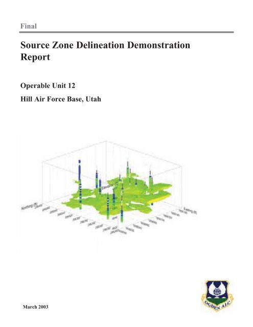
EXECUTIVE SUMMARYThis report documents the results of the Hill Air Force Base Operable Unit 12 (OU 12) Source ZoneDelineation Demonstration. The demonstration was conducted to investigate volatile organic compoundcontamination in the vadose zone of the suspected OU 12 source area using rapid decision-making basedon real-time data collected in the field via direct sampling ion trap mass spectrometry (DSITMS) for rapididentification of contaminant concentrations. The investigation consisted of two technologydemonstrations – (1) wireline cone penetrometer system for multiple tool usage and (2) soil vaporextraction (SVE) for vadose zone characterization.The Wireline CPT demonstration was conducted within the vadose zone and capillary fringe underlyingthe general area defined as the suspected source zone at OU 12. During the first four days of soilsampling using the Wireline CPT sampler, approximately 205 soil samples were collected from verticaltraces at 5 discrete locations (approximately 50 samples per day). An increase in sample collectionfrequency occurred during the last five days of field operations, where approximately 395 soil sampleswere collected from vertical traces at 11 discrete locations (approximately 80 samples per day). In total,599 soil samples were collected from vertical traces at 16 discrete locations during the nine working daysof the Wireline CPT demonstration. Samples were generally collected along 1-foot sampling intervalsfrom approximately 20 to 65 feet bgs.Inference of the magnitude and spatial extent of TCE contamination in the vadose zone at OU 12 wasaccomplished using three-dimensional modeling of TCE concentration measured in the soil samplesretrieved with the Wireline CPT sampler. An isometric view of the 100 g/kg iso-concentration surfacefrom the final three-dimensional model of TCE contamination in soil is shown in Figure ES-1. The viewis from the southwest corner of the model domain, looking to the northeast. The spheres on each of theborings represent soil sample locations, color-coded according to the measured concentration of TCE.The highest concentrations of TCE were observed in samples collected from U2-1804 at a depth of 27feet (154,000 g/kg) and 29 feet (73,000 g/kg) below ground surface (bgs); from U2-1807 at 33 feet bgs(144,000 g/kg); and from U2-1817 at 29 feet bgs (131,900 g/kg). In contrast, surrounding boringsyielded no soil samples with a measured TCE concentration greater than 10,000 g/kg. During theanalysis of samples collected from U12-1807, four samples (30 to 33 feet bgs) were observed to contain alight nonaqueous phase liquid (LNAPL). In addition, two samples (27 to 29 feet bgs) from U12-1804were observed to contain a LNAPL.Based on the results of the TCE soil model, contamination in the vadose zone at OU 12 has a distinctlylayered character. Individual layers are elliptical in plan-view, approximately 5 to 10 feet thick, severalhundreds of square feet in areal extent, and are present over most of the entire thickness of the vadosezone within the modeled region. The layers of TCE contamination tend to reside in silty-sand soils,joined vertically by narrow and tortuous throat-like connections evocative of migration pathways. Thisspatial pattern of TCE contamination in soil suggests that water, percolating downward under the force ofgravity and carrying with it dissolved TCE, spreads laterally when it encounters capillary barriers.Pathways through the barriers are ultimately found, providing the contaminated water with a new avenuefor downward percolation.March 2003 ES-1 OU 12 Demonstration ReportFinal

Figure ES-1. Iso-concentration surface of the 100 µg/kg TCE contamination in soil constructed using 599 wireline soil samplesfrom 16 borings.March 2003 ES-2 OU 12 Demonstration ReportFinal

The SVE demonstration conducted in the suspected source zone at OU 12 focused on step tests forestimating TCE distribution within the vadose zone of the investigative area using a multiphase,multicomponent numerical model. The concentration of TCE in time was monitored on one-secondintervals via the on-site laboratory using DSITMS, resulting in over 66,000 data. The TCE time-seriesdata collected during the demonstration were compared with simulated time-series data using a theoreticaldistribution of TCE mass in the zone of influence and a sequential forward numerical modeling scheme inan attempt to help delineate source-zone contamination in the vadose zone of the investigative area.Although the step tests were optimized to assess contaminant distribution within the vadose zone of theinvestigative area, the data also provide an indication of the pneumatic response of the subsurface at OU12 during vapor extraction operations. Based on a maximum radial extent of induced subsurface vacuumof 0.01 inch of water, the zone of pneumatic influence observed during the OU 12 SVE demonstrationranged from approximately 50 to 80 feet in the southern section of the investigative area to over 100 feetin the northern section. The average zone of pneumatic influence within the investigative area wasapproximately 85 feet. The average in situ air permeabilities observed during vapor extraction operationsis typical of the fine-grained material in the vadose zone at OU 12 and ranged from 5 to 20 Darcy with ageometric mean of approximately 10 Darcy.Over 160 theoretical source configurations were simulated numerically during the demonstration. Thebest correlation between the predicted and measured TCE vapor-phase concentration profile was obtainedusing a theoretical TCE source located approximately 8 feet northwest of U12-VP1 and 19 feet southeastof U12-VP2. This source was assumed to be 5 feet by 5 feet in areal extent, 10 feet thick, and containing400 mg/kg TCE. For this source configuration, the predicted vapor-phase concentrations and the generalconcentration profiles were in relatively good agreement for five of the seven extraction wells butsignificant differences were observed for two wells distant from the assumed source location. In addition,the predicted TCE concentration profiles for U12-VP1 and U12-VP2 did not exhibit the characteristicexponential decline that was observed in the measured concentrations during periods of blower shutdown.The vapor-phase concentration of TCE observed during SVE operations at OU 12 closely correlate withthe spatial distribution of the TCE soil contamination as shown in Figure ES-2. The highest TCE vaporconcentration was observed at U12-VP1 located approximately 20 feet west of the southern end of thedrum excavation area. The maximum concentration of TCE in the extracted vapor from this location wasapproximately 1,150 ppmv. The next highest concentration of TCE was observed at U12-VP2, locatedapproximately 35 feet north of U12-VP1 and 20 feet west of the north end of the drum excavation area.The maximum concentration of TCE in the extracted vapor at U12-VP2 during testing was approximately500 ppmv. The concentration of TCE in the extracted vapor from the other five wells was less thanapproximately 100 ppmv during vapor extraction operations.Although a final source configuration was not obtained with the sequential forward modeling scheme, theSVE modeling did suggest that the highest levels of soil contamination are located near the top of thescreened intervals of U12-VP1 and U12-VP2. Based on the results of the model, it is inferred that themajor source of TCE contamination is located in the upper portion of the vadose zone (20 to 35 feet bgs)offset slightly to the east of U12-VP1 and moderately more distant from U12-VP2. Based on the resultsof the SVE modeling, soil concentrations may be closely approaching the saturation limit where a denseMarch 2003 ES-3 OU 12 Demonstration ReportFinal

nonaqueous phase liquid (DNAPL) is expected to exist; however, TCE concentrations observed duringthe Wireline CPT soil investigation do not support the presence of a separate DNAPL phase. Themodeling of TCE contamination in the soil illustrated that the highest levels of soil contamination are inthe range of 100 mg/kg to 200 mg/kg and are located near the top of the screened intervals of U12-VP1and U12-VP2. Thus, it is likely that the major TCE contamination in the investigative area is associatedwith a sorbed fraction and probably a separate LNAPL phase that was identified in the vicinity of vaporextraction wells U12-VP1 and U12-VP2 during the Wireline CPT soil investigation (soil samples thatexhibited LNAPL also were shown to contain elevated concentrations of TCE).March 2003 ES-5 OU 12 Demonstration ReportFinal

TABLE OF CONTENTSEXECUTIVE SUMMARY ................................................................................................................. ES-11.0 INTRODUCTION ....................................................................................................................1-11.1 Project Objectives............................................................................................................1-11.2 Dynamic Work Plan Approach........................................................................................1-11.3 Overview of Source Zone Delineation Tasks..................................................................1-51.4 Report Organization.........................................................................................................1-62.0 SITE DESCRIPTION ...................................................................................................................2-12.1 Site Description ...............................................................................................................2-12.2 Suspected Contaminant Source .......................................................................................2-12.3 Preliminary Vadose Zone Stratigraphy ...........................................................................2-33.0 WIRELINE CPT SOIL SAMPLING DEMONSTRATION.........................................................3-13.1 Wireline CPT Technical Approach .................................................................................3-13.2 Wireline CPT Implementation and Operations ...............................................................3-33.3 DSITMS Soil Analytics...................................................................................................3-64.0 SOIL VAPOR EXTRATION DEMONSTRATION....................................................................4-14.1 SVE Technical Approach ................................................................................................4-14.2 SVE Implementation and Operations ..............................................................................4-44.3 DSITMS Vapor Analytics .............................................................................................4-125.0 RESULTS OF SOIL SAMPLING AND SVE DEMONSTRATION ..........................................5-15.1 OU 12 Soil Data Evaluation ............................................................................................5-15.1.1 Magnitude and Spatial Extent of TCE Contamination in Soil ...........................5-65.1.2 Soil Architecture of the Vadoze Zone ..............................................................5-135.1.2.1 Site-Wide Soil Architecture Model .....................................................5-195.1.2.2 Combined Modeling of Soil Architecture and TCE Contamination ...5-275.2 OU 12 SVE Evaluation..................................................................................................5-315.2.1 Pneumatic Evaluation .......................................................................................5-315.2.1.1 Zone of Pneumatic Influence...............................................................5-315.2.1.2 In Situ Permeability .............................................................................5-345.2.1.3 Blower Comparison.............................................................................5-425.2.2 TCE Vapor Concentrations ..............................................................................5-435.2.3 Vapor Transport Modeling...............................................................................5-565.2.3.1 Vacuum Distribution ...........................................................................5-575.2.3.2 Sequential Forward Modeling .............................................................5-596.0 COST ANALYSIS .......................................................................................................................6-16.1 Conventional Sampling and Analysis..............................................................................6-26.1.1 Hollow Stem Auger (HSA).................................................................................6-56.1.2 Direct Push technology (DPT) ...........................................................................6-6Pageii

6.2 Adaptive Sampling and Analysis.....................................................................................6-66.2.1 Wireline Sampler/DSITMS (WS/DSITMS).......................................................6-66.2.2 Soil Vapor Extraction/DSITMS (SVE/DSITMS) ............................................6-106.3 Summary........................................................................................................................6-117.0 CONCLUSIONS AND RECOMMENDATIONS........................................................................7-17.1 Demonstration Results.....................................................................................................7-17.1.1 Wireline CPT Soil Sampling ..............................................................................7-17.1.2 SVE for Characterization....................................................................................7-27.1.3 DSITMS Field Analytics ....................................................................................7-37.2 OU 12 Vadose Zone Contaminant Distribution ..............................................................7-37.3 Recommendations............................................................................................................7-78.0 REFERENCES ...........................................................................................................................8-1APPENDIX AAPPENDIX BField Analytical Results for the Wireline Soil DemonstrationSimulated TCE Vapor-Phase Concentration Profiles for OU 12 SVEDemonstrationiii

LIST OF FIGURESFigure ES-1 Iso-Concentration surface of the 100 g/kg TCE contamination in soilconstructed using 599 Wireline soil samples from 16 borings..................................... ES-2Figure ES-2 TCE vapor phase and soil concentrations..................................................................... ES-4Figure 1-1 Location map ...................................................................................................................1-2Figure 1-2 OU 12 source zone demonstration Core Technical Team...............................................1-4Figure 2-1 OU 12 site map showing TCE plume ..............................................................................2-2Figure 2-2 Recently discovered drums located near ground surface at OU 12.................................2-3Figure 2-3 Simplified representation of vadose zone stratigraphy ...................................................2-4Figure 3-1 Initial proposed Wireline CPT sampling transects..........................................................3-2Figure 3-2 Wireline locking and retrieval mechanism......................................................................3-4Figure 3-3 Illustration of the OU 12 Wireline CPT soil sampling demonstration............................3-5Figure 4-1 Schematic of VENT3D structure.....................................................................................4-2Figure 4-2 Predicted TCE distribution in vapor-phase following 30 years of diffusivetransport in a homogeneous permeability field of 1 darcy ..............................................4-4Figure 4-3 Predicted concentration of TCE in extracted soil vapor..................................................4-5Figure 4-4 Typical extraction/monitoring well .................................................................................4-6Figure 4-5 Soil vapor extraction system process & instrumentation diagram ..................................4-8Figure 4-6 Field-portable SVE process system and extraction/monitoring well completions..........4-9Figure 4-7 Results of regression analysis performed on the OU 12 SVE calibration data.............4-13Figure 5-1 Location and extent of modeling domains and SVE and Wireline sampler boringlocations...........................................................................................................................5-2Figure 5-2 TCE concentration depth profiles less than 350 g/kg for the OU 12 WirelineCPT soil sampling demonstration....................................................................................5-3Figure 5-3 TCE concentration depth profiles less than 1000 g/kg for the OU 12 WirelineCPT soil sampling demonstration....................................................................................5-5Figure 5-4 Soil samples collected from U12-1807 (30 to 33 feet bgs) containing LNAPL .............5-7Figure 5-5 Initial model of TCE contamination in soil, 100 g/kg iso-concentration surface,constructed using 294 Wireline soil samples from seven borings...................................5-9Figure 5-6 Initial model of TCE contamination in soil, 1000 g/kg iso-concentration surface,constructed using 294 Wireline soil samples from seven borings.................................5-10Figure 5-7 Revised model of TCE contamination in soil, 100 g/kg iso-concentration surface,constructed using 419 Wireline soil samples from 10 borings......................................5-11Figure 5-8 Revised model of TCE contamination in soil, 1000 g/kg iso-concentration surface,constructed using 419 Wireline oil samples from 10 borings .......................................5-12Figure 5-9 Final model of TCE contamination in soil, 100 g/kg iso-concentration surface,constructed using 599 Wireline soil samples from 16 borings......................................5-14Figure 5-10 Final model of TCE contamination in soil, 1000 g/kg iso-concentration surface,constructed using 599 Wireline soil samples from 16 borings......................................5-15iv

Figure 5-11 Final model of TCE contamination in soil, 10,000 g/kg iso-concentration surface,constructed using 599 Wireline soil samples from 16 borings......................................5-16Figure 5-12 Isometric view, lookng northeast of the final model of TCE contamination in soil,100 g/kg iso-concentration surface, constructed using 599 Wireline soil samplesfrom 16 boring ...............................................................................................................5-17Figure 5-13 Isometric view, looking northeast, of the soil-type data used to model the sitewidevadose zone soil architechture at OU 12 ..............................................................5-20Figure 5-14 Isometric view, looking northeast, of a block diagram of the site-wide vadosezone soil architecture model ..........................................................................................5-21Figure 5-15 East-west vertical cross-section through the site-wide soil architecture model ata northing of 298,000 ft. ................................................................................................5-23Figure 5-16 East-west vertical cross-section through the site-wide soil architecture model ata northing of 298,200 ft. ................................................................................................5-24Figure 5-17 East-west vertical cross-section through the site-wide soil architecture model ata northing of 298,600 ft.. ...............................................................................................5-25Figure 5-18 North-south vertical cross-section through the site-wide soil architecture modelat an easting of 1,856,150 ft. .........................................................................................5-26Figure 5-19 East-west vertical cross-section through the combined TCE/soil model at anorthing of 298,270 ft....................................................................................................5-28Figure 5-20 North-south vertical cross-section through the combined TCE/soil model at aneasting of 1,856,110 ft. ..................................................................................................5-30Figure 5-21 Idealized streamlines and vacuum distribution during SVE operations........................5-32Figure 5-22 Vacuum distribution as a function of distance measured during the OU 12 SVEdemonstration ................................................................................................................5-33Figure 5-23 Pressure decrease as a function of time during vapor extraction at U12-VP1 ..............5-36Figure 5-24 Pressure decrease as a function of time during vapor extraction at U12-VP2 ..............5-37Figure 5-25 Pressure decrease as a function of time during vapor extraction at U12-VP3 ..............5-38Figure 5-26 Pressure decrease as a function of time during vapor extraction at U12-VP5 ..............5-39Figure 5-27 Pressure decrease as a function of time during vapor extraction at U12-VP7 ..............5-40Figure 5-28 Predicted steady-state flow rates as a function of soil permeability for variousapplied vacuum Pw........................................................................................................5-41Figure 5-29 Induced airflow at U12-VP1 as a function of applied vacuum for both blowers..........5-43Figure 5-30 TCE vapor data obtained at U12-VP1 during OU 12 SVE demonstration ...................5-45Figure 5-31 TCE vapor data obtained at U12-VP2 during OU 12 SVE demonstration ...................5-46Figure 5-32 TCE vapor data obtained at U12-VP3 during OU 12 SVE demonstration ...................5-47Figure 5-33 TCE vapor data obtained at U12-VP4 during OU 12 SVE demonstration ...................5-48Figure 5-34 TCE vapor data obtained at U12-VP5 during OU 12 SVE demonstration ...................5-49Figure 5-35 TCE vapor data obtained at U12-VP6 during OU 12 SVE demonstration ...................5-50Figure 5-36 TCE vapor data obtained at U12-VP7 during OU 12 SVE demonstration ...................5-51Figure 5-37 Screened intervals of the vapor extraction wells in relation to the modeledvadose zone soil architecture.........................................................................................5-53v

Figure 5-38 Horizontal slices at five-foot increments through the soil architecture showingscreened Intervals of vapor extraction wells .................................................................5-54Figure 5-39 Vacuum distribution predicted at 40 to 45 feet bgs during vapor extraction fromU12-VP2 for 6 Hours at 12 scfm assuming a two-layer permeability field ..................5-58Figure 5-40a Spatial locations of simulated source areas...................................................................5-63Figure 5-40b Spatial locations of simulated source areas...................................................................5-64Figure 5-40c Spatial locations of simulated source areas...................................................................5-65Figure 5-40d Spatial locations of simulated source areas...................................................................5-66Figure 5-40e Spatial locations of simulated source areas...................................................................5-67Figure 5-41 Predicted versus measured TCE concentrations at U12-VP1 and U12-VP2 forsource area #1 ................................................................................................................5-68Figure 5-42 Predicted versus measured TCE concentrations at U12-VP1 and U12-VP2 forsource area #2 ................................................................................................................5-70Figure 5-43 Predicted versus measured TCE concentrations at U12-VP1 for source area #6..........5-71Figure 5-44 Predicted versus measured TCE concentrations at U12-VP1, U12-VP2, U12-VP3,U12-VP4, and U12-VP6 for source area #7 ..................................................................5-72Figure 5-45 TCE soil concentration (mg/kg) at 25 to 30 feet bgs after diffusion period andprior to vapor extraction operations (source area 7)......................................................5-73Figure 5-46 TCE soil concentration (mg/kg) at 25 to 30 feet bgs prior to and after Soil Vaporextraction operation at U12-VP2...................................................................................5-74Figure 5-47 TCE soil gas concentration (ppmv) prior to and following soil vapor extractionfrom U12-VP2 ...............................................................................................................5-75Figure 5-48 Predicted versus measured TCE concentrations at U12-VP1 for source area #9..........5-77Figure 5-49 Predicted versus measured TCE concentrations at vapor extraction wells for400 mg/kg TCE in source area #9 .................................................................................5-78Figure 5-50 Contours of TCE soil concentrations (mg/kg) for source area 10 using the EVSaverage layer model.......................................................................................................5-80Figure 5-51 Contours of TCE soil concentrations (mg/kg) for source area 10 using the EVSmaximum layer model ...................................................................................................5-81Figure 5-52 Predicted versus measured TCE concentrations at vapor extraction wells for EVSaverage soil concentrations in source area #10 .............................................................5-82Figure 5-53 Predicted versus measured TCE concentrations at vapor extraction wells for EVSmaximum soil concentrations in source area #10..........................................................5-83Figure 5-54Figure 7-1Permeability effects on the predicted TCE vapor-phase concentration profile.............5-85Iso-concentration surface of the 100 g/kg TCE contamination in soilconstructed using 599 Wireline soil samples from 16 borings........................................7-4Figure 7-2 TCE vapor phase and soil concentrations........................................................................7-6Figure 7-3 NAPL dilution factor as a function of TCE sample concentration .................................7-7vi

LIST OF TABLESTable 3-1 Summary of Wireline CPT QA Sample Analyses...........................................................3-7Table 4-1 Soil Vapor Extraction/Monitoring Well Specifications ..................................................4-5Table 4-2 Instrumentation Utilized During the OU 12 SVE Demonstration.................................4-10Table 4-3 Summary of SVE Step Tests .........................................................................................4-11Table 5-1 Summary of Wireline CPT Soil Sampling Program........................................................5-6Table 5-2 Modeling Domain for TCE Contamination and Combined Soil/TCE Modeling............5-7Table 5-3 Modeling Domain for Site-Wide Soil Model ................................................................5-18Table 5-4 Distribution of TCE Greater Than 10 g/kg by Soil Type............................................5-29Table 5-5 Estimated In Situ Air Permeability................................................................................5-41Table 5-6 Percentage of Soil Type in Screened Interval of Vapor Extraction Wells....................5-52Table 5-7 Comparison of Measured and Predicted Vacuum Distribution.....................................5-59Table 5-8 OU 12 SVE Sequential Forward Modeling Scenarios ..................................................5-60vii

LIST OF ACRONYMS AND ABBREVIATIONSAFBAir Force BaseARAApplied Research Associates, Inc.amslAbove Mean Sea LevelbgsBelow Ground Surfacecis-1,2-DCE cis-1,2-DichloroethenecfmCubic Feet per MinuteCPTCore Penetrometer TestCSMConceptual Site ModelDCEDichloroetheneDNAPLDense Nonaqueous Phase LiquidDSITMSDirect Sampling Ion Trap Mass SpectrometryEPAEnvironmental Protection AgencyEPRIMSEnvironmental Resources Program Management SystemHgMercuryHPHorse PowerLNAPLLight Nonaqueous Phase LiquidMAMS-2Missile Assembly Maintenance and Storage-2mbarMillibarMeOHMethanolMWHMontgomery Watson HarzaNANot ApplicableNAPLNonaqueous Phase LiquidOU 12 Operable Unit 12PCETetrachloroethanePECPerformance Evaluation CheckppbPart-per-BillionppmvPart-per-Million by VolumePVCPolyvinyl ChorideQAQuality AssuranceQA/QCQuality Assurance/Quality ControlROIRadius of InfluencescfmStandard Cubic Feet per MinuteSTPStandard Temperature and PressureSVESoil Vapor ExtractionTCETrichloroetheneTVDTotal Variation DiminishingVOCVolatile Organic Compoundviii

1.0 INTRODUCTIONThis report documents the results of the Source Zone Delineation Demonstration at Operable Unit 12 (OU12), Hill Air Force Base (AFB) in Utah (see Figure 1-1). The demonstration was conducted to investigatevolatile organic compound (VOC) contamination in the vadose zone of the suspected OU 12 source areausing rapid decision-making based on real-time data collected in the field via a dynamic work planapproach. The investigation consisted of two technology demonstrations – (1) wireline cone penetrometersystem for multiple tool usage and (2) soil vapor extraction (SVE) for vadose zone characterization.Sampling and analysis was conducted in the field via direct sampling ion trap mass spectrometry(DSITMS) for rapid identification of contaminant concentrations. Real-time data was required due to therapid soil sampling capability of the wireline tool and to obtain adequate characterization of vapor-phasecontaminant concentration profiles as a function of time across a varied flow regime. Additionally,optimization of vapor extraction rates and location of investigation was optimized as a result ofimmediate concentration profiles. This investigation represents the next progression in thecharacterization of OU 12 and builds upon the active soil-gas survey completed in the suspected sourcezone at OU 12 in October 2001 and March 2002 [MWH, 2002a].1.1 Project ObjectivesThe objectives for the Source Zone Delineation Demonstration at OU 12 included:Locating and spatially-defining any existing source of trichloroethene (TCE) in the vadose zone andcapillary fringe of the suspected OU 12 source zone;Demonstrating the ability of ARA’s Wireline CPT system and Tri-Corders Environmental, Inc.DSIMTS to rapidly characterize contaminant distribution within the vadose zone; andDemonstrating the ability of SVE to characterize the spatial and phase distribution of VOC masswithin the vadose zone.1.2 Dynamic Work Plan ApproachA dynamic work plan approach was utilized during the OU 12 Source Zone Delineation Demonstration.The dynamic work plan approach focuses on the decision-making process that integrates the datagenerated in the field to facilitate a rapid, cost effective characterization of the site. Formulated as adecision tree during the planning process, the dynamic work plan adapts site investigative activities inrelation to the evolving, usually on a daily basis, conceptual site model (CSM). Dynamic work planshave been successfully demonstrated for over ten years by various parties [Burton, 1993 and Robbat,1997]. Implementation of a dynamic work plan requires on-site generation and interpretation of data sothat results are available fast enough to support the rapidly evolving on-site decision-making. Althoughnot a new concept, recent advances in field analytical instrumentation and computerization have enableddynamic work plans to be utilized in the characterization of complex sites.March 2003 1-1 OU 12 Demonstration ReportFinal

Hill Air Force BaseUtahRIVERDALEWeber River8015SALT LAKE CITY70ROYOperable Unit 12(OU 12)RoyGateNorthGateWeber CountyDavis CountySUNSETCLINTONHILLAIR FORCEBASEWestGateDavis - Weber CanalCLEARFIELDSouthWestGateSouthGateLAYTONLocation MapOperable Unit 12 (OU 12)Hill Air Force Base, Utah0.4 0 0.4 0.8MilesFIGURE 1-1March 2003 1-2 OU 12 Demonstration ReportFinal

Dynamic work plans rely on an adaptive sampling and analysis strategy. Rather than specify thesampling location and frequency, dynamic work plans specify the decision-making logic that will be usedin the field to determine where to collect samples and when to terminate sampling. The conceptual modelof the site is dynamic and changes to reflect the increased site knowledge gained from site investigativeactivities. Thus, an adaptive sampling program changes as the CSM is refined based on the analyticalresults produced in the field. In comparison, the traditional site investigation work plan is static in natureand depends on pre-specified sampling locations, sampling frequency, and the types of analysis to beperformed.A dynamic work plan approach requires detailed up-front planning, an advanced level of field-basedtechnology and interpretative expertise, and the flexibility to make assessment decisions during fieldoperations. Real-time, or near real-time visualization and interpretation of field-generated data enables adynamic decision process to direct data collection during the site investigation activities. This approachemploys multiple measurement and sampling technologies coupled with on-site technical decisionmakingby a skilled, multidisciplinary Core Technical Team. The purpose of the Core Technical Team isto provide a continuous, integrated, multidisciplinary presence throughout the project. Additionally, theCore Technical Team is responsible for decision-making in the field and directing the site investigation.The technical team generally is composed of professionals that possess expertise in geology,hydrogeology, analytical chemistry, and chemical/remediation process systems. The Core TechnicalTeam for the OU 12 Source Zone Delineation Demonstration consisted of members from URSCorporation, Applied Research Associates, Inc. (ARA), Tri-Corders Environmental, Inc., MontgomeryWatson Harza (MWH), and Hill AFB (see Figure 1-2).As the prime contractor, URS was responsible for the design, implementation, and reporting requirementsassociated with the Source Zone Delineation Demonstration. Additionally, URS conducted the SVEinvestigation at OU 12 to serve as a technology demonstration for the utility of SVE as a characterizationtool for VOC contamination in the vadose zone. To aid in the characterization of the OU 12 source zoneand provide preliminary site data for the placement of the soil vapor monitoring probes, ARA conducted aWireline CPT investigation. The Wireline CPT investigation also served as a technology demonstrationfor the rapid characterization of a VOC source zone. The Wireline CPT system consists of an innovativeretrieval system and an assortment of characterization tools that can be retrieved and interchanged fromany depth in the vadose zone without retracing the rod-string from the ground. Tri-CordersEnvironmental, Inc. provided field analytical services for the rapid analysis of low concentration VOCs inthe environmental media analyzed at OU 12. Field analysis included the use of DSITMS for nearcontinuous analysis of soil and vapor samples collected via the Wireline CPT and soil vapor extractionsystems. MWH assisted with the installation of the vapor extraction/monitoring probes and with datalogging during the Wireline CPT demonstration.Members of the team were responsible to make recommendations on field investigative activities (e.g.,sampling locations and frequency) based on the preliminary CSM of the site and the most current datagathered during field operations. Although the URS Project Manager and ARA Project Manager servedas team co-leaders, final decision-making authority resided with the URS Project Manager during thedemonstration.March 2003 1-3 OU 12 Demonstration ReportFinal

Co-Team LeaderCo-Team LeaderURS Project ManagerURS Project ManagerCharles Holbert, Ph.D.Charles Holbert, Ph.D.(Chemical Engineer)(Chemical Engineer)Co-Team LeaderCo-Team LeaderARA Project ManagerARA Project ManagerJoel Hayworth, Ph.D.Joel Hayworth, Ph.D.(Environmental Engineer)(Environmental Engineer)Team MemberTeam MemberTri-Corders Environmental, Inc.Tri-Corders Environmental, Inc.Bill Davis, Ph.DBill Davis, Ph.D(Analytical Chemist)(Analytical Chemist)Team MemberTeam MemberMWHMWHHhan OlsenHhan Olsen(Hydrogeologist)(Hydrogeologist)Team MemberTeam MemberHill Air Force BaseHill Air Force BaseKyle GorderKyle Gorder(Environmental Engineer)(Environmental Engineer)Figure 1-2. OU 12 source zone demonstration Core Technical Team.March 2003 1-4 OU 12 Demonstration ReportFinal

1.3 Overview of Source Zone Delineation TasksThe delineation of the suspected source zone at OU 12 was conducted using a dynamic work planapproach. To ensure the project objectives were met, field operations were performed according to thefollowing strategy:Up-front systematic planning;Use of an adaptive (dynamic) sampling plan;On-site analysis and “immediate” availability of results using the DSITMS; andRapid on-site decision-making by the Core Technical Team and guided by real-time data.The primary tasks associated with the Source Zone Delineation Demonstration included the following:Task 1. Mobilization and Setup. The CPT truck was mobilized to the OU 12 site and the wirelinesampling tool system was prepared for field operations. The on-site laboratory consisting of the DSITMSalso was mobilized to the OU 12 site and initialized for field operations.Task 2. Wireline CPT Demonstration. The Wireline CPT investigation was conducted within thevadose zone and capillary fringe underlying the suspected source zone at OU 12. The investigationfocused on TCE analysis of vadose zone soils, since the TCE groundwater plume emanating from OU 12had been previously defined. Soil sampling began along a pre-determined sampling transect and one-footvertical intervals from the ground surface. Characterization of the spatial extent and magnitude of TCEcontamination in the vadose zone was concurrent with field sampling efforts. Iterative, short-delaymodeling of the extent of contamination provided field personnel with guidance for selecting newWireline CPT sampling locations.Task 3. Vapor Extraction/Monitoring Probe Installation. Soil vapor monitoring/extraction probes wereinstalled at seven locations in the suspected OU 12 source zone using direct push technology. At eachlocation, probes were installed from approximately 30 to 60 feet below ground surface (bgs) withscreened intervals ranging from 15 to 20 feet in length. Exact depths and locations were based uponreview of the Wireline CPT data collected during the project.Task 4. SVE Demonstration. The SVE system was constructed and operated for approximately 5 daysin the suspected source zone at the OU 12 site. The SVE system was operated at varied rates of flow todetermine vapor phase contaminant concentration profiles under both advective and diffusive dominatedflow regimes.March 2003 1-5 OU 12 Demonstration ReportFinal

1.4 Report OrganizationThe remaining sections of this report are organized as follows:Section 2.0 provides a summary of the OU 12 site, including a description of the suspectedcontaminant source and the vadose zone stratigraphy.Section 3.0 summarizes the Wireline CPT technical approach, field implementation, and DSITMSsoil analytics.Section 4.0 summarizes the SVE technical approach, field implementation, and DSITMS vaporanalytics.Section 5.0 presents the results of the Wireline CPT soil sampling and SVE demonstration.Section 6.0 provides a cost comparison between conventional vadose zone investigationmethodologies and the technologies demonstrated as part of this project.Section 7.0 presents conclusions and recommendations based on the results of the demonstration.March 2003 1-6 OU 12 Demonstration ReportFinal

2.0 SITE DESCRIPTIONThis section provides a summary of the OU 12 site. Several environmental investigations have beenconducted at the OU 12 site (formerly part of OU 5), including CPT investigations, aquifer testing,groundwater and soil sampling, hydraulic flow and contaminant transport modeling, and two active soilgassurveys.2.1 Site DescriptionThe OU 12 site is located in the northwestern region of Hill AFB, near the western boundary of the Base(see Figure 1-1). Environmental investigations at OU 5 in 2000 identified contamination beneath the Cityof Roy. This plume (above the maximum contaminant level [MCL] of 5 g/L) and the on-Basecontamination were designated as OU 12 in October 2001 [MWH, 2002b]. The primary contaminant ofconcern in the groundwater at OU 12 is TCE. Other contaminants of concern at OU 12 include cis-1,2-dichloroethene (cis-1,2-DCE), carbon tetrachloride, and tetrachloroethene (PCE).The on-Base portion of OU 12 is located just inside of the Base perimeter fence and west of the MissileAssembly Maintenance and Storage-2 (MAMS-2) area. The area of activity consists of relatively flat,unpaved open space dominated by sagebrush and rabbit brush. Remnants of a former WastewaterTreatment Plant are located in the southeastern part of the site. Debris is scattered across the site,including several rusted-through half-buried drums, abandoned foundations, and various small metallicobjects. Several trench-like features also are present in the area.2.2 Suspected Contaminant SourceAlthough the source of the TCE groundwater plume at OU 12 had not been identified, a soil-gas surveyindicated the suspected source area is northwest of the former Wastewater Treatment Plant. Additionally,increasing and/or highly variable TCE concentrations in monitoring well U9-16-011 indicated acontinuing source in the area north of the former Wastewater Treatment Plant [MWH, 2002a]. A welldelineatedTCE groundwater plume emanates from the suspected source zone at OU 12 as shown inFigure 2-1. The local groundwater flow direction is to the west, towards the town of Roy, Utah and theGreat Salt Lake. The TCE groundwater plume extends down gradient approximately 8,000 feet;variations in plume width from origin to terminal end-point are small (average width of approximately500 feet). From plume origin terminus, depth to the plume varies from approximately 85 feet bgs (at theorigin) to approximately 4 feet bgs in the area of monitoring well U5-1143 off Base. Concentrations ofTCE as high as 1,300 g/L have been detected off Base at monitoring well U5-1112 [MWH, 2002a].Within the suspected source zone, depth to groundwater is approximately 70 feet bgs.Prior to this project, attempts to locate and delineate the spatial distribution of the suspected TCE sourcezone have been minimal (with the exception of the recent soil-gas survey). However, indirect evidencestrongly supported the possible presence of a TCE source zone within the vadose zone (primarily) andthe capillary fringe (secondarily) underlying the OU 12 site. This indirect evidence suggests that TCE isMarch 2003 2-1 OU 12 Demonstration ReportFinal

Davis-Weber CanalDetail AreaHillAir ForceBaseROYOperable Unit 12 (OU 12)TCE PlumeRoyGateWeber CountyDavis CountyCLINTONSource Investigation AreaTCE Concentrations ( g/L)5 - 1010 - 100100 - 10001000 - 10000SUNSETHILLAIR FORCEBASEAdapted from:Montgomery Watson Harza , 2002.Draft Operable Units 5 and 12Active Soil-Gas Survey Source AreaInvestigation ReportHill Air Force Base, Utah, April 2002.Site map showing TCE PlumeOperable Unit 12 (OU 12)Hill Air Force Base, Utah500 0 500 1,000FeetFIGURE 2-1March 2003 2-2 OU 12 Demonstration ReportFinal

held as a residual phase within the unsaturated soils and possibly within a capillary smear zone underlyingOU 12. Indirect evidence supporting the presence of a vadose zone TCE source area included:A well-defined groundwater plume with high TCE groundwater concentrations in the central, nearsourceregion (see Figure 2-1).Results of recent soil gas surveys defining the presence of TCE in soil gas within the vadose zoneunderlying OU 12. The recent discovery of buried drums near the ground surface generally correlated with soil-gassurvey results (see Figure 2-2). The presence of a solid ash-like material within a drum having TCE concentrations exceeding 16,000mg/kg.The apparent absence of pure-phase TCE within the saturated zone underlying OU 12 (as indicated bypast investigations).Fluctuations in groundwater TCE concentrations in down-gradient monitoring wells suggestingperiodic dissolution of residual-phase TCE within the vadose zone during infiltration events, and/orperiodic dissolution of TCE within the capillary smear zone during changes in the local water tableelevation.2.3 Preliminary Vadose Zone StratigraphyThe vadose zone stratigraphy of the OU 12 site is complex. The upper portion consists mainly of sandwith gravel and silty-sand interbeds, grading to increasing amounts of sandy-silt and silt with depth. Thehighest measured concentrations of TCE in the soil gas appear to be associated with the deeper, finergrainedintervals. Depth to groundwater increases from approximately 50 feet bgs in the south to 80 feetbgs in the north. The cross-section shown in Figure 2-3 illustrates the initial conceptualization of thevadose zone stratigraphy, based on a generalized interpretation of logs from CPT borings advancedduring a soil gas survey conducted at the site in late 2001 and early 2002 [MWH, 2002a].Figure 2-2. Recently discovered drums located near ground surface at OU 12.March 2003 2-3 OU 12 Demonstration ReportFinal

ANorthSouthU5-18864,580CROSS SECTION A - A' LOOKING EASTOperable Unit 12A'U5-1867U5-1912U5-1913U5-1895U5-1874U5-1875U5-1885U5-1890U5-1919U5-1891U5-1917U5-1903U5-1898U5-1907U5-18974,5604,5404,5204,500TD 81.2'TD 84.48'TD 75.14'TD 70.05' TD 70.54' TD 70.05'TD 60.54'TD 70.05'TD 72.01'Extent of Underlying Trichloroethene (TCE) Groundwater PlumeTD 70.05'TD 71.03'TD 65.13'TD 66.11'TD 57.31'Former Wastewater Treatment PlantTD 65.13'5-10 g/L 10-100 g/L 5-10 g/LTD 133.37'AHILLAIR FORCEBASEDavis-Weber CanalHill Air Force Base BoundaryElevation (ft amsl)2010040 80Vertical Scale in FeetHorizontal Scale in FeetAdapted from:Montgomery Watson Harza , 2002. Draft Operable Units 5 and 12Active Soil-Gas Survey Source Area Investigation ReportHill Air Force Base, Utah, April 2002.U5-1890OU 12 TCE PlumeLithologyA'FormerWastewaterTreatmentPlantSandSand With Interbedded SiltSilt With Interbedded SandSiltSoil-Gas Sampling LocationApproximate Location ofGroundwater TableSimplified Representation ofVadose Zone Stratigraphy2nd Street0 500FeetOperable Unit 12 (OU 12)Hill Air Force Base, UtahCross Section Location MapFIGURE 2-3March 2003 2-4 OU 12 Demonstration ReportFinal

3.0 WIRELINE CPT SOIL SAMPLING DEMONSTRATIONThe design of the Wireline CPT demonstration was based on data obtained from previous siteinvestigation and characterization activities conducted at OU 12. To formulate the design basis,numerous data sources were reviewed, including site stratigraphy obtained from cone penetrometersoundings, groundwater analytical data, and soil-gas concentration data obtained during the two phases ofsoil-gas sampling conducted within the suspected OU 12 source zone. These data were used to formulatethe preliminary CSM and identify the initial sampling plan associated with the Wireline CPTinvestigation. An adaptive sampling and analysis strategy was used during the demonstration and wasbased on field-generated data subjected to professional interpretation by the Core Technical Team.Characterization of the spatial extent and magnitude of TCE contamination in the vadose zone wasconcurrent with field sampling efforts. Iterative, short-delay modeling of the extent of contaminationprovided field personnel with guidance for selecting new Wireline CPT sampling locations during siteinvestigation activities.3.1 Wireline CPT Technical ApproachThe Wireline CPT demonstration was conducted within the vadose zone and capillary fringe underlyingthe general area defined as the suspected zone at OU 12. The investigation focused on TCE analysis ofvadose zone soils, since the TCE groundwater plume emanating from OU 12 had been previouslydefined.Based on the indirect evidence cited in Section 2.0 of this report in relation to the suspected source zonelocation, high-density soil sampling and analysis coupled with a judgment-based decision process forsample selection was utilized during the Wireline CPT demonstration. Judgment-based samplingdecisions were intended to maximize the likelihood of locating and delineating the suspected TCE sourcezone at OU 12 within the limited deployment time allocated. The total decision error (sampling error andmeasurement error) associated with this demonstration was minimized by the following:Collecting a high number of soil samples within a vertical trace using CPT coupled with the Wirelinesoil sampler.Processing a high number of soil samples using Tri-Corders Environmental, Inc.'s DSITMS (EPASW 846 modified method 5035).Providing a high number of quality assurance (QA) samples relative to the number of site samplesusing the DSITMS.Using a judgment-based sampling and analysis strategy based on in-field expertise to guide soilsampling and analysis.The initial proposed sampling transect for the Wireline CPT demonstration is shown in Figure 3-1. Thisinitial sampling transect was based on the fact that the recently discovered buried drums did not correlateexactly with the apparent origin of the groundwater plume or the highest concentration of TCE observedduring the soil-gas survey at OU 12. It was surmised that any TCE trapped within the vadose zone wasMarch 2003 3-1 OU 12 Demonstration ReportFinal

Approx. LocationOf BarrelsInitial SamplingTransectSecondary SamplingTransectsFigure 3-1. Initial proposed Wireline CPT sampling transects.March 2003 3-2 OU 12 Demonstration ReportFinal

likely present between the drum discovery area and the origin of the groundwater plume. As illustrated inFigure 3-1, initial sampling was proposed along a straight line roughly connecting the barrel location withthe plume origin. However, an adaptive sampling and analysis strategy was used during thedemonstration and was based on field-generated data subjected to professional interpretation by the CoreTechnical Team. Characterization of the spatial extent and magnitude of TCE contamination in thevadose zone was concurrent with field sampling efforts. Iterative, short-delay modeling of the extent ofcontamination provided field personnel with guidance for selecting new Wireline CPT sampling locationsduring site investigation activities. Other potential sampling transects which were considered during theWireline CPT demonstration also are shown in Figure 3-1. These potential transects form concentriccircles expanding outward from the barrel location to the western property boundary.3.2 Wireline CPT Implementation and OperationsThe Wireline CPT system is an advancement of conventional CPT that allows nearly all characterizationwork to be accomplished in a single penetration. The Wireline CPT system, unlike conventional CPT, iscapable of retrieving and interchanging CPT “tools” without retracting the rod-string from the ground.Retracting and repenetrating the rod-string is a time consuming process because the rod string is made upof one-meter sections connected by threaded couplings. Retraction and repenetration involvesdissasembly and reassembly of the entire rod-string.The Wireline system utilizes slightly larger rods than conventional CPT (two inches in diametercompared to the 1.75-inch diameter of a standard CPT rod), allowing passage of tools through the rod’shollow center. The Wireline system also has a unique locking/release mechanism that allows interchangeof tools by a retrieval wire. The locking mechanism is identical for each individual Wireline tool, toallow interchangeability. The lock mechanism utilizes two horizontally opposed, horizontally rotatinglocking "dogs" which, when engaged, occupy a slot formed in the interior of a rod segment. Whenupward force is applied to the locking wedge via tension on a retrieval wire, the wedge slides upwardallowing the dogs to move freely inward. The dogs retract into the lock housing which allows the tool tobe retrieved to ground surface. The locking wedge is spring loaded, so outward pressure is applied to thedogs. An illustration of the locking and retrieval mechanism with the soil sampler in place is provided inFigure 3-1.With conventional CPT, multiple tools can be deployed in a single penetration by stacking multiple toolsin series on the same rod-string. This method is effective, but the number and type of tools that can bedeployed together is limited. This method is not effective for collecting multiple soil samples. TheWireline soil sampler is especially effective when collecting multiple-depth soil samples. Using theWireline system, core samples can be collected from multiple depths without retracting the rod-string.Using conventional CPT, the entire rod-string would have to be retracted to retrieve each soil sample andre-penetrated to collect another sample.March 2003 3-3 OU 12 Demonstration ReportFinal

Figure 3-2. Wireline locking and retrieval mechanism.Soil samples were collected using the CPT coupled with the Wireline soil sampler. Samples for fieldbasedanalysis using DSITMS were removed from the bottom of the Wireline soil sampler core barrelsusing a syringe sampler (approximately 10 grams of sample), placed directly into tared 40 ml VOA vials,weighed, and delivered to the DSITMS for analysis (see Figure 3-2). The 40 ml VOA vials containedapproximately 20 ml of distilled water or 10 ml of methanol as an extractant. Following submittal to theon-site laboratory, the vials were filled with additional extractant, re-weighed, and analyzed using EPAMethod 5035. The final weights of extractant and soil were used to calculate contaminant concentrationsin each sample collected.Mobilization and process system setup for the Wireline CPT soil sample collection system and DSITMSon-site laboratory began on 19 August 2002. Full soil sampling operations began on 21 August 2002following two days of system setup and troubleshooting. Several operational problems occurred duringthe first 4 days (21 – 24 August 2002) of soil sampling using the Wireline CPT sampler. Poor samplerecovery resulted in the accumulation of dirt/grit in the locking and retrieval mechanism of the wirelinetool. Subsequently, a significant amount of time was spent trying to lock and unlock the wireline tool,and on several occasions the Wireline CPT rod had to be retracted in order to clean the interior of thelocking dogs. During this period, approximately 205 soil samples were collected from vertical traces at 5discrete locations (approximately 50 samples per day).An increase in sample collection frequency occurred during the last 5 days (26 - 30 August 2002) of theWireline CPT field operations. During this period, approximately 395 soil samples were collected fromvertical traces at 11 discrete locations (approximately 80 samples per day). This increase of roughly 38%in sample collection was associated with several aspects of the demonstration, including the arrival ofadditional soil samplers for the Wireline CPT tool and an experienced Wireline CPT operator.Additionally, the decision not to collect samples from the upper gravelly sand zone that extended fromapproximately 18 to 22 feet bgs decreased the amount of soil that was lost from the Wireline soil samplerwithin the CPT rod. This resulted in a dramatic reduction in the accumulation of soil/grit in the interior ofthe locking dogs of the Wireline tool assembly.During the nine working days of the Wireline CPT demonstration, 599 soil samples were collected fromvertical traces at 16 discrete locations (approximately 1,000 linear feet of drilling). Samples weregenerally collected along 1-foot sampling intervals from approximately 20 to 65 feet bgs. The results ofthe Wireline CPT soil sampling investigation are discussed in Section 5.0 of this report.March 2003 3-4 OU 12 Demonstration ReportFinal

Wireline CPT Rig and DSITMS On-Site LabortaoryWireline CPT Soil Sampler Installation Sample Collection From Wireline Soil SamplerWireline Soil Sample Collection and Weighing Geologic Logging of Wireline Soil Samples Soil Samples Collected From a Single Wireline CPT PushFigure 3-3. Illustration of OU 12 wireline CPT soil sampling demonstration.March 2003 3-5 OU 12 Demonstration ReportFinal

3.3 DSITMS Soil AnalyticsDirect sampling ion trap mass spectrometry (DSITMS) introduces sample materials directly into an iontrap mass spectrometer by means of a very simple interface, such as a capillary restrictor or a polymermembrane. There is typically very little, if any, sample preparation and no chromatographic separation ofthe sample constituents. This means that the response of the instrument to the analytes or contaminants ina sample is nearly instantaneous and analyses are typically completed in less than five minutes.Soil samples collected using the Wireline CPT soil sampler and sub-sampled using EPA Method 5035were analyzed for TCE, PCE, DCE, and vinyl chloride using DSITMS according to US EPA Method8265. Samples were collected using either distilled water or methanol (MeOH) as an extractant.Approximately 10 grams of soil was extracted with approximately 30 milliliters of distilled water or 10milliliters of MeOH. The DSITMS was initially calibrated over the range of 0 g/L to 250 g/L in waterusing the 40-ml vial purge interface using a standard stock solution of TCE. This aqueous calibrationrange corresponded to approximately 8 g/kg to 1,000 g/kg when soil slurry analyses were performedon 10-gram soil samples. Subsequent calibrations were based on the soil concentrations observed inprevious samples and the required extractant utilized.Soil slurry samples were analyzed using the calibrated DSITMS system. Soil concentrations werecalculated based on the aqueous concentration measured and the soil mass used during the extraction.Each sample analysis required approximately 3 minutes to perform. Normal quality control procedureswere followed to insure the DSITMS system was operating within acceptable control limits during alldata collection activities. Following the initial DSITMS system calibration, an external performanceevaluation check (PEC) standard was analyzed to insure the calibration was accurate and contained nobias. Normal operating procedures required a minimum of one PEC analysis per day, but multiple PECanalyses generally were performed daily.System blanks and continuing calibration check standards were analyzed at a rate of at least one each forevery 20 field sample analyses performed. In addition, at least one field duplicate and matrix spikeanalysis were performed for every 20 field-sample analyses performed. Additional blank and calibrationcheck standard analyses, beyond the minimum required were performed at the operator’s discretion,based on instrument performance and the requirements of the field decisions based on the data. Forexample, blanks were always analyzed immediately after analysis of very high-level field samples toinsure that no sample carry over occurred during subsequent analyses. One significant advantage of theDSITMS and the 3-minute VOC analysis is that the analyst is able to adapt in real time to the QAdemands of the project as the data are collected. This allows the analyst to run blank analyses after anyhigh concentration samples to insure there is no carry over between soil sample analyses. It also allowsthe adjustment of matrix spike and continuing calibration check sample concentrations to reflect thosecurrently being measured in the site soil samples.During the Wireline CPT demonstration, 599 discrete soil samples were analyzed in nine working daysfor TCE, PCE, DCE, and vinyl chloride. Project reporting limits for TCE, PCE, DCE, and vinyl chlorideMarch 2003 3-6 OU 12 Demonstration ReportFinal

in soil extracted with distilled water were 17 g/kg, 26 g/kg, 17 g/kg, and 16 g/kg, respectively.Project reporting limits for soil extracted with methanol were significantly higher (ranged from 800 g/kgto 6,400 g/kg) due to the large dilution factor required for the methanol-extracted analysis. During theWireline CPT soil investigation, 230 quality assurance (QA) samples were analyzed. The QA samplesincluded continuing calibration check samples, blanks, matrix spike samples, and PEC samples. Asummary of the total analysis according to the QA sample type and the frequency of the QA analysisduring the demonstration is provided in Table 3-1. No QA problems were encountered during theWireline CPT demonstration and all QA sample analyses met the data QA limits specified for the project.Between the daily calibrations conducted between 28 August 2002 and 29 August 2002, the workingstandard solutions were remade from the 4,000 ng/L stock solution. Vinyl chloride was not added to theworking stock solutions (40 ng/L and 400 ng/L) prepared on 29 August 2002. Since no vinyl chloridehad been detected at the site during the previous seven days of the demonstration, it was decided by theproject Core Technical Team that it was not necessary to include this analyte in the stock solution.Table 3-1. Summary of Wireline CPT QA Sample AnalysesQA Sample TypeTotal QA SampleAnalysisAverage Number of SoilSamples per QA SampleAnalysisContinuing Calibration 74 8Blank 78 8Matrix spike 35 17Performance evaluation check samples 43 14March 2003 3-7 OU 12 Demonstration ReportFinal

4.0 SOIL VAPOR EXTRACTION DEMONSTRATIONMeasurement of vapor-phase TCE concentrations during SVE was conducted at OU 12 to help delineatesource-zone contamination in the vadose zone of the investigative area. The distribution of VOCs can beinferred by giving careful consideration to the vapor extraction operations, and by inverse numericalmodeling, either through a formal inversion scheme or through an iterative process of sequential forwardmodeling. The advantages of SVE as a characterization tool are the relative ease and low-cost ofimplementation, the large volume of the unsaturated zone affected and the extensive amount of datacollected as compared to soil borings, and the added benefit of active remediation occurringsimultaneously with characterization. Used in conjunction with conventional subsurface data, SVE canincrease the understanding of existing site conditions while decreasing the number of soil boringsrequired to obtain a valid representation of contaminant mass and potential migration pathways.The design of the SVE demonstration was based on data obtained from previous site investigation andcharacterization activities conducted at OU 12. These data were used to formulate the preliminary CSMand identify the initial monitoring/extraction well locations associated with the SVE demonstration. Thelocations of the soil vapor monitoring/extraction probes were refined based on the data obtained duringthe Wireline CPT demonstration.4.1 SVE Technical ApproachThe SVE demonstration was conducted in the suspected TCE source zone at OU 12 to obtain thefollowing information: Additional vadose zone characterization data in the suspected source zone at OU 12; In-situ air permeability as a function of space and time; Vent performance characteristics, such as capacities and subsurface vacuum distributions for variousextraction well locations; and Concentrations of TCE in the recovered vapor.The SVE demonstration focused on step tests for estimating TCE distribution within the suspected sourcezone at OU 12 using a multiphase, multicomponent numerical model. During the step tests, theconcentration of TCE in time was monitored via the on-site laboratory using DSITMS. The time-seriesdata collected during field operations will be compared with simulated time-series data using a theoreticaldistribution of TCE mass in the zone of influence and a sequential forward numerical modeling scheme.In addition, the data obtained during the step tests were used to assess the pneumatic response from thevadose zone at each vapor monitoring/extraction point.SVE data lends itself to a wide range of evaluation, including a simplified mass balance approach to moresophisticated multiphase, multicomponent numerical modeling in the unsaturated zone. A discussion ofvapor transport in unsaturated porous media as it relates to numerical modeling and characterization ofcontaminant mass in the vadose zone is provided in the Work Plan for the Source Zone DelineationDemonstration, Operable Unit 12, Hill Air Force Base, Utah (URS, 2002).March 2003 4-1 OU 12 Demonstration ReportFinal

Preliminary design simulations were conducted to assess vapor transport characteristics at OU 12 inrelationship to the SVE operational parameters. A three-dimensional, finite-difference code forsimulating isothermal vapor flow and transport of multicomponent mixtures called VENT3D [Benson,1998] was used for the preliminary design modeling. VENT3D solves the three-dimensional vapor phaseadvective and/or dispersive flux of multicomponent mixtures using an orthogonal grid (see Figure 4-1).In addition, any number of vapor extraction and injection wells can be simulated, and grid-variable initialpermeability and contaminant distributions can be specified. Each layer in the model is given distinctvalues of porosity, initial moisture content, and a vertical permeability anisotropy ratio. The uppermostlayer, as well as the vertical boundaries, can be specified as pneumatically and chemically permeable orimpermeable. Thus, ground covers such as plastic or asphalt can be simulated.Figure 4-1. Schematic of VENT3D structure (Benson, 1998).March 2003 4-2 OU 12 Demonstration ReportFinal

The equilibrium four-phase distribution of each compound in the mixture is solved in VENT3D betweentime steps, facilitating the explicit solution of the time-variable retardation of the various compounds.The compounds are moved by one of three explicit transport algorithms. In high velocity environments, athird-order, Courant-number-weighted algorithm can be used for higher accuracy. In dispersivedominatedenvironments, a combination of upwind and central-weighted algorithms can be used. Themovement of soil moisture is also simulated, and permeability is time and grid variable as a function offluid (contaminant and water) saturation. Effective molecular diffusion is calculated by the Millingtonand Quirk correlation. The model also can be used to simulate the movement of compound mixtures bydiffusion only, for use in fate-and-transport studies.The simulation grid used for the preliminary SVE modeling was 740 feet long (x-direction), 500 feet wide(y-direction), and 80 feet deep (z-direction). The grid block spacing was constant in all directions withspacings of 20 feet in both the x-direction and y-direction and 10 feet in the z-direction. The x-directioncontained 25 grid-blocks, the y-direction contained 37 grid-blocks, and the z-direction contained 8 gridblocks.An average permeability of 1 Darcy (estimated from slug test conducted at OU 5) was assumedin the horizontal direction based on an average OU 12 hydraulic conductivity of 5 feet/day. The averagevertical permeability was assumed to be 10% the value of the horizontal permeability. The averagefractional organic carbon content of the soil was assumed to be 0.001 with an average water saturation of10%. The top and side layers of the simulation grid were assumed open to both air and chemicalmovement; the bottom layer was assumed closed (i.e., zero-flux boundary). One extraction well waslocated in the middle of the areal extent of the simulation grid and screened from 40 to 50 feet bgs. Ahomogeneous source containing 10,000 mg/kg TCE (corresponding to a residual NAPL saturation of1.3%) was placed at the same depth and at varying distances from the extraction well. Two differentsource configurations were investigated: (1) a 20-foot by 40-foot source contained in the homogeneouspermeability field, and (2) a 20-foot by 40-foot source trapped in a low permeability layer (0.1 Darcy)located in the higher permeability of the simulation grid. Two stress periods were simulated. The firststress period consisted of 30 years of no-flow at the extraction well to simulate the natural transport ofTCE in the vapor phase via diffusion. Following the diffusive transport period, the extraction well wasused to simulate soil vapor extraction under various flow regimes.The predicted distribution of TCE in soil vapor following a 30-year period of diffusive transport in ahomogeneous permeability field of 1 Darcy is shown in Figure 4-2. The simulated source zone wasapproximately 8,000 ft 3 and contained a residual NAPL saturation of 1.3%. Under these conditions, theequilibrium soil-vapor concentration of TCE in the source zone was estimated as approximately 540mg/L. As is evident from Figure 4-2, the diffusive transport of TCE in the vapor phase away from thesource zone in a fine-grained sediment similar to that in the OU 12 vadose zone is a slow process. After30 years, TCE concentrations in the soil vapor were less than 1 mg/L at a distance of approximately 100feet from the source. However, it is important to note the simulations did not consider vapor transportprocesses occurring in the subsurface due to changes in weather-related events (i.e., barometric pumping).Barometric pressure changes can result in significant viscous flow that can exceed the contribution toflow generated through diffusive flux.March 2003 4-3 OU 12 Demonstration ReportFinal

Distance x (ft)0 100 200 300 400Distance x (ft)0 100 200 300 40070070020000Layer 4: 1220 cm depth (~40 ft)20000Layer 5: 1550 cm depth (~50 ft)180006001800060016000160005005001400014000Distance y (cm)1200010000400Distance y (ft)Distance y (cm)1200010000400Distancd y (ft)30030080008000600020060002004000400010010020002000Contours are in log C, where C is concentration in mg/l10Contours are in log C, where C is concentration in mg/l10000 2000 4000 6000 8000 10000 12000 14000Distance x (cm)00 2000 4000 6000 8000 10000 12000 14000Distance x (cm)0Figure 4-2. Predicted TCE distribution in vapor-phase following 30 years of diffusive transport ina homogeneous permeability field of 1 darcy (source containing 10,000 mg/kg shown in red).The results of soil vapor extraction from an extraction well centrally located in the simulation gridfollowing the 30-year diffusive stress period are shown in Figure 4-3. The distance of the extraction wellfrom the source was varied from 20 to 60 feet and vapor extraction was varied from 3.5 to 15 standardcubic feet per minute (scfm). The effect of source-zone permeability also was evaluated. The resultsindicated that the fine-grained sediments of the OU 12 vadose zone would have a significant influence onthe expected vapor flow rate and the TCE vapor concentration at the extraction well during shortextraction timeframes. Thus, due to the decreased time allotment for the SVE demonstration,monitoring/extraction well spacing was decreased in accordance with the site lithology and predictedTCE response at each extraction well.4.2 SVE Implementation and OperationsThe locations of the soil vapor monitoring/extraction probes were based on the area of contaminationinferred from previous site investigation and characterization activities conducted at OU 12 and modifiedusing the data obtained during the Wireline CPT demonstration. A total of seven soil vapormonitoring/extraction probes were installed using a direct push track rig and consisted of 3/4-inch meshscreens connected to 3/4-inch polyvinyl chloride (PVC) risers as shown in Figure 4-4. The probes wereMarch 2003 4-4 OU 12 Demonstration ReportFinal

3520 ft. from well, 3.5 cfmTCE in Extracted Vapor (mg/L)3025201510540 ft. from well, low perm source, 3.5 cfm40 ft. from well, 3.5 cfm60 ft. from well, 15 cfm060 ft. from well, 3.5 cfm0 2 4 6 8 10 12Time (hours)Figure 4-3. Predicted concentration of TCE in extracted soil vapor.installed from 30 to 60 feet bgs with screened intervals ranging from 15 to 20 feet in length. Theextraction/monitoring probes were designed to be finished in a sandy silt zone (approximately 30 to 45feet bgs) and a silty sand zone (approximately 45 and 60 feet bgs) at a minimum depth of 30 feet bgs tominimize short-circuiting of air through the upper sandy gravel zone located within the top 20 feet of theground surface. The specifications of the soil vapor extraction/monitoring probes are shown in Table 4-1.Each well served as either an extraction well or a monitoring well depending on whether the blower wasinstalled to the well head. During the SVE demonstration, the blower was moved from well to well sothat eventually each well served as an extraction well while the other six wells served as monitoringwells.Table 4-1. Soil Vapor Extraction/Monitoring Well SpecificationsWell Easting 1(ft)Northing 1(ft)GroundElevation 2(ft amsl)Top ofScreen(ft bgs)Bottom ofScreen(ft bgs)ScreenLength(ft)U12-VP1 1856098.3 298262.3 4587.4 30.1 50.1 20.0U12-VP2 1856094.9 298293.7 4587.2 30.1 50.1 20.0U12-VP3 1856085.7 298351.0 4588.0 39.0 59.0 20.0U12-VP4 1856102.1 298234.6 4588.1 29.5 48.9 19.4U12-VP5 1856053.5 298315.7 4587.6 39.6 58.7 19.1U12-VP6 1856144.4 298293.7 4588.5 30.5 45.4 14.9U12-VP7 1856056.1 298239.3 4587.3 39.6 54.9 15.31 Coordinates measured via GPS survey.2 Ground elevations estimated by interpolation using surveyed elevations.March 2003 4-5 OU 12 Demonstration ReportFinal

~ 3'Vacuum GaugeRemovable ThreadedCaps (Air Tight)Ground SurfaceDPT Rig~ 20 - 35'3/4" ThreadedPVC Monitoring WellGrout~ 2'Pre-PackBentonite Seal4" Foam BridgeNatural FormationPre-Packed Bentonite~ 15 - 20'3/4" PVC SlottedPipe (15-20' Long)~2.25"Typical Extraction/Monitoring WellOperable Unit 12 (OU 12)Hill Air Force Base, UtahWell InstallationFIGURE 4-4March 2003 4-6 OU 12 Demonstration ReportFinal

The SVE system included piping from the extraction well to a demister tank (called the “wet side” on thefield logs) and from the demister tank through the rotometers (called the “dry side” on the field logs) intothe blower intake. A demister tank was plumbed into the system in the event that water entrained in thevadose zone was vacuumed to the surface. Sample ports were located on both the wet side and the dryside of the demister tank. Air samples were collected from the wet side of the SVE system to eliminatethe potential for TCE to partition to any accumulated water contained in the demister tank resulting inartificially low TCE concentrations measured in the extracted vapor. In the event water was conveyed tothe surface, samples would have been collected from the wet side and dry side for comparison purposes.However, water was not encountered during the vapor extraction operations conducted at the OU 12 siteduring the demonstration. The demister tank was eventually removed during extraction at U12-VP5when the vacuum relief valve on the demister malfunctioned at a vacuum of 77 inches of water measuredat the blower. The demister tank was removed and the SVE process system was re-plumbed with PVCpipe.Measurements of the effects of SVE on the subsurface were conducted through use of rotometers formeasurement of air flow at the extraction well head, use of a vacuum gauge for measurement of vacuumat the well head, and use of differential pressure gauges for measurement of vacuum induced at themonitoring wells. A process and instrumentation diagram of the SVE process system is shown in Figure4-5. The field-portable SVE process system, extraction/monitoring probe completions, and DSITMS withair module are shown in Figure 4-6. Table 4-2 provides a summary of the instrumentation utilized duringthe SVE demonstration at the OU 12 site. Prior to field operations, the SVE process system was checkedunder pressure and vacuum for leaks.Two blowers were used separately to induce airflow from the extraction well and produce a response atthe monitoring wells. The first blower was a 1 horsepower REGENAIR TM blower with a rated (atstandard temperature and pressure) free airflow of 92 cubic feet per minute (cfm) and a maximumvacuum of 48 inches of water. This blower was used to sweep vapor from relatively small volumes of thevadose zone to produce chemical data that serve as input to the numerical model. This blower allowedoperation at low vacuum that was increased in steps until the pneumatic permeability of the affected areacontrolled the blower operation. Initially, the air dilution valve was opened to the atmosphere at the startof the operation and the blower was operated at minimum vacuum. The air dilution valve was closed insmall increments (steps) and the vacuum/flow was recorded in the SVE header. Eventually, the dilutionvalve was closed to the atmosphere and full available vacuum (discounting pressure losses in the pipesand the well) was applied to the vadose zone. The step test was continued at higher vacuum and flowusing a second 3 horsepower REGENAIR TM blower whose capacity at standard temperature and pressurewas rated at a flow of 147 cfm and a vacuum of 90 inches of water. Prior to the start of each step test atthe soil vapor extraction points, a low-flow (approximately 200 ml/min) sample pump was used toextraction the soil gas in the immediate vicinity of the well. The sample pump also was used near thecompletion of each step test to evaluate TCE rebound during periods when the blower was shut down. Asummary of the step tests conducted at each soil monitoring/extraction location is shown in Table 4-3.March 2003 4-7 OU 12 Demonstration ReportFinal

PI TI2" DIAM. SVE HEADERBVFROM SVE WELLHFI: HIGH FLOW INDICATORLFI: LOW FLOW INDICATORPI: PRESSURE INDICATORTI: TEMPERATURE INDICATORDAV: DILUTION AIR VALVER: REDUCERBV: BALL VALVEBUTTERFLY VALVEGATE VALVESAMPLEPORTCLEAN-OUTVACUUM RELIEF VALVEDEMISTERLFI HFIBVDRAIN VALVEPITIDAV (1")SAMPLE PORTDAV (1/2")TO ATMOSPHEREPIBLOWERSoil Vapor Extraction SystemProcess & Instrumentation DiagramOperable Unit 12 (OU 12)Hill Air Force Base, UtahFIGURE 4-5March 2003 4-8 OU 12 Demonstration ReportFinal

SVE Process System and On-Site DSITMS LaboratorySVE Well Head Completion SVE Monitoring Well Head CompletionSVE Monitoring Well Vacuum Gauge Calibration DSITMS with Air Module Installed Real-Time DSITMS Spectra of Extracted VaporFigure 4-6. Field-Portable SVE Process System, extraction/monitoring well completions, and DSITMS on-site laboratory.March 2003 4-9 OU 12 Demonstration ReportFinal

Table 4-2. Instrumentation Utilized During the OU 12 SVE DemonstrationInstrument Function Range Accuracy ApplicationDwyerMagnehelicGaugesDifferential pressure(or vacuum) gauge0 - 0.5 inches0- 1 inch0 - 5 inches0 - 15 inches+/- 2% of fullscale at 70 o FUsed to indicate vacuumat monitoring wellsNoshokVacuum GaugesVacuummeasurement0 - 60 inches0 - 100 inches1.5% of fullscaleUsed to indicate vacuumat well head and withinSVE system pipingKingInstrumentRotometerAir flow meter1 - 20 inches2 - 60 inches+/-2% of fullscaleUsed in SVE piping toindicate flow induced byapplication of vacuum towell headOaktonU03316-80BarometerAtmosphericpressure indicator27.9” to 30.9” Hg(945 to1045 mbar)+/- one mbar@ 0.03” HgUsed at site to indicateatmospheric pressurechanges that could affectvacuum readingsBlower Power Max. VacuumGASTREGENAIR TMR4GASTREGENAIR TMSDR41 HP, 120V,60 Hz,(@STP)Max. AirFlow(@STP)Application48 inches 92 CFM Low level step test3 HP, 240V, 60Hz 90 inches 147 CFM High level step testA barometer was used prior to the start of extraction operations at each well and periodically during eachtest to determine the range of barometric pressure change that occurred over the time frame of the SVEdemonstration. There was no significant barometric pressure change (i.e., less than +/- one millibar) thatoccurred during the demonstration that required adjustment of the differential vacuum readings taken atthe monitoring wells.An example of the step test procedures can be demonstrated by considering the flow tests conducted atU12-VP1. The first blower used, the REGENAIR TM SDR4, the larger of the two blowers was installedto the SVE process system and tested at increments of constant flow as shown in Table 4-3. The blowerwas started with the dilution air valve in the fully open position. The valve was closed partially to aposition that applied enough vacuum to induce flow to greater than 2 cfm (flow was established at 2.75cfm at the given vacuum) and remained approximately steady at 2.75 cfm for 23 minutes. At that time,the vacuum relief valve was closed further to induce a vacuum of 51.5 cfm and a flow of 5 cfm(approximately doubling the initial flow) at the wellhead. Over the next 14 minutes, vacuum and airflowwere monitored at the extraction well and vacuum was monitored at the monitoring wells. The dilutionair valve was closed further (but not fully) to apply a vacuum that varied between 52 and 53 inches ofwater and increasing flow to 7.5 cfm. Monitoring of flow and vacuum at the extraction well and vacuumMarch 2003 4-10 OU 12 Demonstration ReportFinal

Table 4-3. Summary of OU 12 SVE Step TestsStart End Elapsed Flow Flow CommentsTest Date Time Time Time Rate Rate Blower(min) (min) (min) (scfm) (lpm)Vapor Probe 1VP1-1 9/1/2002 0.0 3.0 3.0 0.01 0.20 NA Blower step #1 - sample pump only.VP1-2 9/1/2002 3.0 23.1 20.1 2.75 77.87 Large Blower step #2VP1-3 9/1/2002 23.1 46.4 23.3 5.00 141.58 Large Blower step #3VP1-4 9/1/2002 46.4 69.6 23.2 7.50 212.38 Large Blower step #4VP1-5 9/1/2002 69.6 89.6 20.0 7.00 198.22 Large Blower step #5VP1-6 9/1/2002 89.6 154.1 64.5 0.01 0.20 NA Blower step #6 - sample pump only.VP1-7 9/1/2002 154.1 182.3 28.3 8.00 226.53 Large Blower step #7VP1-8 9/1/2002 182.3 210.7 28.4 0.01 0.20 NA Blower step #8 - sample pump only.Vapor Probe 2VP2-1 9/2/2002 0.0 11.5 11.5 0.01 0.20 NA Blower step #1 - sample pump only.VP2-2 9/2/2002 11.5 40.0 28.5 8.00 226.53 Large Blower step #2VP2-3 9/2/2002 40.0 57.0 17.0 11.00 311.49 Large Blower step #3VP2-4 9/2/2002 57.0 68.0 11.0 12.00 339.80 Large Blower step #4VP2-5 9/2/2002 68.0 115.5 47.5 17.50 495.54 Large Blower step #5VP2-6 9/2/2002 115.5 140.0 24.5 0.01 0.20 NA Blower step #6 - sample pump only.VP2-7 9/2/2002 140.0 165.0 25.0 16.50 467.23 Large Blower step #7VP2-8 9/2/2002 165.0 187.0 22.0 5.00 141.58 Large Blower step #8VP2-9 9/2/2002 187.0 202.4 15.4 0.01 0.20 NA Blower step #9 - sample pump only.Vapor Probe 3VP3-1 9/4/2002 0.0 31.9 31.9 0.01 0.20 NA Blower step #1 - sample pump only.VP3-2 9/4/2002 31.9 66.5 34.6 3.00 84.95 Large Blower step #2VP3-3 9/4/2002 66.5 80.0 13.5 0.01 0.20 NA Blower step #3 - sample pump only.VP3-4 9/4/2002 80.0 90.3 10.3 3.75 106.19 Small Blower step #4VP3-5 9/4/2002 90.3 98.4 8.2 0.01 0.20 NA Blower step #5 - sample pump only.Vapor Probe 4VP4-1 9/3/2002 0.0 14.6 14.6 0.01 0.20 NA Blower step #1 - sample pump only.VP4-2 9/3/2002 14.6 26.2 11.6 3.50 99.11 Large Blower step #2VP4-3 9/3/2002 26.2 33.2 7.0 3.00 84.95 Large Blower step #3VP4-4 9/3/2002 33.2 42.2 9.0 5.50 155.74 Large Blower step #4VP4-5 9/3/2002 42.2 61.2 19.0 8.00 226.53 Large Blower step #5VP4-6 9/3/2002 61.2 71.2 10.0 10.50 297.33 Large Blower step #6VP4-7 9/3/2002 71.2 81.2 10.0 12.00 339.80 Large Blower step #7VP4-8 9/3/2002 81.2 128.2 47.0 14.00 396.44 Large Blower step #8Vapor Probe 5VP5-1 9/3/2002 0.0 51.0 51.0 0.00 0.00 Large Sampling port valve problems.VP5-2 9/3/2002 51.0 62.0 11.0 0.01 0.20 NA Blower step #1 - sample pump only.VP5-3 9/3/2002 62.0 70.0 8.0 7.50 212.38 Large Blower step #2VP5-4 9/3/2002 70.0 78.2 8.2 0.01 0.20 NA Blower step #3 - sample pump only.Vapor Probe 6VP6-1 9/4/2002 0.0 7.0 7.0 0.00 0.00 NA Baseline establishmentVP6-2 9/4/2002 7.0 64.5 57.5 0.01 0.20 NA Blower step #1 - sample pump only.VP6-3 9/4/2002 64.5 82.5 18.0 2.25 63.71 Small Blower step #2VP6-4 9/4/2002 82.5 88.0 5.5 5.50 155.74 Small Blower step #3VP6-5 9/4/2002 88.0 109.0 21.0 7.75 219.46 Small Blower step #4VP6-6 9/4/2002 109.0 118.4 9.4 0.01 0.20 NA Blower step #5 - sample pump only.VP6-7 9/4/2002 118.4 125.3 6.9 7.50 212.38 Small Blower step #6Vapor Probe 7VP7-1 9/3/2002 0.0 10.0 10.0 0.01 0.20 NA Blower step #1 - sample pump only.VP7-2 9/3/2002 10.0 16.0 6.0 0.00 0.00 NA Recalibrate.VP7-3 9/3/2002 16.0 27.0 11.0 0.01 0.20 NA Blower step #2 - sample pump only.VP7-4 9/3/2002 27.0 40.0 13.0 2.50 70.79 Large Blower step #3VP7-5 9/3/2002 40.0 60.0 20.0 5.00 141.58 Large Blower step #4VP7-6 9/3/2002 60.0 77.0 17.0 7.50 212.38 Large Blower step #5VP7-7 9/3/2002 77.0 87.0 10.0 8.50 240.69 Large Blower step #6VP7-8 9/3/2002 87.0 95.0 8.0 10.00 283.17 Large Blower step #7VP7-9 9/3/2002 95.0 110.0 15.0 11.50 325.64 Large Blower step #8VP7-10 9/3/2002 110.0 125.0 15.0 16.00 453.07 Large Blower step #9VP7-11 9/3/2002 125.0 140.0 15.0 0.01 0.20 NA Blower step #10 - sample pump only.VP7-12 9/3/2002 140.0 142.7 2.7 0.00 0.00 NA Cadet pump off.Vapor Probe 1 RerunVP1-1R 9/4/2002 0.0 10.0 10.0 0.01 0.20 NA Sample collection leak.VP1-2R 9/4/2002 10.0 20.6 10.6 2.00 56.63 Small Sample collection leak.VP1-3R 9/4/2002 20.6 46.7 26.1 3.50 99.11 Small Sample collection leak.VP1-4R 9/4/2002 46.7 64.7 18.0 0.01 0.20 NA Blower step #1 - sample pump only.VP1-5R 9/4/2002 64.7 100.7 36.1 3.50 99.11 Small Blower step #2March 20034-11OU 12 Demonstration ReportFinal

at the monitoring wells was continued for the next 38 minutes during which time samples of air werecontinuously analyzed by the lab. The blower exhaust was directed away from the working area througha 2-inch PVC pipe approximately 20 feet in length. No organic vapors were detected using the Hnu meterin the workspace during the time of SVE operations.Generally, during implementation of the SVE tests at the seven wells, the vacuum was stepped up insufficient increments to induce an increase of airflow of two or more cfm. Flow was measured at therotometers and applied vacuum measured at the wellhead. Vacuum also was measured near to the blowerintake to approximate the blower’s operating vacuum. Subsurface induced vacuum was measured at eachof the monitoring probes by recording vacuum indicated on the differential pressure gauges. All airflow,wellhead vacuum, and monitoring well vacuums were recorded continually. Differential pressure gaugeswere checked and set to zero at the start of extraction operations at each well.Because of its operating capacity, the large blower was used preferentially at the extraction wells until itfailed to start during a TCE rebound evaluation at U12-VP3. It is surmised that the cause of the failurewas associated with a pebble that entered the blower intake during the disconnecting and moving of theblower from one well to another. The smaller of the two blowers (REGENAIR TM R4) was used at U12-VP6 and, for comparison to the large blower performance, at U12-VP1. The pneumatic evaluation and theassessment of the TCE time series data collected during the SVE demonstration are presented in Section5.0 of this report.4.3 DSITMS Vapor AnalyticsDuring the SVE demonstration conducted at OU 12, the DSITMS was operated with an air moduleinterface (see Figure 4-6) for real-time analysis of TCE in the extracted vapor. The mass spectral datagenerated from the DSITMS for each flow test were received in an ASCI format (i.e., comma delimited)and contained peak height counts as a function of time for all mass numbers. A computer code waswritten to extract the TCE data (mass numbers 130 and 132) from each mass spectral data set and onceextracted, the TCE peak height was plotted as a function of time for each individual flow period for eachstep test. An analysis frequency of one second was used during the SVE demonstration, resulting inthousands of discrete data points for each flow test conducted.The TCE calibration data were subjected to a regression analysis to produce a response factor forconverting peak height counts as a function of time to TCE concentration values. A response factor wasproduced for each individual flow period for each step test and was based on calibration standardsanalyzed before and after each flow period. Figure 4-7 provides the results of the regression analysisperformed on the TCE calibration data generated during the OU 12 SVE demonstration.March 2003 4-12 OU 12 Demonstration ReportFinal

3,000U12-VP1 Calibration Curve2,500Peak Height (counts)2,0001,5001,0005000y = 2.3018x + 28.555R 2 = 0.99360 200 400 600 800 1,000 1,200Regression OutputConstant 28.5554Std Err of Y Est 80.5392R Squared 0.99359No. of Observations 10Degrees of Freedom 8Response factor:0.4344385 ppmV/(PH count)TCE Concentration (ppmv)14,000U12-VP2 Calibration Curve12,000Peak Height (counts)10,0008,0006,0004,0002,0000y = 11.684x + 9.0537R 2 = 0.99980 200 400 600 800 1,000 1,200Regression OutputConstant 9.0537Std Err of Y Est 82.0843R Squared 0.99976No. of Observations 6Degrees of Freedom 4Response factor:0.0855876 ppmV/(PH count)TCE Concentration (ppmv)1600014000U12-VP4 Calibration CurvePeak Height (counts)120001000080006000400020000y = 14.195x - 188.98R 2 = 0.98630 200 400 600 800 1000 1200Regression OutputConstant -188.976Std Err of Y Est 509.077R Squared 0.98626No. of Observations 13Degrees of Freedom 11Response factor:0.0704466 ppmV/(PH count)TCE Concentration (ppmv)Figure 4-7. Results of the regression analysis performed on the OU 12 SVE calibration data.March 2003 4-13 OU 12 Demonstration ReportFinal

500U12-VP5 and U12-VP7 Calibration Curve400Peak Height (counts)3002001000y = 4.2811x - 12.194R 2 = 0.95660 20 40 60 80 100 120Regression OutputConstant -12.1937Std Err of Y Est 29.9232R Squared 0.95659No. of Observations 18Degrees of Freedom 16Response factor:1.8125215 ppmV/(PH count)TCE Concentration (ppmv)3,500U12-VP3 and U12-VP6 Calibration Curve3,000Paek Height (counts)2,5002,0001,5001,000500y = 5.73x - 4.0778R 2 = 0.9952Regression OutputConstant -4.0778Std Err of Y Est 41.7568R Squared 0.99519No. of Observations 24Degrees of Freedom 22Response factor:0.1745213 ppmV/(PH count)00 100 200 300 400 500 600TCE Concentration (ppmv)700600U12-VP1-D Calibration CurvePeak Height (counts)5004003002001000y = 0.5517x + 2.2044R 2 = 0.99010 200 400 600 800 1000 1200Regression OutputConstant 2.2044Std Err of Y Est 21.2597R Squared 0.99009No. of Observations 8Degrees of Freedom 6Response factor:1.8125215 ppmV/(PH count)TCE Concentration (ppmv)Figure 4-7. continuedMarch 2003 4-14 OU 12 Demonstration ReportFinal

5.0 RESULTS OF SOIL SAMPLING AND SVE DEMONSTRATIONThe results from the Wireline CPT soil sampling and SVE demonstrations conducted in the suspectedsource zone at OU 12 are described in this section.5.1 OU 12 Soil Data EvaluationDuring the nine working days of Wireline CPT soil sampling, 599 soil samples were collected from 16discrete push locations (see Figure 5-1). The depth profiles generated based on the TCE soilconcentration data are shown in Figures 5-2 and 5-3 for concentrations less than 350 g/kg and greaterthan 1,000 g/kg, respectively. The analytes PCE, DCE, and vinyl chloride were below the projectreporting limits in all soil samples analyzed. A summary of the soil sampling results obtained during theWireline CPT demonstration is shown in Table 5-1.Samples were collected using either distilled water or methanol as an extractant and analyzed accordingto US EPA Method 8265 (see Section 3.3). During the analysis of samples collected from U12-1807,four samples (30 to 33 feet bgs) were observed to contain a light nonaqueous phase liquid (LNAPL) asshown in Figure 5-4. In addition, two samples (27 to 29 feet bgs) from U12-1804 were observed tocontain a LNAPL. With the exception of U12-1817, distilled water was used as the extractant during theWireline CPT demonstration; thus, it is surmised that the measured TCE concentrations in samplescontaining LNAPL from U12-1804 and U12-1807 are biased low due to incomplete extraction associatedwith the preferential partitioning of the TCE into the LNAPL. Methanol was used as the extractant forthe analysis of soil samples collected from U12-1817, located approximately 10 feet southeast of U12-1804 and adjacent to the excavated drum area. Based on the TCE concentrations observed at U12-1817,an LNAPL/water partitioning factor of approximately 10 was estimated. This factor was used to adjustthe TCE soil concentration of two samples (15,400 g/kg at 27 feet bgs and 7,300 g/kg at 29 feet bgs)collected at U12-1804 and one sample (14,400 g/kg at 33 feet bgs) collected at U12-1807.Inference of the magnitude and spatial extent of TCE contamination in the vadose zone at OU 12 wasaccomplished using three-dimensional modeling of TCE concentration measured in soil samples retrievedwith a the Wireline CPT sampler. Iterative, short-delay modeling of the extent of contamination (themodel was expeditiously revised whenever new data were received from the field) provided fieldpersonnel with guidance for selecting new wireline sampling locations. The relationship between TCEcontamination and soil type was investigated with the benefit of three-dimensional modeling of thearchitecture of the main soil types in the vadose zone, based on CPT data acquired during previousinvestigations at OU 12.All three-dimensional subsurface modeling performed in this investigation was performed using thekriging and visualization algorithms available in the EVS-Pro software system (CTECH, 2002). Ordinarykriging (Isaaks and Srivastava, 1989; Gooevaerts; 1997) was used to model TCE contamination, whereasindicator kriging (Isaaks and Srivastava, 1989; Gooevaerts; 1997) was used to model the distribution ofsoil types.March 2003 5-1 OU 12 Demonstration ReportFinal

Site-wide Model DomainU5-1911U5-1913U5-1098U5-1005DETAIL AREAU5-1910U5-1912U5-1914U12-1802U5-1824U5-1895U5-1823U5-1822U5-1826U5-1896U5-1825U5-1894U9-16-011U5-1903U5-1904U5-1898U5-1909U5-1099U5-1908U5-1893U5-1892U5-1902U5-1901U5-1915U5-1916TCE in Soil andCombined Soil/TCEModel DomainsOU 12 TCE Plume (5 ug/L)U5-1821U5-1917U5-1918U5-1891 U5-1899U5-1905U5-1906U5-1890U5-1900U5-1889U9-16-027U5-1888FormerWastewaterTreatmentPlantDavis-Weber CanalHAFB Boundary2nd StreetU5-1827U5-1820U5-1819U5-130U5-1828U5-1829U5-1886U5-1885U5-1875U5-1887U5-1884 U5-1883U5-1876 U5-1877U5-1879U5-1878U5-1880U9-16-026U5-1874 U5-1873 U5-1872 U5-1871 U5-1881U5-1867U5-1882U9-16-025Plume (5 ug/L)OU 5 Zone 16 TCE Plume (5 ug/L)U9-16-029U5-1123U5-1007U5-1868U5-1869U5-1870U9-16-832U12-1812U12-1814U12-1815U12-1806U12-1816U12-1813U12-VP5U12-VP720 0 20 40Soil Vapor Extraction (SVE) BoringWireline Sampler BoringFeetU12-VP2U12-VP1U12-VP4U12-VP3U12-1803U12-1808U12-1807U12-1804U12-1817U12-1811U12-1810U12-VP6U12-1809U12-1805Extent in Plan View of 3D SoilTCE Iso-concentration Surfaces1,000 ug/kg10,000 ug/kg100,000 ug/kgApproximateLocation ofExcavatedBarrels100 0 100 200FeetSoil Gas Sampling LocationMonitoring WellLocation and Extent of Modeling Domains andSVE and Wireline Sampler Boring LocationsOperable Unit 12 (OU 12)Hill Air Force Base, UtahFIGURE 5-1March 2003 5-2 OU 12 Demonstration ReportFinal

0U12-1802100U12-1803100U12-1805102030402030402030405050606070700 50 100 150 200 250 300 350TCE (ppb)700 50 100 150 200 250 300 350TCE (ppb)Depth (ft bgs)Depth (ft bgs)Depth (ft bgs)50600 50 100 150 200 250 300 350TCE (ppb)0U12-1806100U12-1808100U12-1809102020203040304030405050606070700 50 100 150 200 250 300 350TCE (ppb)700 50 100 150 200 250 300 350TCE (ppb)Depth (ft bgs)Depth (ft bgs)Depth (ft bgs)50600 50 100 150 200 250 300 350TCE (ppb)Figure 5-2. TCE concentration depth profiles less than 350 µg/kg for the OU 12 Wireline CPT soil sampling demonstration.March 2003 5-3 OU 12 Demonstration ReportFinal

0U12-1811100U12-1812100U12-181310202020304030405030405060607070800 50 100 150 200 250 300 350TCE (ppb)700 50 100 150 200 250 300 350TCE (ppb)Depth (ft bgs)Depth (ft bgs)Depth (ft bgs)50600 50 100 150 200 250 300 350TCE (ppb)0U12-1814100U12-1815100U12-1816102020203040304030405050606070700 50 100 150 200 250 300 350TCE (ppb)700 50 100 150 200 250 300 350TCE (ppb)Depth (ft bgs)Depth (ft bgs)Depth (ft bgs)50600 50 100 150 200 250 300 350TCE (ppb)Figure 5-2. ContinuedMarch 2003 5-4 OU 12 Demonstration ReportFinal

0102030405060700U12-1804U12-1807102030405060700 40,000 80,000 120,000 160,000TCE (ppb)0 40,000 80,000 120,000 160,000TCE (ppb)Depth (ft bgs)Depth (ft bgs)0102030405060700U12-1810U12-1817102030405060700 200 400 600 800 1,000 1,200 1,400 1,600TCE (ppb)0 40,000 80,000 120,000 160,000TCE (ppb)Depth (ft bgs)Depth (ft bgs)Figure 5-3. TCE concentration depth profiles greater than 1,000 µg/kg for OU 12 Wireline CPT soil sampling demonstration.March 2003 5-5 OU 12 Demonstration ReportFinal

Table 5-1. Summary of Wireline CPT Soil Sampling ProgramWireline CPTPushLocationTCEConcentrationRange(µg/kg)ExtractantBeginningSamplingDepth(ft bgs)EndingSamplingDepth(ft bgs)Total SoilSamplesCollectedU12-1802 0.0 - 174 Water 2.0 69.0 61U12-1803 0.0 - 137 Water 17.0 63.0 37U12-1804 3.0 – 154,000 a Water 24.0 65.0 25U12-1805 0.0 – 96 Water 20.0 65.0 39U12-1806 0.0 – 320 Water 14.0 65.0 44U12-1807 0.0 – 144,000 b Water 22.0 69.0 44U12-1809 2.0 - 126 Water 21.0 64.0 44U12-1809 0.0 – 157 Water 22.0 62.0 41U12-1810 0.0 – 1,295 Water 21.0 63.0 42U12-1811 0.0 – 97 Water 22.0 63.0 42U12-1812 0.0 – 164 Water 21.0 70.0 32U12-1813 0.0 – 249 Water 21.0 65.0 45U12-1814 0.0 – 222 Water 21.0 61.0 41U12-1815 0.0 – 69 Water 21.0 62.0 26U12-1816 0.0 – 63 Water 41.0 63.0 23U12-1817 0.0 – 131,900 Methanol 21.0 39.0 13a It is surmised that the aqueous extraction was incomplete in two samples collected from this push location due to thepresence of LNAPL; thus, the concentrations for these samples (7,300 and 15,400 g/kg) were adjusted by a factor of 10based on the partitioning factor calculated from U12-1817.b It is surmised that the aqueous extraction was incomplete in one sample collected from this push location due to the presenceof LNAPL; thus, the concentration for this sample (14,400 g/kg) was adjusted by a factor of 10 based on the partitioningfactor calculated from U12-1817.5.1.1 Magnitude and Spatial Extent of TCE Contamination in SoilCharacterization of the spatial extent and magnitude of TCE contamination in the vadose zone wasconcurrent with field sampling efforts. This was possible because of the on-site analyses of the wirelinesoil samples, timely electronic delivery of new analytical results to the modeler, and punctual modeling ofthe newly acquired data obtained from the field. A revised model was typically available in the fieldwithin approximately 4 hours after the receipt of new data, enabling field personnel to consider therevised model when selecting new sampling locations. In addition, the close proximity of the wirelinesampler borings to each other, together with the large number of soil samples obtained from each boringand the comparatively small depth increment between samples, yielded an uncommonly dense spatialdistribution of data for modeling. The result is a nearly complete characterization of the extent of TCEcontamination above 100 g/kg in the vadose zone of the investigative area at OU 12.March 2003 5-6 OU 12 Demonstration ReportFinal

Figure 5-4. Soil samples collected from U12-1807 (30 to 33 feet bgs) containing LNAPL.Modeling of TCE contamination in soil was performed within the region illustrated in Figure 5-1. Thefigure also includes the approximate location of several drums excavated during trenching activities justprior to the start of the field investigation. The region depicted in Figure 5-1 is the areal extent of themodeling domain for the third and final iteration of the TCE contamination model. Earlier models ofTCE contamination utilized domains of smaller areal and vertical extent; however, all of the variousmodeling domains share consistent areal and vertical discretization increments. All iterations of themodel are presented within the final modeling domain in order to describe how the modeling was used toaid the selection of new wireline boring locations, and to illustrate how the understanding of soilcontamination evolved as newly acquired data were used to revise the model. The geometry anddiscretization of the modeling domain is summarized in Table 5-2.Table 5-2. Modeling Domain for TCE Contamination and Combined Soil/TCE ModelingCoordinateDirectionMinimum 4 Maximum DiscretizationInterval(ft)Number ofGrid Blocks 5Length(ft)x 1 1,856,000 1,856,168 Δ x =4 N x = 42 168y 2 298,200 298,400 Δ y =4 N y = 50 200z 3 4,515 4,600 Δ z =1 N z = 85 851 Easting (feet)2 Northing (feet)3 Elevation (feet above mean sea level)4 Corresponds to the model origin (lower left corner of the model)5 There are N x N y N z = 178,500 grid blocks in the modelMarch 2003 5-7 OU 12 Demonstration ReportFinal

The initial TCE contamination model, developed using the concentration of TCE measured in the 294 soilsamples from the first seven CPT wireline sampler borings, is represented in plan-view in Figure 5-5 bythe 100 g/kg iso-concentration surface, and in Figure 5-6 by the 1,000 g/kg iso-concentration surface.In this view the three-dimensional surfaces are projected onto a horizontal plane, so their threedimensionalcharacter is lost except for the shadow effect in the rendering. Each wireline sampler boringis posted with a colored circle. The color of a particular circle will, in general, differ from the othersbecause the circle represents the projection onto the horizontal plane of a sphere, color-coded bymeasured TCE concentration and posted at the upper-most soil sample extracted from the boring. Thesetwo iso-surfaces illustrate the size and shape of the inferred region of soil contamination based on the datafrom the first seven boring locations, and provide a basis for comparison with subsequent models. Itshould be noted that the extent of the modeling domain shown in these figures, which is determined bythe spatial configuration of the boring locations, is smaller than the extent of the final modeling domain.The truncation of the 100 g/kg iso-concentration surface along the western, southern, and easternboundaries of the initial model indicates that insufficient data are available in these regions to characterizethe spatial configuration of the iso-surface. For example, on the eastern boundary of the initial model thekriging algorithm extrapolated TCE concentrations greater than 100 g/kg to the east of borings U12-1804 and U12-1807, because soil samples from these borings did not provide the data needed to constraininterpolation of the 100 g/kg iso-surface. The extrapolation would have continued eastward had themodeling domain been larger to the east. Analogous truncations are evident along the western andsouthern boundaries of the model; in each case, there are insufficient data to achieve closure of the 100g/kg iso-surface within the limits of the modeling domain. Although the 1,000 g/kg iso-surface(Figure 5-6) is fully contained within the domain, it is constrained to the northwest only by U12-1803 andU12-1806, and to the southeast by U12-1805 and U12-1808. The bulge to the east and the elongation tothe southwest are the result of extrapolation. Partly on the basis of Figures 5-5 and 5-6, the next threewireline sampler borings (U12-1809, U12-1810, and U12-1811) were located to the east of the first sevenborings. The decision to step out to the east also was influenced by the location of the drums unearthedduring trenching activities shortly before the field investigation began.A second model of TCE contamination of soil was constructed after receiving the analytical results for thethree new borings. The revised model, shown in Figure 5-7 (100 g/kg iso-surface) and Figure 5-8(1,000 g/kg iso-surface), is based on 10 borings and the analytical results from 419 soil samples. Theadditional borings provide sufficient spatial control to more fully characterize the eastern extent of 100g/kg iso-surface: it no longer extends to (and, by implication, beyond) the model boundary, but is closedto the east. Along the western and southern boundaries of the model, however, the 100 g/kg iso-surfaceremains poorly characterized. The effect of the additional borings on the 1,000 g/kg iso-surface is lessdramatic, but still significant. The extent of the iso-surface to the north and east has been reduced,whereas to the southwest the extent (by extrapolation) of the iso-surface has actually increased. Fiveadditional wireline sampler borings were placed to the west and southwest to address the clear lack ofspatial control. In addition, a sixth boring was placed within the 1,000 g/kg iso-surface to provide morecomplete characterization of the region of highest TCE contamination.March 2003 5-8 OU 12 Demonstration ReportFinal

298400298360Northing (ft)298320298280Approximate Locationof Excavated Barrels298240298200185600018560401856080 1856120 1856160Easting (ft)Figure 5-5. Initial model of TCE contamination in soil, 100 g/kg iso-concentration surface,constructed using 294 wireline soil samples from seven borings.March 2003 5-9 OU 12 Demonstration ReportFinal

298400298360Northing (ft)298320298280Approximate Locationof Excavated Barrels298240298200185600018560401856080 1856120 1856160Easting (ft)Figure 5-6. Initial model of TCE contamination in soil, 1000 g/kg iso-concentration surface,constructed using 294 wireline soil samples from seven borings.March 2003 5-10 OU 12 Demonstration ReportFinal

298400298360Northing (ft)298320298280Approximate Locationof Excavated Barrels298240298200185600018560401856080 1856120 1856160Easting (ft)Figure 5-7. Revised model of TCE contamination in soil, 100 g/kg iso-concentration surface,constructed using 419 wireline soil samples from 10 borings.March 2003 5-11 OU 12 Demonstration ReportFinal

298400298360Northing (ft)298320298280Approximate Locationof Excavated Barrels298240298200185600018560401856080 1856120 1856160Easting (ft)Figure 5-8. Revised model of TCE contamination in soil, 1000 g/kg iso-concentration surface,constructed using 419 wireline soil samples from 10 borings.March 2003 5-12 OU 12 Demonstration ReportFinal

The final TCE soil contamination model, shown in Figure 5-9 (100 g/kg iso-surface) and Figure 5-10(1,000 g/kg iso-surface), is based on the analytical results of 599 soil samples taken from the 16 wirelinesampler borings advanced during this investigation. The improved characterization of the 100 g/kg isosurfaceto the west and southwest is clearly evident. To the south, however, more data are needed torefine the delineation of the 100 g/kg iso-surface, which apparently extends beyond the southernboundary of the model. Two additional borings to the south of U12-1808 would have established thesouthern extent of the 100 g/kg iso-surface, but time constraints unfortunately precluded the wirelinesampler contractor from acquiring additional data. The two additional borings would also haveaugmented the characterization of the isolated 1,000 g/kg iso-surface on the southern model boundary.Although data from U12-1817 and additional control to the southwest have eliminated the southwestwardtrend from the 1,000 g/kg iso-surface enclosing (in plan view) U12-1804, U12-1807, and U12-1817, theportion of the iso-surface on the southern boundary is unsupported by data. It is likely an extrapolationartifact, and thus should be discounted as a real indicator of soil contamination.The inferred 10,000 g/kg iso-surface displayed in Figure 5-11 further illustrates the extent of TCEcontamination in soil as delineated by the final model. This iso-surface encloses the soil samples with thehighest measured concentration of TCE. These samples are: from U2-1804, 154,000 g/kg at a depth of27 feet below ground surface and 73,000 g/kg at 29 feet; from U2-1807, 144,000 g/kg at 33 feet; andfrom U2-1817, 131,900 g/kg at 29 feet. In contrast, surrounding borings yielded no soil samples with ameasured TCE concentration greater than 10,000 g/kg.Figure 5-12 is an isometric view of the 100 g/kg iso-concentration surface from the final threedimensionalmodel of TCE contamination in soil. The view is from the southwest corner of the modeldomain, looking to the northeast. The spheres on each of the borings represent soil sample locations,color-coded according to the measured concentration of TCE. The most striking aspect of thisrepresentation of the soil contamination is its layered character of the soil contamination. Broad, layeredareas of soil contamination, connected vertically by narrow throat-like regions, occur at variouselevations.This attribute of the soil contamination is described in more detail in the next section of this report, wherethe co-development of models of the extent of TCE contamination and vadose zone soil architecture isdiscussed.5.1.2 Soil Architecture of the Vadose ZoneModeling of the distribution of soil types in the vadose at OU 12 was performed at two scales (see Figure5-1). The first and larger model was made to establish the architecture of soil types (soil lithology) in thevadose zone over a large portion of the suspected OU 12 source area, and is denoted the site-wide modelin subsequent discussions. The smaller model is spatially coincident with the previously described modelof TCE concentration in soil, and was built for the purpose of understanding the relationship betweenMarch 2003 5-13 OU 12 Demonstration ReportFinal

298400298360Northing (ft)298320298280Approximate Locationof Excavated Barrels298240298200185600018560401856080 1856120 1856160Easting (ft)Figure 5-9. Final model of TCE contamination in soil, 100 g/kg iso-concentration surface,constructed using 599 wireline soil samples from 16 borings.March 2003 5-14 OU 12 Demonstration ReportFinal

298400298360Northing (ft)298320298280Approximate Locationof Excavated Barrels298240298200185600018560401856080 1856120 1856160Easting (ft)Figure 5-10. Final model of TCE contamination in soil, 1000 g/kg iso-concentration surface,constructed using 599 wireline soil samples from 16 borings.March 2003 5-15 OU 12 Demonstration ReportFinal

298400298360Northing (ft)298320298280Approximate Locationof Excavated Barrels298240298200185600018560401856080 1856120 1856160Easting (ft)Figure 5-11. Final model of TCE contamination in soil, 10,000 g/kg iso-concentration surface,constructed using 599 wireline soil samples from 16 borings.March 2003 5-16 OU 12 Demonstration ReportFinal

Figure 5-12. Isometric view, looking northeast of the final model of TCE contamination in soil, 100 g/kg iso-concentrationsurface, constructed using 599 wireline soil samples from 16 borings.March 2003 5-17 OU 12 Demonstration ReportFinal

TCE contamination and soil type. Because the spatial distribution of soil types is considered inconjunction with the previously modeled TCE contamination in soil, the smaller model is denoted thecombined soil/TCE model. A description of the modeling domain for the site-wide model, includingdiscretization parameters, is provided in Table 5-3. The modeling domain for the combined soil/TCEmodel was previously described in Section 5.1.1 (see Table 5-2).Table 5-3. Modeling Domain for Site-Wide Soil ModelCoordinateDirectionMinimum 4 Maximum DiscretizationInterval(ft)Number ofGrid Blocks 6Length(ft)x 1 1,855,850 1,856,600 Δ x = 12.5 N x = 60 750y 2 297,600 298,850 Δ y = 12.5 N y = 100 1250z 3 4,500 4,620 Variable 5 N z = 60 Variable 51 Easting (feet)2 Northing (feet)3 Elevation (feet above mean sea level))4 Corresponds to the model origin (lower left corner of the model)The model is limited above by the ground surface and below by the groundwater elevation in May 2002, so the modelthickness varies. The thickness in z of the bounding coordinate frame is 120 ft, yielding ~2 ft grid blocks in z.6 There are N x N y N z = 360,000 grid blocks in the site-wide soil modelBoth the larger site-wide and the combined soil/TCE models are based on the inferred soil-type data for64 CPT borings from previous investigations (Montgomery Watson Harza, 2002); these data reside in theHill AFB ERPIMS database, where the inferred soil types are identified in the ASTMCODE andLITHCODE fields. The depth increment (layer thickness) between successive soil-type data in theERPIMS database is variable and often small, on the order of 0.25 foot or less. To enable threedimensionalnumerical modeling on the scale of a few hundred feet, the soil-type data were upscaled to alarger depth increment using a computer program written expressly for this project. The programoperates on the data from each individual CPT boring by accumulating individual layer thicknesses andsoil-types until a total thickness of between 2 and 4 feet is reached. The accumulated thickness is thenassigned an upscaled soil type corresponding to the major soil type within the combined interval (i.e., thelargest thickness-weighted proportion within the accumulated interval). The process is repeated until thebottom of the boring is reached. An exception to this procedure occurs when a contiguous interval of asingle soil type is encountered; then the entire thickness of the contiguous interval is used. As a result ofthis upscaling procedure, 6,658 soil-type data were reduced to 1,063 data.In addition to upscaling soil-type thickness, the twelve distinct soil types present in the data extractedfrom ERPIMS were reduced to four main (silt, sandy silt, silty sand, and sand) for purposes of numericalmodeling. Soils that occurred rarely and over very small thicknesses were filtered out simply as aconsequence of the upscaling procedure described above. Further grouping of soil types wasaccomplished after upscaling by lumping thin, infrequently occurring types with more predominant types.Thus “sand” represents not only clean sand, but also conglomerate, sand and gravel, and very fine sand.Similarly, “silt” represents silt, clayey silt, silty clay, clay, and organic materials. No grouping was donein the “silty sand” and “sandy silt” soil types.March 2003 5-18 OU 12 Demonstration ReportFinal

An isometric view of the upscaled and grouped soil data is shown Figure 5-13. Each of the 64 CPTlocations is represented as a vertical string of spheres, with spheres color-coded by soil type, each spherelocated at the bottom of an (upscaled) interval. The groundwater surface inferred from May 2002soundings and the ground surface are also shown in Figure 5-13. Data for both surfaces were extractedfrom ERPIMS. These two surfaces are used to vertically limit the extents of the larger, site-wide modelof vadose-zone soil architecture. The coordinate axes in the figure depict the spatial extent of the larger,site-wide model.A few comments about the limitations numerical soil models are warranted. A numerical model ofvadose zone soil architecture can only partly reflect the true complexity of the subsurface at OU 12.Moreover, the details lost in the modeling process due to the linked operations of upscaling, soil-typelumping, and modeling domain discretization may be key to understanding DNAPL migration pathwaysto groundwater. Thin, alternating beds of silty-sand and sandy-silt are very common in the raw data fromCPT borings. The model, however, does not account for architectural features thinner than the thicknessof a gridblock (2 feet, in the case of the larger soil model and 1 foot in the smaller model), such as thinlenses of clay or sand. Thus, an upscaled interval of silty sand may include a thin layer of silt or clay thatimpedes contaminant migration. Similarly, upscaled sandy-silt layers may include lenses of clean sandsthat may permit migration of contaminants. In addition, transitions between soil types are modeled asabrupt contacts, which in all likelihood do not occur in the subsurface. Smooth, gradational changesbetween soil types are also likely to occur, however, but are not reflected in the model.Finally, the sedimentary fabric of soil, imparted to the soil by depositional processes, occur on acontinuum of nested scales. Individual soil laminae are on the scale of approximately 0.10 inches or less,much too small to be correctly captured by a numerical model, because even the comparatively smalldepth increments between CPT measurements are too large to capture the detail of laminae-scale soilfabric. Yet this fabric may have a strong impact on the migration of percolating groundwater containingdissolved DNAPL. Because of the position of OU 12 on the ancestral Weber River delta deposited intoLake Bonneville, the mean dip direction of depositional laminae is likely to the west, but with somevariability due to unsteady current directions during sediment deposition. The laminae may thus drive themovement of dissolved DNAPL to the west as the contaminant makes its way vertically through thevadose zone to the water table, resulting in a lateral offset between DNAPL sources in the vadose zoneand the area of highest contaminant concentration in groundwater.5.1.2.1 Site-Wide Soil Architecture ModelThe site-wide model of vadose zone soil architecture, obtained by applying indicator kriging (Isaaks andSrivastava, 1989; Gooevaerts; 1997) to the upscaled and grouped soil-type data, is shown in isometricview in Figure 5-14. The view is looking to the northeast. Visual inspection of this limited view of themodel suggests a complex architecture of interbedded soil types consistent with a deltaic depositionalenvironment. Sand is common, but is present mainly in the upper part of the vadose zone. Silty sand isubiquitous throughout the vadose zone, and appears to be the dominant soil type. Sandy silt is common,and present mainly in the lower part of the vadose zone. Silt is uncommon.March 2003 5-19 OU 12 Demonstration ReportFinal

Figure 5-13. Isometric view, looking northeast, of the soil-type data used to model the site-wide vadose zone soil architechtureat OU 12. Threre are 1063 data (upscaled from 6658 data) in 64 CPT borings.March 2003 5-20 OU 12 Demonstration ReportFinal

March 2003 5-21 OU 12 Demonstration ReportFinalFigure 5-14. Isometric view, looking northeast, of a block diagram of the site-wide vadose zone soil architecture model.

A series of vertical, east-west cross sections through the model illustrate the complex, interbedded, andspatially variable nature of the soil architecture at OU 12. Figure 5-15 shows a cross section near thesouthern end of the model at a northing of 297,800 ft. The position of the cross section is approximatelyone-fifth the distance to the northern end of the model, as illustrated by the inset on the figure. Prominentlenses of sand occur in the upper part of the section, especially to the west, but the lenses are notconnected across the entire width of the cross section. Minor, isolated sand lenses occur deeper in thesection. Sandy silt and silt are uncommon in comparison to silty sand and sand. A cross section 400 feetto the north, at a northing of 298,200 feet, roughly midway between the northern and southern ends of themodel, is shown in Figure 5-16. Prominent sand bodies continue to occur in the upper part of the section,but the largest of these is now on the east rather than the west. Larger, more numerous isolated sandlenses occur at depth. There is no connection between sand lenses across the width of the section. Sandysilt and silt remain minor in comparison to silty sand and sand. Note that the thickness of the section hasincreased by approximately 10 feet, due mainly to the northward dip of the groundwater surface. Therelative size of sand lenses diminishes near the northern end of the model (northing of 298,600 ft), asshown in Figure 5-17. In addition, the sand lenses appear to be somewhat more isolated than in the south.The fraction of sandy silt is much higher, dominating the lower two-thirds of the section on the west. Thethickness of the vadose zone has increased, again by about 10 feet, primarily because of the northward dipof the groundwater surface, but also due in part to increased elevation of the ground surface.A north-south vertical cross section, roughly bisecting the model (easting of 1,856,150 ft), is shown inFigure 5-18, and reinforces the character of soil architecture observed on the east-west cross sections.Again, the most salient features of the architecture are the occurrence of larger, connected sand lenses inthe upper and southern part of the section, isolated sand lenses at depth, and the tendency for the sandlenses to become smaller and more isolated to the north. Sandy-silt and silt are most common in thelower part of the section, especially to the north. The continuity of the sand body north-to-south and itsposition in the upper part of the stratigraphic section, together with the position of OU 12 on the ancestralWeber River delta, suggests barrier or foreshore beach deposits underlain by lagoonal or possibly deltafront deposits (note the increasing thickness of the vadose zone to the north).The modeled architecture has apparent implications for DNAPL movement through the vadose zone andultimately to groundwater at OU 12. Based on the results of the Wireline soil sampling demonstration, itis unlikely that free-phase DNAPL is migrating to groundwater. Instead, it is probable that surface waterinfiltrates and percolates through the vadose zone, passing through regions of contaminated soil. As ittravels through these zones, contaminant in the soil dissolves into the percolating water and is transportedto groundwater. Gravity is thus the main force driving dissolved contaminant mass through the vadosezone, and the preferred migration pathways are through higher permeability sands, such as the inferredbeach deposits in the upper part of the vadose zone. Capillary forces, however, also wield influence onthe movement of percolating water. When lower permeability materials are encountered migrationpathways are deflected, and the fluid seeks to establish routes with the least capillary resistance. At OU12, the vertical pathways are likely to be tortuous, because there are no large sand bodies spanning theentire thickness of the vadose zone; the larger sand bodies occur in the upper reaches of the vadose zoneand are better connected laterally than vertically.March 2003 5-22 OU 12 Demonstration ReportFinal

4620WE460045804560454045204500Vertical Exaggeration = 5X1855900185600018561001856200 1856300Easting (ft)185640018565001856600Figure 5-15. East-west vertical cross-section through the site-wide soil architecture model at a northing of 298,000 ft.Elevation (ft)March 2003 5-23 OU 12 Demonstration ReportFinal

4620WE460045804560Elevation (ft)45404520Vertical Exaggeration = 5X45001855900 1856000 1856100 1856200 1856300 1856400 1856500 1856600Easting (ft)Figure 5-16. East-west vertical cross-section through the site-wide soil architecture model at a northing of 298,200 ft.March 2003 5-24 OU 12 Demonstration ReportFinal

4620WE460045804560Elevation (ft)454045204500Vertical Exaggeration = 5X1855900185600018561001856200 1856300Easting (ft)185640018565001856600Figure 5-17. East-west vertical cross-section through the site-wide soil architecture model at a northing of 298,600 ft.March 2003 5-25 OU 12 Demonstration ReportFinal

4620SN460045804560454045202976004500Vertical Exaggeration = 5X297800298000298200Northing (ft)298400298600298800Figure 5-18. North-south vertical cross-section through the site-wide soil architecture model at an easting of 1,856,150 ft.Elevation (ft)March 2003 5-26 OU 12 Demonstration ReportFinal

Volumetric calculations yield an estimated 12,533,000 yd 3 of soil in the portion of the OU 12 vadose zoneconsidered in the site-wide model. This volume is approximate, and varies depending on the elevation ofthe underlying groundwater surface. The calculations also confirm previously described visualobservations: silty sand is the most predominant soil type (53%), followed by sandy-silt (23%), sand(21%), and silt (3%).5.1.2.2 Combined Modeling of Soil Architecture and TCE ContaminationThe domain of the smaller model of vadose zone soil distribution is identical to the domain of the finalmodel of TCE concentration in soil, both in terms of domain extent and discretization. The areal extent ofthe domain was shown previously in Figure 5-1, and the discretization described in Table 5.2. Theobjectives of modeling soil architecture and TCE concentration using coincident domains are tounderstand the distribution of TCE by soil type, to provide qualitative insight regarding the movement ofTCE through the vadose zone, and to obtain quantitative estimates of the mass of TCE residing in eachtype of soil.The same set of upscaled soil-type data from the 64 CPT locations used to construct the site-wide modelwere also used to construct the combined soil/TCE model. As a practical matter, however, only thosewells within and in the vicinity of the modeling domain contribute to the inference of soil type. Note thatdata from outside the modeling domain will contribute to the inference of soil type.An east-west vertical slice through the combined soil/TCE model at a northing of 298,270 ft is shown inFigure 5-19. The inset shows the location of the cross section in the modeling domain. The isoconcentrationcontours shown in the figure are 100 g/kg (green), 1,000 g/kg (yellow) and 10,000 g/kg(red), and are the intersection of the plane of the section with the corresponding iso-concentration surface.The region between contours is colored for clarity. Although the shape of the 100 g/kg contour suggeststhe sinuous movement of TCE through the vadose zone, contours are not equivalent to migrationpathways. It is unlikely that a small volume of contaminant originating in the region of highest TCEconcentration remains confined to the plane of the figure as it makes its way downward to the water table.Nonetheless, the shape of the 100 g/kg contour does provide insight to the general nature of contaminantmovement. There is a clear tendency for movement to the west, perhaps due to the sedimentary fabricimparted to the soil during deltaic deposition, as discussed previously. Locally there is a suggestion ofmigration to the east, as indicated by the portions of the 100 g/kg contour between an easting ofapproximately 1,856,065 feet and 1,856,110 feet and an elevation between about 4540 feet and 4550 feet.The eastward component of migration may be due to pathways smaller than the scale of the model. Thisdisplays only one component of transport, however: an intersecting, orthogonal cross section, discussedpresently, suggests a component of transport from north to south. Also, note the layered structure of the100 g/kg contour, with three distinct, laterally spreading bodies of TCE contamination at approximately4530 feet, 4545 feet, and 4555 feet. These may be due to the presence of fine-grained lenses, thinner thanthe scale of the model, that impede the vertical migration of TCE. Contaminant spreads laterally as aconsequence, seeking a downward pathway with less capillary resistance.March 2003 5-27 OU 12 Demonstration ReportFinal

4600W458045604540452018560004500No Vertical Exaggeration1856020185604018560601856080Easting (ft)1856100185612018561401856160Figure 5-19. East-west vertical cross-section through the combined TCE/soil model at a northing of 298,270 ft.EElevation (ft)March 2003 5-28 OU 12 Demonstration ReportFinal

The position of the water table in May 2002 is shown on Figure 5-19 for reference. It is about 15 to 20feet lower than the lowest level of the 100 g/kg contour. Although the magnitude of water tablefluctuations over the past several decades are unknown, it seems unlikely they are in the range of 15 to 20feet. Thus the fluctuation of the groundwater surface through soils contaminated with TCE at a levelabove 100 g/kg does not appear to be a mechanism for contamination in the saturated zone, at least atthe location of this particular cross section.Figure 5-20 is a north-to-south vertical cross section at an easting of 1,856,100 feet, and orthogonal toFigure 5-19. The elongate character of contamination is evident. Note the shape of the 100 g/kgbetween northings of approximately 298,250 feet and 298,270 feet, and elevations of about 4540 to 4550feet. This tongue-shaped contour indicates transport to the south, and connects to a previously describedcontour suggesting an easterly component of transport on the east-west cross section at a northing of298,270 feet (see Figure 5-19). Some of the smaller, isolated regions of TCE contamination enclosed bythe 100 g/kg contour may be interpolation artifacts and should be interpreted with discretion (e.g., theregion at an elevation of approximately 4,525 feet between a northing of 298,360 feet and 298375 feet).Clearly connected migration pathways are less visible, although there is an apparent southwardcomponent of migration direction from the main region of contaminated soil.Volumetric calculations of soil type indicate that the proportions of soil types in the combined soil/TCEmodel are very similar to those in the site-wide model. Of the 124,444 yd 3 of soil in the combinedsoil/TCE model, 17% is sand, 53% is silty-sand, 27% is sandy-silt, and 3% is silt. More detailedcalculations describing the relationship between TCE contamination and soil type are summarized inTable 5-4. The calculations are based on the region enclosed by the 10 g/kg iso-concentration surface.30,472 yd 3 , or 24.5% of the model volume, is enclosed by the 10 g/kg iso-concentration surface. Theaverage concentration of TCE within this volume is 131.93 g/kg, yielding a mass of 12.5 lb and avolume of 0.202 ft 3 TCE. The bulk of the TCE is in silty-sand; 21.9% of the silty-sand is contaminatedby TCE at a concentration higher than 10 g/kg, with an average concentration of 343.8 g/kg, for a totalof 10.62 lb TCE (85% of the total). Analogous results for the other modeled soil types are listed in Table5-4.Table 5-4. Distribution of TCE Greater Than 10 µg/kg by Soil TypeSoil TypeVolume(yd 3 )Percent ofSoil-Type(%)TCE Volume(ft 3 )TCE Mass(lb)Average TCEConcentration(µg/kg)Sand 1,124 5.3 0.0013 0.08 34.05Silty-Sand 14,450 21.9 0.1715 10.62 343.80Sandy-Silt 13,895 41.6 0.0275 1.72 57.88Silt 1,003 24.8 0.0013 0.08 38.97TOTAL 30,472 24.5 0.2016 12.50 131.93March 2003 5-29 OU 12 Demonstration ReportFinal

4600SN45804560454045204500298200No Vertical298220298240298260298280298300Northing298320298340298360298380298400Figure 5-20. North-south vertical cross-section through the combined TCE/soil model at an easting of 1,856,110 ft.Elevation (ft)March 2003 5-30 OU 12 Demonstration ReportFinal

5.2 OU 12 SVE EvaluationThe OU 12 SVE demonstration was primarily conducted to obtain additional vadose zonecharacterization data for estimating TCE distribution in the suspected source zone at OU 12 using amultiphase, multicomponent numerical model. Step tests were conducted under constant vapor flowconditions and not necessarily constant pressure as is normally performed during SVE pilot-scale studies.TCE time series data were obtained in real-time via DSTIMS and used to make decisions on when toadjust pumping operations at each extraction well. Although the step tests were optimized to assesscontaminant distribution within the vadose zone of the investigative area, the data also provide anindication of the pneumatic response of the subsurface at OU 12 during vapor extraction operations.5.2.1 Pneumatic Evaluation5.2.1.1 Zone of Pneumatic InfluenceThe pneumatic data generated during the OU 12 SVE demonstration was used to estimate the zone ofpneumatic, or pressure, influence observed during vapor extraction operations in the vadose zone at OU12. Although rather misleading, the zone of pneumatic influence is generally referred to as the radius ofinfluence (ROI), where ROI testing involves evaluating the maximum radial extent of induced subsurfacevacuum to some arbitrarily specified level (typically 0.01 inch of water) in single well tests. The ROI isdetermined by plotting vacuum as a function of logarithmically transformed radial distance and applyinglinear regression to extrapolate to the distance at which a specified vacuum would be observed.Alternatively, nonlinear regression techniques can be used to estimate the ROI from the measuredpressure versus distance data. Vacuum monitoring points are often located significant distances fromvapor extraction wells in an attempt to “physically” locate ROIs for given flow rates and to compensatefor the possible geologic variations in the subsurface.Historically, ROIs have been used as the basis of design for extraction well networks. The zone ofvacuum influence around a well also has been interpreted as corresponding to the “capture zone” of theextraction well. By subsequently selecting an arbitrary distance within this zone of vacuum influence(e.g., the radius at which the vacuum equals 0.01 inch of water vacuum), designers have established wellspacings for SVE well networks. Unfortunately, the zone of vacuum influence does not necessarilycorrespond with the capture zone of the extraction well. Vacuum profiles are typically very curvilinear,especially under conditions of high leakance of air from the surface and radial-to-vertical gas permeability(k r /k z ) ratios greater than 1.0. As shown in Figure 5-21, vacuum profiles do not consist of a series ofconcentric cylinders surrounding the well screen of the vapor extraction well as predicted based on a ROIdesign. Additionally, a ROI-based SVE design, can result in subsurface pore-gas velocities too low foroptimal gas circulation especially at low leakance values and high k r /k z ratios. The suitability of usingvacuum levels such as 0.01 inch of water, typical of ROI testing and ROI-based designs, to ensureadequate gas circulation decreases with increasing k r /k z ratios and decreasing leakance values. ROIbaseddesigns are more likely to be appropriate as k r /k z ratios approach 1.0 or less and when significantleakance occurs (EPA, 2001).March 2003 5-31 OU 12 Demonstration ReportFinal

IdealizedStreamlines(Air FlowPathways)IdealizedEquipotential Lines(Negative PressureLines)Figure 5-21. Idealized streamlines and vacuum distribution during SVE operations.Typically, most vacuum dissipation and the highest pressure gradients occur within 15 feet of the vaporextraction well. Thus, SVE designs should be based on pore gas velocities or the rates of pore gasexchange, which, are a function of both the vacuum distribution around the vapor extraction point and theassociated soil air permeability. Ideally, information on spatial variability of radial and vertical gaspermeability should be utilized in support of three-dimensional numerical gas flow modeling. Since gaspermeability is a function of moisture content, spatial variability of gas permeability for any givengeologic environment will be significantly greater than for saturated hydraulic conductivity determinedfor groundwater investigations.Although limitations are associated with using the ROI as the final SVE design basis, the zone ofpneumatic influence does provide the basic information for the initial design of vapor extraction wellspacing. The vacuum distribution measured during the last flow period as a function of distance for eachvapor extraction well during the OU 12 SVE demonstration is shown in Figure 5-22. The data weresubjected to nonlinear regression analyses to obtain an estimate of the zone of pneumatic influence foreach extraction well. Based on a maximum radial extent of induced subsurface vacuum of 0.01 inch ofwater, the zone of pneumatic influence observed during the OU 12 SVE demonstration ranged fromapproximately 50 to 80 feet in the southern section (U12-VP1, U12-VP4, and U12-VP7) of theinvestigative area to over 100 feet in the northern section (U12-VP2, U12-VP3, and U12-VP5). Theaverage zone of pneumatic influence within the investigative area was approximately 85 feet.March 2003 5-32 OU 12 Demonstration ReportFinal

Vapor Probe #1Vapor Probe #2Vapor Probe #360407050403020Exponential Fit: y = a*exp(b*x)Coefficient Data:a = 51.9993b = -0.1657Correlation Coeff: 0.9997353025201510Exponential Fit: y = a*exp(b*x)Coefficient Data:a = 33.9766b = -0.0749Correlation Coeff: 0.99746050403020Exponential Fit: y = a*exp(b*x)Coefficient Data:a = 61.9996b = -0.0841Correlation Coeff: 1.00001050000 10 20 30 40 50 60 70 80 90 1000 10 20 30 40 50 60 70 800 20 40 60 80 100 120Distance (ft)Distance (ft)Vacuum (inches of water)Vacuum (inches of water)Vacuum (inches of water)10Distance (ft)5040302010Vapor Probe #4Exponential Fit: y = a*exp(b*x)Coefficient Data:a = 45.4996b = -0.1567Correlation Coeff: 0.999870605040302010Vapor Probe #5Exponential Fit: y = a*exp(b*x)Coefficient Data:a = 61.9999b = -0.0864Correlation Coeff: 1.000050403020Vapor Probe #7000 20 40 60 80 100 120Distance (ft)00 20 40 60 80 100Distance (ft)Vacuum (inches of water)Vacuum (inches of water)10Exponential Fit: y = a*exp(b*x)Coefficient Data:a = 44.9995b = -0.0962Correlation Coeff: 0.9998Vacuum (inches of water)0 20 40 60 80 100 120Distance (ft)Figure 5-22. Vacuum distribution as a function of distance measured during the OU 12 SVE demonstration.March 2003 5-33 OU 12 Demonstration ReportFinal

5.2.1.2 In Situ PermeabilityThe transient pressure distribution measured at a site during soil vapor extraction can be used to estimatethe soil permeability to vapor flow. The change in the subsurface pressure distribution with time P ? (r,t) isgiven by (Bear, 1979; Johnson et al., 1990): x' Q eP dx(1) k x4pm2r eμ μ 4kPatmtThe behavior of the integral is such that for (r 2 /4kP atm t) less than 0.001, its value is very close to theasymptotic limit, and for (r 2 /4kP atm t) less than 0.1, equation (1) can be approximated by:where 2 ' Qr eμP 0.5772 ln ln t k 4kPatm 4pm μ (2)P ’ = gauge pressure measured at distance r and time t (g/cm-s 2 );m = vent well screen interval (cm);r = radial distance from the vapor extraction well (cm);k = soil permeability to air flow (cm 2 ); = viscosity of air (1.8 x 10 -4 g/cm-s at 18 C); = air-filled soil void fraction;t = time (s);Q = volumetric vapor flow rate from the extraction well; andP atm = ambient atmospheric pressure (where 1 atm is equal to 1.013 x 10 6 g/cm-s 2 ).Equation (2) predicts that a semilog plot of the pressure (P ’ ) as a function of time will yield a straight linewith slope A and y-intercept B equal to:QA (3) k 4pm μ 2Qr eμB 0.5772 ln (4) k 4kPatm4pm μ March 2003 5-34 OU 12 Demonstration ReportFinal

Thus, the in situ air permeability and its variability throughout the site can be determined from soil gaspressure or vacuum data collected over time at various vapor probe locations following initiation ofpumping at an extraction well using the following equation:2r eμ B k exp 0.57724Patm A (5)The governing equations for vapor flow through porous media described above assume that the vaporbehaves as an ideal gas and that flow is radially symmetric from the extraction well. In addition, it isassumed that changes in the permeability or vapor-filled porosity caused by liquid removal can beneglected. This is a reasonable assumption based on the short duration of vapor extraction operationsconducted at OU 12. Since the observed LNAPL and water are anticipated to be wetting fluids relative tovapors and because vapors preferentially flow through macropores, removal of the LNAPL or water is notexpected to significantly increase the permeability in the vadose zone at OU 12. However, permeabilitychanges may be appreciable for soil vapor extraction operations conducted for extended periods of timedue to LNAPL removal and/or the drying of the soil.The pressure decrease (vacuum increase) measured at each vapor monitoring probe as a function oflogarithmically transformed time during vapor extraction from U12-VP1, U12-VP2, U12-VP3, U12-VP5,and U12-VP7 is shown in Figures 5-23 through 5-27, respectively. Using the results of the regressionanalysis conducted on these data and equation (5) shown above, the average in situ air permeabilitybetween the vapor extraction well and the monitoring probes were determined and are provided in Table5-5. With the exception of well pairs U12-VP3/U12-VP1 and U12-VP3/U12-VP7, the average in situ airpermeabilities ranged from 5 to 20 Darcy with a geometric mean of approximately 10 Darcy.Predicted steady-state flow rates per unit well screen thickness as a function of soil permeability for a 2-inch radius vapor extraction well (R W ) and a 40-foot zone of pneumatic influence (R I ) is shown in Figure5-28 for various applied vacuum (P W ). During the OU 12 SVE demonstration, flow rates ranged from0.05 to 0.08 m 3 /m-min with an applied vacuum of approximately 0.82 atm. This corresponds to anestimated soil permeability of approximately 1 Darcy for R W and R I equal to 2 inches and 40 feet,respectively (see highlighted region shown on Figure 5-28). Since the flow rate shown in Figure 5-28 isproportional to k/ln(R W /R I ), the estimated soil permeability based on the OU 12 SVE conditions (i.e.,0.375-inch radius vapor extraction well and an estimated average zone of pneumatic influence of 85 feet)is approximately 2 Darcy. Although this value is slightly less than the 10 Darcy estimated using thevacuum distribution as a function of the logarithmically transformed time, both values are in the generalrange expected for the fine-grained material observed in the vadose zone at OU 12.March 2003 5-35 OU 12 Demonstration ReportFinal

0.0000U12-VP2 Response-0.0005Pressure Decrease (g/cm-s2)-0.0010-0.0015-0.0020-0.0025y = -6.324E-04x + 3.089E-03R 2 = 7.999E-01-0.00304.0 5.0 6.0 7.0 8.0 9.0 10.0Ln(t)0.0000-0.0002U12-VP5 ResponsePressure Decrease (g/cm-s2)-0.0004-0.0006-0.0008-0.0010-0.0012y = -8.280E-04x + 6.043E-03R 2 = 9.914E-01-0.00144.0 5.0 6.0 7.0 8.0 9.0 10.0Ln(t)0.0000U12-VP7 ResponsePressure Decrease (g/cm-s2)-0.0005-0.0010-0.0015-0.0020y = -1.179E-03x + 8.371E-03R 2 = 9.676E-01-0.00254.0 5.0 6.0 7.0 8.0 9.0 10.0Ln(t)Figure 5-23. Pressure decrease as a function of time during vapor extraction at U12-VP1.March 2003 5-36 OU 12 Demonstration ReportFinal

0.0000-0.0010U12-VP1 ResponsePressure Decrease (g/cm-s2)-0.0020-0.0030-0.0040-0.0050y = -2.788E-03x + 1.750E-02-0.0060R 2 = 9.757E-01-0.00707.0 7.5 8.0 8.5 9.00.0000-0.0005Ln(t)U12-VP3 ResponsePressure Decrease (g/cm-s2)-0.0010-0.0015-0.0020-0.0025-0.0030-0.0035y = -1.989E-03x + 1.349E-02R 2 = 9.880E-01-0.00407.0 7.5 8.0 8.5 9.0Ln(t)0.0000U12-VP5 Response-0.0010Pressure Decrease (g/cm-s2)-0.0020-0.0030-0.0040-0.0050-0.0060y = -3.729E-03x + 2.586E-02R 2 = 9.783E-01-0.00707.0 7.5 8.0 8.5 9.00.0000Ln(t)U12-VP7 ResponsePressure Decrease (g/cm-s2)-0.0005-0.0010-0.0015-0.0020y = -1.598E-03x + 1.156E-02R 2 = 9.829E-01-0.00257.0 7.5 8.0 8.5 9.0Ln(t)Figure 5-24. Pressure decrease as a function of time during vapor extraction at U12-VP2.March 2003 5-37 OU 12 Demonstration ReportFinal

0.0000-0.0001U12-VP1 ResponsePressure Decrease (g/cm-s2)-0.0002-0.0003-0.0004-0.0005y = -2.343E-04x + 1.428E-03R 2 = 9.131E-01-0.00066.0 6.5 7.0 7.5 8.0 8.5Ln(t)0.0000U12-VP2 ResponsePressure Decrease (g/cm-s2)-0.0005-0.0010-0.0015y = -9.900E-04x + 6.001E-03R 2 = 9.970E-01-0.00206.0 6.5 7.0 7.5 8.0 8.5Ln(t)0.0000U12-VP5 Response-0.0005Pressure Decrease (g/cm-s2)-0.0010-0.0015-0.0020-0.0025y = -1.170E-03x + 7.029E-03R 2 = 7.749E-01-0.00306.0 6.5 7.0 7.5 8.0 8.5Ln(t)0.0000U12-VP7 ResponsePressure Decrease (g/cm-s2)-0.0001-0.0002-0.0003-0.0004y = -1.082E-04x + 4.927E-04R 2 = 8.051E-01-0.00056.0 6.5 7.0 7.5 8.0 8.5Figure 5-25. Pressure decrease as a function of time during vapor extraction at U12-VP3.Ln(t)March 2003 5-38 OU 12 Demonstration ReportFinal

0.000020.00000U12-VP1 ResponsePressure Decrease (g/cm-s2)-0.00002-0.00004-0.00006-0.00008-0.00010-0.00012y = -1.024E-04x + 7.108E-04R 2 = 6.585E-01-0.000146.5 6.7 6.9 7.1 7.3 7.5 7.7 7.9 8.1Ln(t)0.0000-0.0002U12-VP2 ResponsePressure Decrease (g/cm-s2)-0.0004-0.0006-0.0008-0.0010-0.0012y = -8.760E-04x + 5.779E-03R 2 = 9.761E-01-0.00146.5 6.7 6.9 7.1 7.3 7.5 7.7 7.9 8.1Ln(t)0.00010.0000U12-VP3 ResponsePressure Decrease (g/cm-s2)-0.0001-0.0002-0.0003-0.0004-0.0005-0.0006y = -5.776E-04x + 3.993E-03R 2 = 8.810E-01-0.00076.5 6.7 6.9 7.1 7.3 7.5 7.7 7.9 8.1Ln(t)Figure 5-26. Pressure decrease as a function of time during vapor extraction at U12-VP5.March 2003 5-39 OU 12 Demonstration ReportFinal

0.0000U12-VP1 Response-0.0005Pressure Decrease (g/cm-s2)-0.0010-0.0015-0.0020-0.0025y = -1.105E-03x + 7.413E-03R 2 = 9.831E-01-0.00306.0 6.5 7.0 7.5 8.0 8.5 9.0Ln(t)0.00020.0000U12-VP2 ResponsePressure Decrease (g/cm-s2)-0.0002-0.0004-0.0006-0.0008-0.0010y = -5.777E-04x + 4.023E-03R 2 = 9.810E-01-0.00126.0 6.5 7.0 7.5 8.0 8.5 9.0Ln(t)0.00020.0001U12-VP5 ResponsePressure Decrease (g/cm-s2)0.0000-0.0001-0.0002-0.0003-0.0004-0.0005y = -3.041E-04x + 2.172E-03R 2 = 8.882E-01-0.00066.0 6.5 7.0 7.5 8.0 8.5 9.0Ln(t)Figure 5-27. Pressure decrease as a function of time during vapor extraction at U12-VP7.March 2003 5-40 OU 12 Demonstration ReportFinal

Table 5-5. Estimated In Situ Air PermeabilityExtraction Well Monitoring Well Permeability(Darcy)Geometric MeanExtraction WellPermeability(Darcy)U12-VP1U12-VP2U12-VP3U12-VP5U12-VP7U12-VP2 19U12-VP5 8U12-VP7 5U12-VP1 5U12-VP3 10U12-VP5 6U12-VP7 8U12-VP1 46U12-VP2 20U12-VP5 14U12-VP7 356U12-VP1 12U12-VP2 8U12-VP3 6U12-VP1 7U12-VP2 11U12-VP5 12Geometric Mean 12Geometric Mean a 9a Two highest values censored.974681010010R W = 2 inchesR I = 40 feetVapor Flowrate (m 3 / m-min)10.10.01P W = 0.60 atmP W = 0.80 atmP W = 0.90 atmP W = 0.95 atm0.0010.0001ClayeySandsFineSandsMediumSands0.01 0.1 1 10 100 1000Soil Permeability (Darcy)CoarseSandsFigure 5-28. Predicted steady-state flow rates (per unit well screen thickness) as a function of soilpermeability for various applied vacuum P W (modified from Johnson et al., 1990).March 2003 5-41 OU 12 Demonstration ReportFinal

5.2.1.3 Blower ComparisonTo compare the effects of blower size on the pneumatic response in the subsurface at OU 12, twodifferent blowers were used during vapor extraction operations at U12-VP1. The first blower(REGENAIR TM SD 4) was a three horsepower blower capable of exerting a vacuum of approximately 78inches of water (at the elevation of Hill AFB) measured at the blower intake. The second blower(REGENAIR TM R4) was a one horsepower blower capable of exerting a vacuum of approximately 48inches of water measured at the blower intake. The response of induced airflow as a function of appliedvacuum (vacuum measured at the well head to which the blower intake is attached) for both blowers isshown in Figure 5-29. Vacuum was stepped up in increments during testing and flow and vacuum wererecorded over time. The dilution attenuation valve was fully opened to the atmosphere at the start of eachstep test and was gradually closed to apply more vacuum to the well head. Air entering the dilutionattenuation valve entered downstream (i.e., adjacent to the blower intake) of the rotometer and thus, hadno impact on the measured airflow from the well head.As can be seen in Figure 5-29, a vacuum of approximately 25 to 29 inches of water applied to the wellhead was necessary to induce approximately two cfm of airflow through the vadose zone. As the vacuumapplied to the well head was increased to the maximum of the small blower's capacity (38 inches of waterat the well head and 48 inches of water at the blower intake), airflow increased to approximately 3 to 4cfm. The difference between the observed vacuum at the well head and the blower intake was associatedwith friction losses primarily through the rotometer whose rated friction loss is approximately 10 inchesof water. The pneumatic response in the vadose zone responded similarly when the large, threehorsepower blower was used to induce flow at U12-VP1. At 36 inches of applied vacuum, the airflowwas approximately 2.75 to 3 cfm. The maximum steady airflow observed during the test wasapproximately 8 cfm at 52 to 53 inches of applied vacuum measured at the well head (62 to 63 inches ofvacuum measured at the blower) using the three horsepower blower. There was one transient reading atthe well head when the vacuum reached 55 inches of water and flow was recorded at 9 cfm.The airflow as a function of applied vacuum was reproducible up to 3 cfm using both blowers. At anairflow rate of 3 cfm, the one horsepower blower had reached its full vacuum of 48 inches of water at theblower intake. Based on the response at U12-VP1, the one horsepower blower appears to be vacuumlimitedunder the site-specific conditions at OU 12. However, as discussed above, permeability changesmay be appreciable for soil vapor extraction operations conducted for extended periods of time due toLNAPL removal and/or the drying of the soil.A blower curve was not overlain with the system curve (i.e., pneumatic response of the vadose zone) togenerate an “operating point” because the applied vacuum was high for the limited flow observed at U12-VP1. This resulted in a limited range of the blower curve at which airflow could be plotted as a functionof applied vacuum. However, it is expected that the approximate operating point of the blower wouldextend slightly above 53 inches of applied vacuum because airflow was still increasing in proportion toapplied vacuum (see Figure 5-29).March 2003 5-42 OU 12 Demonstration ReportFinal

10.0U12-VP1 Pneumatic Response8.0Airflow (scfm)6.04.02.00.0y = 0.2491x - 5.3727R 2 = 0.952920 25 30 35 40 45 50 55 60Applied Vacuum (inches of water)Figure 5-29. Induced airflow at U12-VP1 as a function of applied vacuum for both blowers.5.2.2 TCE Vapor ConcentrationsThe SVE demonstration conducted in the suspected source zone at OU 12 focused on step tests forestimating TCE distribution within the vadose zone of the investigative area using a multiphase,multicomponent numerical model. During the step tests, the concentration of TCE in time was monitoredvia the on-site laboratory using DSITMS. Concentration data were obtained during each flow period onone-second intervals, resulting in thousands of discrete data points for each flow test conducted. A TCEtime series plot was generated for each vapor extraction well by combining the individual data sets fromeach flow period for each extraction well as shown in Figures 5-30 through 5-36. The cumulative TCEremoval during each step test and the corresponding extraction rate used during each flow period also areshown on Figures 5-30 through 5-36.The cumulative mass of TCE removed from the vadose zone during the vapor extraction operations at OU12 was estimated using the molar volume of an ideal gas pressure-corrected according to the followingequation:whereV RT (6)n PV = volume (L);n = number of moles of gas ;March 2003 5-43 OU 12 Demonstration ReportFinal

TPR= temperature (C);= pressure (atm) ; and= ideal gas constant (0.08206 L-atm/mol-K).Assuming a pressure of 0.85 atm at Hill AFB and a measurement temperature of 25 C, the molar volumewas estimated to be approximately 28.78 L/mol. This value was used in conjunction with the molecularweight of TCE to convert the TCE vapor concentration obtained from the DSITMS in parts-per-millionby volume (ppmv) to mg/L. The vapor extraction rate was then used to integrate the TCE vaporconcentration (in mg/L) curve as a function of time to obtain a cumulative TCE mass removal at eachvapor extraction well.The highest TCE vapor concentration was observed at U12-VP1 located approximately 20 feet west ofthe southern end of the drum excavation area (see Figure 5-1). The concentration of TCE in the extractedvapor from this location appeared to reach a quasi-steady state at approximately 1,000 ppmv and thenincreased to approximately 1,150 ppmv at the end of the fourth flow period when the blower was shutdown to assess contaminant rebound (see Figure 5-30). During this period, the sample pump wasextracting from the extraction well at roughly 200 ml/min. The total time of testing at U12-VP1 wasapproximately 3.7 hours during which time approximately 72 grams of TCE were removed from thevadose zone. The next highest concentration of TCE was observed at U12-VP2, located approximately35 feet north of U12-VP1 and 20 feet west of the north end of the drum excavation area. The maximumconcentration of TCE in the extracted vapor at U12-VP2 during testing was approximately 500 ppmv (seeFigure 5-31). The concentration profile at this location was similar to that observed at U12-VP1, reachinga quasi-steady state at approximately 400 ppmv and then increasing to approximately 500 ppmv at the endof the fourth flow period when the blower was shut down to assess contaminant rebound. The total timeof testing at U12-VP2 was approximately 3.6 hours during which time approximately 90 grams of TCEwere removed from the vadose zone. Although the TCE concentrations were less at U12-VP2 ascompared with U12-VP1, the cumulative mass removal was greater due to the rapid TCE decline thatoccurred during the blower shut down period and the extended time of high extraction rates at U12-VP2.A similar response in the TCE vapor concentration profile was observed at U12-VP3 and U12-VP6although total concentrations were significantly less than those measured at U12-VP1 and U12-VP2 (seeFigures 5-32 and 5-35). The maximum concentration of TCE in the extracted vapor at U12-VP3 andU12-VP6 during testing was approximately 70 ppmv and 50 ppmv, respectively. The highest TCE vaporconcentrations at these wells generally corresponded with increased extraction rates; however, as theextraction rate at U12-VP6 was increased from approximately 2 scfm to 8 scfm, the TCE concentrationdecreased from 50 ppmv to less than 40 ppmv.The TCE vapor-phase response was markedly different at U12-VP4, U12-VP5, and U12-VP7 as shown inFigures 5-33, 5-34, and 5-37. The highest concentration of TCE measured at these locations occurredduring periods of low-flow sampling when the blower was shut down. This is probably associated withdilution effects due to streamtube convergence in the flow pattern established by the extraction well andsubsequent mixing in the extraction system (Jackson and Mariner, 1995). The convergence of theseMarch 2003 5-44 OU 12 Demonstration ReportFinal

1,400841,20072TCE Concentration (ppmv)1,00080060040060483624Cumualtive TCE Removal (grams)20012000 50 100 150 200 250Time (min)1,4008.41,2007.2TCE Concentration (ppmv)1,0008006004006.04.83.62.4Extraction Rate (scfm)2001.200 50 100 150 200 2500.0Time (min)Figure 5-30. TCE vapor data obtained at U12-VP1 during OU 12 SVE demonstration (red line denotescumulative TCE removal in grams [top graph] and extraction rate in scfm [bottom graph]).March 2003 5-45 OU 12 Demonstration ReportFinal

6009650080TCE Concentration (ppmv)400300200644832Cumulative TCE Removal (grams)10016000 50 100 150 200 250Time (min)60019.250016.0TCE Concentration (ppmv)40030020012.89.66.4Extraction Rate (scfm)1003.200 50 100 150 200 2500.0Time (min)Figure 5-31. TCE vapor data obtained at U12-VP2 during OU 12 SVE demonstration (red line denotescumulative TCE removal in grams [top graph] and extraction rate in scfm [bottom graph]).March 2003 5-46 OU 12 Demonstration ReportFinal

800.98700.84TCE Concentration (ppmv)60504030200.700.560.420.28Cumulative TCE Removal (grams)100.1400.000 10 20 30 40 50 60 70 80 90 100Time (min)804.0703.5603.0TCE Concentration (ppmv)5040302.52.01.5Extraction Rate (scfm)201.0100.500 10 20 30 40 50 60 70 80 90 1000.0Time (min)Figure 5-32. TCE vapor data obtained at U12-VP3 during OU 12 SVE demonstration (red linedenotes cumulative TCE removal in grams [top graph] and extraction rate in scfm [bottom graph]).March 2003 5-47 OU 12 Demonstration ReportFinal

1400.351200.30TCE Concentration (ppmv)1008060400.250.200.150.10Cumulative TCE Removal (grams)200.0500.000 20 40 60 80 100 120 140 160Time (min)14015.412013.2TCE Concentration (ppmv)10080604011.08.86.64.4Extraction Rate (scfm)202.200 20 40 60 80 100 120 140 1600.0Time (min)Figure 5-33. TCE vapor data obtained at U12-VP4 during OU 12 SVE demonstration (red linedenotes cumulative TCE removal in grams [top graph] and extraction rate in scfm [bottom graph]).March 2003 5-48 OU 12 Demonstration ReportFinal

200.018180.016TCE Concentration (ppmv)161412108640.0140.0120.0100.0080.0060.004Cumulative TCE Removal (grams)20.00200.0000 10 20 30 40 50 60 70 80 90Time (min)202501816200TCE Concentration (ppmv)14121086150100Extraction Rate (scfm)450200 10 20 30 40 50 60 70 80 900Time (min)Figure 5-34. TCE vapor data obtained at U12-VP5 during OU 12 SVE demonstration (red linedenotes cumulative TCE removal in grams [top graph] and extraction rate in scfm [bottom graph]).March 2003 5-49 OU 12 Demonstration ReportFinal

601.56501.30TCE Concentration (ppmv)4030201.040.780.52Cumulative TCE Removal (Grams)100.2600.000 20 40 60 80 100 120 140Time (min)608.4507.0TCE Concentration (ppmv)4030205.64.22.8Extraction Rate (scfm)101.400 20 40 60 80 100 120 140Time (min)0.0Figure 5-35. TCE vapor data obtained at U12-VP6 during OU 12 SVE demonstration (red linedenotes cumulative TCE removal in grams [top graph] and extraction rate in scfm [bottom graph]).March 2003 5-50 OU 12 Demonstration ReportFinal

1400.491200.42TCE Concentration (ppmv)1008060400.350.280.210.14Cumulative TCE Removal (grams)200.0700.000 20 40 60 80 100 120 140 160Time (min)14016.812014.4TCE Concentration (ppmv)10080604012.09.67.24.8Extraction Rate (scfm)202.400 20 40 60 80 100 120 140 1600.0Time (min)Figure 5-36. TCE vapor data obtained at U12-VP7 during OU 12 SVE demonstration (red linedenotes cumulative TCE removal in grams [top graph] and extraction rate in scfm [bottom graph]).March 2003 5-51 OU 12 Demonstration ReportFinal

streamtubes can result in the mixing of contaminated streamtubes with uncontaminated streamtubes.Under these conditions, concentrations of contaminants are diluted to values below those concentrationsat, or in the immediate vicinity of, a source zone. As the source zone is progressively removed from thewell, the well sees a smaller and smaller source as the angle subtended by the contaminated streamtubebecomes smaller. Thus, the amount of streamtube dilution increases with the distance of the source zonefrom the extraction well. For soil vapor extraction, operating conditions significantly influence the zoneof influence of the treatment system, and subsequently, the amount of streamtube dilution experienced bythe flow field. The effects of streamtube dilution are compounded as the flow regime transitions fromlow-flow to high-flow conditions where mass transfer limitations become increasingly important and canlimit the rate of mass removal thereby, reducing the TCE concentration in the extracted vapor.The position of the screened intervals of the vapor extraction wells in relation to the modeled vadose zonesoil architecture is shown in Figure 5-37. The screened interval of each well is shown in red on a west-toeastvertical cross section through the model at a northing corresponding to the northing of the well. Theinferred soil types immediately adjacent to the screened interval of each well are summarized in Table 5-6. The spatial continuity of soil types between extraction wells, partially apparent on Figure 5-37, isillustrated in Figure 5-38, which shows a series of eight horizontal slices at five-foot increments throughthe soil architecture. The elevation of the slices shown in Figure 5-38 includes the screened interval of allsix of the vapor extraction wells and ranges from 4,560 to 4,525 feet amsl. A red circle surrounding ablue dot indicates that a well is screened at the indicated elevation, whereas a solid blue dot indicates thata well is not screened at that elevation.The modeling of TCE contamination in the soil illustrated that the highest levels of soil contamination arelocated at an elevation approximately between 4,555 and 4,560 feet amsl, and at an easting between1,856,090 and 1,856,110 feet and a northing between 298,250 and 298,280 feet. The top of the screenedinterval of U12-VP1 is located within this region while the top of the screened interval of U12-VP2 islocated on its outer perimeter. In addition, the upper nine feet of the screened interval in both wells arelocated in an extensive silty-sand region, similar to the highest soil contamination. The middle six feet ofTable 5-6. Percentage of Soil Type in Screened Interval of Vapor Extraction WellsBoringScreenedPercentage of Soil Type in Screened Interval 1Interval Length(ft) Sand Silty-Sand Sandy-Silt SiltU12-VP1 20.0 0 70 30 0U12-VP2 20.0 0 70 30 0U12-VP3 20.0 0 5 95 0U12-VP4 19.4 0 45 55 0U12-VP5 19.1 0 0 80 20U12-VP6 14.9 0 30 45 25U12-VP7 15.3 25 60 15 01 Rounded to nearest 5 percentMarch 2003 5-52 OU 12 Demonstration ReportFinal

4600OU12-VP1OU12-VP2 OU12-VP3 OU12-VP4458045604540452045001856040 1856080 1856120 1856060Easting (ft)4600OU12-VP5 OU12-VP6 OU12-VP7Silt4580Sandy-Silt45604540Silty-SandElevation (ft)Elevation (ft)1856080 1856120 1856060Easting (ft)1856080 1856120 1856060Easting (ft)1856080 1856120 1856060Easting (ft)452045001856040 1856080 1856120 1856060Easting (ft)Sand1856080 1856120 18560601856080 1856120 1856060Easting (ft)Easting (ft)Figure 5-37. Screened intervals of the vapor extraction wells in relation to the modeled vadose zone soil architecture (screened interval of each well is shown in red).March 2003 5-53 OU 12 Demonstration ReportFinal

298380OU12-VP3OU12-VP3OU12-VP3OU12-VP3298340OU12-VP5OU12-VP5OU12-VP5OU12-VP5298300OU12-VP2 OU12-VP6OU12-VP2 OU12-VP6OU12-VP2 OU12-VP6OU12-VP2 OU12-VP6Northing (ft)OU12-VP1OU12-VP1OU12-VP1OU12-VP1298260SiltOU12-VP7OU12-VP7OU12-VP7OU12-VP7OU12-VP4OU12-VP4OU12-VP4OU12-VP4Sandy-Silt298220298380Silty-SandOU12-VP3OU12-VP3OU12-VP3OU12-VP3Sand298340OU12-VP5OU12-VP5OU12-VP5OU12-VP5298300OU12-VP2 OU12-VP6OU12-VP2 OU12-VP6OU12-VP2 OU12-VP6OU12-VP2 OU12-VP6Northing (ft)OU12-VP1OU12-VP1OU12-VP1OU12-VP1298260OU12-VP7OU12-VP7OU12-VP7OU12-VP7OU12-VP4OU12-VP4OU12-VP4OU12-VP42982201856040 1856080 1856120 1856160Easting (ft)1856080 1856120 1856160Easting (ft)1856080 1856120 1856160Easting (ft)1856080 1856120 1856160Easting (ft)Figure 5-38. Horizontal slices at five-foot increments through the soil architecture showing screened intervals of vapor extraction wells (a red circle surrounding a blue dot indicates that a well is screened atthe indicated elevation, whereas a solid blue dot indicates that a well is not screened at that elevation).March 2003 5-54 OU 12 Demonstration ReportFinal

the screened interval in U12-VP1 and U12-VP2 is located in a sandy-silt zone, which likely has a lowerpermeability than the overlying silty-sand region. These observations are manifest in the vapor-phaseTCE concentrations observed during vapor extraction operations from U12-VP1 and U12-VP2 (seeFigures 5-30 and 5-31). The highest levels of TCE concentration in the extracted vapor were detected inU12-VP1 (approximately 1,000 ppmv) and U12-VP2 (approximately 400 ppmv). Because the measuredconcentration of TCE in the extracted soil vapor corresponds to an average vapor concentration for theentire length of the screened interval, it is impossible to delineate the relative contribution to the totalmeasured contamination supplied by the various soil intervals spanned by the screen. However, due tothe close proximity of U12-VP1 and U12-VP2 to high soil contamination and the local soil stratigraphyof their screened intervals, it is surmised that the upper few feet of the intervals for these wells yielded thebulk of the contaminated vapor.In contrast, the screened interval of U12-VP5 is almost entirely within a lens of interbedded sandy-siltand silt, and the top of the screened interval is approximately ten feet below the region of highest soilcontamination. In addition, the horizontal distance is relatively large between U12-VP5 and the region ofhighest soil contamination. These observations may explain the low concentration of TCE(approximately 16 ppmv maximum) measured in the extracted vapor from this well. However, themaximum measured concentration of TCE in vapor extracted from U12-VP3 was approximately 70ppmv, nearly five times higher than in U12-VP5. Higher TCE concentrations were observed at U12-VP3although its screened interval has characteristics much like the screened interval of U12-VP5, and U12-VP3 is more distant from higher soil contamination. This may reflect interbedding of thin, higherpermeability soils above and near the top of the screened interval. As previously discussed in Section5.1.2, such thin layers are beyond resolution of the soil architecture model.The upper four feet of the screened interval of U12-VP6 are located in silty-sand, and the top of theinterval is within elevations of the highest soil contamination. There is evidently a good pneumaticconnection between U12-VP6 and the soil contamination as observed during vapor extraction operations.The highest TCE vapor concentrations at U12-VP6 generally corresponded with increased extractionrates. The top of the screened interval of U12-VP7 is approximately 10 feet below the highest soilcontamination. Although the upper four feet of the screened interval are in sand, the sand isdiscontinuous, and the screened interval is isolated from the high soil contamination by an overlying thinlayer of sandy-silt that appears to be spatially continuous (see Figures 5-37 and 5-38). These factors mayexplain the poor response observed from U12-VP7 during vapor extraction operations.The generally poor pneumatic response of U12-VP4 is difficult to explain. The upper two feet of thescreened interval are in a silty-sand that is apparently areally continuous, and there are no silty layersevident within the screened interval. The poor performance of this vapor extraction well may be due tosoil characteristics beyond the resolution of the model, or possibly to construction problems.March 2003 5-55 OU 12 Demonstration ReportFinal

5.2.3 Vapor Transport ModelingThe TCE time-series data collected during the OU 12 SVE demonstration were compared with simulatedtime-series data using a theoretical distribution of TCE mass in the zone of influence and a sequentialforward numerical modeling scheme in an attempt to help delineate source-zone contamination in thevadose zone of the investigative area. A three-dimensional, finite-difference code for simulatingisothermal vapor flow and transport of multicomponent mixtures called VENT3D [Benson, 1998] wasused for the simulations. As discussed in Section 4.0 of this report, VENT3D solves the threedimensionalvapor phase advective and/or dispersive flux of multicomponent mixtures using anorthogonal grid. Any number of vapor extraction and injection wells can be simulated, and grid-variableinitial permeability and contaminant distributions can be specified. The equilibrium four-phasedistribution of each compound in the mixture is solved in VENT3D between time steps, facilitating theexplicit solution of the time-variable retardation of the various compounds. During the OU 12 SVEsimulations, a third-order, Courant-number-weighted (Total Variation Diminishing [TVD]) algorithm wasused for increased accuracy.The simulation grid used for the SVE modeling was 230 feet long (x-direction), 240 feet wide (ydirection),and 70 feet deep (z-direction). The grid block spacing was constant at 5 feet in all directions.The x-direction contained 46 grid-blocks, the y-direction contained 48 grid-blocks, and the z-directioncontained 14 grid-blocks. The top and side layers of the simulation grid were assumed open to both airand chemical movement; the bottom layer was assumed closed (i.e., zero-flux boundary). The bulkdensity of the soil was assumed to be 1.9 kg/L with an average porosity of 30% and fractional organiccarbon content of 0.001 mg/mg. The average water saturation was assumed to be 1% for the top 20 feetof the modeling domain (corresponding to the upper sandy gravel zone) and 10% for the bottom 50 feet(corresponding to the lower sandy-silt and silty-sand zones). The longitudinal dispersivity was assumedto be 100 cm with an average vertical permeability 10% the value of the horizontal permeability. Thechemical properties of TCE used during the simulations included a molecular weight of 131.4 g/mol,solubility of 1,100 mg/L, and octanol/water partitioning coefficient of 242; boiling point and vaporpressure at 20 C of 86.7 C and 0.076 atm, respectively; liquid density of 1.46 kg/L; and free-airdiffusion coefficient of 0.084 cm 2 /sec.The construction of detailed vapor transport models almost always requires the input of severalparameters that have not been measured (e.g., dispersion coefficients or partitioning coefficients). Inaddition, the calibration process often requires adjustment of parameters to achieve a fit between actualand simulated data. That process is very time consuming and requires considerable judgment based onexperience. Thus, since this sequential forward modeling exercise was conducted in an attempt todemonstrate the applicability of using vapor-phase contaminant concentrations to delineate a suspectedsource in the vadose zone, it was decided to use a simple two-layer permeability field for the simulations.The first permeability layer was comprised of the bottom 50 feet of the modeling domain (correspondingto the lower sandy-silt and silty-sand zone) with an assumed permeability ranging from 0.1 to 100 Darcy.The second permeability field was comprised of the upper 20 feet of the modeling domain (correspondingto the upper sandy gravel zone) with an assumed permeability of 5 to 10 times greater than the lowerMarch 2003 5-56 OU 12 Demonstration ReportFinal

permeability layer. Final adjustment of the permeability value for each layer was made based on thevacuum distribution match between the model results and actual field measurements.The six vapor extraction/monitoring wells were located in the modeling domain and screened within threegrid-blocks in the z-direction for nominal 15-foot well screens and four grid-blocks for nominal 20-footwell screens. Multiple stress periods were simulated according to the vapor extraction operationsconducted at each individual vapor extraction well. The first stress period consisted of 10, 20, or 30 yearsof no-flow at the extraction well to simulate the natural transport of TCE in the vapor phase via diffusionand corresponds to a source spill or creation date of 1992, 1982, or 1972, respectively. Following thediffusive transport period, simulations were conducted using the various flow regimes investigated at eachindividual extraction well (see Table 4-3) and using various source configurations (areal extent, depth,concentration, and location). In addition to the simulations conducted with an initial diffusive transportperiod, simulations also were conducted to assess the predicted TCE concentrations in the vapor phase forsource zone architecture in the absence of a pre-diffusion stress period.Due to the vast amount of information obtained from the VENT3D simulation code, several OU 12-specific programs were written to extract the required simulation data (e.g., TCE time-series vaporconcentration, vacuum distribution, and TCE soil distribution) from the VENT3D output file.5.2.3.1 Vacuum DistributionAs discussed above, a simple two-layer permeability field was used for the OU 12 SVE simulations. Thefirst permeability layer was comprised of the bottom 50 feet of the modeling domain (corresponding tothe lower sandy-silt and silty-sand zone) with an assumed permeability ranging from 0.1 to 100 Darcy.The second permeability field was comprised of the upper 20 feet of the modeling domain (correspondingto the upper sandy gravel zone) with an assumed permeability of 5 to 10 times greater than the lowerpermeability layer. The predicted vacuum distribution obtained for layer 6 of the modeling domain(corresponding to 40 to 45 feet bgs) was compared with actual field measurements to arrive at the finalpermeability field. Since the vapor extraction wells were generally screened from 35 to 55 feet bgs andfrom 40 to 60 feet bgs, the 40- to 45-foot interval was selected as representative of the screened intervalof the six extraction/monitoring wells.The best fit between the predicted vacuum distribution and the field measurements were obtainedassuming a permeability of 10 Darcy for the bottom 50 feet of the modeling domain and 100 Darcy forthe upper 20 feet of the domain. Figure 5-39 shows the predicted vacuum distribution at 40 to 45 feet bgsduring vapor extraction from U12-VP2 for 6 hours at 12 scfm for a two-layer permeability field of 10 and100 Darcy. A comparison of the predicted versus measured vacuum distribution at each monitoring wellduring vapor extraction at U12-VP2 is shown in Table 5-7. With the exception of monitoring wells U12-VP4 and U12-VP6, the predicted vacuum was in good agreement with the measured values. For U12-VP4 and U12-VP6, the predicted vacuum was an order of magnitude higher than actually observed duringfield operations.March 2003 5-57 OU 12 Demonstration ReportFinal

5 10 15 20 25 30 35 40 45454540U12-VP340353530U12-VP53025U12-VP2U12-VP62520U12-VP12015U12-VP7U12-VP4151010555 10 15 20 25 30 35 40 45Figure 5-39. Vacuum distribution predicted at 40 to 45 feet bgs during vapor extraction from U12-VP2for 6 hours at 12 scfm assuming a two-layer permeability field (10 and 100 Darcy).March 2003 5-58 OU 12 Demonstration ReportFinal

Table 5-7. Comparison of Measured and Predicted Vacuum DistributionMonitoringWell 1Distance fromExtraction Well(ft)MeasuredVacuum(inches of water)PredictedVacuum 2(inches of water)U12-VP1 31.6 2.50 2.50U12-VP3 58.0 1.40 1.10U12-VP4 59.5 0.02 0.50U12-VP5 46.8 2.40 1.50U12-VP6 49.5 0.12 1.30U12-VP7 66.8 0.90 0.801 Vapor extraction conducted at U12-VP2.2 Predicted vacuum at 40 to 45 feet bgs during vapor extraction from U12-VP2 for 6 hours at 12 scfmfor two-layer permeability field (10 and 100 Darcy) using VENT3D.5.2.3.2 Sequential Forward ModelingPredicted TCE concentration profiles in the vapor phase were generated for each extraction well using asequential forward modeling scheme and various source configurations (areal extent, depth,concentration, and location). A summary of the modeling scenarios investigated is provided in Table 5-8and the spatial location of each simulated source area in relation to the vapor extraction/monitoring wellsis shown in Figures 5-40a through 5-40e. During the investigation, over 160 scenarios were numericallysimulated. Due to the elevated concentrations of TCE observed in extraction wells U12-VP1 and U12-VP2, these wells were used for the initial comparison between the predicted TCE concentration profilesand the concentration profiles observed during vapor extraction operations at OU 12. This demonstrationfocused on the effect of single homogeneous source zones in relation to predicted TCE concentrationprofiles in the vapor phase; the effect of multiple and/or heterogenous sources were not investigated aspart of this demonstration. A formal inversion scheme would be required to assess the effect of multiple,heterogeneous sources due to the vast number of permutations associated with more than one source zone.A comparison between the predicted and the measured TCE concentration profiles in the vapor phase atextraction wells U12-VP1 and U12-VP2 for source area 1 is shown in Figure 5-41. Source area 1 islocated approximately 43 feet north of U12-VP1 and 13 feet north of U12-VP2, and represents asimulated TCE source 20 feet by 10 feet in areal extent and 10 to 15 feet thick. An initial sourceconcentration ranging from 100 to 10,000 mg/kg prior to a 30-year diffusion period was investigated. Asthe initial source concentration is increased from 100 mg/kg to 4,500 mg/kg, the predicted TCEconcentration profile for U12-VP1 changes from a downward to an upward trend, characteristic of thatobserved during actual vapor extraction operations. Although the predicted concentration profile issimilar to that observed in the field, the predicted TCE concentrations are approximately two times themeasured values. Additionally, the predicted response at U12-VP2 is significantly different than themeasured response.March 2003 5-59 OU 12 Demonstration ReportFinal

Table 5-8. OU 12 SVE Sequential Forward Modeling ScenariosFile Name Extraction Source Source Source LocationSource Source 30-Year PermeabilityWell Distance i-node j-node k-node Size Concentration Diffusionfrom Well (ft) (mg/kg)U12-VP1/Source Area #1twolayer_vp1_1 U12-VP1 SA1 43 ft N 23-26 28-29 7-9 20 x 10 x 15 5,000 Yes Normaltwolayer_vp1_2 U12-VP1 SA1 43 ft N 23-26 28-29 7-9 20 x 10 x 15 1,000 Yes Normaltwolayer_vp1_3 U12-VP1 SA1 43 ft N 23-26 28-29 7-9 20 x 10 x 15 100 Yes Normaltwolayer_vp1_4 U12-VP1 SA1 43 ft N 23-26 28-29 7-9 20 x 10 x 15 3,000 Yes Normaltwolayer_vp1_5 U12-VP1 SA1 43 ft N 23-26 28-29 7-9 20 x 10 x 15 4,000 Yes Normaltwolayer_vp1_6 U12-VP1 SA1 43 ft N 23-26 28-29 7-9 20 x 10 x 15 4,500 Yes Normaltwolayer_vp1_7 U12-VP1 SA1 43 ft N 23-26 28-29 8-9 20 x 10 x 10 5,000 Yes Normaltwolayer_vp1_8 U12-VP1 SA1 43 ft N 23-26 28-29 8-9 20 x 10 x 10 10,000 Yes NormalU12-VP1/Source Area #2twolayer_vp1_1b U12-VP1 SA2 8 ft NE 25-26 21-22 7-9 10 x 10 x 15 5,000 Yes Normaltwolayer_vp1_2b U12-VP1 SA2 8 ft NE 25-26 21-22 7-9 10 x 10 x 15 1,000 Yes Normaltwolayer_vp1_3b U12-VP1 SA2 8 ft NE 25-26 21-22 7-9 10 x 10 x 15 10,000 Yes Normaltwolayer_vp1_4b U12-VP1 SA2 8 ft NE 25-26 21-22 7-9 10 x 10 x 15 15,000 Yes Normaltwolayer_vp1_5b U12-VP1 SA2 8 ft NE 25-26 21-22 7-9 10 x 10 x 15 25,000 Yes Normaltwolayer_vp1_6b U12-VP1 SA2 8 ft NE 25-26 21-22 9 10 x 10 x 5 50 No Normaltwolayer_vp1_7b U12-VP1 SA2 8 ft NE 25-26 21-22 9 10 x 10 x 5 100 No Normaltwolayer_vp1_8b U12-VP1 SA2 8 ft NE 25-26 21-22 9 10 x 10 x 5 200 No Normaltwolayer_vp1_9b U12-VP1 SA2 8 ft NE 25-26 21-22 8-9 10 x 10 x 10 200 No NormalU12-VP1/Source Area #3twolayer_vp1_1c U12-VP1 SA3 19 ft NW 19-20 21-22 7-9 10 x 10 x 15 5,000 Yes Normaltwolayer_vp1_2c U12-VP1 SA3 19 ft NW 19-20 21-22 7-9 10 x 10 x 15 1,000 Yes Normaltwolayer_vp1_10c U12-VP1 SA3 19 ft NW 19-20 21-22 7-9 10 x 10 x 15 10,000 Yes Normaltwolayer_vp1_11c U12-VP1 SA3 19 ft NW 19-20 21-22 7-9 10 x 10 x 15 8,000 Yes NormalU12-VP1/Source Area #4twolayer_vp1_1d U12-VP1 SA4 23 ft E 29 20-21 7-9 5 x 10 x 15 5,000 Yes Normaltwolayer_vp1_2d U12-VP1 SA4 23 ft E 29 20-21 7-9 5 x 10 x 15 1,000 Yes Normaltwolayer_vp1_10d U12-VP1 SA4 23 ft E 29 20-21 7-9 5 x 10 x 15 10,000 Yes Normaltwolayer_vp1_12d U12-VP1 SA4 23 ft E 29 20-21 7-9 5 x 10 x 15 15,000 Yes Normaltwolayer_vp1_13d U12-VP1 SA4 23 ft E 29 20-21 7-9 5 x 10 x 15 15,000 Yes 0.5 x Permtwolayer_vp1_14d U12-VP1 SA4 23 ft E 29 20-21 7-9 5 x 10 x 15 15,000 Yes 0.1 x Permtwolayer_vp1_15d U12-VP1 SA4 23 ft E 29 20-21 7-9 5 x 10 x 15 10,000 Yes 0.1 x Permtwolayer_vp1_16d U12-VP1 SA4 23 ft E 29 20-21 7-9 5 x 10 x 15 10,000 Yes 0.5 x Permtwolayer_vp1_20d U12-VP1 SA4 23 ft E 29 20-21 8-9 5 x 10 x 10 15,000 Yes Normaltwolayer_vp1_21d U12-VP1 SA4 23 ft E 29 20-21 8-9 5 x 10 x 10 10,000 Yes Normaltwolayer_vp1_22d U12-VP1 SA4 23 ft E 29 20-21 8-9 5 x 10 x 10 20,000 Yes Normaltwolayer_vp1_23d U12-VP1 SA4 23 ft E 29 20-21 8-9 5 x 10 x 10 18,000 Yes Normaltwolayer_vp1_24d U12-VP1 SA4 23 ft E 29 20-21 8-9 5 x 10 x 10 16,000 Yes Normaltwolayer_vp1_25d U12-VP1 SA4 23 ft E 29 20-21 8-9 5 x 10 x 10 17,000 Yes NormalU12-VP1/Source Area #5twolayer_vp1_1e U12-VP1 SA5 8 ft N 23-26 21-22 7-9 20 x 10 x 15 5,000 Yes Normaltwolayer_vp1_2e U12-VP1 SA5 8 ft N 23-26 21-22 7-9 20 x 10 x 15 1,000 Yes NormalU12-VP1/Source Area #6twolayer_vp1_1f U12-VP1 SA6 0 24-28 18-24 8-9 25 x 35 x 10 5,000 Yes Normaltwolayer_vp1_2f U12-VP1 SA6 0 24-28 18-24 8-9 25 x 35 x 10 1,000 Yes Normaltwolayer_vp1_21f U12-VP1 SA6 0 24-28 18-24 8-9 25 x 35 x 10 100 No Normaltwolayer_vp1_22f U12-VP1 SA6 0 24-28 18-24 8-9 25 x 35 x 10 50 No Normaltwolayer_vp1_20f U12-VP1 SA6 0 24-28 18-24 8-9 25 x 35 x 10 200 No NormalU12-VP1/Source Area #7twolayer_vp1_1g U12-VP1 SA7 26 ft NE 29 22 7-9 5 x 5 x 15 5,000 Yes Normaltwolayer_vp1_3g U12-VP1 SA7 26 ft NE 29 22 7-9 5 x 5 x 15 10,000 Yes Normaltwolayer_vp1_4g U12-VP1 SA7 26 ft NE 29 22 7-9 5 x 5 x 15 15,000 Yes Normaltwolayer_vp1_5g U12-VP1 SA7 26 ft NE 29 22 7-9 5 x 5 x 15 20,000 Yes Normaltwolayer_vp1_6g U12-VP1 SA7 26 ft NE 29 22 7-9 5 x 5 x 15 18,000 Yes Normaltwolayer_vp1_7g U12-VP1 SA7 26 ft NE 29 22 7-9 5 x 5 x 15 17,000 Yes Normaltwolayer_vp1_8g U12-VP1 SA7 26 ft NE 29 22 7-9 5 x 5 x 15 17,500 Yes Normaltwolayer_vp1_8g_2 U12-VP1 SA7 26 ft NE 29 22 7-9 5 x 5 x 15 17,500 Yes Normaltwolayer_vp1_9g U12-VP1 SA7 26 ft NE 29 22 8-9 5 x 5 x 10 20,000 Yes Normaltwolayer_vp1_10g U12-VP1 SA7 26 ft NE 29 22 9 5 x 5 x 5 25,000 Yes Normaltwolayer_vp1_11g U12-VP1 SA7 26 ft NE 29 22 9 5 x 5 x 5 25,000 Yes 10 x Permtwolayer_vp1_12g U12-VP1 SA7 26 ft NE 29 22 9 5 x 5 x 5 16,000 20 yrs Normaltwolayer_vp1_13g U12-VP1 SA7 26 ft NE 29 22 9 5 x 5 x 5 4,000 10 yrs Normaltwolayer_vp1_14g U12-VP1 SA7 26 ft NE 29 22 9 5 x 5 x 5 6,000 10 yrs NormalU12-VP1/Source Area #8twolayer_vp1_1h U12-VP1 SA8 15 ft NE 27 21 8-9 5 x 5 x 10 22,000 Yes Normaltwolayer_vp1_2h U12-VP1 SA8 15 ft NE 27 21 8-9 5 x 5 x 10 20,000 Yes NormalMarch 20035-60OU 12 Demonstration ReportFinal

Table 5-8. continuedFile Name Extraction Source Source Source LocationSource Source 30-Year PermeabilityWell Distance i-node j-node k-node Size Concentration Diffusionfrom Well (ft) (mg/kg)twolayer_vp1_3h U12-VP1 SA8 15 ft NE 27 21 9 5 x 5 x 5 25,000 Yes Normaltwolayer_vp1_4h U12-VP1 SA8 15 ft NE 27 21 9 5 x 5 x 5 5,000 10 yrs Normaltwolayer_vp1_5h U12-VP1 SA8 15 ft NE 27 21 9 5 x 5 x 5 8,000 10 yrs Normaltwolayer_vp1_6h U12-VP1 SA8 15 ft NE 27 21 9 5 x 5 x 5 10,000 10 yrs Normaltwolayer_vp1_7h U12-VP1 SA8 15 ft NE 27 21 9 5 x 5 x 5 12,000 10 yrs NormalU12-VP1/Source Area #9twolayer_vp1_1i U12-VP1 SA9 8 ft NE 25 21 9 5 x 5 x 5 25,000 Yes Normaltwolayer_vp1_2i U12-VP1 SA9 8 ft NE 25 21 9 5 x 5 x 5 25,000 15 yrs Normaltwolayer_vp1_3i U12-VP1 SA9 8 ft NE 25 21 9 5 x 5 x 5 20,000 15 yrs Normaltwolayer_vp1_4i U12-VP1 SA9 8 ft NE 25 21 9 5 x 5 x 5 15,000 15 yrs Normaltwolayer_vp1_5i U12-VP1 SA9 8 ft NE 25 21 9 5 x 5 x 5 10,000 15 yrs Normaltwolayer_vp1_6i U12-VP1 SA9 8 ft NE 25 21 9 5 x 5 x 5 5,000 15 yrs Normaltwolayer_vp1_7i U12-VP1 SA9 8 ft NE 25 21 9 5 x 5 x 5 30,000 15 yrs Normaltwolayer_vp1_8i U12-VP1 SA9 8 ft NE 25 21 9 5 x 5 x 5 40,000 15 yrs Normaltwolayer_vp1_9i U12-VP1 SA9 8 ft NE 25 21 9 5 x 5 x 5 200 No Normaltwolayer_vp1_10i U12-VP1 SA9 8 ft NE 25 21 9 5 x 5 x 5 400 No Normaltwolayer_vp1_11i U12-VP1 SA9 8 ft NE 25 21 9 5 x 5 x 5 1,000 No Normaltwolayer_vp1_12i U12-VP1 SA9 8 ft NE 25 21 9 5 x 5 x 5 2,000 No Normaltwolayer_vp1_13i U12-VP1 SA9 8 ft NE 25 21 9 5 x 5 x 5 3,000 No Normaltwolayer_vp1_14i U12-VP1 SA9 8 ft NE 25 21 9 5 x 5 x 5 5,000 No Normaltwolayer_vp1_15i U12-VP1 SA9 8 ft NE 25 21 9 5 x 5 x 5 10,000 No Normaltwolayer_vp1_16i U12-VP1 SA9 8 ft NE 25 21 8-9 5 x 5 x 10 400 No Normaltwolayer_vp1_17i U12-VP1 SA9 8 ft NE 25 21 8-9 5 x 5 x 10 200 No Normaltwolayer_vp1_18i U12-VP1 SA9 8 ft NE 25 21 8-9 5 x 5 x 10 600 No NormalU12-VP1/Source Area #10twolayer_vp1_1j U12-VP1 SA10 0 EVS EVS EVS EVS EVS Max No Normaltwolayer_vp1_1k U12-VP1 SA10 0 EVS EVS EVS EVS EVS Ave No NormalU12-VP2/Source Area #1twolayer_vp2_1 U12-VP2 SA1 13 ft N 23-26 28-29 7-9 20 x 10 x 15 5,000 Yes Normaltwolayer_vp2_2 U12-VP2 SA1 13 ft N 23-26 28-29 7-9 20 x 10 x 15 1,000 Yes Normaltwolayer_vp2_7 U12-VP2 SA1 13 ft N 23-26 28-29 8-9 20 x 10 x 10 5,000 Yes NormalU12-VP2/Source Area #2twolayer_vp2_1b U12-VP2 SA2 15 ft SE 25-26 21-22 7-9 10 x 10 x 15 5,000 Yes Normaltwolayer_vp2_2b U12-VP2 SA2 15 ft SE 25-26 21-22 7-9 10 x 10 x 15 1,000 Yes Normaltwolayer_vp2_3b U12-VP2 SA2 15 ft SE 25-26 21-22 8-9 10 x 10 x 10 200 No NormalU12-VP2/Source Area #3twolayer_vp2_1c U12-VP2 SA3 18 ft SW 19-20 21-22 7-9 10 x 10 x 15 5,000 Yes Normaltwolayer_vp2_2c U12-VP2 SA3 18 ft SW 19-20 21-22 7-9 10 x 10 x 15 1,000 Yes NormalU12-VP2/Source Area #4twolayer_vp2_1d U12-VP2 SA4 33 ft SE 29 20-21 7-9 5 x 10 x 15 5,000 Yes Normaltwolayer_vp2_2d U12-VP2 SA4 33 ft SE 29 20-21 7-9 5 x 10 x 15 1,000 Yes NormalU12-VP2/Source Area #7twolayer_vp2_8g U12-VP2 SA7 28 ft SE 29 22 7-9 5 x 5 x 15 17,500 Yes Normaltwolayer_vp2_9g U12-VP2 SA7 28 ft SE 29 22 8-9 5 x 5 x 10 17,500 Yes Normaltwolayer_vp2_10g U12-VP2 SA7 28 ft SE 29 22 8-9 5 x 5 x 10 20,000 Yes Normaltwolayer_vp2_11g U12-VP2 SA7 28 ft SE 29 22 8-9 5 x 5 x 10 19,000 Yes Normaltwolayer_vp2_12g U12-VP2 SA7 28 ft SE 29 22 8-9 5 x 5 x 10 19,000 Yes 0.5 x Permtwolayer_vp2_13g U12-VP2 SA7 28 ft SE 29 22 8-9 5 x 5 x 10 19,000 Yes 0.2 x Permtwolayer_vp2_14g U12-VP2 SA7 28 ft SE 29 22 7-9 5 x 5 x 15 25,000 Yes Normaltwolayer_vp2_15g U12-VP2 SA7 28 ft SE 29 22 8-9 5 x 5 x 10 25,000 Yes Normaltwolayer_vp2_16g U12-VP2 SA7 28 ft SE 29 22 8-9 5 x 5 x 10 22,000 Yes Normaltwolayer_vp2_17g U12-VP2 SA7 28 ft SE 29 22 8-9 5 x 5 x 10 21,000 Yes Normaltwolayer_vp2_18g U12-VP2 SA7 28 ft SE 29 22 7-9 5 x 5 x 15 18,000 Yes Normaltwolayer_vp2_19g U12-VP2 SA7 28 ft SE 29 22 9 5 x 5 x 5 20,000 Yes Normaltwolayer_vp2_20g U12-VP2 SA7 28 ft SE 29 22 9 5 x 5 x 5 22,000 Yes Normaltwolayer_vp2_21g U12-VP2 SA7 28 ft SE 29 22 9 5 x 5 x 5 25,000 Yes Normaltwolayer_vp2_22g U12-VP2 SA7 28 ft SE 29 22 9 5 x 5 x 5 25,000 Yes 0.5 x Permtwolayer_vp2_23g U12-VP2 SA7 28 ft SE 29 22 9 5 x 5 x 5 25,000 Yes 2 x Permtwolayer_vp2_24g U12-VP2 SA7 28 ft SE 29 22 9 5 x 5 x 5 25,000 Yes 5 x Permtwolayer_vp2_25g U12-VP2 SA7 28 ft SE 29 22 9 5 x 5 x 5 25,000 Yes 10 x Permtwolayer_vp2_26g U12-VP2 SA7 28 ft SE 29 22 9 5 x 5 x 5 25,000 20 yrs Normaltwolayer_vp2_27g U12-VP2 SA7 28 ft SE 29 22 9 5 x 5 x 5 20,000 20 yrs Normaltwolayer_vp2_28g U12-VP2 SA7 28 ft SE 29 22 9 5 x 5 x 5 15,000 20 yrs Normaltwolayer_vp2_29g U12-VP2 SA7 28 ft SE 29 22 9 5 x 5 x 5 17,500 20 yrs Normaltwolayer_vp2_30g U12-VP2 SA7 28 ft SE 29 22 9 5 x 5 x 5 16,000 20 yrs Normaltwolayer_vp2_31g U12-VP2 SA7 28 ft SE 29 22 9 5 x 5 x 5 16,000 10 yrs NormalMarch 20035-61OU 12 Demonstration ReportFinal

Table 5-8. continuedFile Name Extraction Source Source Source LocationSource Source 30-Year PermeabilityWell Distance i-node j-node k-node Size Concentration Diffusionfrom Well (ft) (mg/kg)twolayer_vp2_32g U12-VP2 SA7 28 ft SE 29 22 9 5 x 5 x 5 12,000 10 yrs Normaltwolayer_vp2_33g U12-VP2 SA7 28 ft SE 29 22 9 5 x 5 x 5 10,000 10 yrs Normaltwolayer_vp2_34g U12-VP2 SA7 28 ft SE 29 22 9 5 x 5 x 5 8,000 10 yrs Normaltwolayer_vp2_35g U12-VP2 SA7 28 ft SE 29 22 9 5 x 5 x 5 6,000 10 yrs Normaltwolayer_vp2_36g U12-VP2 SA7 28 ft SE 29 22 9 5 x 5 x 5 4,000 10 yrs NormalU12-VP2/Source Area #8twolayer_vp2_1h U12-VP2 SA8 25 ft SE 27 21 8-9 5 x 5 x 10 15,000 Yes Normaltwolayer_vp2_2h U12-VP2 SA8 25 ft SE 27 21 8-9 5 x 5 x 10 10,000 Yes Normaltwolayer_vp2_3h U12-VP2 SA8 25 ft SE 27 21 8-9 5 x 5 x 10 20,000 Yes Normaltwolayer_vp2_4h U12-VP2 SA8 25 ft SE 27 21 8-9 5 x 5 x 10 22,000 Yes Normaltwolayer_vp2_5h U12-VP2 SA8 25 ft SE 27 21 8-9 5 x 5 x 10 23,000 Yes Normaltwolayer_vp2_6h U12-VP2 SA8 25 ft SE 27 21 8-9 5 x 5 x 10 21,000 Yes Normaltwolayer_vp2_7h U12-VP2 SA8 25 ft SE 27 21 8-9 5 x 5 x 10 25,000 Yes Normaltwolayer_vp2_8h U12-VP2 SA8 25 ft SE 27 21 9 5 x 5 x 5 25,000 Yes NormalU12-VP2/Source Area #9twolayer_vp2_1i U12-VP2 SA9 19 ft SE 25 21 8-9 5 x 5 x 10 400 No NormalU12-VP2/Source Area #10twolayer_vp2_1j U12-VP2 SA10 0 EVS EVS EVS EVS EVS Max No Normaltwolayer_vp2_1k U12-VP2 SA10 0 EVS EVS EVS EVS EVS Ave No NormalU12-VP3/Source Area #7twolayer_vp3_1g U12-VP3 SA7 77 ft SE 29 22 9 5 x 5 x 5 25,000 Yes Normaltwolayer_vp3_2g U12-VP3 SA7 77 ft SE 29 22 8-9 5 x 5 x 10 20,000 Yes NormalU12-VP3/Source Area #9twolayer_vp3_1i U12-VP3 SA9 75 ft SE 25 21 8-9 5 x 5 x 10 400 No NormalU12-VP3/Source Area #10twolayer_vp3_1j U12-VP3 SA10 0 EVS EVS EVS EVS EVS Max No Normaltwolayer_vp3_1k U12-VP3 SA10 0 EVS EVS EVS EVS EVS Ave No NormalU12-VP4/Source Area #7twolayer_vp4_1g U12-VP4 SA7 46 ft NE 29 22 8-9 5 x 5 x 10 20,000 Yes Normaltwolayer_vp4_2g U12-VP4 SA7 46 ft NE 29 22 7-9 5 x 5 x 15 17,500 Yes Normaltwolayer_vp4_3g U12-VP4 SA7 46 ft NE 29 22 7-9 5 x 5 x 15 15,000 Yes Normaltwolayer_vp4_4g U12-VP4 SA7 46 ft NE 29 22 7-9 5 x 5 x 15 12,000 Yes Normaltwolayer_vp4_5g U12-VP4 SA7 46 ft NE 29 22 7-9 5 x 5 x 15 10,000 Yes Normaltwolayer_vp4_6g U12-VP4 SA7 46 ft NE 29 22 9 5 x 5 x 5 25,000 Yes NormalU12-VP4/Source Area #9twolayer_vp4_1i U12-VP4 SA9 38 ft N 25 21 8-9 5 x 5 x 10 400 No NormalU12-VP4/Source Area #10twolayer_vp4_1j U12-VP4 SA10 0 EVS EVS EVS EVS EVS Max No Normaltwolayer_vp4_1k U12-VP4 SA10 0 EVS EVS EVS EVS EVS Ave No NormalU12-VP5/Source Area #9twolayer_vp5_1i U12-VP5 SA9 61 ft SE 25 21 8-9 5 x 5 x 10 400 No NormalU12-VP5/Source Area #10twolayer_vp5_1j U12-VP5 SA10 0 EVS EVS EVS EVS EVS Max No Normaltwolayer_vp5_1k U12-VP5 SA10 0 EVS EVS EVS EVS EVS Ave No NormalU12-VP6/Source Area #7twolayer_vp6_1g U12-VP6 SA7 22 ft SW 29 22 8-9 5 x 5 x 10 20,000 Yes Normaltwolayer_vp6_2g U12-VP6 SA7 22 ft SW 29 22 7-9 5 x 5 x 15 17,500 Yes Normaltwolayer_vp6_3g U12-VP6 SA7 22 ft SW 29 22 7-9 5 x 5 x 15 12,000 Yes Normaltwolayer_vp6_4g U12-VP6 SA7 22 ft SW 29 22 9 5 x 5 x 5 25,000 Yes NormalU12-VP6/Source Area #8twolayer_vp6_1h U12-VP6 SA8 33 ft SW 27 21 8-9 5 x 5 x 10 20,000 Yes Normaltwolayer_vp6_2h U12-VP6 SA8 33 ft SW 27 21 7-9 5 x 5 x 15 17,500 Yes NormalU12-VP6/Source Area #9twolayer_vp6_1i U12-VP6 SA9 41 ft SW 25 21 8-9 5 x 5 x 10 400 No NormalU12-VP6/Source Area #10twolayer_vp6_1j U12-VP6 SA10 0 EVS EVS EVS EVS EVS Max No Normaltwolayer_vp6_2k U12-VP6 SA10 0 EVS EVS EVS EVS EVS Ave No NormalU12-VP7/Source Area #9twolayer_vp7_1i U12-VP7 SA9 58 ft NE 25 21 8-9 5 x 5 x 10 400 No NormalU12-VP7/Source Area #10twolayer_vp7_1j U12-VP7 SA10 0 EVS EVS EVS EVS EVS Max No Normaltwolayer_vp7_2k U12-VP7 SA10 0 EVS EVS EVS EVS EVS Ave No NormalNotesNormal permeability is 10 Darcy for the bottom 50 feet and 100 Darcy for the upper 20 feet of the modeling domain.March 20035-62OU 12 Demonstration ReportFinal

U12-1802U12-VP3U12-1812U12-1803U12-1811U12-VP5U12-1806SA #1U12-1810U12-1807U12-VP2U12-VP6U12-1804U12-1809U12-1813U12-1814U12-1815U12-VP7U12-VP1U12-1817U12-VP4U12-1808ApproximateLocation ofExcavatedBarrelsU12-1805U12-1816Simulated Source Area (SA) Extent in Plan View of 3D SoilTCE Iso-concentration SurfacesSoil Vapor Extraction (SVE) BoringWireline Sampler Boring1,000 ug/kg10,000 ug/kg20 0 20 40Feet100,000 ug/kgU12-1812U12-1815U12-1802U12-VP3U12-1803U12-1811U12-VP5U12-1810U12-1806U12-1807U12-VP2U12-VP6SA #2U12-1804U12-1809U12-1813U12-1814U12-VP7U12-VP1U12-VP4U12-1808U12-1817 ApproximateLocation ofExcavatedBarrelsU12-1805U12-1816Spatial Locations of SimulatedSource AreasOperable Unit 12 (OU 12)Hill Air Force Base, UtahFIGURE 5-40aMarch 2003 5-63 OU 12 Demonstration ReportFinal

U12-1802U12-VP3U12-1812U12-1803U12-1811U12-VP5U12-1810U12-1806U12-1807U12-VP2U12-VP6SA #3U12-1804U12-1809U12-1813U12-1814U12-1815U12-VP7U12-VP1U12-1817U12-VP4U12-1808ApproximateLocation ofExcavatedBarrelsU12-1805U12-1816Simulated Source Area (SA) Extent in Plan View of 3D SoilTCE Iso-concentration SurfacesSoil Vapor Extraction (SVE) BoringWireline Sampler Boring1,000 ug/kg10,000 ug/kg20 0 20 40Feet100,000 ug/kgU12-1812U12-1815U12-1802U12-VP3U12-1803U12-1811U12-VP5U12-1810U12-1806U12-1807U12-VP2U12-VP6SA #4U12-1804U12-1809U12-1813U12-1814U12-VP7U12-VP1U12-VP4U12-1808U12-1817 ApproximateLocation ofExcavatedBarrelsU12-1805U12-1816Spatial Locations of SimulatedSource AreasOperable Unit 12 (OU 12)Hill Air Force Base, UtahFIGURE 5-40bMarch 2003 5-64 OU 12 Demonstration ReportFinal

U12-1802U12-VP3U12-1812U12-1803U12-1811U12-VP5U12-1810U12-1806U12-1807U12-VP2U12-VP6SA #5U12-1804U12-1809U12-1813U12-1814U12-1815U12-VP7U12-VP1U12-1817U12-VP4U12-1808ApproximateLocation ofExcavatedBarrelsU12-1805U12-1816Simulated Source Area (SA) Extent in Plan View of 3D SoilTCE Iso-concentration SurfacesSoil Vapor Extraction (SVE) BoringWireline Sampler Boring1,000 ug/kg10,000 ug/kg20 0 20 40Feet100,000 ug/kgU12-1812U12-1815U12-1802U12-VP3U12-1803U12-1811U12-VP5U12-1810U12-1806U12-1807U12-VP2U12-VP6SA #6U12-1804U12-1809U12-1813U12-1814U12-VP7U12-VP1U12-VP4U12-1808U12-1817 ApproximateLocation ofExcavatedBarrelsU12-1805U12-1816Spatial Locations of SimulatedSource AreasOperable Unit 12 (OU 12)Hill Air Force Base, UtahFIGURE 5-40cMarch 2003 5-65 OU 12 Demonstration ReportFinal

U12-1802U12-VP3U12-1812U12-1803U12-1811U12-VP5U12-1810U12-1806U12-1807U12-VP2U12-VP6U12-1804SA #7U12-1809U12-1813U12-1814U12-1815U12-VP7U12-VP1U12-1817U12-VP4U12-1808ApproximateLocation ofExcavatedBarrelsU12-1805U12-1816Simulated Source Area (SA) Extent in Plan View of 3D SoilTCE Iso-concentration SurfacesSoil Vapor Extraction (SVE) BoringWireline Sampler Boring1,000 ug/kg10,000 ug/kg20 0 20 40Feet100,000 ug/kgU12-1812U12-1815U12-1802U12-VP3U12-1803U12-1811U12-VP5U12-1810U12-1806U12-1807U12-VP2U12-VP6SA #8U12-1804U12-1809U12-1813U12-1814U12-VP7U12-VP1U12-VP4U12-1808U12-1817 ApproximateLocation ofExcavatedBarrelsU12-1805U12-1816Spatial Locations of SimulatedSource AreasOperable Unit 12 (OU 12)Hill Air Force Base, UtahFIGURE 5-40dMarch 2003 5-66 OU 12 Demonstration ReportFinal

U12-1802U12-VP3U12-1812U12-1803U12-1811U12-VP5U12-1810U12-1806U12-1807U12-VP2U12-VP6SA #9U12-1804U12-1809U12-1813U12-1814U12-1815U12-VP7U12-VP1U12-1817U12-VP4U12-1808ApproximateLocation ofExcavatedBarrelsU12-1805U12-1816Simulated Source Area (SA) Extent in Plan View of 3D SoilTCE Iso-concentration SurfacesSoil Vapor Extraction (SVE) BoringWireline Sampler Boring1,000 ug/kg10,000 ug/kg20 0 20 40Feet100,000 ug/kgU12-1812U12-1815U12-1802U12-VP3U12-1803U12-1811U12-VP5U12-1810U12-1806U12-VP2 U12-1807U12-VP6SA #10U12-1804U12-1809U12-1813U12-1814U12-VP7U12-VP1U12-VP4U12-1808U12-1817 ApproximateLocation ofExcavatedBarrelsU12-1805U12-1816Spatial Locations of SimulatedSource AreasOperable Unit 12 (OU 12)Hill Air Force Base, UtahFIGURE 5-40eMarch 2003 5-67 OU 12 Demonstration ReportFinal

U12-VP1 100 mg/kg source 15 ft thick (30-yr diffusion)U12-VP1 1,000 mg/kg source 15 ft thick (30-yr diffusion) U12-VP1 3,000 mg/kg source 15 ft thick (30-yr diffusion)1,40054.01,4005501,40017821,20053.61,2005461,20017731,00053.280052.860052.440052.020051.61,0005438005396005364005322005291,0001764800175560017464001737200172851.20 24 48 72 96 120 144 168 192 216Time (min or hrs)U12-VP1 4,000 mg/kg source 15 ft thick (30-yr diffusion) U12-VP1 4,500 mg/kg source 15 ft thick (30-yr diffusion) U12-VP1 5,000 mg/kg source 15 ft thick (30-yr diffusion)U12-VP1 5,000 mg/kg source 10 ft thick (30-yr diffusion)00Measured TCE Concentration (ppmv)Predicted TCE Concentration (ppmv)Measured TCE Concentration (ppmv)Predicted TCE Concentration (ppmv)Measured TCE Concentration (ppmv)5250 24 48 72 96 120 144 168 192 21617190 24 48 72 96 120 144 168 192 216Time (min or hrs)Time (hrs)00Predicted TCE Concentration (ppmv)1,40024641,40028161,40031681,40019741,20024571,20028081,20031501,20019681,000245080024436002436400242920024221,000280080027926002784400277620027681,000313280031146003096400307820030601,00019628001956600195040019442001938Measured TCE Concentration (ppmv)Predicted TCE Concentration (ppmv)Measured TCE Concentration (ppmv)24150 24 48 72 96 120 144 168 192 21627600 24 48 72 96 120 144 168 192 216Time (min or hrs)Time (min or hrs)Time (min or hrs)Time (min or hrs)00Predicted TCE Concentration (ppmv)Measured TCE Concentration (ppmv)Predicted TCE Concentration (ppmv)Measured TCE Concentration (ppmv)30420 24 48 72 96 120 144 168 192 21619320 24 48 72 96 120 144 168 192 21600Predicted TCE Concentration (ppmv)1,400U12-VP1 10,000 mg/kg source 10 ft thick (30-yr diffusion)3430600U12-VP2 1,000 mg/kg source 15 ft thick (30-yr diffusion) U12-VP2 5,000 mg/kg source 15 ft thick (30-yr diffusion)U12-VP2 5,000 mg/kg source 10 ft thick (30-yr diffusion)12006001020060060001,20033601,0003290800322060031504003080200301050010004008003006002004001002005008500400680030051002003400100170050040030020010050004000300020001000Measured TCE Concentration (ppmv)Predicted TCE Concentration (ppmv)TCE Concentration (ppmv)29400 24 48 72 96 120 144 168 192 216Time (min or hrs)000TCE Concnetration (ppmv)TCE Concentration (ppmv)0 24 48 72 96 120 144 168 192 2160 24 48 72 96 120 144 168 192 216Time (min or hrs)Time (min or hrs)0TCE Concentration (ppmv)Measured TCE Concentration (ppmv)Predicted TCE Concentration (ppmv)000 24 48 72 96 120 144 168 192 216Time (min or hrs)Figure 5-41. Predicted versus measured TCE concentrations at U12-VP1 and U12-VP2 for source area #1 (predicted concentration shown in blue and measured concentration shown in red).March 2003 5-68 OU 12 Demonstration ReportFinal

Figure 5-42 shows a comparison between the predicted and the measured TCE concentration profiles inthe vapor phase at extraction wells U12-VP1 and U12-VP2 for source area 2. Source area 2 is locatedapproximately 8 feet northeast of U12-VP1 and 15 feet southeast of U12-VP2, and represents a simulatedTCE source 10 feet by 10 feet in areal extent and 5 to 15 feet thick. An initial source concentrationranging from 1,000 to 25,000 mg/kg prior to a 30-year diffusion period and from 50 to 200 mg/kg withoutdiffusion was investigated. Without a pre-extraction diffusion period, the predicted concentration profilesshow a sharp increase in TCE concentration with increased time typically associated with advectivedominatedcontaminant transport of a source located distant from the extraction well. This sharp increasein TCE concentration also was observed in the measured concentrations during the SVE demonstration atOU 12. Assuming a 10-foot thick source zone containing 200 mg/kg TCE, the predicted TCEconcentrations for extraction wells U12-VP1 and U12-VP2 are in range of the measured values.However, the exponential decline observed during the blower shutdown periods is not apparent in thepredicted concentration profiles.A comparison between the predicted and the measured TCE concentration profiles in the vapor phase atextraction well U12-VP1 for source area 6 is shown in Figure 5-43. Extraction well U12-VP1 is locatedwithin source area 6, which consists of a simulated TCE source 25 feet by 35 feet in areal extent and 10feet thick. An initial source concentration ranging from 1,000 to 5,000 mg/kg prior to a 30-year diffusionperiod and from 50 to 200 mg/kg without diffusion was investigated. The predicted TCE concentrationprofiles do not match the actual profiles obtained during the SVE demonstration and appear to resemble alocalized, diminishing source or a diffusion-dominated flow regimeFigure 5-44 shows a comparison between the predicted and the measured TCE concentration profiles inthe vapor phase at extraction wells U12-VP1, U12-VP2, U12-VP3, U12-VP4, and U12-VP6 for sourcearea 7. Source area 7 is located approximately 26 feet northeast of U12-VP1 and 28 feet southeast ofU12-VP2, and represents a simulated TCE source 5 feet by 5 feet in areal extent and 5 to 15 feet thick.An initial source concentration ranging from 4,000 to 25,000 mg/kg prior to a 10-, 20-, or 30-yeardiffusion period was investigated. The best match between the predicted and the measured TCEconcentrations was obtained assuming a 5-foot thick source located at a depth of 25 to 30 feet bgs. Thepredicted concentration profiles for U12-VP2 are in relatively good agreement with the observed profiles;however, the predicted concentrations are slightly elevated for the 20- and 30- year diffusion scenario andlow for the 10-year diffusion scenario. For wells U12-VP1 and U12-VP3, only the 30-year diffusionscenario resulted in a reasonable prediction, whereas the results for wells U12-VP4 and U12-VP6 werepoor for all scenarios investigated.The predicted TCE soil concentration after each of the diffusion periods (10, 20, or 30 years) and prior tovapor extraction operations is shown in Figure 5-45 for source area 7 assuming a 5-foot thick sourcelocated at a depth of 25 to 30 feet bgs. The concentration contours shown in Figure 5-45 represent thesoil concentration in the depth interval of the original source (i.e., 25 to 30 feet bgs). As is evident, asignificant fraction of the original simulated source has been lost due to the natural diffusive transport ofthe TCE. The results of vapor extraction conducted for 1 day at U12-VP2 as predicted for source area 7are shown in Figure 5-46 for the soil and Figure 5-47 for the soil gas. Although the short duration ofMarch 2003 5-69 OU 12 Demonstration ReportFinal

U12-VP1 50 mg/kg source 5 ft thick (no diffusion) U12-VP1 200 mg/kg source 5 ft thick (no diffusion) U12-VP1 200 mg/kg source 10 ft thick (no diffusion)1,4001121,4004551,40015751,200961,2003901,20013501,000808006460048400321,0003258002606001954001301,000112580090060067540045020016200652002250 24 48 72 96 120 144 168 192 216Time (min or hrs)U12-VP1 1,000 mg/kg source 15 ft thick (30-yr diffusion) U12-VP1 5,000 mg/kg source 15 ft thick (30-yr diffusion)U12-VP1 10,000 mg/kg source 15 ft thick (30-yr diffusion) U12-VP1 15,000 mg/kg source 15 ft thick (30-yr diffusion)000Measured TCE Concentration (ppmv)Predicted TCE Concentration (ppmv)Measured TCE Concentration (ppmv)0 24 48 72 96 120 144 168 192 216Time (min or hrs)00Predicted TCE Concentration (ppmv)Measured TCE Concentration (ppmv)0 24 48 72 96 120 144 168 192 216Time (min or hrs)00Predicted TCE Concentration (ppmv)1,4005641,40039001,40018,9001,40024,5001,2005521,20038001,20016,2001,20021,0001,0005408005286005164005041,00037008003600600350040034001,00013,50080010,8006008,1004005,4001,00017,50080014,00060010,5004007,000Measured TCE Concentration (ppmv)Predicted TCE Concentration (ppmv)Measured TCE Concentration (ppmv)20049220033002002,7002003,5004800 24 48 72 96 120 144 168 192 21632000 24 48 72 96 120 144 168 192 216Time (min or hrs)Time (min or hrs)Time (min or hrs)Time (min or hrs)00Predicted TCE Concentration (ppmv)Measured TCE Concentration (ppmv)0 24 48 72 96 120 144 168 192 2160 24 48 72 96 120 144 168 192 2160000Predicted TCE Concentration (ppmv)Measured TCE Concentration (ppmv)Predicted TCE Concentration (ppmv)1,400U12-VP1 25,000 mg/kg source 15 ft thick (30-yr diffusion)24,500600U12-VP2 200 mg/kg source 10 ft thick (no diffusion) U12-VP2 1,000 mg/kg source 15 ft thick (30-yr diffusion)U12-VP2 5,000 mg/kg source 15 ft thick (30-yr diffusion)1,0206006006004,2001,20021,0001,00017,50080014,00060010,5004007,0002003,5005008504006803005102003401001705005004004003003002002001001005003,5004002,8003002,1002001,400100700Measured TCE Concentration (ppmv)0 24 48 72 96 120 144 168 192 2160 24 48 72 96 120 144 168 192 2160 24 48 72 96 120 144 168 192 2160 24 48 72 96 120 144 168 192 216Time (min or hrs)Time (min or hrs)Time (min or hrs)Time (min or hrs)0000000Predicted TCE Concentration (ppmv)Measured TCE Concentration (ppmv)Predicted TCE Concentration (ppmv)Measured TCE Concentration (ppmv)Predicted TCE Concentration (ppmv)Measured TCE Concentration (ppmv)Predicted TCE Concentration (ppmv)Figure 5-42. Predicted versus measured TCE concentrations at U12-VP1 and U12-VP2 for source area #2 (predicted concentration shown in blue and measured concentration shown in red).March 2003 5-70 OU 12 Demonstration ReportFinal

U12-VP1 50 mg/kg source 10 ft thick (no diffusion) U12-VP1 100 mg/kg source 10 ft hick (no diffusion)1,4004,9001,4009,8001,2004,2001,2008,4001,0008006004003,5002,8002,1001,4001,0008006004007,0005,6004,2002,800Measured TCE Concentration (ppmv)Predicted TCE Concentration (ppmv)Measured TCE Concentration (ppmv)Predicted TCE Concentration (ppmv)2007002001,40000000 24 48 72 96 120 144 168 192 2160 24 48 72 96 120 144 168 192 216Time (min or hrs)Time (min or hrs)U12-VP1 200 mg/kg source 10 ft thick (no diffusion) U12-VP1 1,000 mg/kg source 10 ft thick (30-yr diffusion) U12-VP1 5,000 mg/kg source 10 ft thick (30-yr diffusion)1,40018,2001,4003,0801,40042,0001,20015,6001,2003,0101,20036,0001,00080060040013,00010,4007,8005,2001,0008006004002,9402,8702,8002,7301,00080060040030,00024,00018,00012,000Measured TCE Concentration (ppmv)Predicted TCE Concentration (ppmv)Measured TCE Concentration (ppmv)Predicted TCE Concentration (ppmv)Measured TCE Concentration (ppmv)Predicted TCE Concentration (ppmv)2002,6002002,6602006,0000002,590000 24 48 72 96 120 144 168 192 2160 24 48 72 96 120 144 168 192 2160 24 48 72 96 120 144 168 192 216Time (min or hrs)Time (min or hrs)Time (min or hrs)Figure 5-43. Predicted versus measured TCE concentrations at U12-VP1 for source area #6 (predicted concentration shown in blue and measured concentration shown in red).March 2003 5-71 OU 12 Demonstration ReportFinal

U12-VP1 25,000 mg/kg source 5 ft hick (30-yr diffusion)U12-VP1 16,000 mg/kg source 5 ft thick (20-year diffusion) U12-VP1 4,000 mg/kg source 5 ft thick (10-year diffusion)1,4001,7701,4001,2901,4003751,2001,7601,2001,2801,2003711,0001,7508001,7406001,7304001,7202001,7101,0001,2708001,2606001,2504001,2402001,2301,0003688003646003614003572003541,7000 24 48 72 96 120 144 168 192 216Time (min or hrs)00Measured TCE Concentration (ppmv)Predicted TCE Concentration (ppmv)Measured TCE Concentration (ppmv)Predicted TCE Concentration (ppmv)Measured TCE Concentration (ppmv)1,2200 24 48 72 96 120 144 168 192 2163500 24 48 72 96 120 144 168 192 216Time (min or hrs)Time (min or hrs)00Predicted TCE Concentration (ppmv)U12-VP2 25,000 mg/kg source 5 ft thick (30-yr diffusion) U12-VP2 16,000 mg/kg source 5 ft thick (20-year diffusion) U12-VP2 4,000 mg/kg source 5 ft thick (10-year diffusion)6001,4506001,0406003015001,4255001,0205002944001,4003001,3752001,3501001,3254001,000300980200960100940400287300280200273100266Measured TCE Concentration (ppmv)Predicted TCE Concentration (ppmv)Measured TCE Concentration (ppmv)1,3000 24 48 72 96 120 144 168 192 2169200 24 48 72 96 120 144 168 192 216Time (min or hrs)Time (min or hrs)00Predicted TCE Concentration (ppmv)Measured TCE Concentration (ppmv)Predicted TCE Concentration (ppmv)2590 24 48 72 96 120 144 168 192 216Time (min or hrs)U12-VP3 25,000 mg/kg source 5 ft thick (30-yr diffusion) U12-VP4 25,000 mg/kg source 5 ft thick (30-yr diffusion) U12-VP6 25,000 mg/kg source 5 ft thick (30-yr diffusion)8064.5140725602,3407063.0120690502,2806061.55060.04058.53057.02055.51054.010065580620605854055020515402,220302,160202,100102,04052.50 24 48 72 96 120Time (min or hrs)00Measured TCE Concentration (ppmv)Predicted TCE Concentration (ppmv)Measured TCE Concentration (ppmv)Predicted TCE Concentration (ppmv)Measured TCE Concentration (ppmv)4800 24 48 72 96 120 144 168 192 2161,9800 24 48 72 96 120 144Time (min or hrs)Time (min or hrs)0Predicted TCE Concentration (ppmv)Figure 5-44. Predicted versus measured TCE concentrations at U12-VP1, U12-VP2, U12-VP3, U12-VP4, and U12-VP6 for source area #7 (predicted concentration shown in blue and measured concentration shown in red).March 2003 5-72 OU 12 Demonstration ReportFinal

5 10 15 20 25 30 35 40 455 10 15 20 25 30 35 40 45454545454040404035U12-VP33535U12-VP33530U12-VP53030U12-VP53025U12-VP2U12-VP62525U12-VP2U12-VP62520U12-VP12020U12-VP12015U12-VP7U12-VP41515U12-VP7U12-VP4151010101055555 10 15 20 25 30 35 40 454,000 mg/kg initial source and 10-year diffusion5 10 15 20 25 30 35 40 4516,000 mg/kg initial source and 20-year diffusion5 10 15 20 25 30 35 40 454545404035U12-VP33530U12-VP53025U12-VP2U12-VP62520U12-VP12015U12-VP7U12-VP4151010555 10 15 20 25 30 35 40 4525,000 mg/kg initial source and 30-year diffusionFigure 5-45. Predicted TCE soil concentration (mg/kg) at 25 to 30 feet bgs after diffusion period andprior to vapor extraction operations in source area 7.March 2003 5-73 OU 12 Demonstration ReportFinal

5 10 15 20 25 30 35 40 4545Prior to vapor extraction at U12-VP245404035U12-VP33530U12-VP53025U12-VP2U12-VP62520U12-VP12015U12-VP7U12-VP4151010555 10 15 20 25 30 35 40 455 10 15 20 25 30 35 40 4545After vapor extraction at U12-VP245404035U12-VP33530U12-VP53025U12-VP2U12-VP62520U12-VP12015U12-VP7U12-VP4151010555 10 15 20 25 30 35 40 45Figure 5-46. Predicted TCE soil concentration (mg/kg) at 25 to 30 feet bgs prior to and after soil vaporextraction operation at U12-VP2 for source area 7 and 25,000 mg/kg original source.March 2003 5-74 OU 12 Demonstration ReportFinal

25 – 30 feet bgs30 – 35 feet bgs35 – 40 feet bgs40 – 45 feet bgs5 10 15 20 25 30 35 40 455 10 15 20 25 30 35 40 455 10 15 20 25 30 35 40 455 10 15 20 25 30 35 40 454545 45454545 45Before Before Before Before4040 40404040 40U12-VP3U12-VP3U12-VP3U12-VP33535 35353535 353030 30303030 30U12-VP5U12-VP5U12-VP5U12-VP525U12-VP2U12-VP625 25U12-VP2U12-VP62525U12-VP2U12-VP625 25U12-VP2U12-VP62020 20202020 20U12-VP1U12-VP1U12-VP1U12-VP11515 15151515 15U12-VP7U12-VP7U12-VP7U12-VP7U12-VP4U12-VP4U12-VP4U12-VP41010 10101010 10555 10 15 20 25 30 35 40 455 10 15 20 25 30 35 40 455 10 15 20 25 30 35 40 455 10 15 20 25 30 35 40 455 10 15 20 25 30 35 40 455 10 15 20 25 30 35 40 455 10 15 20 25 30 35 40 455 10 15 20 25 30 35 40 45454545454545 45After After After After404040404040 40U12-VP3U12-VP3U12-VP3U12-VP3353535353535 35303030303030 30U12-VP5U12-VP5U12-VP5U12-VP525U12-VP2U12-VP62525U12-VP2U12-VP62525U12-VP2U12-VP625 25U12-VP2U12-VP6202020202020 20U12-VP1U12-VP1U12-VP1U12-VP1151515151515 15U12-VP7U12-VP7U12-VP7U12-VP7U12-VP4U12-VP4U12-VP4U12-VP4101010101010 10555 10 15 20 25 30 35 40 455 10 15 20 25 30 35 40 455 10 15 20 25 30 35 40 455 10 15 20 25 30 35 40 45Figure 5-47. Predicted TCE soil gas concentration (ppmv) prior to and following soil vapor extraction from U12-VP2 for source area 7 and 25,000 mg/kg original concentration with a 30-year diffusion period.March 2003 5-75 OU 12 Demonstration ReportFinal45403530252015104540353025201510555555555555

vapor extraction does not significant reduce the predicted soil concentration, the concentration contoursare considerable perturbed (see Figure 5-46). Similar results are observed for the predicted concentrationof TCE in the soil gas, especially for depths below 30 feet bgs (see Figure 5-47). This perturbation in thenatural distribution of TCE in both the soil and the soil gas may have influenced the observed TCEconcentration profiles during the step tests conducted at OU 12 near the end of the demonstration,following several days of vapor extraction from the relatively small investigative area.A comparison between the predicted and the measured TCE concentration profiles in the vapor phase atextraction well U12-VP1 for source area 9 is shown in Figure 5-48. Source area 9 is locatedapproximately 8 feet northeast of U12-VP1, and represents a simulated TCE source 5 feet by 5 feet inareal extent and 5 to 10 feet thick. An initial source concentration ranging from 5,000 to 40,000 mg/kgprior to a 15-year or 30-year diffusion period and from 200 to 10,00 mg/kg without diffusion wasinvestigated. Without a pre-extraction diffusion period, the predicted concentration profiles show a sharpincrease in TCE concentration with increased time. This sharp increase in TCE concentration also wasobserved in the measured concentrations during the SVE demonstration at OU 12. Assuming a 5-footthick source zone located at 25 to 30 feet bgs, the predicted TCE concentration profile in the vapor atU12-VP1 becomes independent of soil concentration above 1,000 mg/kg and never rises aboveapproximately 450 ppmv in the vapor phase during the simulated test period. In addition, theconcentration profiles appear relatively linear without the characteristic exponential decline observed inthe measured concentration profiles during the blower shutdown periods. The TCE concentration profilespredicted for the 15-year and 30-year diffusive period scenario do not match the actual profiles obtainedduring the SVE demonstration and appear to resemble a localized, diminishing source or a diffusiondominatedflow regime. Assuming a 10-foot thick source zone containing 400 mg/kg and no preextractiondiffusion, the predicted TCE vapor concentrations at U12-VP1 are in very good agreementwith the measured values; however, during periods of blower shutdown, the predicted concentrationprofiles become relatively flat and do not exhibit the characteristic exponential decline. As extractionoperations are continued following the blower shutdown period, the predicted vapor-phase concentrationssharply decline, apparently from streamtube dilution. This effect was not observed during actual vaporextraction operations at U12-VP1.Although the exponential decline in the concentration of TCE in the vapor phase during blower shutdownperiods was not predicted for a 10-foot thick source containing 400 mg/kg TCE in source area 9, thepredicted concentrations were in good agreement with the measured values for U12-VP1. Thus, acomparison between the predicted concentrations of TCE in the vapor phase with the actual measuredvalues was conducted for all seven extraction wells for this source zone configuration and is shown inFigure 5-49. Although the predicted vapor-phase concentrations and the general concentration profilesare in relatively good agreement for U12-VP1, U12-VP2, U12-VP4, U12-VP5, and U12-VP7, there aresignificant differences between the predicted and measured profiles for U12-VP3 and U12-VP6. Forinstance, the measured concentration of TCE in the vapor phase at U12-VP3 increased from a few partsper-millionby volume to approximately 65 ppmv with increased vapor extraction rates before sharplydecreasing during blower shutdown. However, the concentration of TCE in the vapor phase is predictedto be near zero with no observed increase or decrease for all simulated rates of vapor extraction.March 2003 5-76 OU 12 Demonstration ReportFinal

U12-VP1 200 mg/kg source 10 ft thick (no diffusion)U12-VP1 400 mg/kg source 10 ft thick (no diffusion) U12-VP1 600 mg/kg source 10 ft thick (no diffusion)1,4007001,4001,1201,4001,5751,2006001,2009601,2001,3501,0005008004006003004002001,0008008006406004804003201,0001,1258009006006754004502001002001602002250 24 48 72 96 120 144 168 192 216Time (min or hrs)U12-VP1 5,000 mg/kg source 5 ft thick (15-yr diffusion) U12-VP1 10,000 mg/kg source 5 ft thick (15-yr diffusion) U12-VP1 25,000 mg/kg source 5 ft thick (15-yr diffusion)U12-VP1 25,000 mg/kg source 5 ft thick (30-yr diffusion)Figure 5-48. Predicted versus measured TCE concentrations at U12-VP1 for source area #9 (predicted concentration shown in blue and measured concentration shown in red).March 2003 5-77 OU 12 Demonstration ReportFinal000Measured TCE Concentration (ppmv)Predicted TCE Concentration (ppmv)Measured TCE Concentration (ppmv)0 24 48 72 96 120 144 168 192 216Time (min or hrs)00Predicted TCE Concentration (ppmv)Measured TCE Concentration (ppmv)0 24 48 72 96 120 144 168 192 216Time (min or hrs)00Predicted TCE Concentration (ppmv)U12-VP1 200 mg/kg source 5 ft thick (no diffusion) U12-VP1 400 mg/kg source 5 ft thick (no diffusion) U12-VP1 1,000 mg/kg source 5 ft thick (no diffusion) U12-VP1 10,000 mg/kg source 5 ft thick (no diffusion)1,4001541,4003151,4005251,4004901,2001321,2002701,2004501,2004201,0001108008860066400441,000225800180600135400901,0003758003006002254001501,000350800280600210400140Measured TCE Concentration (ppmv)200222004520075200700 24 48 72 96 120 144 168 192 2160 24 48 72 96 120 144 168 192 2160 24 48 72 96 120 144 168 192 2160 24 48 72 96 120 144 168 192 216Time (min or hrs)Time (min or hrs)Time (min or hrs)Time (min or hrs)00000000Predicted TCE Concentration (ppmv)Measured TCE Concentration (ppmv)Predicted TCE Concentration (ppmv)Measured TCE Concentration (ppmv)Predicted TCE Concentration (ppmv)Measured TCE Concentration (ppmv)Predicted TCE Concentration (ppmv)1,4007701,4002,1001,4005,2501,4004,9001,2006601,2001,8001,2004,5001,2004,2001,0005508004406003304002201,0001,5008001,2006009004006001,0003,7508003,0006002,2504001,5001,0008006004003,5002,8002,1001,400Measured TCE Concentration (ppmv)2001102003002007502007000 24 48 72 96 120 144 168 192 2160 24 48 72 96 120 144 168 192 2160 24 48 72 96 120 144 168 192 2160 24 48 72 96 120 144 168 192 216Time (min or hrs)Time (min or hrs)Time (min or hrs)Time (min or hrs)0000000Predicted TCE Concentration (ppmv)Measured TCE Concentration (ppmvPredicted TCE Concentration (ppmvMeasured TCE Concentration (ppmvPredicted TCE Concentration (ppmvMeasured TCE Concentration (ppmvPredicted TCE Concentration (ppmv

U12-VP1 400 mg/kg source 10 ft thick (no diffusion) U12-VP2 400 mg/kg source 10 ft hick (no diffusion)1,4001,120600600Predicted TCE Concentration (ppmvPredicted TCE Concentration (ppmv)1,2001,000800600400200960800640480320160500400300200100500400300200100Measured TCE TCE Concentration (ppmv)Predicted TCE Concentration (ppmv)Predicted TCE Concentration (ppmv)Measured Measured TCE TCE Concentration (ppmv)00000 24 48 72 96 120 144 168 192 2160 24 48 72 96 120 144 168 192 216 240Time (min or hrs)Time (min or hrs)U12-VP3 400 mg/kg source 10 ft thick (no diffusion) U12-VP4 400 mg/kg source 10 ft hick (no diffusion)801.04140112706050403020100.910.780.650.520.390.260.1312010080604020968064483216Measured TCE Concentration (ppmv (ppmv)Predicted TCE Concentration (ppmvPredicted TCE Concentration (ppmv)Measured TCE Concentration (ppmv (ppmv)Predicted TCE Concentration (ppmvPredicted TCE Concentration (ppmv)00.0000 24 48 72 96 120 144Time (min or hrs)00 24 48 72 96 120 144 168 192 216 240Time (min or hrs)U12-VP5 400 mg/kg source 10 ft thick (no diffusion) U12-VP6 400 mg/kg source 10 ft thick (no diffusion)Predicted TCE Concentration (ppmvPredicted TCE Concentration (ppmv)6050403020101.21.00.80.60.40.2U12-VP7 400 mg/kg source 10 ft thick (no diffusion)140120100806040201.00.90.80.70.60.50.40.30.20.1Predicted TCE Concentration (ppmvPredicted TCE Concentration (ppmv)Measured Measured TCE TCE Concentration (ppmv)24201612841.00.90.80.70.60.50.40.30.20.1Measured TCE Concentration (ppmv (ppmv)Predicted TCE Concentration (ppmvPredicted TCE Concentration (ppmv)Measured TCE Concentration (ppmv (ppmv)00 10 20 30 40 50 60 70 80 90Time (min or hrs)0.000 24 48 72 96 120 144 168Time (min or hrs)0.000.00 25 50 75 100 125 150 175 200 225 250Time (min or hrs)Figure 5-49. Predicted versus measured TCE concentrations at vapor extraction wells for 400 mg/kg TCE in source area #9 (predicted concentration shown in blue and measured concentration shown in red).March 2003 5-78 OU 12 Demonstration ReportFinal

A comparison between the predicted and the measured TCE concentration profile in the vapor phase wasconducted using the three-dimensional distribution of TCE in the subsurface at OU 12 developed usingthe EVS-Pro software system (CTECH, 2002) and based on the data collected during the Wireline CPTsoil sampling investigation. Since the EVS modeling domain used to develop the distribution of TCE insoil is different than the VENT3D modeling domain, an orthogonal (x,y) grid was created in EVS thatwas coincident with the grid in VENT3D. Once the orthogonal grid was created, two EVS models werebuilt. The first model consisted of 14 layers with each layer five feet thick and was identical to theVENT3D grid. The ASCII output from EVS was then reformatted for use in VENT3D. The averagevalue was used for each layer because the original EVS model was based on vertical layers of two feet inthickness and not five feet as was used in the VENT3D model for the soil vapor simulations. Using avertical grid spacing of five feet in EVS rather than two feet results in additional vertical averaging.Thus, the maximum TCE concentration in VENT3D (38.9 mg/kg) is much lower than the maximum TCEconcentration in the original EVS soil model (100 mg/kg).To address the issue of vertical averaging, a second EVS soil model was created and consisted of 70layers with each layer one foot thick. To generate the TCE concentration at each node (x,y,z) of theVENT3D model, the output from the 70 layer EVS model was segregated into 14 layer-groups of fivelayers each with each group spanning five feet The maximum TCE concentration at the specified x and ycoordinate within each group for each layer was used as the TCE concentration for each VENT3D node.For example, for layer 2 in VENT3D, the maximum at each x and y coordinate was selected from EVSlayer-group 2, which consisted of EVS layers six through ten. Thus, the maximum TCE concentration inVENT3D is consistent with the original EVS model.The EVS transformed TCE source configuration is referred to as source area 10 for the VENT3Dsimulations. The distribution of TCE in the soil for the bottom 12 layers (i.e., 10 to 70 feet bgs) of theEVS average layer model and the EVS maximum layer model is shown in Figures 5-50 and 5-51,respectively. As is apparent from the figures, the vertical averaging required to transform the 2-footlayers from EVS into 5-foot layers for use in VENT3D resulted in lower overall TCE soil concentrationsas well as a smaller distribution of TCE within the modeling domain as that generated with the EVSmaximum layer model transformation.A comparison between the predicted and the measured TCE concentration profiles in the vapor phase atall seven extraction wells for source area 10 is shown in Figures 5-52 and 5-53. The main difference inthe predicted TCE vapor concentrations between the EVS average layer model (Figure 5-52) and the EVSmaximum layer model (Figure 5-53) occurs for extraction wells U12-VP1, U12-VP2, and U12-VP4. Thepredicted vapor concentrations at these particular extraction wells are significantly higher for the EVSmaximum layer model due to the higher soil concentrations and the close proximity of these wells to thesuspected source. However, most notable is that for both concentration scenarios (EVS average layer andEVS maximum layer), the predicted response is significantly different than the actual measured responseat all seven extraction wells.March 2003 5-79 OU 12 Demonstration ReportFinal

5 10 15 20 25 30 35 40 455 10 15 20 25 30 35 40 455 10 15 20 25 30 35 40 455 10 15 20 25 30 35 40 4545Layer 14565 to 70 feet bgs45Layer 24560 to 65 feet bgs45Layer 34555 to 60 feet bgs45Layer 44550 to 55 feet bgs4040404040404040U12-VP3U 12-VP3U12-VP3U12-VP335353535353535353030303030303030U12-VP5U12-VP5U12-VP5U12-VP525U12-VP2U12-VP62525U12-VP2U12-VP62525U12-VP2U12-VP62525U12-VP2U12-VP6252020202020202020U12-VP1U12-VP1U12-VP1U12-VP11515151515151515U12-VP7U12-VP7U12-VP7U12-VP7U12-VP4U12-VP4U12-VP4U12-VP410101010101010105 10 15 20 25 30 35 40 455 10 15 20 25 30 35 40 455 10 15 20 25 30 35 40 455 10 15 20 25 30 35 40 455 10 15 20 25 30 35 40 455 10 15 20 25 30 35 40 455 10 15 20 25 30 35 40 455 10 15 20 25 30 35 40 4545Layer 54545 to 50 feet bgs40404545Layer 640 to 45 feet bgs404045Layer 74535 to 40 feet bgs404045Layer 84530 to 35 feet bgs4040U12-VP3U12-VP3U12-VP3U12-VP335353535353535353030303030303030U12-VP5U12-VP5U12-VP5U12-VP525U12-VP2U12-VP62525U12-VP2U12-VP62525U12-VP2U12-VP62525U12-VP2U12-VP6252020202020202020U12-VP1U12-VP1U12-VP1U12-VP11515151515151515U12-VP7U12-VP7U12-VP7U12-VP7U12-VP4U12-VP4U12-VP4U12-VP410101010101010105 10 15 20 25 30 35 40 455 10 15 20 25 30 35 40 455 10 15 20 25 30 35 40 455 10 15 20 25 30 35 40 455 10 15 20 25 30 35 40 455 10 15 20 25 30 35 40 455 10 15 20 25 30 35 40 455 10 15 20 25 30 35 40 4545Layer 94525 to 30 feet bgs40404545Layer 1020 to 25 feet bgs404045Layer 114515 to 20 feet bgs404045Layer 124510 to 15 feet bgs4040U12-VP3U12-VP3U12-VP3U12-VP335353535353535353030303030303030U12-VP5U12-VP5U12-VP5U12-VP525U12-VP2U12-VP62525U12-VP2U12-VP62525U12-VP2U12-VP62525U12-VP2U12-VP6252020202020202020U12-VP1U12-VP1U12-VP1U12-VP11515151515151515U12-VP7U12-VP7U12-VP7U12-VP7U12-VP4U12-VP4U12-VP4U12-VP410101010101010105 10 15 20 25 30 35 40 455 10 15 20 25 30 35 40 455 10 15 20 25 30 35 40 455 10 15 20 25 30 35 40 45Figure 5-50. Contours of TCE soil concentrations (µg/kg) for source area 10 using the EVS average layer model.March 2003 5-80 OU 12 Demonstration ReportFinal555555555555555555555555

5 10 15 20 25 30 35 40 455 10 15 20 25 30 35 40 455 10 15 20 25 30 35 40 455 10 15 20 25 30 35 40 4545Layer 14565 to 70 feet bgs45Layer 24560 to 65 feet bgs45Layer 34555 to 60 feet bgs45Layer 44550 to 55 feet bgs4040404040404040U12-VP3U12-VP3U12-VP3U12-VP335353535353535353030303030303030U12-VP5U12-VP5U12-VP5U12-VP525U12-VP2U12-VP62525U12-VP2U12-VP62525U12-VP2U12-VP62525U12-VP2U12-VP6252020202020202020U12-VP1U12-VP1U12-VP1U12-VP11515151515151515U12-VP7U12-VP7U12-VP7U12-VP7U12-VP4U12-VP4U12-VP4U12-VP410101010101010105 10 15 20 25 30 35 40 455 10 15 20 25 30 35 40 455 10 15 20 25 30 35 40 455 10 15 20 25 30 35 40 455 10 15 20 25 30 35 40 455 10 15 20 25 30 35 40 455 10 15 20 25 30 35 40 455 10 15 20 25 30 35 40 4545Layer 54545 to 50 feet bgs45Layer 64540 to 45 feet bgs45Layer 74535 to 40 feet bgs45Layer 84530 to 35 feet bgs4040404040404040U12-VP3U12-VP3U12-VP3U12-VP335353535353535353030303030303030U12-VP5U12-VP5U12-VP5U12-VP525U12-VP2U12-VP62525U12-VP2U12-VP62525U12-VP2U12-VP62525U12-VP2U12-VP6252020202020202020U12-VP1U12-VP1U12-VP1U12-VP11515151515151515U12-VP7U12-VP7U12-VP7U12-VP7U12-VP4U12-VP4U12-VP4U12-VP410101010101010105 10 15 20 25 30 35 40 455 10 15 20 25 30 35 40 455 10 15 20 25 30 35 40 455 10 15 20 25 30 35 40 455 10 15 20 25 30 35 40 455 10 15 20 25 30 35 40 455 10 15 20 25 30 35 40 455 10 15 20 25 30 35 40 4545Layer 94525 to 30 feet bgs45Layer 104520 to 25 feet bgs45Layer 114515 to 20 feet bgs45Layer 124510 to 15 feet bgs4040404040404040U12-VP3U12-VP3U12-VP3U12-VP335353535353535353030303030303030U12-VP5U12-VP5U12-VP5U12-VP525U12-VP2U12-VP62525U12-VP2U12-VP62525U12-VP2U12-VP62525U12-VP2U12-VP6252020202020202020U12-VP1U12-VP1U12-VP1U12-VP11515151515151515U12-VP7U12-VP7U12-VP7U12-VP7U12-VP4U12-VP4U12-VP4U12-VP410101010101010105 10 15 20 25 30 35 40 455 10 15 20 25 30 35 40 455 10 15 20 25 30 35 40 455 10 15 20 25 30 35 40 45Figure 5-51. Contours of TCE soil concentrations (µg/kg) for source area 10 using the EVS maximum layer model.March 2003 5-81 OU 12 Demonstration ReportFinal555555555555555555555555

U12-VP1 EVS Average Soil Concentration (no diffusion) U12-VP2 EVS Average Soil Concentration (no diffusion)1,4002456002401,20050040030020010020016012080400000 24 48 72 96 120 144 168 192 216Time (min or hrs)U12-VP5 EVS Average Soil Concentration (no diffusion) U12-VP6 EVS Average Soil Concentration (no diffusion) U12-VP7 EVS Average Soil Concentration (no diffusion)241860181406350403020101512963000 24 48 72 96 120 144Time (min or hrs)March 2003 5-82 OU 12 Demonstration ReportFinal0Measured Measured TCE TCE Concentration (ppmv)Predicted TCE Concentration (ppmvPredicted TCE Concentration (ppmv)1,000800600400200210175140105703500 24 48 72 96 120 144 168 192 216Time (min or hrs)U12-VP3 EVS Average Soil Concentration (no diffusion) U12-VP4 EVS Average Soil Concentration (no diffusion)8012.80140637060504030201011.209.608.006.404.803.201.601201008060402054453627189Measured TCE TCE Concentration (ppmv (ppmv)Predicted TCE TCE Concentration (ppmv)Measured TCE Concentration (ppmv (ppmv)Predicted TCE Concentration (ppmvPredicted TCE Concentration (ppmv)000.000 24 48 72 96 120Time (min or hrs)00 24 48 72 96 120 144 168 192 216Time (min or hrs)1201008060402054453627189Predicted TCE Concentration (ppmvPredicted TCE Concentration (ppmv)Measured Measured TCE TCE Concentration (ppmv)Predicted TCE Concentration (ppmv)201612841512963Measured TCE TCE Concentration (ppmv (ppmv)Predicted TCE Concentration (ppmvPredicted TCE Concentration (ppmv)Measured TCE Concentration (ppmv (ppmv)Measured Measured TCE TCE Concentration (ppmv)Predicted TCE Concentration (ppmvPredicted TCE Concentration (ppmv)000 10 20 30 40 50 60 70 80 90Time (min or hrs)00 25 50 75 100 125 150 175 200 225Time (min or hrs)Figure 5-52. Predicted versus measured TCE concentrations at vapor extraction wells for EVS average soil concentrations in source area #10 (predicted concentration shown in blue and measured concentration shown in red).

U12-VP1 EVS Maximum Soil Concentration (no diffusion) U12-VP2 EVS Maximum Soil Concentration (no diffusion)1,4004,200600900Predicted TCE Concentration (ppmvPredicted TCE Concentration (ppmv)1,2001,0008006004002003,6003,0002,4001,8001,200600500400300200100750600450300150Measured TCE Concentration (ppmv (ppmv)Predicted TCE Concentration (ppmvPredicted TCE Concentration (ppmv)Measured Measured TCE TCE Concentration (ppmv)0000 24 48 72 96 120 144 168 192 216Time (min or hrs)U12-VP3 EVS Maximum Soil Concentration (no diffusion)801614000 24 48 72 96 120 144 168 192 216Time (min or hrs)U12-VP4 EVS Maximum Soil Concentration (no diffusion)70070605040302010141210864212010080604020600500400300200100Measured TCE TCE Concentration (ppmv (ppmv)Predicted TCE Concentration (ppmPredicted TCE Concentration (ppmv)Measured TCE Concentration (ppmv (ppmv)Predicted TCE Concentration (ppmvPredicted TCE Concentration (ppmv)0000 24 48 72 96 120Time (min or hrs)00 24 48 72 96 120 144 168 192 216Time (min or hrs)U12-VP5 EVS Maximum Soil Concentration (no diffusion) U12-VP6 EVS Maximum Soil Concentration (no diffusion)243660U12-VP7 EVS Maximum Soil Concentration (no diffusion)4214056Predicted TCE Concentration (ppmvPredicted TCE Concentration (ppmv)50403020103528211471201008060402048403224168Predicted TCE Concentration (ppmvPredicted TCE Concentration (ppmv)Measured Measured TCE TCE Concentration (ppmv)20161284302418126Measured TCE Concentration (ppmv (ppmv)Predicted TCE Concentration (ppmvPredicted TCE Concentration (ppmv)Measured TCE Concentration (ppmv (ppmv)00 10 20 30 40 50 60 70 80 90Time (min or hrs)000 24 48 72 96 120 144Time (min or hrs)0000 25 50 75 100 125 150 175 200 225Time (min or hrs)Figure 5-53. Predicted versus measured TCE concentrations at vapor extraction wells for EVS maximum soil concentrations in source area #10 (predicted concentration shown in blue and measured concentration shown in red).March 2003 5-83 OU 12 Demonstration ReportFinal

The effects of changing the permeability field on the predicted TCE concentration profile for the vaporphase is shown in Figure 5-54 for U12-VP1 and source area 1, and U12-VP2 and source area 7. As thepermeability is decreased, the response to increased blower pressure (vacuum) is accentuated.Based on the preliminary results of the sequential forward modeling, there does not appear to be aseparate immiscible TCE phase present in the investigative area at OU 12. The major contaminationappears to be associated with a sorbed fraction and probably a separate LNAPL phase identified duringthe Wireline CPT soil investigation. It is surmised that the major source of TCE contamination is locatedin the upper portion of the vadose zone (20 to 35 feet bgs) offset to the east between U12-VP1 and U12-VP2. This is supported by the results of the TCE soil model developed during the soil investigation.March 2003 5-84 OU 12 Demonstration ReportFinal

9,200Predicted TCE Concentration (ppmv)8,8008,4008,0007,6007,2000.1 x permeability0.5 x permeability1.0 x permeability6,8000 24 48 72 96 120 144Time (hrs)U12-PV1 and Source Area 1 (15,000 mg/kg original concentration)1,550Predicted TCE Concentration (ppmv)1,5001,4501,4001,3501,3000.5 x permeability1.0 x permeability5 x permeability10 x permeability1,2500 24 48 72 96 120 144 168 192 216Time (hrs)U12-PV2 and Source Area 7 (25,000 mg/kg original concentration)Figure 5-54. Permeability effects on the predicted TCE vapor-phase concentration profile.March 2003 5-85 OU 12 Demonstration ReportFinal

6.0 COST ANALYSISTwo innovative investigative techniques were employed in the OU 12 Source Zone DelineationDemonstration. The first was the concurrent use of the Wireline CPT soil sampler to rapidly obtainclosely spaced (in depth) soil samples from the vadose zone, an on-site DSITMS to obtain immediateanalyses of the samples, and three-dimensional modeling of the analytical data to guide placement ofsubsequent sampling locations. The second was the characterization of the vadose zone using TCEconcentration profiles in the vapor phase obtained through the combined application of SVE andDSITMS. In both cases, the rapid availability of analytical results provided by the DSITMS enabled anadaptive (in-the-field adjustments) sampling program that would not have been possible using an off-sitelaboratory as is customary with a conventional investigation approach. The real-time update of theconceptual site model (CSM) and the use of an adaptive sampling program also reduced the total amountof time required to characterize the area of investigation as compared with time delays normallyassociated with off-site sample analyses and subsequent data evaluation.This section provides a cost comparison between conventional and adaptive methods that could be used toinvestigate a suspected vadose zone source. Four hypothetical investigative methods are compared, twoconventional and two adaptive. The two conventional methods of investigation differ by the techniqueused to advance the boring and collect soil samples and consist of hollow stem auger (HSA) and directpush technology (DPT). The two adaptive methods of investigation are based on the results of thisdemonstration and consist of (1) a Wireline CPT soil sampler/DSITMS (WS/DSITMS) soil investigationand (2) an SVE/DSITMS investigation.The comparison between the different methods is based on a suspected source investigation located in thevadose zone of a hypothetical site similar in characteristics to that of OU 12. It is assumed that theupgradient spatial extent and magnitude of a groundwater plume contaminated by dissolved TCE hasbeen previously identified, constraining the general location of the suspected source(s) to within thevadose zone. It is also assumed that the groundwater investigation has provided data regarding the soilstratigraphy in the investigative region. Thus, the objective of each hypothetical investigative method isto characterize the nature and extent of DNAPL contamination in the vadose zone.Costs associated with field activities for each of the investigative methods are based on the actual fieldtime required to complete the OU 12 Source Zone Delineation Demonstration. Other costs weredeveloped using recent subcontractor bids and invoices (drilling and off-site analytical costs) and averagerate categories for project personnel (field geologist, field engineer, senior hydrogeologist, and seniorengineer). Several tasks, such as project planning, data evaluation and reporting, and preparation of aremedial investigation (RI) report are common to all investigations. In most cases, the costs associatedwith each of these tasks are very similar, if not identical, regardless of the investigation method. The keydifferences in cost between the adaptive and conventional investigative methods are due to whether anon-site or off-site laboratory is used, and whether one or two phases of field investigation are necessary toadequate characterize the source. Project management costs were estimated assuming 10% of the primarycosts for each investigation.March 2003 6-1 OU 12 Demonstration ReportFinal

6.1 Conventional Sampling and AnalysisTwo conventional methods of investigation that differ by the technique used to advance the boring andcollect soil samples were considered - HSA and DPT. A summary of the major tasks associated witheach of these methods of investigation and the estimated cost for each task is summarized in Table 6.1 forHSA and in Table 6.2 for DPT.For the conventional investigation, it is assumed that soil samples are collected and submitted to an offsitelaboratory for volatile organic compound (VOC) analysis. It also is assumed that two distinct phasesof field investigation are necessary during a conventional investigation. The second phase ofinvestigation is required to address data gaps remaining after the evaluation of the analytical datagenerated during the first phase of the investigation. Thus, it is assumed that two separate soil samplingevents and subsequent data evaluation periods are required for both hypothetical conventional methods ofinvestigation. Assumptions common to both the HSA and the DPT investigations include:Phase I Investigation The advancement of 17 borings each to 60 feet bgs for a total of 1,020 linear feet. The collection of 20 soil samples from each boring, starting at 20 feet bgs with a nominal spacing of 2feet. The collection of quality control (QC) samples at the rate of 10% of the primary samples, for a totalof 374 samples (340 primary samples and 34 QC samples). Two sample shipments per day for 9 days for a total of 18 shipments for next day delivery. Sample analyses at an off-site laboratory for VOCs according to USEPA SW846 Method 8260.Phase II Investigation The advancement of six borings each to 60 feet bgs for a total of 360 linear feet. The collection of twenty soil samples from each boring, starting at 20 feet bgs with a nominal spacingof 2 feet. The collection of quality control (QC) samples at the rate of 10% of the primary samples, for a totalof 132 samples (120 primary samples and 12 QC samples). Two sample shipments per day for 3 days for a total of 6 shipments for next day delivery. Sample analyses at an off-site laboratory for VOCs according to SW846 Method 8260.A nominal soil sample spacing of two feet in the vertical extent was assumed to more closely match thenominal sample spacing of one foot achieved during the wireline soil sampling demonstrationsummarized in this report. Although soil samples could be collected on one-foot intervals using eitherHSA or DPT to provide a direct comparison with the sample spacing of a wireline investigation, a samplefrequency of one foot is typically not used during conventional investigations due to the associatedanalytical costs. For instance, the total analytical cost estimated for both phases of the hypotheticalconventional investigation would increase from approximately $68,000 to $136,000 if the samplingfrequency was increased from one- to two-foot intervals.March 2003 6-2 OU 12 Demonstration ReportFinal

Table 6-1. Estimated Cost for OU 12 Vadose Zone Investigation Using HSATask Duration Quantity Unit Unit Cost Total Cost Assumptions(days)Project PlansDraft Work Plan 40 1 ls $20,000 $20,000 Assume standard cost and preparation time for project plans (WP, HASP, and SAP).USAF Review 30 --- --- --- --- Assume standard 30-day review cycle.Final Work Plan 21 1 ls $5,000 $5,000 Assume standard time and cost to respond to comments and modify project plans.Subtotal $25,000Phase I InvestigationCoordination and Planning 5 40 hr $65 $2,600 Includes subcontractor coordinate, site preparation, utilities clearance, cleanup, and IDW disposal.Sample Collection 9- mobilization/demobilization --- 1 ls $1,000 $1,000 Mobilization/demobilization cost based on recent quote.- drilling --- 1020 lf $19 $19,380 Drill 17 locations to 60 ft bgs (1,020 linear ft) with sample collection every 2 ft starting at 20 ft- deconning --- 18 hr $85 $1,530 bgs for a total of 20 samples per location. Assume 9 days drilling with 2 hr/day deconning.- field geologist --- 108 hr $65 $7,020 Assume 9 days x 12 hr/day = 108 hrs for field geologist to log cores and collect samples.- borehole abandonment --- 1020 lf $5 $5,100 Borehole abandonment based on recent quote.- sample shipment --- 18 ea $75 $1,350 Assume overnight shipping includes 2 shipments/day x 9 days = 18 shipments.Off-Site Laboratory Analysis 15 374 ea $135 $50,490 Assume 10% QC samples; 20 samples/loc x 17 loc x 1.1 = 374 samples.Subtotal $88,470Data Evaluation and ReportingUpdate CSM 14 80 hr $90 $7,200 Assume an average rate of $65/hr for geologist and $115/hr for hydrogeologist/engineer.Draft Tech Memo/Sampling Plan 21 60 hr $90 $5,400 Assume an average rate of $65/hr for geologist and $115/hr for hydrogeologist/engineer.USAF Review 30 --- --- --- --- Assume standard 30-day review cycle.Final Tech Memo/Sampling Plan 14 24 hr $90 $2,160 Assume an average rate of $65/hr for geologist and $115/hr for hydrogeologist/engineer.Subtotal $14,760Phase II Investigation (Data Gap Collection)Coordination and Planning 5 24 hr $65 $1,560 Includes subcontractor coordinate, site preparation, utilities clearance, cleanup, and IDW disposal.Sample Collection 3- mobilization/demobilization --- 1 ls $1,000 $1,000 Mobilization/demobilization cost based on recent quote.- drilling --- 360 lf $19 $6,840 Drill 6 locations to 60 ft bgs (360 linear ft) with sample collection every 2 ft starting at 20 ft- deconning --- 6 hr $85 $510 bgs for a total of 20 samples per location. Assume 3 days drilling with 2 hr/day deconning.- field geologist --- 36 hr $65 $2,340 Assume 3 days x 12 hr/day = 36 hrs for field geologist to log cores and collect samples.- borehole abandonment --- 360 lf $5 $1,800 Borehole abandonment based on recent quote.- sample shipment --- 6 ea $75 $450 Assume 2 shipments/day x 3 days = 6 shipments.Off-Site Laboratory Analysis 15 132 ea $135 $17,820 10% QC samples; 20 samples/loc x 6 loc x 1.1 = 132 samples.Subtotal $32,320Remedial Investion (RI) ReportUpdate CSM 10 48 hr $90 $4,320 Assume an average rate of $65/hr for geologist and $115/hr for hydrogeologist/engineer.Draft RI Report 30 120 hr $90 $10,800 Assume an average rate of $65/hr for geologist and $115/hr for hydrogeologist/engineer.USAF Review 30 --- --- --- --- Assume standard 30-day review cycle.Final RI Report 21 40 hr $90 $3,600 Assume an average rate of $65/hr for geologist and $115/hr for hydrogeologist/engineer.ERPIMS Data Package --- 48 hr $70 $3,360 Laboratory includes ERPIMS-formatted electronic data package.Subtotal $22,080IDW Disposal (Soil)Roll-off and Hazardous Waste Tranportation --- 1 ls $1,500 $1,500Hazardous Waste Disposal (Incineration) --- 34,155 lb $0.29 $9,905 Assume 1,485 lb TCE-contaminated soil per location using 8.25-inch diameter auger, upper 20RCRA State Tipping Fee --- 17 ton $28 $476 feet uncontaminated, and bulk soil density of 100 lb/cubic foot; 23 total locations.Subtotal $11,881Travel 18 hr $65 $1,170 Assume 1.5 hr/day x 18 days (9 days for phase I and 3 days for phase II) local travel for geologist.Subtotal 313 --- --- --- $195,681Project Management --- --- --- --- $19,568 Assume 10% of project subtotal cost for project management.Total $215,249March 2003 6-3OU 12 Demonstration ReportFinal

Table 6-2. Estimated Cost for OU 12 Vadose Zone Investigation Using DPTTask Duration Quantity Unit Unit Cost Total Cost Assumptions(days)Project PlansDraft Work Plan 40 1 ls $20,000 $20,000 Assume standard cost and preparation time for project plans (WP, HASP, and SAP).USAF Review 30 --- --- --- --- Assume standard 30-day review cycle.Final Work Plan 21 1 ls $5,000 $5,000 Assume standard time and cost to respond to comments and modify project plans.Subtotal $25,000Phase I InvestigationCoordination and Planning 5 40 hr $65 $2,600 Includes subcontractor coordinate, site preparation, utilities clearance, cleanup, and IDW disposal.Sample Collection 9- mobilization/demobilization --- 1.5 hr $110 $165 Assume local mobilization/demobilization cost.- DPT rig with operator --- 108 hr $140 $15,120 Drill 17 locations to 60 ft bgs with sample collection every 2 ft starting at 20 ft bgs for a total of 20- drillers assistant --- 108 hr $45 $4,860 samples per location. Assume 2 locations per day = 9 days x 12 hr/day = 108 hrs.- field geologist --- 108 hr $65 $7,020 Assume 9 days x 12 hr/day = 108 hrs for field geologist to log cores and collect samples.- bentonite grout --- 34 bag $25 $850 Assume 2 bags of bentonite grout per location; 17 total locations.- sample shipment --- 18 ea $75 $1,350 Assume overnight shipping includes 2 shipments/day x 9 days = 18 shipments.Off-Site Laboratory Analysis 15 374 ea $135 $50,490 Assume 10% QC samples; 20 samples/loc x 17 loc x 1.1 = 374 samples.Subtotal $82,455Data Evaluation and ReportingUpdate CSM 14 80 hr $90 $7,200 Assume an average rate of $65/hr for geologist and $115/hr for hydrogeologist/engineer.Draft Tech Memo/Sampling Plan 21 60 hr $90 $5,400 Assume an average rate of $65/hr for geologist and $115/hr for hydrogeologist/engineer.USAF Review 30 --- --- --- --- Assume standard 30-day review cycle.Final Tech Memo/Sampling Plan 14 24 hr $90 $2,160 Assume an average rate of $65/hr for geologist and $115/hr for hydrogeologist/engineer.Subtotal $14,760Phase II Investigation (Data Gap Collection)Coordination and Planning 5 24 hr $65 $1,560 Includes subcontractor coordinate, site preparation, utilities clearance, cleanup, and IDW disposal.Sample Collection 3- mobilization/demobilization --- 1.5 hr $110 $165 Assume local mobilization/demobilization cost.- DPT rig with operator --- 36 hr $140 $5,040 Drill 6 locations to 60 ft bgs with sample collection every 2 ft starting at 20 ft bgs for a total of 20- drillers assistant --- 36 hr $45 $1,620 samples per location. Assume 2 locations per day =3 days x 12 hr/day = 36 hrs.- field geologist --- 36 hr $65 $2,340 Assume 3 days x 12 hr/day = 36 hrs for field geologist to log cores and collect samples.- bentonite grout --- 12 bag $25 $300 Assume 2 bags of bentonite grout per location; 6 total locations.- sample shipment --- 6 ea $75 $450 Assume 2 shipments/day x 3 days = 6 shipments.Off-Site Laboratory Analysis 15 132 ea $135 $17,820 10% QC samples; 20 samples/loc x 6 loc x 1.1 = 132 samples.Subtotal $29,295Remedial Investion (RI) ReportUpdate CSM 10 48 hr $90 $4,320 Assume an average rate of $65/hr for geologist and $115/hr for hydrogeologist/engineer.Draft RI Report 30 120 hr $90 $10,800 Assume an average rate of $65/hr for geologist and $115/hr for hydrogeologist/engineer.USAF Review 30 --- --- --- --- Assume standard 30-day review cycle.Final RI Report 21 40 hr $90 $3,600 Assume an average rate of $65/hr for geologist and $115/hr for hydrogeologist/engineer.ERPIMS Data Package --- 48 hr $70 $3,360 Laboratory includes ERPIMS-formatted electronic data package.Subtotal $22,080IDW Disposal (Soil)Drum and Hazardous Waste Tranportation --- 1 ls $500 $500 Assume three 55-gallon drums of TCE-contaminated soil generated during sampling.Hazardous Waste Disposal (Incineration) --- 2000 lb $0.29 $580 Assume 87 lb TCE-contaminated soil per location using 2-inch diameter DPT rod, 40 ft totalRCRA State Tipping Fee --- 1 ton $28 $28 depth per location, and bulk soil density of 100 lb/cubic foot; 23 total locationsSubtotal $1,108Travel 18 hr $65 $1,170 Assume 1.5 hr/day x 18 days (9 days for phase I and 3 days for phase II) local travel for geologist.Subtotal 313 --- --- --- $175,868Project Management --- --- --- --- $17,587 Assume 10% of project subtotal cost for project management.Total $193,455March 2003 6-4OU 12 Demonstration ReportFinal

For the conventional investigation, it is assumed that soil samples are analyzed by an off-site analyticallaboratory for the full suite of VOC analytes according to USEPA SW846 Method 8260. This is incontrast to the adaptive investigations that employ an on-site laboratory using DSITMS to analyze the soilsamples for an abbreviated analyte list (TCE, PCE, DCE, and vinyl chloride) according to USEPASW846 Method 8265. The costs associated with project planning, data evaluation and reporting, and thepreparation of a RI report are assumed identical for both the HAS and DPT investigations.6.1.1 Hollow Stem Auger (HSA)The total estimated cost of a hypothetical HSA investigation is $215,250 (see Table 6-1) representing thehighest cost of the four hypothetical investigations considered as part of this analysis. By comparison, theestimated costs associated with the other investigative methods are $193,460 ($21,790,or 10% less) forDPT, $149,620 ($65,630, or 30% less) for WS/DSITMS; and $125,100 ($90,150, or 42% less) forSVE/DSITMS.Two primary reasons account for the elevated cost associated with the HSA investigation: (1) directdrilling costs and (3) the investigative-derived waste (IDW) disposal charges. Direct drilling costsinclude the expense of mobilization and demobilization, actual drilling costs, the cost to decontaminateequipment during and after drilling operations, and borehole abandonment. The total direct drilling costsfor both phases of the HSA investigation are $37,160. This is compared to $28,120 in direct drilling forthe DPT investigation, a difference of $9,040 or 24% less (decontamination is not shown as a separateline item but is included in the hourly equipment and field crew rate for the DPT investigation). The costof IDW disposal for the HSA investigation is $11,880 and is estimated assuming an 8.25-inch auger and40 feet of contaminated soil (upper 20 feet of vadose zone is assumed uncontaminated) in each of 23borings. If a 6-inch auger is used, the IDW disposal cost is reduced by approximately $5,500. In eithercase, IDW disposal cost is considerably more than the estimate $1,100 incurred during the DPTinvestigation. The difference in the IDW disposal cost is due to the larger diameter boring andsubsequent increase in the volume of contaminated waste generated with the HSA investigation.Although the HSA investigation is estimated to be the most expensive, it does have some advantages overother investigative techniques. One advantage associated with HSA is the ability to construct a well in aboring following soil sampling. The decision to construct a well may be based on field observations, ormay part included in the original investigation plan. With any of the other investigative techniquesconsidered as part of this cost analysis, the decision to construct a well would incur additional drillingcosts. In addition, HSA is more robust than DPT in terms of penetration into the vadose zone. AlthoughHSA may encounter difficulty penetrating gravels and cobbles, it is likely to be more successful in thesesoils than DPT. Finally, HSA allows for the continuous logging of soil cores during a soil samplinginvestigation whereas continuous logging cannot adequately be performed using WS/DSITMS.March 2003 6-5 OU 12 Demonstration ReportFinal

6.1.2 Direct Push Technology (DPT)The total estimated cost of the hypothetical DPT investigation is $193,460, approximately 10% less thanthe estimated cost of a HSA investigation. The difference in cost between the DPT and the HSAinvestigative techniques was presented in the previous section, and is primary associated with a reductionin the direct drilling costs and IDW disposal charges.6.2 Adaptive Sampling and AnalysisThe details of the WS/DSITMS and SVE/DSITMS investigative techniques were presented in Sections3.0 and 4.0, respectively, of this report. The distinguishing feature of these adaptive techniques is thatnew sampling locations are selected in the field, based on the real-time evaluation of the analytical datafrom previous locations. This is possible because of the rapid availability of soil contamination due to theon-site DSITMS and real-time update of the CSM. Although the on-site DSITMS enables data evaluationto be conducted in tandem with the fieldwork, its daily cost of $3,500 means that downtime in the field,for any reason, carries a heavy expense burden. For example, the cost of the DSITMS is incurredregardless of reduced sample collection frequency associated with drill-rig mechanical problems orpenetration refusal. For this cost analysis, contingency and/or downtime are not included in the final costestimates.Unlike the two conventional investigative techniques previously discussed, which differ primarily by themethod used to penetrate the vadose zone, the two adaptive techniques are fundamentally different. TheWS/DSITMS investigation relies on closely spaced (vertically) soil samples, on-site analytical results,and rapid evaluation of the results through the use of three-dimensional computer modeling. TheSVE/DSITMS investigation uses VOC time-series data in the extracted vapor at various well locationsscreened across differing intervals in the vadose zone to identify region(s) of contamination to be furthercharacterized under a limited soil sampling program. This approach differs from that used during the OU12 Source Zone Delineation Demonstration in that the sequential forward modeling used to furthercharacterize the suspected source has been replaced with a small-scale soil sampling program utilizingDPT with DSITMS. A summary of the major tasks associated with each of these methods ofinvestigation and the estimated cost for each task is summarized in Table 6.3 for WS/DSITMS and inTable 6.4 for SVE/DSITMS.6.2.1 Wireline Sampler/DSITMS (WS/DSITMS)The estimated total cost of the WS/DSITMS investigation is $149,620 (see Table 6-3), approximately$65,630 (30%) less than the cost of the HSA investigation and $43,840 (23%) less than the DPTinvestigation. However, the WS/DSITMS is approximately $24,500 more than the SVE investigation.The reduced cost of the adaptive investigative techniques in comparison with the two conventionalinvestigation techniques is due primarily to a single phase of field investigation; the second phase hasbeen eliminated because data gaps are identified simultaneously with the fieldwork conducted during theinitial phase. Because each new sampling location is selected based on all of the currently available dataMarch 2003 6-6 OU 12 Demonstration ReportFinal

Table 6-3. Estimated Cost for OU 12 Vadose Zone Investigation Using Wireline/DSITMSTask Duration Quantity Unit Unit Cost Total Cost Assumptions(days)Project PlansDraft Work Plan 40 1 ls $20,000 $20,000 Assume standard cost and preparation time for project plans (WP, HASP, and SAP).USAF Review 30 --- --- --- --- Assume standard 30-day review cycle.Final Work Plan 21 1 ls $5,000 $5,000 Assume standard time and cost to respond to comments and modify project plans.Subtotal $25,000Phase I InvestigationCoordination and Planning 5 40 hr $65 $2,600 Includes subcontractor coordinate, site preparation, utilities clearance, cleanup, and IDW disposal.Sample Collection 9- mobilization/demobilization --- 1 ls $1,000 $1,000 Assume mobilization/demobilization cost from outside local area.- CPT rig with wireline tool assembly --- 9 day $3,500 $31,500 Drill 17 locations to 60 ft bgs with sample collection every 1 ft starting at 20 ft bgs for a total of 600- field engineer --- 108 hr $85 $9,180 samples. Assume 2 locations per day = 9 days x 12 hr/day = 108 hrs.- field geologist --- 108 hr $65 $7,020 Assume 9 days x 12 hr/day = 108 hrs for field geologist to log cores and collect samples.On-Site Laboratory Analysis --- 9 day $3,500 $31,500 Analyses for TCE, PCE, DCE, and vinyl chloride; assumes no off-site confirmation analyses.Continous CSM Update --- 68 hr $115 $7,820 Includes 32 hrs initial model setup and an average of 4 hrs/day for 9 days to update the model.Subtotal $90,620Remedial Investion (RI) ReportFinal Update of CSM 10 12 hr $90 $1,080 Assumes model was continuously updated during field investigation task.Draft RI Report 30 120 hr $90 $10,800 Assume an average rate of $65/hr for geologist and $115/hr for hydrogeologist/engineer.USAF Review 30 --- --- --- --- Assume standard 30-day review cycle.Final RI Report 21 40 hr $90 $3,600 Assume an average rate of $65/hr for geologist and $115/hr for hydrogeologist/engineer.ERPIMS Data Package --- 48 hr $70 $3,360 No ERPIMS-formatted electronic data package from field lab but abbreviated analyte list.Subtotal $18,840IDW Disposal (Soil)Drum and Hazardous Waste Tranportation --- 1 ls $250 $250 Assume 30 gallons of TCE-contaminated soil generated during sampling.Hazardous Waste Disposal (Incineration) --- 370 lb $0.29 $107 Assume 370 lb TCE-contaminated soil per location using 1-inch diameter DPT rod, 40 ft totalRCRA State Tipping Fee --- 1 ton $28 $28 depth per location, and bulk soil density of 100 lb/cubic foot; 17 total locationsSubtotal $385Travel 18 hr $65 $1,170 Assume 1.5 hr/day x 18 days (9 days for phase I and 3 days for phase II) local travel for geologist.Subtotal 196 --- --- --- $136,015Project Management --- --- --- --- $13,602 Assume 10% of project subtotal cost for project management.Total $149,617March 2003 6-7OU 12 Demonstration ReportFinal

Table 6-4. Estimated Cost for OU 12 Vadose Zone Investigation Using SVE/DSITMSTask Duration Quantity Unit Unit Cost Total Cost Assumptions(days)Project PlansDraft Work Plan 40 1 ls $20,000 $20,000 Assume standard cost and preparation time for project plans (WP, HASP, and SAP).USAF Review 30 --- --- --- --- Assume standard 30-day review cycle.Final Work Plan 21 1 ls $5,000 $5,000 Assume standard time and cost to respond to comments and modify project plans.Subtotal $25,000SVE InvestigationCoordination and Planning 5 40 hr $65 $2,600 Includes subcontractor coordinate, site preparation, utilities clearance, cleanup, and IDW disposal.Vapor Probe Well Installation 1- mobilization/demobilization --- 1.5 hr $110 $165 Assume local mobilization/demobilization cost.- DPT rig with operator --- 10 hr $140 $1,400 Assume seven 0.75-inch diameter vapor extraction wells installed from approx. 30 to 50 ft bgs.- field geologist --- 10 hr $65 $650 Assume 10 hrs for field geologist oversight.- materials --- 7 ea $250 $1,750 Assume $250 per well based on actual costs.SVE Process System Setup 4- field engineer --- 40 hr $85 $3,400 Assume 10 hrs per day for 4 days to construct skid-mounted SVE process system.- field geologist --- 40 hr $65 $2,600 Assume 10 hrs per day for 4 days to construct skid-mounted SVE process system.- materials --- 1 ls $1,000 $1,000 Includes 0.75-inch PVC piping, rotometers, and vacuum guages.SVE Operations 5- field engineer --- 60 hr $85 $5,100 Assumes 12 hrs per day for 5 days to conducted step tests at 7 locations.- field geologist --- 60 hr $65 $3,900 Assumes 12 hrs per day for 5 days to conducted step tests at 7 locations.- field generator and diesel --- 5 day $125 $625 Includes generator and diesel cost to operator blower 12 hrs per day for 5 days.- on-site laboratory analysis --- 5 day $3,500 $17,500 Analyses for TCE, PCE, DCE, and vinyl chloride; assumes no off-site confirmation analyses.- data evaluation --- 24 hr $115 $2,760 Assumes 24 hrs for engineer to evaluate SVE data and make recommendations for soil sampling.Subtotal $43,450Limited Soil InvestigationCoordination and Planning --- 8 hr $65 $520 Assumes addition 8 hrs of labor for coordination to transition from SVE to soil sampling.Sample Collection 3- mobilization/demobilization --- 1.5 hr $110 $165 Assume local mobilization/demobilization cost.- DPT rig with operator --- 36 hr $140 $5,040 Drill 6 locations to 60 ft bgs with sample collection every 2 ft starting at 20 ft bgs for a total of 20- drillers assistant --- 36 hr $45 $1,620 samples per location. Assume 2 locations per day = 3 days x 12 hr/day = 36 hrs.- field geologist --- 36 hr $65 $2,340 Assume 3 days x 12 hr/day = 36 hrs for field geologist to log cores and collect samples.- bentonite grout --- 12 bag $25 $300 Assume 2 bags of bentonite grout per location; 6 total locations.- on-site laboratory analysis --- 3 day $3,500 $10,500 Analyses for TCE, PCE, DCE, and vinyl chloride; assumes no off-site confirmation analyses.Subtotal $20,485Remedial Investion (RI) ReportUpdate of CSM 10 48 hr $90 $4,320 Assume an average rate of $65/hr for geologist and $115/hr for hydrogeologist/engineer.Draft RI Report 30 120 hr $90 $10,800 Assume an average rate of $65/hr for geologist and $115/hr for hydrogeologist/engineer.USAF Review 30 --- --- --- --- Assume standard 30-day review cycle.Final RI Report 21 40 hr $90 $3,600 Assume an average rate of $65/hr for geologist and $115/hr for hydrogeologist/engineer.ERPIMS Data Package --- 48 hr $70 $3,360 No ERPIMS-formatted electronic data package from field lab but abbreviated analyte list.Subtotal $22,080IDW Disposal (Soil)Drum and Hazardous Waste Tranportation --- 1 ls $250 $250 Assume 40 gallons of TCE-contaminated soil generated during sampling.Hazardous Waste Disposal (Incineration) --- 525 lb $0.29 $152 Assume 525 lb TCE-contaminated soil per location using 2-inch diameter DPT rod, 40 ft totalRCRA State Tipping Fee --- 1 ton $28 $28 depth per location, and bulk soil density of 100 lb/cubic foot; 6 total locationsSubtotal $430Travel 35 hr $65 $2,275 Assume 1.5 hr/day for 13 days for field geologist and 10 days for field engineer.Subtotal 200 --- --- --- $113,720Project Management --- --- --- --- $11,372 Assume 10% of project subtotal cost for project management.Total $125,092March 2003 6-8OU 12 Demonstration ReportFinal

and the three-dimensional numerical modeling of soil contamination generated during the investigation,data gaps are identified prior to demobilizing from the site. Based on the experience from the OU 12Source Zone Delineation Demonstration, it is feasible to update/refine the soil contamination model withthe analytical data obtained from the most recent boring prior to mobilizing the CPT rig to the nextsampling location. In addition, the WS/DSITMS investigation eliminates the data evaluation andreporting task typically required during a conventional investigation.The total cost for a single phase of fieldwork and sample analyses in the WS/DSITMS investigation is$90,620, compared with $120,790 and $111,750 for two phases in the HSA investigation and DPTinvestigation, respectively. An additional cost of $14,760 is incurred during the conventionalinvestigative approaches for data evaluation and reporting following the first phase of fieldwork. Thedata evaluation and reporting task is required to identify data gaps associated with the initial phase ofsampling and develop a sampling and analysis plan to fill those gaps in order to adequate characterize thesuspected source zone. By eliminating the need for a second phase of field investigation, the overalltimeframe for making subsequent decisions is reduced. This results in a shorter timeframe by which tomake investigative and/or remediation decisions and ultimately can reduce the lifecycle costs associatewith a site.Although the WS/DSITMS investigation does not require a separate data evaluation and reporting taskbetween field sampling events, it does require the development of a site model to guide sample collection.For the WS/DSITMS investigation, it is assumed that $3,680 (32 hours of a seniorhydrogeologist/engineer) is required to refine the site model from the work plan prior to the start offieldwork. During field activities, it is assume that an additional $4,140 (4 hours per day for 9 days of asenior hydrogeologist/engineer) is required to continuously update/refine the site model with the mostrecently collected site data. Because the site model is built and continuously updated in the field, lesstime is required during the RI reporting stage to generate the final version of the CSM, thus reducing theoverall cost of the RI report. In addition to a reduction in cost, one of the main advantages of theWS/DSITMS investigative approach is data density and the consequent improvement in the model ofVOC contamination in the vadose zone. The nominal vertical spacing between soil samples is 1 foot forthe WS/DSITMS investigation, compared to 2 feet for the conventional investigative techniques.Ultimately, the higher data density achieved in the WS/DSITMS investigation results in a very detailedmodel of vadose zone contamination. Decreasing the spacing to 1 foot during the conventionalinvestigations doubles the analytical expense, significantly increasing total project costs.In spite of its advantages, the WS/DSITMS investigation has some limitations. Flexibility in selecting asoil sample is lost, because a sample can only be collected from either end of the 1-inch diameter and 1-foot long stainless steel sampling tube. A related drawback is the inability to continuously log soilstratigraphy. At best, a one-foot composite soil type can be identified, based on the material removedfrom the sampling tube when it is cleaned. Moreover, none of the traditional CPT logging data iscollected with the Wireline CPT sampler, precluding the inference of soil stratigraphy from CPT logs.The method is also constrained by the ability of the CPT rig to push, making the method difficult to applyin gravelly and cobbly soils, and also limiting the method to relatively shallow (

that the Wireline CPT sampler cannot obtain samples from the saturated zone. Thus, an alternativemethod is required to investigate potential source(s) below the groundwater elevation.6.2.2 Soil Vapor Extraction/DSITMS (SVE)The total estimated cost of a hypothetical SVE/DSITMS investigation is $125,100 (see Table 6-4)representing the lowest cost of the four hypothetical investigations considered as part of this analysis.The cost of the SVE/DSITMS is $90,160 (42%) less than the HSA investigation, $68,360 (35%) less thanthe DPT investigation, and $24,520 (16%) less than the WS/DSITMS investigation.The SVE investigation is qualitatively different than other hypothetical investigations because the initialphase of investigation involves the analysis of soil vapor extracted from a suite of 7 borings locatedwithin the suspected area of soil contamination. The borings may or may not be screened across differentdepth intervals. This comparison assumes that the 7 vapor extraction wells are installed fromapproximately 30 to 50 feet bgs. The on-site DSITMS provides soil vapor concentration data at veryshort time increments during step tests conducted at each vapor extraction well (see Section 4 of thisreport). In-the-field evaluation of the VOC concentration time-series data in the vapor phase narrows thesize of the suspected source area, and a limited-scope soil investigation consisting of 6 DPT borings isconducted to refine the characterization. The borings are advanced to 60 feet bgs with samplingbeginning at 20 feet bgs with a nominal 2-foot vertical spacing between samples. Soil samples areanalyzed using the on-site DSITMS.For this cost analysis, it is also assumed that a blower for SVE is available and does not need to bepurchased. If it is necessary to purchase a blower, the cost of the SVE investigation would increase byapproximately $5,000. In addition, it is assumed that the VOC time-series data is used to identify soilboring locations and that multiphase, multicomponent numerically modeling of the vapor phase is notrequired. Although extensive numerical simulation of the SVE step tests were performed as part of theOU 12 Source Zone Delineation Demonstration to evaluate the concentration time series data, the resultsappeared to have limited value in the refinement of the source location. Thus, the hypotheticalSVE/DSITMS investigation does not include numerical modeling of the vapor phase but recommends alimited-scope (6 borings) soil investigation for further refinement of the source zone. If two additionalborings are required to adequately refine the source zone, the additional expense is approximately $5,000.The cost advantage of the SVE investigation compared to the other hypothetical investigation techniquesis mainly associated with the reduced cost of field operations. The combined cost of the SVE step testsand the subsequent limited-scope DPT soil investigation is $63,940, including the cost of the on-siteDSITMS. This is $56,860 (47%) less than fieldwork and laboratory expenses for the HSA investigation,$47,820 (43%) less than for the DPT investigation, and $26,690 (29%) less than for the WS/DSITMSinvestigation.March 2003 6-10 OU 12 Demonstration ReportFinal

6.3 SummaryA cost comparison summary for each of the hypothetical investigative approaches is shown in Table 6-5.The two conventional investigative approaches are the most expensive, primarily because both includetwo phases of field activity separated by a data evaluation and reporting task. The HSA investigationincurs a very high cost associated with the disposal of IDW because of the comparatively larger diameterauger used to advance the boring for sample collection. However, HSA may be the most versatile of theinvestigative methods considered in this analysis due to its ability to penetrate through gravels andcobbles and the ability to complete a well following soil sampling activities.Adaptive investigations reduce investigative costs and eliminate the need for multiple phases of fieldworkseparated by weeks of sample analyses time. This is achieved through the use of on-site analyticalcapabilities and data evaluation being conducted concurrent with data acquisition. New samplinglocations are selected adaptively based on the evaluation of all previously acquired analytical data.The WS/DSITMS investigation is the most costly of the adaptive investigative techniques, but also resultsin the most detailed model of soil contamination in the vadose zone. The advantages of SVE/DSITMS asa characterization tool are the relative ease and low-cost of implementation, the large volume of theunsaturated zone affected, and the extensive amount of data collected as compared to soil borings. Eachstep test investigates a large volume of the unsaturated zone and can provide pneumatic data pertaining tothe vadose zone, including radius of influence and bulk in situ air permeability for each vent well. Anancillary benefit associated with a SVE/DSITMS investigation is the potential to substantially remediate asource zone while characterizing it.March 2003 6-11 OU 12 Demonstration ReportFinal

Table 6-5. Summary of Estimated Costs for Hypothetical Vadose Zone InvestigationsTask HSA DPT Wireline SVEProject Plans $25,000 $25,000 $25,000 $25,000Phase I Investigation $88,470 $82,455 $90,620 $63,935Data Evaluation and Reporting $14,760 $14,760 NA NAPhase II Investigation (Data Gap Collection) $32,320 $29,295 NA NARemedial Investion (RI) Report $22,080 $22,080 $18,840 $22,080IDW Disposal (Soil) $11,881 $1,108 $385 $430Travel $1,170 $1,170 $1,170 $2,275Subtotal $195,681 $175,868 $136,015 $113,720Project Management $19,568 $17,587 $13,602 $11,372Total $215,249 $193,455 $149,617 $125,092Notes:SVE phase I investigation consists of SVE at 7 vapor extraction wells followed by a limited DPT soil sampling program.NA = not aplicable.March 20036-12OU 12 Demonstration ReportFinal

7.0 CONCLUSIONS AND RECOMMENDATIONSA Source Zone Delineation Demonstration was conducted in the suspected source area at OU 12 toinvestigate VOC contamination in the vadose zone using rapid decision-making based on real-time datacollected in the field. Conclusions and recommendations presented in this section are based on the resultsof the demonstration provided in Section 5.0 of this report.7.1 Demonstration ResultsThe Source Zone Delineation Demonstration consisted of two technology demonstrations – (1) wirelinecone penetrometer system for multiple tool usage and (2) soil vapor extraction for vadose zonecharacterization. Sampling and analysis were conducted in the field using DSITMS due to the rapid soilsampling capability of the wireline tool and to obtain adequate characterization of vapor-phasecontaminant concentration profiles as a function of time across a varied flow regime. The results of eachdemonstration, including the capabilities of the DSITMS field analytics are discussed below.7.1.1 Wireline CPT Soil SamplingThe Wireline CPT demonstration was conducted within the vadose zone and capillary fringe underlyingthe general area defined as the suspected source zone at OU 12. During the first four days of soilsampling using the Wireline CPT sampler, approximately 205 soil samples were collected from verticaltraces at 5 discrete locations (approximately 50 samples per day). During the last five days of fieldoperations, approximately 395 soil samples were collected from vertical traces at 11 discrete locations(approximately 80 samples per day). In total, 599 soil samples were collected from vertical traces at 16discrete locations during the nine working days of the Wireline CPT demonstration. The increase insample collection (approximately 38%) that occurred during the last five days of field operations wasassociated with several aspects of the demonstration, including the arrival of additional soil samplers forthe Wireline CPT tool and an experienced Wireline CPT operator. Additionally, the decision not tocollect samples from the upper gravelly sand zone that extended from approximately 18 to 22 feet bgsdecreased the amount of soil that was lost from the Wireline soil sampler within the CPT rod. Thisresulted in a dramatic reduction in the accumulation of soil/grit in the interior of the locking and retrievalmechanism of the Wireline tool assembly.The Wireline CPT tool was successful in collecting a large number of soil samples from the vadose zonein a short investigative timeframe. However, several aspects of the Wireline CPT tool must be carefullyconsidered prior to using this technology for future investigative activities, including:Poor sample recovery resulted in the accumulation of dirt/grit in the locking and retrieval mechanismof the Wireline tool. Subsequently, a significant amount of time was spent trying to lock and unlockthe Wireline tool, and on several occasions the Wireline CPT rod had to be retracted in order to cleanthe interior of the locking and retrieval mechanism. It is recommended that deployment of a samplecatcher on the end of the Wireline CPT soil sampler be investigated to increase sample collectionefficiency.March 2003 7-1 OU 12 Demonstration ReportFinal

The Wireline CPT tool is not effective at collecting soil samples below the capillary fringe, within thesaturated zone. This limits the capability of the Wireline CPT tool to investigations conducted withinthe vadose zone and the upper portion of the capillary fringe underlying the vadose zone.The Wireline CPT soil sampler utilizes 1-foot long and 1-inch diameter hollow rods to obtain a soilcore from which sample collection is facilitated from the ends of the rods. Since the soil cores cannotbe extruded from the rods for inspection, accurate geologic logging of the cores is essentiallyimpossible. Additionally, none of the traditional CPT sensor data are available in conjunction withthe Wireline CPT soil sampler. Thus, the collection of stratigraphic information during samplecollection is not possible when using the Wireline CPT soil sampler.Sample collection using the Wireline CPT soil sampler must occur from the ends of the 1-inchdiameter rods and thus, soil samples cannot be collected from geologic contacts where NAPL wouldbe expected to occur.Implementation of the technology requires an experienced Wireline CPT operator in order to conductan investigation effectively. Without an experienced operator, sample collection frequency issignificantly reduced and may result in appreciable downtime.7.1.2 SVE for CharacterizationThe SVE demonstration conducted in the suspected source zone at OU 12 focused on step tests forestimating TCE distribution within the vadose zone of the investigative area using a multiphase,multicomponent numerical model. The TCE time-series data collected during the OU 12 SVEdemonstration were compared with simulated time-series data using a theoretical distribution of TCEmass in the zone of influence and a sequential forward numerical modeling scheme in an attempt to helpdelineate source-zone contamination in the vadose zone of the investigative area. Although the step testswere optimized to assess contaminant distribution within the vadose zone of the investigative area, thedata also provide an indication of the pneumatic response of the subsurface at OU 12 during vaporextraction operations. Based on a maximum radial extent of induced subsurface vacuum of 0.01 inch ofwater, the zone of pneumatic influence observed during the OU 12 SVE demonstration ranged fromapproximately 50 to 80 feet in the southern section of the investigative area to over 100 feet in thenorthern section. The average zone of pneumatic influence within the investigative area wasapproximately 85 feet. The average in situ air permeabilities observed during vapor extraction operationsis typical of the fine-grained material in the vadose zone at OU 12 and ranged from 5 to 20 Darcy with ageometric mean of approximately 10 Darcy.Over 160 theoretical source configurations were simulated numerically during the demonstration. Thebest correlation between the predicted and measured TCE vapor-phase concentration profile was obtainedusing a theoretical TCE source located approximately 8 feet northwest of U12-VP1 and 19 feet southeastof U12-VP2. This source was assumed to be 5 feet by 5 feet in areal extent, 10 feet thick, and containing400 mg/kg TCE. For this source configuration, the predicted vapor-phase concentrations and the generalconcentration profiles were in relatively good agreement for five of the seven extraction wells butsignificant differences were observed for two wells distant from the assumed source location. In addition,the predicted TCE concentration profiles for U12-VP1 and U12-VP2 did not exhibit the characteristicexponential decline that was observed in the measured concentrations during periods of blower shutdown.March 2003 7-2 OU 12 Demonstration ReportFinal

Although the measured TCE vapor-phase concentration profiles were successful in identifying the generalsource location, it is not apparent that the sequential forward modeling scheme was effective in refiningthat location. Thus, it appears that SVE can be effective in identifying a source area that can then besubjected to a small-scale confirmation soil-sampling program for additional refinement. The use of asequential forward modeling scheme for additional refinement of the source location does not appear costeffective. It should be noted that this demonstration focused on the effect of single homogeneous sourcezones in relation to predicted TCE concentration profiles in the vapor phase using a manual sequentialforward modeling scheme. The use of a formal inversion scheme using a large number of permutationswould enable multiple, heterogeneous source configurations to be investigated and may result in a higherprobability of convergence. However, the cost associated with developing a robust multiphase,multicomponent numerical model for inversion would have to be evaluated in relation to the increasedprobability of refining the areal extent of the source and thus, eliminating the need for confirmation soilsampling.7.1.3 DSITMS Field AnalyticsApproximately 600 primary soil samples were analyzed for TCE, PCE, DCE, and vinyl chloride in nineworking days during the Wireline CPT soil investigation. A large number of QA sample analyses alsowere conducted during this time, including 74 continuing calibration standards, 78 blank samples, 35matrix spikes, and 43 performance evaluation check samples (total of 230 QA samples). During the SVEdemonstration, over 66,000 data were collected using the DSITMS equipped with an air module interfacefor real-time analysis of TCE in the extracted vapor. The total analytical cost for the soil analyses was$58 per sample while the cost for the vapor analysis was $0.26 per sample. The low cost per sample isdue to the exceptionally large amount of samples analyzed.The DSITMS field analytics resulted in an uncommonly dense spatial and temporal distribution of soiland vapor data, respectively. This enabled the use of an adaptive sampling program based on real-time ornear real-time visualization and interpretation of the most current data gathered during the field activities.The adaptive sampling program resulted in the nearly complete characterization of the extent of TCE soilcontamination in the vadose zone of the investigative area at OU 12 in approximately 10 days of fieldoperations.7.2 OU 12 Vadose Zone Contaminant DistributionInference of the magnitude and spatial extent of TCE contamination in the vadose zone at OU 12 wasaccomplished using three-dimensional modeling of TCE concentration measured in the soil samplesretrieved with the Wireline CPT sampler. An isometric view of the 100 g/kg iso-concentration surfacefrom the final three-dimensional model of TCE contamination in soil is shown in Figure 7-1. The view isfrom the southwest corner of the model domain, looking to the northeast. The spheres on each of theborings represent soil sample locations, color-coded according to the measured concentration of TCE.The highest concentrations of TCE were observed in samples collected from U2-1804 at a depth of 27feet (154,000 g/kg) and 29 feet (73,000 g/kg) bgs; from U2-1807 at 33 feet bgs (144,000 g/kg); andfrom U2-1817 at 29 feet bgs (131,900 g/kg). In contrast, surrounding borings yielded no soil samplesMarch 2003 7-3 OU 12 Demonstration ReportFinal

Figure 7-1. Iso-concentration surface of the 100 µg/kg TCE contamination in soil constructed using 599 wireline soil samplesfrom 16 borings.March 2003 7-4 OU 12 Demonstration ReportFinal

with a measured TCE concentration greater than 10,000 g/kg. During the analysis of samples collectedfrom U12-1807, four samples (30 to 33 feet bgs) were observed to contain LNAPL. In addition, twosamples (27 to 29 feet bgs) from U12-1804 were observed to contain LNAPL.Based on the results of the TCE soil model, contamination in the vadose zone at OU 12 has a distinctlylayered character. Individual layers are elliptical in plan-view, approximately 5 to 10 feet thick, severalhundreds of square feet in areal extent, and are present over most of the entire thickness of the vadosezone within the modeled region. The layers of TCE contamination tend to reside in silty-sand soils,joined vertically by narrow and tortuous throat-like connections evocative of migration pathways. Thisspatial pattern of TCE contamination in soil suggests that water, percolating downward under the force ofgravity and carrying with it dissolved TCE, spreads laterally when it encounters capillary barriers.Pathways through the barriers are ultimately found, providing the contaminated water with a new avenuefor downward percolation.The vapor-phase concentration of TCE observed during SVE operations at OU 12 closely correlate withthe spatial distribution of the TCE soil contamination as shown in Figure 7-2. The highest TCE vaporconcentration was observed at U12-VP1 located approximately 20 feet west of the southern end of thedrum excavation area. The maximum concentration of TCE in the extracted vapor from this location wasapproximately 1,150 ppmv. The next highest concentration of TCE was observed at U12-VP2, locatedapproximately 35 feet north of U12-VP1 and 20 feet west of the north end of the drum excavation area.The maximum concentration of TCE in the extracted vapor at U12-VP2 during testing was approximately500 ppmv. The concentration of TCE in the extracted vapor from the other five wells was less thanapproximately 100 ppmv during vapor extraction operations.Although a final source configuration was not obtained with the sequential forward modeling scheme, theSVE modeling did suggest that the highest levels of soil contamination are located near the top of thescreened intervals of U12-VP1 and U12-VP2. Based on the results of the model, it is inferred that themajor source of TCE contamination is located in the upper portion of the vadose zone (20 to 35 feet bgs)offset slightly to the east of U12-VP1 and moderately more distant from U12-VP2. There does not appearto be an appreciable DNAPL phase present in the investigative area of the vadose zone at OU 12. This isillustrated in Figure 7-3 where the NAPL dilution factor is shown as a function of TCE sampleconcentration for various conditions considered representative of the OU 12 vadose zone. The dilutionfactor (as defined in Jackson and Mariner, 1995) represents a measure of how much more concentratedthe contaminant mass must be before a NAPL would be predicted to exist in the sample. Calculationswere performed assuming 30% porosity and for moisture contents ranging from 5 to 20% and a fractionalorganic carbon (f oc ) value of 0.001 mg/mg and 0.002 mg/mg. Under these conditions, the NAPLsaturation limit ranges from approximately 300 mg/kg to 450 mg/kg TCE and is dependent on thefractional organic carbon content of the soil. Based on the results of the SVE modeling, soilconcentrations may be closely approaching the saturation limit where DNAPL is expected to exist;however, TCE concentrations observed during the Wireline CPT soil investigation were closer to the 100mg/kg to 200 mg/kg range. Thus, it is likely that the major TCE contamination is associated with asorbed fraction and probably a separate LNAPL phase identified during the Wireline CPT soilinvestigation.March 2003 7-5 OU 12 Demonstration ReportFinal

24U12-VP5 Combined Testing20161284600U12-VP2 Combined Testing500400300200100TCE Concentration (ppmv)000 20 40 60 80 100Time (min)00 50 100 150 200 250Time (min)1,400U12-VP1 Combined Testing1,2001,00080060040020000 50 100 150 200 250TCE Concentration (ppmv)TCE Concentration (ppmv)80U12-VP3 Combined Testing70605040302010TCE Concentration (ppmv)0 20 40 60 80 100Time (min)60U12-VP6 Combined Testing504030201000 20 40 60 80 100 120 140Time (min)Time (min)140U12-VP4 Combined Testing120100806040TCE Concentration (ppmv)TCE Concentration (ppmv)U12-1802U12-VP3U12-1803U12-1812 U12-1811U12-VP5140U12-VP7 Combined Testing120100806040U12-1814U12-1815U12-1806U12-1810U12-VP6U12-VP2 U12-1807U12-1804U12-1813 U12-VP1U12-1817U12-VP7U12-VP4U12-1808ApproximateLocation ofExcavatedBarrelsU12-1809U12-1805TCE Concentration (ppmv)20U12-18162000 25 50 75 100 125 150Time (min)Extent in Plan View of 3D SoilTCE Iso-concentration Surfaces00 20 40 60 80 100 120 140 160Time (min)Soil Vapor Extraction (SVE) Boring1,000 ug/kgWireline Sampler Boring10,000 ug/kg100,000 ug/kg20 0 20 40FeetTCE Vapor Phase and Soil ConcentrationsOperable Unit 12 (OU 12)Hill Air Force Base, UtahOPERABLE UNIT 12 SOURCE INVESTIGATION AREAFIGURE 7-2March 2003 7-6 OU 12 Demonstration ReportFinal

20Porosity = 30%NAPL Dilution Factor161284Moisture = 5 to 20 vol%foc = 0.002 mg/mgMoisture = 10 vol%foc = 0.001 mg/mg00 100 200 300 400 500TCE Sample Concentration (mg/kg)Figure 7-3. NAPL dilution factor as a function of TCE sample concentration.7.3 RecommendationsDuring the OU 12 soil investigation, a separate LNAPL phase was identified in the upper portions of thevadose zone located in the suspected source area adjacent to vapor extraction wells U12-VP1 and U12-VP2. Soil samples that exhibited LNAPL also were shown to have elevated concentrations of TCE. Themodeling of TCE contamination in the soil illustrated that the highest levels of soil contamination arelocated near the top of the screened intervals of U12-VP1 and U12-VP2. In addition, the upper nine feetof the screened interval in both wells are located in an extensive silty-sand region, similar to the highestsoil contamination. These observations are manifest in the high TCE concentrations observed in theextracted vapor from U12-VP1 and U12-VP2. Because the measured concentration of TCE in theextracted soil vapor corresponds to an average vapor concentration for the entire length of the screenedinterval, it is impossible to delineate the relative contribution to the total measured contaminationsupplied by the various soil intervals spanned by the screen. However, due to the close proximity of U12-VP1 and U12-VP2 to high soil contamination and the local soil stratigraphy of their screened intervals, itis inferred that the upper few feet of the intervals (typically 30 to 40 feet bgs) for these wells yielded thebulk of the contaminated vapor.Thus, it is recommended that vapor extraction operations be conducted using the existing extraction wellsU12-VP1 and U12-VP2 to evaluate contaminant mass (including both petroleum hydrocarbon andchlorinated ethenes) removal over a 30-day period. Results obtained from the 30-day investigationshould be evaluated to determine whether continued vapor extraction operations are beneficial forreduction of source zone contamination. In addition, it is recommended that any additional investigationsshould focus on determining the presence or absence of DNAPL in the saturated zone, and evaluating thepotential presence of contaminant mass in the vicinity of the two geophysical anomalies previouslyidentified to the northeast and southwest of the excavated drum area.March 2003 7-7 OU 12 Demonstration ReportFinal

8.0 REFERENCESBear, J. 1979. Hydraulics of Groundwater. McGraw-Hill, Inc., New YorkBenson, D.A. 1998. User’s Manual to VENT3D: A Three-Dimensional Multicompound, MultiphasePartitioning Vapor Transport Model. Desert Research Institute, University of Nevada, Reno, Nev.Burton, J.C. 1993. Expedited Site Characterization: A Rapid, Cost-Effective Process for Preremedial SiteCharacterization, Superfund XIV, Vol II, Hazardous Materials Research and Control Institue, Greenbelt,MD, 809-826.EPA. 2001. Development of Recommendations and Methods to Support Assessment of Soil VentingPerformance and Closure. EPA/600/R-01/070. United States Environmental Protection Agency, Office ofResearch and Development, Washington, DC.Goovaerts, P. 1997.York.Geostatistics for Natural Resource Evaluation. Oxford University Press, NewIsaaks, E. H., and R. M. Srivastava. 1989. Applied Geostatistics. Oxford University Press, New York.Jackson, R.E. and Mariner, P.E. 1995. Estimating DNAPL composition and VOC dilution from extractionwell data, Ground Water, 33:3, 407-414.Johnson, P.C., M.W. Kemblowski, and J.D. Colthart. 1990. Quantitative Analysis for the Cleanup ofHydrocarbon-Contaminanted Soils by In-Situ Soil Venting. Ground Water, 28:3, 413-429.MWH. 2002a. Draft Operable Units 5 and 12 Active Soil-Gas Survey Source Area Investigation Report,prepared for Hill Air Force Base, Utah (June).MWH. 2002b. Final Operable Units 5 and 12 Historical Land Use and Source Area Review, prepared forHill Air Force Base, Utah (March).Robbat, A. 1997. A Guideline for Dynamic Workplans and Field Analytics: The Keys to Cost-EffectiveSite Characterization and Cleanup, sponsored by President Clinton’s Environmental TechnologyInitiative, through the U.S. Environmental Protection Agency, Washington, DC.URS. 2002. Final Work Plan for the Source Zone Delineation Demonstration Operable Unit 12, preparedfor Hill Air Force Base, Utah (September).March 2003 8-1 OU 12 Demonstration ReportFinal

APPENDIX AField Analytical Results for the Wireline Soil Demonstration

TABLE A-1FIELD ANALYICAL RESULTS FOR WIRELINE SOIL SAMPLESSOURCE ZONE DELINEATION DEMONSTRATIONOPERABLE UNIT 12HILL AIR FORCE BASE, UTAH(Page 1 of 18 )Ground Tare Tare + Soil Final Extractant Soil Extractant Soil TCE Soil PCE Soil DCE Soil VCVial No. Date Sample ID Depth Easting Northing Elevation T/B Weight Weight Weight TCE Conc. Mass Volume Conc. Conc. Conc. Conc.(ft bgs) (ft) (ft) (ft amsl) (g) (g) (g) (µg/L) (g) (ml) (µg/kg) (µg/kg) (µg/kg) (µg/kg)21-Aug-02 60 ppb HAFB01 --- --- --- --- --- --- --- --- --- --- --- 55 57.9 55.5 53.421-Aug-02 60 ppb HAFB01 --- --- --- --- --- --- --- --- --- --- --- 57 66.9 56.1 3921-Aug-02 0 ppb HAFB01 --- --- --- --- --- --- --- --- --- --- ---

TABLE A-1FIELD ANALYICAL RESULTS FOR WIRELINE SOIL SAMPLESSOURCE ZONE DELINEATION DEMONSTRATIONOPERABLE UNIT 12HILL AIR FORCE BASE, UTAH(Page 2 of 18 )Ground Tare Tare + Soil Final Extractant Soil Extractant Soil TCE Soil PCE Soil DCE Soil VCVial No. Date Sample ID Depth Easting Northing Elevation T/B Weight Weight Weight TCE Conc. Mass Volume Conc. Conc. Conc. Conc.(ft bgs) (ft) (ft) (ft amsl) (g) (g) (g) (µg/L) (g) (ml) (µg/kg) (µg/kg) (µg/kg) (µg/kg)35 21-Aug-02 U12-1802-40 40 1856080.6 298382.5 4588.45 B 45.7 54.7 68.4 0 9.0 34.4

TABLE A-1FIELD ANALYICAL RESULTS FOR WIRELINE SOIL SAMPLESSOURCE ZONE DELINEATION DEMONSTRATIONOPERABLE UNIT 12HILL AIR FORCE BASE, UTAH(Page 3 of 18)Ground Tare Tare + Soil Final Extractant Soil Extractant Soil TCE Soil PCE Soil DCE Soil VCVial No. Date Sample ID Depth Easting Northing Elevation T/B Weight Weight Weight TCE Conc. Mass Volume Conc. Conc. Conc. Conc.(ft bgs) (ft) (ft) (ft amsl) (g) (g) (g) (µg/L) (g) (ml) (µg/kg) (µg/kg) (µg/kg) (µg/kg)70 22-Aug-02 U12-1803-25 25 1856083.3 298339.9 4587.83 B 45.4 54.8 67.6 0 9.4 33.2

TABLE A-1FIELD ANALYICAL RESULTS FOR WIRELINE SOIL SAMPLESSOURCE ZONE DELINEATION DEMONSTRATIONOPERABLE UNIT 12HILL AIR FORCE BASE, UTAH(Page 4 of 18)Ground Tare Tare + Soil Final Extractant Soil Extractant Soil TCE Soil PCE Soil DCE Soil VCVial No. Date Sample ID Depth Easting Northing Elevation T/B Weight Weight Weight TCE Conc. Mass Volume Conc. Conc. Conc. Conc.(ft bgs) (ft) (ft) (ft amsl) (g) (g) (g) (µg/L) (g) (ml) (µg/kg) (µg/kg) (µg/kg) (µg/kg)22-Aug-02 0 ppb HAFB01 --- --- --- --- --- --- --- --- --- --- ---

TABLE A-1FIELD ANALYICAL RESULTS FOR WIRELINE SOIL SAMPLESSOURCE ZONE DELINEATION DEMONSTRATIONOPERABLE UNIT 12HILL AIR FORCE BASE, UTAH(Page 5 of 18 )Ground Tare Tare + Soil Final Extractant Soil Extractant Soil TCE Soil PCE Soil DCE Soil VCVial No. Date Sample ID Depth Easting Northing Elevation T/B Weight Weight Weight TCE Conc. Mass Volume Conc. Conc. Conc. Conc.(ft bgs) (ft) (ft) (ft amsl) (g) (g) (g) (µg/L) (g) (ml) (µg/kg) (µg/kg) (µg/kg) (µg/kg)133 23-Aug-02 U12-1805-22 22 1856126.2 298236.3 4588.95 B 45.1 56.1 67.4 9 11.0 31.4 26

TABLE A-1FIELD ANALYICAL RESULTS FOR WIRELINE SOIL SAMPLESSOURCE ZONE DELINEATION DEMONSTRATIONOPERABLE UNIT 12HILL AIR FORCE BASE, UTAH(Page 6 of 18)Ground Tare Tare + Soil Final Extractant Soil Extractant Soil TCE Soil PCE Soil DCE Soil VCVial No. Date Sample ID Depth Easting Northing Elevation T/B Weight Weight Weight TCE Conc. Mass Volume Conc. Conc. Conc. Conc.(ft bgs) (ft) (ft) (ft amsl) (g) (g) (g) (µg/L) (g) (ml) (µg/kg) (µg/kg) (µg/kg) (µg/kg)170 23-Aug-02 U12-1805-65 65 1856126.2 298236.3 4588.95 B 45.3 58.7 69.2 0 13.4 30.8

TABLE A-1FIELD ANALYICAL RESULTS FOR WIRELINE SOIL SAMPLESSOURCE ZONE DELINEATION DEMONSTRATIONOPERABLE UNIT 12HILL AIR FORCE BASE, UTAH(Page 7 of 18 )Ground Tare Tare + Soil Final Extractant Soil Extractant Soil TCE Soil PCE Soil DCE Soil VCVial No. Date Sample ID Depth Easting Northing Elevation T/B Weight Weight Weight TCE Conc. Mass Volume Conc. Conc. Conc. Conc.(ft bgs) (ft) (ft) (ft amsl) (g) (g) (g) (µg/L) (g) (ml) (µg/kg) (µg/kg) (µg/kg) (µg/kg)203 24-Aug-02 U12-1806-54 54 1856054.2 298302.1 4587.39 B 45.5 58.3 71.4 96 12.8 33.6 252

TABLE A-1FIELD ANALYICAL RESULTS FOR WIRELINE SOIL SAMPLESSOURCE ZONE DELINEATION DEMONSTRATIONOPERABLE UNIT 12HILL AIR FORCE BASE, UTAH(Page 8 of 18)Ground Tare Tare + Soil Final Extractant Soil Extractant Soil TCE Soil PCE Soil DCE Soil VCVial No. Date Sample ID Depth Easting Northing Elevation T/B Weight Weight Weight TCE Conc. Mass Volume Conc. Conc. Conc. Conc.(ft bgs) (ft) (ft) (ft amsl) (g) (g) (g) (µg/L) (g) (ml) (µg/kg) (µg/kg) (µg/kg) (µg/kg)238 26-Aug-02 U12-1807-45 45 1856098.8 298294.3 4587.19 B 45.6 53.2 67.4 2 7.6 34.8 9F

TABLE A-1FIELD ANALYICAL RESULTS FOR WIRELINE SOIL SAMPLESSOURCE ZONE DELINEATION DEMONSTRATIONOPERABLE UNIT 12HILL AIR FORCE BASE, UTAH(Page 9 of 18)Ground Tare Tare + Soil Final Extractant Soil Extractant Soil TCE Soil PCE Soil DCE Soil VCVial No. Date Sample ID Depth Easting Northing Elevation T/B Weight Weight Weight TCE Conc. Mass Volume Conc. Conc. Conc. Conc.(ft bgs) (ft) (ft) (ft amsl) (g) (g) (g) (µg/L) (g) (ml) (µg/kg) (µg/kg) (µg/kg) (µg/kg)275 26-Aug-02 U12-1808-36 36 1856101.7 298230.6 4588.13 B 45.5 54.4 67.0 33 8.9 33.1 123

TABLE A-1FIELD ANALYICAL RESULTS FOR WIRELINE SOIL SAMPLESSOURCE ZONE DELINEATION DEMONSTRATIONOPERABLE UNIT 12HILL AIR FORCE BASE, UTAH(Page 10 of 18)Ground Tare Tare + Soil Final Extractant Soil Extractant Soil TCE Soil PCE Soil DCE Soil VCVial No. Date Sample ID Depth Easting Northing Elevation T/B Weight Weight Weight TCE Conc. Mass Volume Conc. Conc. Conc. Conc.(ft bgs) (ft) (ft) (ft amsl) (g) (g) (g) (µg/L) (g) (ml) (µg/kg) (µg/kg) (µg/kg) (µg/kg)27-Aug-02 0 ppb HAFB01 --- --- --- --- --- --- --- --- --- --- ---

TABLE A-1FIELD ANALYICAL RESULTS FOR WIRELINE SOIL SAMPLESSOURCE ZONE DELINEATION DEMONSTRATIONOPERABLE UNIT 12HILL AIR FORCE BASE, UTAH(Page 11 of 18)Ground Tare Tare + Soil Final Extractant Soil Extractant Soil TCE Soil PCE Soil DCE Soil VCVial No. Date Sample ID Depth Easting Northing Elevation T/B Weight Weight Weight TCE Conc. Mass Volume Conc. Conc. Conc. Conc.(ft bgs) (ft) (ft) (ft amsl) (g) (g) (g) (µg/L) (g) (ml) (µg/kg) (µg/kg) (µg/kg) (µg/kg)27-Aug-02 0 ppb HAFB01 --- --- --- --- --- --- --- --- --- --- ---

TABLE A-1FIELD ANALYICAL RESULTS FOR WIRELINE SOIL SAMPLESSOURCE ZONE DELINEATION DEMONSTRATIONOPERABLE UNIT 12HILL AIR FORCE BASE, UTAH(Page 12 of 18)Ground Tare Tare + Soil Final Extractant Soil Extractant Soil TCE Soil PCE Soil DCE Soil VCVial No. Date Sample ID Depth Easting Northing Elevation T/B Weight Weight Weight TCE Conc. Mass Volume Conc. Conc. Conc. Conc.(ft bgs) (ft) (ft) (ft amsl) (g) (g) (g) (µg/L) (g) (ml) (µg/kg) (µg/kg) (µg/kg) (µg/kg)27-Aug-02 0 ppb HAFB01 --- --- --- --- --- --- --- --- --- --- ---

TABLE A-1FIELD ANALYICAL RESULTS FOR WIRELINE SOIL SAMPLESSOURCE ZONE DELINEATION DEMONSTRATIONOPERABLE UNIT 12HILL AIR FORCE BASE, UTAH(Page 13 of 18 )Ground Tare Tare + Soil Final Extractant Soil Extractant Soil TCE Soil PCE Soil DCE Soil VCVial No. Date Sample ID Depth Easting Northing Elevation T/B Weight Weight Weight TCE Conc. Mass Volume Conc. Conc. Conc. Conc.(ft bgs) (ft) (ft) (ft amsl) (g) (g) (g) (µg/L) (g) (ml) (µg/kg) (µg/kg) (µg/kg) (µg/kg)421 28-Aug-02 U12-1811-54 54 1856155.6 298330.3 4588.97 B 45.3 52.5 66.0 1 7.2 33.8 5F

TABLE A-1FIELD ANALYICAL RESULTS FOR WIRELINE SOIL SAMPLESSOURCE ZONE DELINEATION DEMONSTRATIONOPERABLE UNIT 12HILL AIR FORCE BASE, UTAH(Page 14 of 18 )Ground Tare Tare + Soil Final Extractant Soil Extractant Soil TCE Soil PCE Soil DCE Soil VCVial No. Date Sample ID Depth Easting Northing Elevation T/B Weight Weight Weight TCE Conc. Mass Volume Conc. Conc. Conc. Conc.(ft bgs) (ft) (ft) (ft amsl) (g) (g) (g) (µg/L) (g) (ml) (µg/kg) (µg/kg) (µg/kg) (µg/kg)455 28-Aug-02 U12-1812-62 62 1856025.9 298325.4 4588.11 B 45.7 54.7 65.5 16 9.0 31.5 56

TABLE A-1FIELD ANALYICAL RESULTS FOR WIRELINE SOIL SAMPLESSOURCE ZONE DELINEATION DEMONSTRATIONOPERABLE UNIT 12HILL AIR FORCE BASE, UTAH(Page 15 of 18)Ground Tare Tare + Soil Final Extractant Soil Extractant Soil TCE Soil PCE Soil DCE Soil VCVial No. Date Sample ID Depth Easting Northing Elevation T/B Weight Weight Weight TCE Conc. Mass Volume Conc. Conc. Conc. Conc.(ft bgs) (ft) (ft) (ft amsl) (g) (g) (g) (µg/L) (g) (ml) (µg/kg) (µg/kg) (µg/kg) (µg/kg)29-Aug-02 0 ppb HAFB01 --- --- --- --- --- --- --- --- --- --- ---

TABLE A-1FIELD ANALYICAL RESULTS FOR WIRELINE SOIL SAMPLESSOURCE ZONE DELINEATION DEMONSTRATIONOPERABLE UNIT 12HILL AIR FORCE BASE, UTAH(Page 16 of 18 )Ground Tare Tare + Soil Final Extractant Soil Extractant Soil TCE Soil PCE Soil DCE Soil VCVial No. Date Sample ID Depth Easting Northing Elevation T/B Weight Weight Weight TCE Conc. Mass Volume Conc. Conc. Conc. Conc.(ft bgs) (ft) (ft) (ft amsl) (g) (g) (g) (µg/L) (g) (ml) (µg/kg) (µg/kg) (µg/kg) (µg/kg)29-Aug-02 HAFB1814 V507 60ppb MS --- --- --- --- --- --- --- --- --- --- --- 57 69.3 61.5 NP29-Aug-02 0 ppb HAFB01 --- --- --- --- --- --- --- --- --- --- ---

TABLE A-1FIELD ANALYICAL RESULTS FOR WIRELINE SOIL SAMPLESSOURCE ZONE DELINEATION DEMONSTRATIONOPERABLE UNIT 12HILL AIR FORCE BASE, UTAH(Page 17 of 18)Ground Tare Tare + Soil Final Extractant Soil Extractant Soil TCE Soil PCE Soil DCE Soil VCVial No. Date Sample ID Depth Easting Northing Elevation T/B Weight Weight Weight TCE Conc. Mass Volume Conc. Conc. Conc. Conc.(ft bgs) (ft) (ft) (ft amsl) (g) (g) (g) (µg/L) (g) (ml) (µg/kg) (µg/kg) (µg/kg) (µg/kg)559 29-Aug-02 U12-1815-48 48 1856009.8 298236.8 4586.96 B 45.9 54.1 67.1 0 8.2 33.9

TABLE A-1FIELD ANALYICAL RESULTS FOR WIRELINE SOIL SAMPLESSOURCE ZONE DELINEATION DEMONSTRATIONOPERABLE UNIT 12HILL AIR FORCE BASE, UTAH(Page 18 of 18 )Ground Tare Tare + Soil Final Extractant Soil Extractant Soil TCE Soil PCE Soil DCE Soil VCVial No. Date Sample ID Depth Easting Northing Elevation T/B Weight Weight Weight TCE Conc. Mass Volume Conc. Conc. Conc. Conc.(ft bgs) (ft) (ft) (ft amsl) (g) (g) (g) (µg/L) (g) (ml) (µg/kg) (µg/kg) (µg/kg) (µg/kg)30-Aug-02 0 ppb HAFB01 --- --- --- --- --- --- --- --- --- --- ---

APPENDIX BSimulated TCE Vapor-Phase Concentration Profiles for OU 12 SVEDemonstration

TCE Concentration (ppmv54545353525251VP1 i=24, j=19, k=5-8U12-PV1Source Area #1100 mg/kg TCEin 20 x 10 x 15 ft zone located ati = 23, 24, 25, 26; j = 28, 29; k = 7, 8, 90 24 48 72 96 120 144 168Time (hrs)TCE Concentration (ppmv550545540535530525VP1 i=24, j=19, k=5-81,000 mg/kg TCEin 20 x 10 x 15 ft zone located ati = 23, 24, 25, 26; j = 28, 29; k = 7, 8, 90 24 48 72 96 120 144 168Time (hrs)TCE Concentration (ppmv1,7801,7701,7601,7501,7401,7301,7203,000 mg/kg TCEin 20 x 10 x 15 ft zone located ati = 23, 24, 25, 26; j = 28, 29; k = 7, 8, 90 24 48 72 96 120 144 168Time (hrs)VP1 i=24, j=19, k=5-8

TCE Concentration (ppmv2,4702,4602,4502,4402,4302,4202,410U12-PV1Source Area #14,000 mg/kg TCEin 20 x 10 x 15 ft zone locatedat i = 23, 24, 25, 26; j = 28,29; k = 7, 8, 90 24 48 72 96 120 144 168Time (hrs)VP1 i=24, j=19, k=5-8TCE Concentration (ppmv2,8202,8102,8002,7902,7802,7702,7604,500 mg/kg TCEin 20 x 10 x 15 ft zone located ati = 23, 24, 25, 26; j = 28, 29; k = 7, 8, 90 24 48 72 96 120 144 168Time (hrs)VP1 i=24, j=19, k=5-8TCE Concentration (ppmv3,1503,1303,1103,0903,0703,050VP1 i=24, j=19, k=5-85,000 mg/kg TCEin 20 x 10 x 15 ft zone located ati = 23, 24, 25, 26; j = 28, 29; k = 7, 8, 90 24 48 72 96 120 144 168Time (hrs)

U12-PV1Source Area #1TCE Concentration (ppmv1,9701,9651,9601,9551,9501,9451,9401,9351,9305,000 mg/kg TCEin 20 x 10 x 10 ft zone locatedat i = 23, 24, 25, 26; j = 28,29; k = 8, 90 24 48 72 96 120 144 168Time (hrs)VP1 i=24, j=19, k=5-8TCE Concentration (ppmv3,4003,3503,3003,2503,2003,1503,1003,0503,0002,950VP1 i=24, j=19, k=5-810,000 mg/kg TCEin 20 x 10 x 10 ft zone located ati = 23, 24, 25, 26; j = 28,29; k = 8, 90 24 48 72 96 120 144 168Time (hrs)

U12-PV1Source Area #2TCE Concentration (ppmv570560550540530520510500490480VP1 i=24, j=19, k=5-81,000 mg/kg TCEin 10 x 10 x 15 ft zone located at i =25, 26; j = 21,22; k = 7, 8, 90 24 48 72 96 120 144 168Time (hrs)TCE Concentration (ppmv3,9003,8003,7003,6003,5003,4003,3003,2005,000 mg/kg TCEin 10 x 10 x 15 ft zone located at i= 25, 26; j = 21,22; k = 7, 8, 90 24 48 72 96 120 144 168Time (hrs)VP1 i=24, j=19, k=5-8TCE Concentration (ppmv20,00018,00016,00014,00012,00010,0008,0006,0004,0002,000010,000 mg/kg TCEin 10 x 10 x 15 ft zone locatedat i = 25, 26; j = 21,22; k = 7, 8, 90 24 48 72 96 120 144 168Time (hrs)VP1 i=24, j=19, k=5-8

U12-PV1Source Area #225,000VP1 i=24, j=19, k=5-8TCE Concentration (ppmv20,00015,00010,0005,000015,000 mg/kg TCEin 10 x 10 x 15 ft zone locatedat i = 25, 26; j = 21,22; k = 7, 8, 90 24 48 72 96 120 144 168Time (hrs)TCE Concentration (ppmv25,00020,00015,00010,0005,000025,000 mg/kg TCEin 10 x 10 x 15 ft zone locatedat i = 25, 26; j = 21,22; k = 7, 8, 90 24 48 72 96 120 144 168Time (hrs)VP1 i=24, j=19, k=5-8TCE Concentration (ppmv12010080604020VP1 i=24, j=19, k=5-850 mg/kg TCEin 10 x 10 x 5 ft zone located ati = 25, 26; j = 21,22; k = 9: no diffusion period00 24 48 72 96 120 144 168Time (hrs)

U12-PV1Source Area #2250VP1 i=24, j=19, k=5-8TCE Concentration (ppmv200150100500100 mg/kg TCEin 10 x 10 x 5 ft zone locatedat i = 25, 26; j = 21,22; k = 9: no diffusionid0 24 48 72 96 120 144 168Time (hrs)TCE Concentration (ppmv450400350300250200150100500VP1 i=24, j=19, k=5-8200 mg/kg TCEin 10 x 10 x 5 ft zone locatedat i = 25, 26; j = 21,22; k = 9: no diffusionid0 24 48 72 96 120 144 168Time (hrs)TCE Concentration (ppmv1,6001,4001,2001,0008006004002000VP1 i=24, j=19, k=5-8200 mg/kg TCEin 10 x 10 x 10 ft zone located at i = 25,26; j = 21,22; k = 8,9: no diffusion period0 24 48 72 96 120 144 168Time (hrs)

U12-PV1Source Area #3480VP1 i=24, j=19, k=5-8TCE Concentration (ppmv4704604504404304201,000 mg/kg TCEin 10 x 10 x 15 ft zone located at i =19, 20; j = 21,22; k = 7, 8, 90 24 48 72 96 120 144 168Time (hrs)TCE Concentration (ppmv3,2003,1503,1003,0503,0002,9502,9002,8502,8002,7502,7005,000 mg/kg TCEin 10 x 10 x 15 ft zone located at i= 19, 20; j = 21,22; k = 7, 8, 90 24 48 72 96 120 144 168Time (hrs)VP1 i=24, j=19, k=5-8TCE Concentration (ppmv7,1007,0006,9006,8006,7006,6006,5006,4006,3006,2006,1006,0008,000 mg/kg TCEin 10 x 10 x 15 ft zone located at i= 19, 20; j = 21,22; k = 7, 8, 90 24 48 72 96 120 144 168Time (hrs)VP1 i=24, j=19, k=5-8

U12-PV1Source Area #3TCE Concentration (ppmv10,20010,10010,0009,9009,8009,7009,6009,5009,4009,3009,2009,100VP1 i=24, j=19, k=5-810,000 mg/kg TCEin 10 x 10 x 15 ft zone locatedat i = 19, 20; j = 21,22; k = 7, 8, 90 24 48 72 96 120 144 168Time (hrs)

TCE Concentration (ppmv240235230225220215210U12-PV1Source Area #4VP1 i=24, j=19, k=5-81,000 mg/kg TCEin 5 x 10 x 15 ft zone located at i =29; j = 20,21; k = 7, 8, 92050 24 48 72 96 120 144 168Time (hrs)TCE Concentration (ppmv1,4201,4001,3801,3601,3401,3201,3001,2801,2601,2401,2205,000 mg/kg TCEin 5 x 10 x 15 ft zone located at i =29; j = 20,21; k = 7, 8, 90 24 48 72 96 120 144 168Time (hrs)VP1 i=24, j=19, k=5-8TCE Concentration (ppmv4,0003,9003,8003,7003,6003,5003,4003,300VP1 i=24, j=19, k=5-810,000 mg/kg TCEin 5 x 10 x 15 ft zone located at i= 29; j = 20,21; k = 7, 8, 90 24 48 72 96 120 144 168Time (hrs)

U12-PV1Source Area #4TCE Concentration (ppmvTCE Concentration (ppmv7,2507,2007,1507,1007,0507,0004,0003,9003,8003,7003,6003,5003,400VP1 i=24, j=19, k=5-815,000 mg/kg TCEin 5 x 10 x 15 ft zone located at i= 29; j = 20,21; k = 7, 8, 90 24 48 72 96 120 144 168Time (hrs)0 24 48 72 96 120 144 168Time (hrs)VP1 i=24, j=19, k=5-810,000 mg/kg TCEin 5 x 10 x 15 ft zone located ati = 29; j = 20,21; k = 7, 8, 9 and0.5 x permeabilityTCE Concentration (ppmv4,5004,4004,3004,2004,1004,0003,9003,800VP1 i=24, j=19, k=5-810,000 mg/kg TCEin 5 x 10 x 15 ft zone located ati = 29; j = 20,21; k = 7, 8, 9 and 0.1 x permeability0 24 48 72 96 120 144 168Time (hrs)

U12-PV1Source Area #4TCE Concentration (ppmv7,4507,4007,3507,3007,2507,2007,1507,1007,050VP1 i=24, j=19, k=5-815,000 mg/kg TCEin 5 x 10 x 15 ft zone located at i= 29; j = 20,21; k = 7, 8, 9 and 0.5 x permeability7,0000 24 48 72 96 120 144 168Time (hrs)TCE Concentration (ppmvTCE Concentration (ppmv9,5009,0008,5008,0007,5007,0006,5002,3002,2502,2002,1502,1002,0502,0001,9501,900VP1 i=24, j=19, k=5-815,000 mg/kg TCEin 5 x 10 x 15 ft zone located at i= 29; j = 20,21; k = 7, 8, 9 and0.1 x permeability0 24 48 72 96 120 144 168Time (hrs)10,000 mg/kg TCEin 5 x 10 x 15 ft zone located ati = 29; j = 20,21; k = 8, 90 24 48 72 96 120 144 168Time (hrs)VP1 i=24, j=19, k=5-8

TCE Concentration (ppmv4,9004,8004,7004,6004,5004,4004,300U12-PV1Source Area #4VP1 i=24, j=19, k=5-815,000 mg/kg TCEin 5 x 10 x 15 ft zone located ati = 29; j = 20,21; k = 8, 94,2000 24 48 72 96 120 144 168TCE Concentration (ppmv5,4005,3505,3005,2505,2005,1505,1005,050Time (hrs)16,000 mg/kg TCEin 5 x 10 x 15 ft zone located ati = 29; j = 20,21; k = 8, 9VP1 i=24, j=19, k=5-80 24 48 72 96 120 144 1686,0005,900VP1 i=24, j=19, k=5-8Time (hrs)TCE Concentration (ppmv5,8005,7005,6005,5005,4005,3005,20017,000 mg/kg TCEin 5 x 10 x 15 ft zone located ati = 29; j = 20,21; k = 8, 90 24 48 72 96 120 144 168Time (hrs)

TCE Concentration (ppmv5,9005,8005,7005,6005,5005,4005,300VP1 i=24, j=19, k=5-8U12-PV1Source Area #418,000 mg/kg TCEin 5 x 10 x 15 ft zone located ati = 29; j = 20,21; k = 8, 9TCE Concentration (ppmv5,2005,8005,7005,6005,5005,4005,3005,2000 24 48 72 96 120 144 168VP1 i=24, j=19, k=5-8Time (hrs)20,000 mg/kg TCEin 5 x 10 x 15 ft zone located ati = 29; j = 20,21; k = 8, 95,1000 24 48 72 96 120 144 168Time (hrs)

TCE Concentration (ppmvTCE Concentration (ppmv1,1601,1401,1201,1001,0801,0601,0401,0201,00098096012,00010,0008,0006,0004,0002,000U12-PV1Source Area #50 24 48 72 96 120 144 168Time (hrs)VP1 i=24, j=19, k=5-81,000 mg/kg TCEin 10 x 20 x 15 ft zone located at i= 23,24,25,26; j = 20,21; k = 7, 8, 9VP1 i=24, j=19, k=5-85,000 mg/kg TCEin 10 x 20 x 15 ft zone located ati = 23,24,25,26; j = 20,21; k = 7, 8, 900 24 48 72 96 120 144 168Time (hrs)

U12-PV1Source Area #6TCE Concentration (ppmv3,1003,0503,0002,9502,9002,8502,8002,7502,7002,6502,600VP1 i=24, j=19, k=5-81,000 mg/kg TCEin 25 x 35 x 10 ft zone located at i= 24-28; j = 18-24; k = 8, 90 24 48 72 96 120 144 168Time (hrs)TCE Concentration (ppmvTCE Concentration (ppmv45,00040,00035,00030,00025,00020,00015,00010,0005,00004,5004,0003,5003,0002,5002,0001,5001,00050005,000 mg/kg TCEin 25 x 35 x 10 ft zone located at i= 24-28; j = 18-24; k = 8, 90 24 48 72 96 120 144 168Time (hrs)50 mg/kg TCEin 25 x 35 x 10 ft zone located at i= 24-28; j = 18-24; k = 8, 9: no 30 yr diffusionVP1 i=24, j=19, k=5-8VP1 i=24, j=19, k=5-80 20 40 60 80 100 120 140Time (hrs)

U12-PV1Source Area #6TCE Concentration (ppmv9,0008,0007,0006,0005,0004,0003,0002,0001,000VP1 i=24, j=19, k=5-8100 mg/kg TCEin 25 x 35 x 10 ft zone located at i= 24-28; j = 18-24; k = 8, 9: no 30 yr diffusion00 20 40 60 80 100 120 140Time (hrs)TCE Concentration (ppmv18,00016,00014,00012,00010,0008,0006,0004,0002,0000200 mg/kg TCEin 25 x 35 x 10 ft zone located ati = 24-28; j = 18-24; k = 8, 9: no 30 yr diffusion0 20 40 60 80 100 120 140Time (hrs)VP1 i=24, j=19, k=5-8

TCE Concentration (ppmv630620610600590580570560U12-PV1Source Area #7VP1 i=24, j=19, k=5-85,000 mg/kg TCEin 5 x 5 x 15 ft zone located at i =29; j = 22; k = 7,8, 95500 24 48 72 96 120 144 168Time (hrs)1,540TCE Concentration (ppmvTCE Concentration (ppmv1,5201,5001,4801,4601,4401,4201,4001,3801,3601,3403,0002,9502,9002,8502,8002,7502,7002,6502,60010,000 mg/kg TCEin 5 x 5 x 15 ft zone located at i =29; j = 22; k = 7,8, 90 24 48 72 96 120 144 168Time (hrs)VP1 i=24, j=19, k=5-815,000 mg/kg TCEin 5 x 5 x 15 ft zone located at i =29; j = 22; k = 7,8, 90 24 48 72 96 120 144 168Time (hrs)VP1 i=24, j=19, k=5-8

U12-PV1Source Area #7TCE Concentration (ppmv3,6403,6203,6003,5803,5603,5403,5203,5003,4803,46017,000 mg/kg TCEin 5 x 5 x 15 ft zone located ati = 29; j = 22; k = 7,8, 9VP1 i=24, j=19, k=5-80 24 48 72 96 120 144 1683,8603,840VP1 i=24, j=19, k=5-8Time (hrs)TCE Concentration (ppmv3,8203,8003,7803,7603,7403,7203,7003,68017,500 mg/kg TCEin 5 x 5 x 15 ft zone located ati = 29; j = 22; k = 7,8, 90 24 48 72 96 120 144 1684,1504,100VP1 i=24, j=19, k=5-8Time (hrs)TCE Concentration (ppmv4,0504,0003,9503,9003,8503,80018,000 mg/kg TCEin 5 x 5 x 15 ft zone located ati = 29; j = 22; k = 7,8, 93,7500 24 48 72 96 120 144 168Time (hrs)

TCE Concentration (ppmv4,8004,7004,6004,5004,4004,3004,2004,100VP1 i=24, j=19, k=5-8U12-PV1Source Area #720,000 mg/kg TCEin 5 x 5 x 15 ft zone located ati = 29; j = 22; k = 7,8, 94,0000 24 48 72 96 120 144 168TCE Concentration (ppmvTCE Concentration (ppmv2,9002,8802,8602,8402,8202,8002,7801,7701,7601,7501,7401,7301,7201,7101,700Time (hrs)20,000 mg/kg TCEin 5 x 5 x 10 ft zone located ati = 29; j = 22; k = 8, 90 24 48 72 96 120 144 168Time (hrs)25,000 mg/kg TCEin 5 x 5 x 5 ft zonelocated at i = 29; j = 22; k = 9VP1 i=24, j=19, k=5-80 24 48 72 96 120 144 168Time (hrs)VP1 i=24, j=19, k=5-8

TCE Concentration (ppmv1,7301,7201,7101,7001,6901,6801,670U12-PV1Source Area #725,000 mg/kg TCEin 5 x 5 x 5 ft zone located at i= 29; j = 22; k = 9: 10 x permabilityVP1 i=24, j=19, k=5-81,6600 24 48 72 96 120 144 168TCE Concentration (ppmv1,2901,2801,2701,2601,2501,2401,2301,220Time (hrs)VP1 i=24, j=19, k=5-816,000 mg/kg TCEin 5 x 5 x 5 ft zone located at i = 29;j = 22; k = 9: 20 yr diffusion period0 24 48 72 96 120 144 168TCE Concentration (ppmv374372370368366364362360358356354352Time (hrs)4,000 mg/kg TCEin 5 x 5 x 5 ft zone located at i = 29; j =22; k = 9: 10 yr diffusion period0 24 48 72 96 120 144 168Time (hrs)VP1 i=24, j=19, k=5-8

TCE Concentration (ppmv595590585580575570565U12-PV1Source Area #7VP1 i=24, j=19, k=5-86,000 mg/kg TCEin 5 x 5 x 5 ft zone located at i = 29;j = 22; k = 9: 10 yr diffusion period5600 24 48 72 96 120 144 168Time (hrs)

TCE Concentration (ppmv6,0005,0004,0003,0002,0001,000U12-PV1Source Area #820,000 mg/kg TCEin 5 x 5 x 10 ft zone located ati = 27; j = 21; k = 8, 9VP1 i=24, j=19, k=5-800 24 48 72 96 120 144 168TCE Concentration (ppmvTCE Concentration (ppmv6,8006,6006,4006,2006,0005,8005,6003,5003,0002,5002,0001,5001,0005000Time (hrs)22,000 mg/kg TCEin 5 x 5 x 10 ft zone located ati = 27; j = 21; k = 8, 90 24 48 72 96 120 144 168Time (hrs)25,000 mg/kg TCEin 5 x 5 x 5 ft zone located at i= 27; j = 21; k = 9VP1 i=24, j=19, k=5-80 24 48 72 96 120 144 168Time (hrs)VP1 i=24, j=19, k=5-8

TCE Concentration (ppmv1,000900800700600500400300200100U12-PV1Source Area #85,000 mg/kg TCEin 5 x 5 x 5 ft zone located at i =27; j = 21; k = 9: 10 yr diffusion periodVP1 i=24, j=19, k=5-800 24 48 72 96 120 144 168TCE Concentration (ppmvTCE Concentration (ppmv2,0001,8001,6001,4001,2001,00080060040020002,5002,0001,5001,0005000Time (hrs)8,000 mg/kg TCEin 5 x 5 x 5 ft zone located at i =27; j = 21; k = 9: 10 yr diffusion period0 24 48 72 96 120 144 168Time (hrs)10,000 mg/kg TCEin 5 x 5 x 5 ft zone located at i= 27; j = 21; k = 9: 10 yr diffusion periodVP1 i=24, j=19, k=5-80 24 48 72 96 120 144 168Time (hrs)VP1 i=24, j=19, k=5-8

U12-PV1Source Area #8TCE Concentration (ppmv2,6502,6002,5502,5002,4502,4002,3502,3002,2502,200VP1 i=24, j=19, k=5-812,000 mg/kg TCEin 5 x 5 x 5 ft zone located at i = 27;j = 21; k = 9: 10 yr diffusion period2,1500 24 48 72 96 120 144 168Time (hrs)

U12-PV1Source Area #9TCE Concentration (ppm160140120100806040200VP1 i=24, j=19, k=5-8200 mg/kg TCEin 5 x 5 x 5 ft zone located at i = 25; j= 21; k = 9; no diffusion0 24 48 72 96 120 144 168300VP1 i=24, j=19, k=5-8Time (hrs)TCE Concentration (ppm25020015010050400 mg/kg TCEin 5 x 5 x 5 ft zone located at i = 25; j= 21; k = 9; no diffusion00 24 48 72 96 120 144 168500450VP1 i=24, j=19, k=5-8Time (hrs)TCE Concentration (ppm4003503002502001501005001,000 mg/kg TCEin 5 x 5 x 5 ft zone located ati = 25; j = 21; k = 9; no diffusion0 24 48 72 96 120 144 168Time (hrs)

U12-PV1Source Area #9500450VP1 i=24, j=19, k=5-8TCE Concentration (ppmvTCE Concentration (ppmvTCE Concentration (ppmv4003503002502001501005004504003503002502001501005004504003503002502001501005002,000 mg/kg TCEin 5 x 5 x 5 ft zone located ati = 25; j = 21; k = 9; no diffusion0 24 48 72 96 120 144 168VP1 i=24, j=19, k=5-8Time (hrs)3,000 mg/kg TCEin 5 x 5 x 5 ft zone located ati = 25; j = 21; k = 9; no diffusion0 24 48 72 96 120 144 168VP1 i=24, j=19, k=5-8Time (hrs)5,000 mg/kg TCEin 5 x 5 x 5 ft zone located ati = 25; j = 21; k = 9; no diffusion0 24 48 72 96 120 144 168Time (hrs)

U12-PV1Source Area #9450400VP1 i=24, j=19, k=5-8TCE Concentration (ppmvTCE Concentration (ppm3503002502001501005007006506005505004505,000 mg/kg TCEin 5 x 5 x 5 ft zone located at i =25; j = 21; k = 9; 15-year diffusion10,000 mg/kg TCEin 5 x 5 x 5 ft zone locatedat i = 25; j = 21; k = 9; no diffusion0 24 48 72 96 120 144 168Time (hrs)0 24 48 72 96 120 144 168Time (hrs)VP1 i=24, j=19, k=5-8TCE Concentration (ppm2,0001,9001,8001,7001,6001,5001,4001,3001,20010,000 mg/kg TCEin 5 x 5 x 5 ft zone located ati = 25; j = 21; k = 9; 15-year diffusion0 24 48 72 96 120 144 168Time (hrs)VP1 i=24, j=19, k=5-8

TCE Concentration (ppmTCE Concentration (ppmTCE Concentration (ppm5,5005,0004,5004,0003,5003,0002,5005,0004,5004,0003,5003,0002,5005,0004,5004,0003,5003,0002,500U12-PV1Source Area #915,000 mg/kg TCEin 5 x 5 x 5 ft zone located ati = 25; j = 21; k = 9; 15-year diffusion0 24 48 72 96 120 144 168Time (hrs)20,000 mg/kg TCEin 5 x 5 x 5 ft zone located ati = 25; j = 21; k = 9; 15-year diffusion0 24 48 72 96 120 144 168Time (hrs)25,000 mg/kg TCEin 5 x 5 x 5 ft zone located ati = 25; j = 21; k = 9; 15-year diffusionVP1 i=24, j=19, k=5-80 24 48 72 96 120 144 168Time (hrs)VP1 i=24, j=19, k=5-8VP1 i=24, j=19, k=5-8

U12-PV1Source Area #9TCE Concentration (ppmTCE Concentration (ppmTCE Concentration (ppm4,5004,3004,1003,9003,7003,5003,3003,1002,9002,7002,5004,1003,9003,7003,5003,3003,1002,9002,7002,5002,3004,3004,1003,9003,7003,5003,3003,1002,9002,7002,50030,000 mg/kg TCEin 5 x 5 x 5 ft zone located ati = 25; j = 21; k = 9; 15-year diffusion0 24 48 72 96 120 144 168Time (hrs)40,000 mg/kg TCEin 5 x 5 x 5 ft zone located ati = 25; j = 21; k = 9; 15-year diffusion0 24 48 72 96 120 144 168Time (hrs)25,000 mg/kg TCEin 5 x 5 x 5 ft zone locatedat i = 25; j = 21; k = 9VP1 i=24, j=19, k=5-80 24 48 72 96 120 144 168Time (hrs)VP1 i=24, j=19, k=5-8VP1 i=24, j=19, k=5-8

700600U12-PV1Source Area #9VP1 i=24, j=19, k=5-8TCE Concentration (ppmv5004003002001000200 mg/kg TCEin 5 x 5 x 10 ft zone located ati = 25; j = 21; k = 8-9; no diffusion0 24 48 72 96 120 144 168 192Time (hrs)TCE Concentration (ppmvTCE Concentration (ppmv1,2001,00080060040020001,6001,4001,2001,0008006004002000400 mg/kg TCEin 5 x 5 x 10 ft zone located ati = 25; j = 21; k = 8-9; no diffusion0 24 48 72 96 120 144 168 192Time (hrs)VP1 i=24, j=19, k=5-8600 mg/kg TCEin 5 x 5 x 10 ft zone locatedat i = 25; j = 21; k = 8-9; no diffusion0 24 48 72 96 120 144 168 192Time (hrs)VP1 i=24, j=19, k=5-8

U12-PV1Source Area #10250VP1 i=24, j=19, k=5-8TCE Concentration (ppm200150100500EVS average soil concentration; no diffusion0 24 48 72 96 120 144 1684,5004,000Time (hrs)VP1 i=24, j=19, k=5-8TCE Concentration (ppm3,5003,0002,5002,0001,5001,0005000EVS maximum soil concentration; no diffusion0 24 48 72 96 120 144 168Time (hrs)

U12-PV2Source Area #1TCE Concentration (ppmv1,2001,0008006004002000VP2 i=23, j=25, k=5-81,000 mg/kg TCEin 20 x 10 x 15 ft zone located at i= 23, 24, 25, 26; j = 28, 29; k = 7, 8, 90 24 48 72 96 120 144 168 192 216 240TCE Concentration (ppmvTCE Concentration (ppmv10,0009,0008,0007,0006,0005,0004,0003,0002,0001,00006,0005,0004,0003,0002,0001,0000Time (hrs)5,000 mg/kg TCEin 20 x 10 x 15 ft zone located ati = 23, 24, 25, 26; j = 28, 29; k = 7, 8, 90 24 48 72 96 120 144 168 192 216 240Time (hrs)VP2 i=23, j=25, k=5-85,000 mg/kg TCEin 20 x 10 x 10 ft zone located at i= 23, 24, 25, 26; j = 28, 29; k = 8, 90 24 48 72 96 120 144 168 192 216 240Time (hrs)VP2 i=23, j=25, k=5-8

U12-PV2Source Area #2TCE Concentration (ppmv6005004003002001000VP2 i=23, j=25, k=5-81,000 mg/kg TCEin 10 x 10 x 15 ft zone located at i =25, 26; j = 21, 22; k = 7, 8, 90 24 48 72 96 120 144 168 192 216 240TCE Concentration (ppmvTCE Concentration (ppmv4,0003,5003,0002,5002,0001,5001,00050001,0009008007006005004003002001000Time (hrs)5,000 mg/kg TCEin 10 x 10 x 15 ft zone located at i= 25, 26; j = 21, 22; k = 7, 8, 90 24 48 72 96 120 144 168 192 216 240Time (hrs)VP2 i=23, j=25, k=5-8200 mg/kg TCEin 10 x 10 x 10 ft zone located at i = 25,26; j = 21, 22; k = 8, 9: no diffusion period0 24 48 72 96 120 144 168 192 216 240Time (hrs)VP2 i=23, j=25, k=5-8

U12-PV2Source Area #3TCE Concentration (ppmv6005004003002001000VP2 i=23, j=25, k=5-81,000 mg/kg TCEin 10 x 10 x 15 ft zone located at i =19, 20; j = 21, 22; k = 7, 8, 90 24 48 72 96 120 144 168 192 216 240TCE Concentration (ppmv3,5003,0002,5002,0001,5001,0005000Time (hrs)5,000 mg/kg TCEin 10 x 10 x 15 ft zone located at i= 19, 20; j = 21, 22; k = 7, 8, 90 24 48 72 96 120 144 168 192 216 240Time (hrs)VP2 i=23, j=25, k=5-8

U12-PV2Source Area #4TCE Concentration (ppmv2001801601401201008060402001,000 mg/kg TCEin 5 x 10 x 15 ft zone located at i =29; j = 20, 21; k = 7, 8, 9VP2 i=23, j=25, k=5-80 24 48 72 96 120 144 168 192 216 240TCE Concentration (ppmv1,2001,0008006004002000Time (hrs)5,000 mg/kg TCEin 5 x 10 x 15 ft zone located at i =29; j = 20, 21; k = 7, 8, 90 24 48 72 96 120 144 168 192 216 240Time (hrs)VP2 i=23, j=25, k=5-8

U12-PV2Source Area #7TCE Concentration (ppmv3,2003,1503,1003,0503,0002,9502,9002,8502,80017,500 mg/kg TCEin 5 x 5 x 15 ft zone locatedat i = 29; j = 22; k = 7, 8, 9VP2 i=23, j=25, k=5-80 24 48 72 96 120 144 168 192 216 240Time (hrs)TCE Concentration (ppmvTCE Concentration (ppmv2,5002,0001,5001,00050002,2002,1502,1002,0502,0001,9501,9001,8501,80017,500 mg/kg TCEin 5 x 5 x 10 ft zone located ati = 29; j = 22; k = 8, 90 24 48 72 96 120 144 168 192 216 240Time (hrs)19,000 mg/kg TCEin 5 x 5 x 10 ft zone locatedat i = 29; j = 22; k = 8, 9VP2 i=23, j=25, k=5-80 24 48 72 96 120 144 168 192 216 240Time (hrs)VP2 i=23, j=25, k=5-8

TCE Concentration (ppmv2,4002,3502,3002,2502,2002,150U12-PV2Source Area #720,000 mg/kg TCEin 5 x 5 x 10 ft zone locatedat i = 29; j = 22; k = 8, 9VP2 i=23, j=25, k=5-82,1000 24 48 72 96 120 144 168 192 216 240TCE Concentration (ppmvTCE Concentration (ppmv2,5002,0001,5001,00050003,0002,5002,0001,5001,0005000Time (hrs)19,000 mg/kg TCEin 5 x 5 x 10 ft zone locatedat i = 29; j = 22; k = 8, 9: 0.5 x permeability0 24 48 72 96 120 144 168 192 216 240Time (hrs)19,000 mg/kg TCEin 5 x 5 x 10 ft zone locatedat i = 29; j = 22; k = 8, 9: 0.2 x permeabilityVP2 i=23, j=25, k=5-80 24 48 72 96 120 144 168 192 216 240Time (hrs)VP2 i=23, j=25, k=5-8

U12-PV2Source Area #7TCE Concentration (ppmv6,0005,0004,0003,0002,0001,0000VP2 i=23, j=25, k=5-825,000 mg/kg TCEin 5 x 5 x 15 ft zone located ati = 29; j = 22; k = 7, 8, 90 24 48 72 96 120 144 168 192 216 240TCE Concentration (ppmv4,0003,5003,0002,5002,0001,5001,0005000VP2 i=23, j=25, k=5-8Time (hrs)25,000 mg/kg TCEin 5 x 5 x 10 ft zone locatedat i = 29; j = 22; k = 8, 90 24 48 72 96 120 144 168 192 216 2404,0003,500VP2 i=23, j=25, k=5-8Time (hrs)TCE Concentration (ppmv3,0002,5002,0001,5001,000500022,000 mg/kg TCEin 5 x 5 x 10 ft zone locatedat i = 29; j = 22; k = 8, 90 24 48 72 96 120 144 168 192 216 240Time (hrs)

U12-PV2Source Area #73,000TCE Concentration (ppmv2,5002,0001,5001,00050021,000 mg/kg TCEin 5 x 5 x 10 ft zone locatedat i = 29; j = 22; k = 8, 9VP2 i=23, j=25, k=5-800 24 48 72 96 120 144 168 192 216 240TCE Concentration (ppmvTCE Concentration (ppmv3,5003,4003,3003,2003,1003,0002,9001,2001,0008006004002000VP2 i=23, j=25, k=5-8Time (hrs)18,000 mg/kg TCEin 5 x 5 x 15 ft zone located ati = 29; j = 22; k = 7, 8, 90 24 48 72 96 120 144 168 192 216 240Time (hrs)20,000 mg/kg TCEin 5 x 5 x 5 ft zone located at i= 29; j = 22; k = 90 24 48 72 96 120 144 168 192 216 240Time (hrs)VP2 i=23, j=25, k=5-8

TCE Concentration (ppmv1,4001,2001,000800600400200U12-PV2Source Area #722,000 mg/kg TCEin 5 x 5 x 5 ft zone located at i= 29; j = 22; k = 9VP2 i=23, j=25, k=5-800 24 48 72 96 120 144 168 192 216 240TCE Concentration (ppmvTCE Concentration (ppmv1,4601,4401,4201,4001,3801,3601,3401,3201,3001,6001,4001,2001,0008006004002000Time (hrs)25,000 mg/kg TCEin 5 x 5 x 5 ft zonelocated at i = 29; j = 22; k = 90 24 48 72 96 120 144 168 192 216 240Time (hrs)VP2 i=23, j=25, k=5-825,000 mg/kg TCEin 5 x 5 x 5 ft zone located at i = 29;j = 22; k = 9: 0.5 x permeability0 24 48 72 96 120 144 168 192 216 240Time (hrs)VP2 i=23, j=25, k=5-8

TCE Concentration (ppmv1,4201,4001,3801,3601,3401,3201,300U12-PV2Source Area #725,000 mg/kg TCEin 5 x 5 x 5 ft zone locatedat i = 29; j = 22; k = 9: 2 x permeabilityVP2 i=23, j=25, k=5-81,2800 24 48 72 96 120 144 168 192 216 240TCE Concentration (ppmvTCE Concentration (ppmv1,4001,3801,3601,3401,3201,3001,2801,3901,3801,3701,3601,3501,3401,3301,3201,3101,3001,290Time (hrs)25,000 mg/kg TCEin 5 x 5 x 5 ft zone locatedat i = 29; j = 22; k = 9: 5 x permeability0 24 48 72 96 120 144 168 192 216 240Time (hrs)25,000 mg/kg TCEin 5 x 5 x 5 ft zone locatedat i = 29; j = 22; k = 9: 10 x permeabilityVP2 i=23, j=25, k=5-80 24 48 72 96 120 144 168 192 216 240Time (hrs)VP2 i=23, j=25, k=5-8

U12-PV2Source Area #7TCE Concentration (ppmv2,0001,8001,6001,4001,2001,0008006004002000VP2 i=23, j=25, k=5-825,000 mg/kg TCEin 5 x 5 x 5 ft zone located at i = 29;j = 22; k = 9: 20 yr diffusion period0 24 48 72 96 120 144 168 192 216 240TCE Concentration (ppmvTCE Concentration (ppmv2,0001,8001,6001,4001,2001,0008006004002000960940920900880860840820VP2 i=23, j=25, k=5-8Time (hrs)20,000 mg/kg TCEin 5 x 5 x 5 ft zone located at i = 29;j = 22; k = 9: 20 yr diffusion period0 24 48 72 96 120 144 168 192 216 240Time (hrs)15,000 mg/kg TCEin 5 x 5 x 5 ft zone located at i= 29; j = 22; k = 9: 20 yr diffusion periodVP2 i=23, j=25, k=5-88000 24 48 72 96 120 144 168 192 216 240Time (hrs)

U12-PV2Source Area #7TCE Concentration (ppmvTCE Concentration (ppmv1,0401,0201,0009809609409201,4001,2001,00080060040020016,000 mg/kg TCEin 5 x 5 x 5 ft zone located ati = 29; j = 22; k = 9: 20 yr diffusion period0 24 48 72 96 120 144 168 192 216 240Time (hrs)17,500 mg/kg TCEin 5 x 5 x 5 ft zone located at i = 29;j = 22; k = 9: 20 yr diffusion periodVP2 i=23, j=25, k=5-8VP2 i=23, j=25, k=5-800 24 48 72 96 120 144 168 192 216 240295290Time (hrs)VP2 i=23, j=25, k=5-8TCE Concentration (ppmv2852802752702652604,000 mg/kg TCEin 5 x 5 x 5 ft zone located at i = 29;j = 22; k = 9: 10 yr diffusion period0 24 48 72 96 120 144 168 192 216 240Time (hrs)

U12-PV2Source Area #7TCE Concentration (ppmv600500400300200100VP2 i=23, j=25, k=5-86,000 mg/kg TCEin 5 x 5 x 5 ft zone located at i = 29; j =22; k = 9: 10 yr diffusion period00 24 48 72 96 120 144 168 192 216 240Time (hrs)TCE Concentration (ppmv8007006005004003002001000VP2 i=23, j=25, k=5-88,000 mg/kg TCEin 5 x 5 x 5 ft zone located at i = 29; j =22; k = 9: 10 yr diffusion period0 24 48 72 96 120 144 168 192 216 240Time (hrs)TCE Concentration (ppmv1,2001,0008006004002000VP2 i=23, j=25, k=5-810,000 mg/kg TCEin 5 x 5 x 5 ft zone located at i = 29;j = 22; k = 9: 10 yr diffusion period0 24 48 72 96 120 144 168 192 216 240Time (hrs)

U12-PV2Source Area #7TCE Concentration (ppmv1,6001,4001,2001,000800600400200VP2 i=23, j=25, k=5-812,000 mg/kg TCEin 5 x 5 x 5 ft zone located at i = 29;j = 22; k = 9: 10 yr diffusion period00 24 48 72 96 120 144 168 192 216 240Time (hrs)TCE Concentration (ppmv1,6001,4001,2001,0008006004002000VP2 i=23, j=25, k=5-816,000 mg/kg TCEin 5 x 5 x 5 ft zone located at i = 29;j = 22; k = 9: 10 yr diffusion period0 24 48 72 96 120 144 168 192 216 240Time (hrs)

U12-PV2Source Area #8TCE Concentration (ppmv1,000900800700600500400300200100010,000 mg/kg TCEin 5 x 5 x 10 ft zone locatedat i = 27; j = 21; k = 8, 9VP2 i=23, j=25, k=5-80 24 48 72 96 120 144 168 192 216 240TCE Concentration (ppmvTCE Concentration (ppmv2,0001,8001,6001,4001,2001,00080060040020003,5003,0002,5002,0001,5001,0005000Time (hrs)15,000 mg/kg TCEin 5 x 5 x 10 ft zone locatedat i = 27; j = 21; k = 8, 90 24 48 72 96 120 144 168 192 216 240Time (hrs)20,000 mg/kg TCEin 5 x 5 x 10 ft zone locatedat i = 27; j = 21; k = 8, 9VP2 i=23, j=25, k=5-80 24 48 72 96 120 144 168 192 216 240Time (hrs)VP2 i=23, j=25, k=5-8

U12-PV2Source Area #8TCE Concentration (ppmv4,0003,5003,0002,5002,0001,5001,00050021,000 mg/kg TCEin 5 x 5 x 10 ft zone locatedat i = 27; j = 21; k = 8, 9VP2 i=23, j=25, k=5-800 24 48 72 96 120 144 168 192 216 240TCE Concentration (ppmvTCE Concentration (ppmv4,5004,0003,5003,0002,5002,0001,5001,00050005,0004,5004,0003,5003,0002,5002,0001,5001,0005000Time (hrs)22,000 mg/kg TCEin 5 x 5 x 10 ft zone locatedat i = 27; j = 21; k = 8, 90 24 48 72 96 120 144 168 192 216 240Time (hrs)23,000 mg/kg TCEin 5 x 5 x 10 ft zone locatedat i = 27; j = 21; k = 8, 9VP2 i=23, j=25, k=5-80 24 48 72 96 120 144 168 192 216 240Time (hrs)VP2 i=23, j=25, k=5-8

U12-PV2Source Area #8TCE Concentration (ppmv4,5004,0003,5003,0002,5002,0001,5001,00050025,000 mg/kg TCEin 5 x 5 x 10 ft zone locatedat i = 27; j = 21; k = 8, 9VP2 i=23, j=25, k=5-800 24 48 72 96 120 144 168 192 216 2402,000Time (hrs)TCE Concentration (ppmv1,8001,6001,4001,2001,000800600400200025,000 mg/kg TCEin 5 x 5 x 5 ft zone located ati = 27; j = 21; k = 90 24 48 72 96 120 144 168 192 216 240Time (hrs)VP2 i=23, j=25, k=5-8

U12-PV2Source Area #9TCE Concentration (ppmv6005004003002001000400 mg/kg TCEin 5 x 5 x 10 ft zone located at i =25; j = 21; k = 8-9; no diffusion0 24 48 72 96 120 144 168 192 216 240Time (hrs)VP2 i=23, j=25, k=5-8

U12-PV2Source Area #10250VP2 i=23, j=25, k=5-8TCE Concentration (ppm200150100500EVS average soil concentration; no diffusion0 24 48 72 96 120 144 168 192 216900800Time (hrs)VP2 i=23, j=25, k=5-8TCE Concentration (ppm7006005004003002001000EVS maximum soil concentration; no diffusion0 24 48 72 96 120 144 168 192 216Time (hrs)

U12-PV3Source Area #7TCE Concentration (ppmv6664626058565452VP3 i=21, j=36, k=3-625,000 mg/kg TCEin 5 x 5 x 5 ft zone located at i= 29; j = 22; k = 90 24 48 72 96 120 144114112VP3 i=21, j=36, k=3-6Time (hrs)TCE Concentration (ppmv11010810610410210098969420,000 mg/kg TCEin 5 x 5 x 10 ft zone located ati = 29; j = 22; k = 8,90 24 48 72 96 120 144Time (hrs)

U12-PV3Source Area #9TCE Concentration (ppmv1.00.90.80.70.60.50.40.30.20.10.0VP3 i=21, j=36, k=3-6400 mg/kg TCEin 5 x 5 x 10 ft zone locatedat i = 25; j = 21; k = 8-9; no diffusion0 24 48 72 96 120 144Time (hrs)

U12-PV3Source Area #1012.011.5VP3 i=21, j=36, k=3-6TCE Concentration (ppm11.010.510.09.59.08.58.014.5EVS average soil concentration; no diffusion0 24 48 72 96 120Time (hrs)VP3 i=21, j=36, k=3-6TCE Concentration (ppm14.013.513.012.5EVS maximum soil concentration; no diffusion12.00 24 48 72 96 120Time (hrs)

U12-PV4Source Area #7TCE Concentration (ppmv75074073072071070069068010,000 mg/kg TCEin 5 x 5 x 15 ft zone located ati = 29; j = 22; k = 7,8, 9VP4 i=25, j=13, k=5-80 24 48 72 96 120 144 168 192 216 240TCE Concentration (ppmv930920910900890880870Time (hrs)12,000 mg/kg TCEin 5 x 5 x 15 ft zone located ati = 29; j = 22; k = 7,8, 9VP4 i=25, j=13, k=5-80 24 48 72 96 120 144 168 192 216 2401,2601,240VP4 i=25, j=13, k=5-8Time (hrs)TCE Concentration (ppmv1,2201,2001,1801,1601,1401,1201,1001,08015,000 mg/kg TCEin 5 x 5 x 15 ft zone locatedat i = 29; j = 22; k = 7,8, 90 24 48 72 96 120 144 168 192 216 240Time (hrs)

U12-PV4Source Area #7TCE Concentration (ppmv1,8001,6001,4001,2001,00080060040020017,500 mg/kg TCEin 5 x 5 x 15 ft zone locatedat i = 29; j = 22; k = 7,8, 9VP4 i=25, j=13, k=5-800 24 48 72 96 120 144 168 192 216 240TCE Concentration (ppmv1,4001,2001,0008006004002000Time (hrs)20,000 mg/kg TCEin 5 x 5 x 10 ft zone locatedat i = 29; j = 22; k = 8, 9VP4 i=25, j=13, k=5-80 24 48 72 96 120 144 168 192 216 240800700VP4 i=25, j=13, k=5-8Time (hrs)TCE Concentration (ppmv600500400300200100025,000 mg/kg TCEin 5 x 5 x 5 ft zone located at i= 29; j = 22; k = 90 24 48 72 96 120 144 168 192 216 240Time (hrs)

U12-PV4Source Area #9TCE Concentration (ppmv12010080604020VP4 i=25, j=13, k=5-8400 mg/kg TCEin 5 x 5 x 10 ft zone locatedat i = 25; j = 21; k = 8-9; no diffusion00 24 48 72 96 120 144 168 192 216 240Time (hrs)

TCE Concentration (ppm6050403020100VP4 i=25, j=13, k=5-8U12-PV4Source Area #10EVE average soil concentration; no diffusion0 24 48 72 96 120 144 168 192 216TCE Concentration (ppm700600500400300200VP4 i=25, j=13, k=5-8Time (hrs)1000EVE maximum soil concentration; no diffusion0 24 48 72 96 120 144 168 192 216Time (hrs)

TCE Concentration (ppm1.00.90.80.70.60.50.40.30.20.10.0VP5 i=15, j=29, k=3-6U12-PV5Source Area #9400 mg/kg TCEin 5 x 5 x 10 ft zone located ati = 25; j = 21; k = 8-9; no diffusion0 24 48 72 96Time (hrs)

U12-PV5Source Area #1020VP5 i=15, j=29, k=3-6TCE Concentration (ppm161284EVS average soil concentration; no diffusion00 24 48Time (hrs)3530VP5 i=15, j=29, k=3-6TCE Concentration (ppm2520151050EVS maximum soil concentration; no diffusion0 24 48Time (hrs)

U12-PV6Source Area #7TCE Concentration (ppmv2,3002,2502,2002,1502,1002,0502,0001,9501,9001,85012,000 mg/kg TCEin 5 x 5 x 15 ft zone locatedat i = 29; j = 22; k = 7, 8, 9VP6 i=33, j=25, k=6-80 24 48 72 96 120 144 168TCE Concentration (ppmv5,0004,9004,8004,7004,6004,5004,4004,300Time (hrs)17,500 mg/kg TCEin 5 x 5 x 15 ft zone locatedat i = 29; j = 22; k = 7, 8, 9VP6 i=33, j=25, k=6-80 24 48 72 96 120 144 168TCE Concentration (ppmv3,8003,7003,6003,5003,4003,3003,200Time (hrs)20,000 mg/kg TCEin 5 x 5 x 10 ft zone locatedat i = 29; j = 22; k = 8, 90 24 48 72 96 120 144 168Time (hrs)VP6 i=33, j=25, k=6-8

U12-PV6Source Area #7TCE Concentration (ppmv2,3502,3002,2502,2002,1502,1002,0502,00025,000 mg/kg TCEin 5 x 5 x 5 ft zone located ati = 29; j = 22; k = 9VP6 i=33, j=25, k=6-80 24 48 72 96 120 144 168Time (hrs)

U12-PV6Source Area #8TCE Concentration (ppmv2,9502,9002,8502,8002,7502,7002,6502,6002,550VP6 i=33, j=25, k=6-817,500 mg/kg TCEin 5 x 5 x 15 ft zone locatedat i = 27; j = 21; k = 7, 8, 92,5000 24 48 72 96 120 144 168TCE Concentration (ppmv2,2002,1502,1002,0502,0001,9501,900VP6 i=33, j=25, k=6-8Time (hrs)20,000 mg/kg TCEin 5 x 5 x 10 ft zone locatedat i = 27; j = 21; k = 8, 90 24 48 72 96 120 144 168Time (hrs)

U12-PV6Source Area #9TCE Concentration (ppmv1.21.00.80.60.40.2VP6 i=33, j=25, k=6-8400 mg/kg TCEin 5 x 5 x 10 ft zone locatedat i = 25; j = 21; k = 8-9; no diffusion0.00 24 48 72 96 120 144 168Time (hrs)

U12-PV6Source Area #101816VP6 i=33, j=25, k=6-8TCE Concentration (ppm14121086420EVS average soil concentration; no diffusion0 24 48 72 96 120 1444035VP6 i=33, j=25, k=6-8Time (hrs)TCE Concentration (ppm302520151050EVS maximum soil concentration; no diffusion0 24 48 72 96 120 144Time (hrs)

TCE Concentration (ppm1.00.90.80.70.60.50.40.30.20.10.0VP7 i=15, j=14, k=4-6U12-PV7Source Area #9400 mg/kg TCEin 5 x 5 x 10 ft zone located ati = 25; j = 21; k = 8-9; no diffusion0 24 48 72 96 120 144 168 192 216 240Time (hrs)

TCE Concentration (ppm6050403020100VP7 i=15, j=14, k=4-6U12-PV7Source Area #10EVS average soil concentration; no diffusion0 24 48 72 96 120 144 168 192 216Time (hrs)TCE Concentration (ppm6050403020100VP7 i=15, j=14, k=4-6EVS maximum soil concentration; no diffusion0 24 48 72 96 120 144 168 192 216Time (hrs)