Code Design for Radar STAP via Optimization Theory

More documents

Recommendations

Info

690 IEEE TRANSACTIONS ON SIGNAL PROCESSING, VOL. 58, NO. 2, FEBRUARY 2010Fig. 8. Robustness analysis for jj = 14dB, nonfluctuating target, simulated data, N = 32, M = 11, ( ; ; ) = (53:4; 15:6; 0:5), f = 0:25 andf 2 [01=2; 1=2] (left column), f =0:15 and f 2 [01=2; 1=2] (right column). Proposed code for f =0:25 and f =0:15 (dashed curves), GeneralizedBarker code (solid curves), Proposed code for f U[01=3; 1=3] and f U[01=3; 1=3] (dashed–dotted curves). (a) P versus f ; (b) P versus f ; (c)1 (f ) versus f ; (d) 1 (f ) versus f ; (e) 1 (f ) versus f ; (f) 1 (f ) versus f .terms of detection performance, regions of estimation accuraciesthat unbiased estimators of the temporal and the spatialDoppler frequencies can theoretically achieve, and ambiguityfunction. The results have highlighted the tradeoff existingamong the aforementioned performance metrics. Otherwisestated, detection capabilities can be traded with desirable propertiesof the coded waveform and/or with enlarged regions ofachievable temporal/spatial Doppler estimation accuracies.Possible future research tracks might concern the possibilityto make the algorithm adaptive with respect to the disturbancecovariance matrix, namely to devise techniques which jointlyestimate the code and the covariance. Moreover, it should beinvestigated the introduction in the code design optimizationproblem of constraints related to the probability of correct targetclassification as well as of knowledge-based constraints, ruledby the a priori information that the radar has about the surroundingenvironment. Finally, it might also be of interest toconsider the case of a MIMO system [38]–[40] equipped withmultiple transmitters (possibly not colocated) and/or receivers,and of an over-the-horizon (OTH) radar scenario.APPENDIXA. Proof of Lemma IProof: Since ,whichcan be recast as with given by (4). It is evident thatimplies . Moreover, if , all the entries ofare nonzero, and (i.e., at least one of its component isnonzero), then, for any nonzero , and,as a consequence, ,namely . Finally, if and at least one entry of isequal to zero, then shares at least a column and a row with allzero entries, implying .B. Proof of Lemma IIProof: First, we note that an optimal solution of EQP or QPmust exist, since the feasible sets are compact and the objectivefunction of EQP or QP is continuous. It is easily seen that anyrotation of , say, is optimal for EQP (this observationis always true for quadratically constrained quadraticoptimization with homogeneous objective and constraint functions).Denoting by , we claim that is optimalfor QP. To this end, we first observe that, thus is a feasiblesolution of QP. Second, we note that the feasibility region ofEQP is larger than that of QP; accordingly, the optimal value ofEQP is greater than or equal to the optimal value of QP. Sincewe have found a feasible solution of QP, which has the objectivefunction value equal to the optimal value of EQP, henceis optimal for QP.
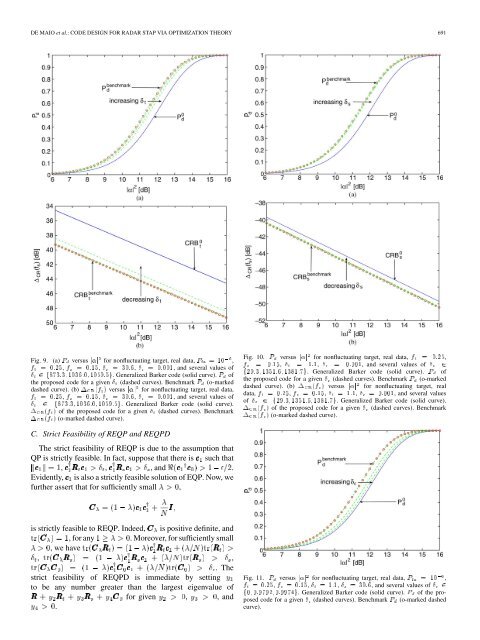
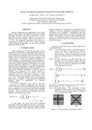
DE MAIO et al.: CODE DESIGN FOR RADAR STAP VIA OPTIMIZATION THEORY 691Fig. 9. (a) P versus jj for nonfluctuating target, real data, P = 10 ,f = 0:25, f = 0:15, = 30:6, = 0:001, and several values of 2 f873:3; 1036:0; 1059:5g. Generalized Barker code (solid curve). P ofthe proposed code for a given (dashed curves). Benchmark P (o-markeddashed curve). (b) 1 (f ) versus jj for nonfluctuating target, real data,f = 0:25, f = 0:15, = 30:6, = 0:001, and several values of 2 f873:3; 1036:0; 1059:5g. Generalized Barker code (solid curve).1 (f ) of the proposed code for a given (dashed curves). Benchmark1 (f ) (o-marked dashed curve).Fig. 10. P versus jj for nonfluctuating target, real data, f = 0:25,f = 0:15, = 1:1, = 0:001, and several values of 2f29:3; 1351:6; 1381:7g. Generalized Barker code (solid curve). P ofthe proposed code for a given (dashed curves). Benchmark P (o-markeddashed curve). (b) 1 (f ) versus jj for nonfluctuating target, realdata, f = 0:25, f = 0:15, = 1:1, = 0:001, and several valuesof 2 f29:3; 1351:6; 1381:7g. Generalized Barker code (solid curve).1 (f ) of the proposed code for a given (dashed curves). Benchmark1 (f ) (o-marked dashed curve).C. Strict Feasibility of REQP and REQPDThe strict feasibility of REQP is due to the assumption thatQP is strictly feasible. In fact, suppose that there is such that, , , and .Evidently, is also a strictly feasible solution of EQP. Now, wefurther assert that for sufficiently small ,is strictly feasible to REQP. Indeed, is positive definite, and, for any . Moreover, for sufficiently small,wehave, ,. Thestrict feasibility of REQPD is immediate by settingto be any number greater than the largest eigenvalue offor given , , and.Fig. 11. P versus jj for nonfluctuating target, real data, P = 10 ,f = 0:25, f = 0:15, = 1:1, = 30:6, and several values of 2f0; 0:9792; 0:9974g. Generalized Barker code (solid curve). P of the proposedcode for a given (dashed curves). Benchmark P (o-marked dashedcurve).
Page 1 and 2: IEEE TRANSACTIONS ON SIGNAL PROCESS
Page 3 and 4: DE MAIO et al.: CODE DESIGN FOR RAD
Page 5: DE MAIO et al.: CODE DESIGN FOR RAD
Page 8 and 9: 686 IEEE TRANSACTIONS ON SIGNAL PRO
Page 16: 694 IEEE TRANSACTIONS ON SIGNAL PRO

Code Design for Radar STAP via Optimization Theory

You also want an ePaper? Increase the reach of your titles

Delete template?

Save as template?