Code Design for Radar STAP via Optimization Theory

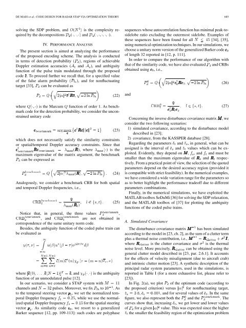
DE MAIO et al.: CODE DESIGN FOR RADAR STAP VIA OPTIMIZATION THEORY 685solving the SDP problem, and is the complexity requiredby the decompositions and .IV. PERFORMANCE ANALYSISThe present section is aimed at analyzing the performanceof the proposed encoding scheme. The analysis is conductedin terms of detection probability , regions of achievableDoppler estimation accuracies ( and ), and ambiguityfunction of the pulse train modulated through the proposedcode . To proceed further we recall that, for a specified valueof the false alarm probability , and for nonfluctuatingtarget [33], can be evaluated as(22)where is the Marcum function of order 1. As benchmarkcode for the detection probability, we consider the unconstrainedunitary code(23)which does not necessarily satisfy the similarity constraintsor spatial/temporal Doppler accuracy constraints. Since that, where is themaximum eigenvalue of the matrix argument, the benchmarkcan be expressed as(24)Analogously, we consider a benchmark CRB for both spatialand temporal Doppler frequencies, i.e.,(25)Notice that, in general, the three values ,, and are not obtained incorrespondence of the same unitary norm code.Besides, the ambiguity function of the coded pulse train canbe evaluated aswhere , and is the ambiguityfunction of an unmodulated pulse [12].In our scenario, we consider a STAP system withchannels and pulses. Moreover, we fix to .Asto the temporal steering vector , we set the normalized temporalDoppler frequency , while we use the normalizedspatial Doppler frequency for the spatial steeringvector . As similarity code , we resort to a generalizedBarker sequence [12, pp. 109-113]: such codes are polyphasesequences whose autocorrelation function has minimal peak-tosideloberatio excluding the outermost sidelobe. Examples ofthese sequences have been found for all [34], [35],using numerical optimization techniques. In our simulations, wechoose a unitary norm version of the generalized Barker codeof length 32 reported in [12, p. 111].In order to compare the performance of our algorithm withthat of the similarity code, we have also evaluated and CRBsobtained using , i.e.,and(26)(27)Concerning the inverse disturbance covariance matrix ,weconsider the two following scenarios:1) simulated covariance, according to the disturbance modeldescribed in [23];2) covariance, from the KASSPER database [28].Regarding the parameters and , in general, what can beassigned is the interval of and values which can be exploited.Evidently, they depend on , , and and must besmaller than the maximum eigenvalue of and respectively.From a practical point of view, the selection of the quotedparameters depend on the desired accuracy region (provided itis compatible with strict feasibility). In the numerical examples,we have considered a wide variation range for the parameters soas to better highlight the performance tradeoff due to differentparameters combinations.Finally, in the numerical simulations, we have exploited theMATLAB toolbox SeDuMi [36] for solving the SDP relaxation,and the MATLAB toolbox of [37] for plotting the ambiguityfunctions of the coded pulse trains.A. Simulated CovarianceThe disturbance covariance matrix has been simulatedaccording to the model in [23, ch. 2], as the sum of a clutter termplus a thermal noise contribution, i.e., ,where is the clutter covariance and is the thermalnoise level. More precisely, can be obtained using thegeneral clutter model described in [23, par. 2.6.1]. It accountsfor the effects of velocity misalignment (due to aircraft crab)and intrinsic clutter motion [23]. A synthetic description of theprincipal radar system parameters, used in the simulations, isreported in Table I (for a more exhaustive list, please refer to[23]).In Fig. 2(a), we plot of the optimum code (according tothe proposed criterion) versus for nonfluctuating target,, , and for several values of . In the samefigure, we also represent both the and the . Thecurves show that, increasing , we get lower and lower valuesof for a given value. This was expected since the higherthe smaller the feasibility region of the optimization problem