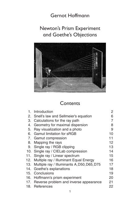
Newton's Prism Experiment and Goethe's Objections

Gernot Hoffmann
Newton’s Prism Experiment
and Goethe’s Objections
Contents
1. Introduction 2
2. Snell’s law and Sellmeier’s equation 6
3. Calculations for the ray path 7
4. Geometry for maximal dispersion 8
5. Ray visualization and a photo 9
6. Gamut limitation for sRGB 10
7. Gamut compression 11
8. Mapping the rays 12
9. Single ray / RGB clipping 13
10. Single ray / CIELab compression 14
11. Single ray / Linear spectrum 15
12. Multiple ray / Illuminant Equal Energy 16
13. Multiple ray / Illuminants A,D50,D65,D75 17
14. Goethe’s explanations 18
15. Conclusions 19
16. Hoffmann’s prism experiment 20
17. Reverse problem and inverse appearance 21
18. References 22
1

1.1 Introduction / How to use this doc
This document can be read by Adobe Acrobat. Some settings are essential: the color space
sRGB for the appearance; the resolution 72dpi for pixel synchronized images.
Best view zoom 200% (title image and photo on p.20).
Settings for Acrobat
Edit / Preferences / General / Page Display (since version 6)
Custom Resolution 72dpi
Edit / Preferences / General / Color Management (full version only)
sRGB
Euroscale Coated or ISO Coated or SWOP
Gray Gamma 2.2
A reasonable reproduction of the colors is possible only by a calibrated cathode ray tube
monitor or a high end LCD monitor (no hope for notebooks or laptops).
The monitor should be calibrated or adjusted by these test patterns:
CalTutor
http://www.fho-emden.de/~hoffmann/caltutor270900.pdf
Printing this doc accurately requires a calibrated printer, preferably an inkjet or high end color
laser printer. Office printers cannot reproduce the spectrum bars reasonably.
Accurate printing requires a calibrated printer
This document is protected by copyright. Any reproduction requires a permission by the author.
This should be considered as a protection against bad or wrong copying. The author provides
on demand files in RGB for the specific purpose in original quality and files for CMYK offset
printing (which cannot reproduce sRGB colors correctly), adjusted as good as possible.
Copyright
Gernot Hoffmann
August 2005
2

1.2 Introduction / About Newton
Isaac Newton lived from 1642 to 1727. His work about optics and color was probably inspired
by Descartes, Charleton, Boyle and Hook [5]. Refraction and dispersion by prisms were already
known at this time, but Newton introduced 1666 a set of three crucial experiments (in fact by
numerous experiments):
1. Refraction and dispersion of a thin ray, which produces a spectrum band with all rainbow
colors: red, orange, yellow, green, blue, indigo and violet.
2. Condensation of the spectrum band by a lens. This delivers again white light.
3. A spectral color, here a small part of the spectrum band, can be refracted again but it
cannot be further dispersed.
Indigo was added - though not visible - in order to get a ‘harmonic’ sequence like the seven
tones c,d,e,f,g,a,h,(c). The last tone c has double the frequency of the first. It is a strange
coincidence that this ratio is approximately valid for the frequencies or wavelengths of visible
light. In computer graphics we have a strong cyan between green and blue. In prism colors it
is sometimes detectable - a better candidate than indigo for the seventh rainbow color.
Newton’s theories were by no means always clear and understandable, which lead to lengthy
and often rather impolite discussions between the most famous scientists in Europe.
It is safe to say: Newton had discovered that white light consists of colored light.
Newton arranged the spectrum on a circle. Drawing by
the author, based on a print in Opticks [1].
Connecting the ends of a spectrum like this does not
have an equivalent for general electromagnetic or
acoustical waves.
This discovery was the first step towards spherical or
cylindrical three-dimensional color spaces [7], [24].
A segment of the circle is occupied by violet. Newton’s
violet is complementary to yellow-green.
In our present understanding this is mainly the magenta
segment, but magenta is mixed by red and blue (violet)
and not a spectral color.
Newton says: ’That if the point Z fall in or near to the line OD, the main ingredients being the
red and violet, the Colour compounded shall not be any of the prismatick Colours, but a
purple, inclining to red or violet, accordingly as the point Z lieth on the side of the line DO
towards E or towards C, and in general the compounded violet is more bright and more fiery
than the uncompounded’.
Newton knew already additive color mixing. He applied the center of gravity rule (which is
accurately valid in the CIE chromaticity diagram) in his wheel. Z is such a mixture.
The different refraction indices for different wavelengths lead Newton to the conclusion that
telescopes with mirrors instead of lens’ should be more accurate. He manufactured such a
telescope, using a metallic spherical mirror. The accuracy was probably affected by spherical
aberration. At that time it was assumed that an ideal mirror should have the shape of a cone
section but it was not yet discovered which one - a parabola. Manufacturing such a mirror
would have been impossible.
Newton published ’Opticks’ 1704, nearly forty years after his first experiments. In the time
between he had spent much time developing mathematical methods, geometry and principles
of mechanics.
3
D
Red
Violet
E
C
Orange
Z
Indigo
F
O
B
Yellow
Blew
G
A
Green

1.3 Introduction / About Goethe
Johann Wolfgang Goethe lived from 1749 to 1832. Well known as poet and writer, he was
familiar as well with philosophy and natural science.
1810 he published his book Geschichte der Farbenlehre [2]. This is mainly a historical review
but as well a furious attack against Newton’s theories. Judging by our actual understanding of
natural science, Goethe’s color theory was by no means well founded and elaborated. On the
other hand he tried to integrate the aspects of culture and art in his generalizing concepts.
The question remains: why did Goethe not believe in the Obvious in Newton’s theories ?
It is the purpose of this document to demonstrate that the obvious in our present understanding
was by no means obvious for Goethe. This demonstration will be done in an engineering
style, based on many illustrations. These are accurate in the sense of classical optics and in
the sense of actual color theory.
The author found during his Google search nearly nowhere correct illustrations for the prism
experiment. Drawings in publications are often wrong [5],[6], this could be a long list...
One of the best illustrations is the title graphic, dated 1912 [8], but even here rules fantasy
over reality: the blue-ish part is too small, indigo is in reality not perceivable and the geometrical
path of the red ray is not accurate.
4

1.4 Introduction / Goethe says...
Some statements by Goethe, important in our context, may be quoted [2], followed by a
simplified translation.
A [2, Zweiter Teil, Konfession des Verfassers ]
Aber wie verwundert war ich, als die durchs Prisma angeschaute weiße Wand nach wie vor
weiß blieb, daß nur da, wo ein Dunkles dran stieß, sich eine mehr oder weniger entschiedene
Farbe zeigte, daß zuletzt die Fensterstäbe am allerlebhaftesten farbig erschienen, indessen
am lichtgrauen Himmel draußen keine Spur von Färbung zu sehen war. Es bedurfte keiner
langen Überlegung, so erkannte ich, daß eine Grenze notwendig sei, um Farben hervorzubringen,
und ich sprach wie durch einen Instinkt sogleich vor mich laut aus, daß die Newtonische
Lehre falsch sei.’
’How surprised was I when I looked through a prism onto a white wall - still white, and colors
appeared only there where dark met white. It was immediately clear that colors can appear
only at boundaries. And I said loud, guided by an instinct: Newton’s teaching is wrong.’
B [2, Zweiter Teil, Polemischer Teil ]
’Also, um beim Refraktionsfalle zu verweilen, auf welchem sich die Newtonische Theorie
doch eigentlich gründet, so ist es keineswegs die Brechung allein, welche die Farbenerscheinung
verursacht; vielmehr bleibt eine zweite Bedingung unerläßlich, daß nämlich die
Brechung auf ein Bild wirke und ein solches von der Stelle wegrücke.
Ein Bild entsteht nur durch seine Grenzen; und diese Grenzen übersieht Newton ganz, ja er
leugnet ihren Einfluß...und keines Bildes Mitte wird farbig, als insofern die farbigen Ränder
sich berühren oder übergreifen.’
’Again about the refraction, which is the true basis of Newton’s theory: color effects are not
generated by refraction alone. A second necessary condition is, that refraction acts on an
image by shifting it. An image is created merely by its boundaries, and these boundaries are
not taken into account by Newton... and no image will become colorful in the middle, unless
the colored boundaries touch or overlap each other.’
C [2, Zweiter Teil, Beiträge zur Optik ]
’Unter den eigentlichen farbigen Erscheinungen sind nur zwei, die uns einen ganz reinen
Begriff geben, nämlich Gelb und Blau. Sie haben die besondere Eigenschaft, daß sie zusammen
eine dritte Farbe hervorbringen, die wir Grün nennen.
Dagegen kennen wir die rote Farbe nie in einem ganz reinen Zustande: denn wir finden, daß
sie sich entweder zum Gelben oder zum Blauen hinneigt.’
’Only two colors can be considered as pure: yellow and blue. Their special feature is: they
generate together a new color which we call green. Red is never pure: we find that this color
tends either to yellow or to blue.’
5

2. Snell’s law and Sellmeier’s equation
The refraction of a ray which enters from a medium with refraction index n 1 into a medium with
refraction index n 2 is defined by Snell’s law.
The angles α and β are shown on the next page.The refraction index for air is practically 1.0.
sin( b)
n1
1
= =
sin( a ) n2n Goethe said: Willebrord Snellius (1591-1626) knew the fundamentals but he did not know the
definition by sine functions [2, Erster Teil, Fünfte Abteilung ].
The refraction index as a function of the wavelength can be modelled by Sellmeier’s equation:
2 B1
n
C
2
l
( l)
= 1+
2
l -
1.80
n
1.75
1.70
1.65
1.60
1.55
1
2
B2
l
+
2
l - C
2
SF15
BK7
1.50
0.3 0.4 0.5 0.6 0.7 λ / µ m 0.8
2
B3
l
+
2
l - C
3
The structure of this function is essentially based on Maxwell’s theory of continua [4]. The
function has three poles which are outside the spectrum of visible light. The poles indicate
resonance phenomena without damping. In reality the peaks are finite because of damping.
The actual parameters are found by measurements, here for special types of flint and crown
glass.
The refraction of flint glass is stronger. Because of the steeper slope the dispersion is stronger
as well. Combinations of flint glass and crown glass can be used for achromatic lens or prism
systems which show no dispersion for two distinct wavelengths and nearly no dispersions for
the others. Goethe knew this already.
Tables are supplied by Schott AG [15], here used for flint glass SF15. Thanks to Danny Rich.
The Sellmeier equation and the data for crown glass BK7 were found at Wikipedia [16].
6
Glass SF15
B1 1.539259
B2 0.247621
B3 1.038164
C1 0.011931
C2 0.055608
C3 116.416755
Glass BK7
B1 1.039612
B2 0.231792
B3 1.010469
C1 0.006001
C2 0.020018
C3 103.560653

3. Calculations for the ray path
The path of the ray is calculated by intersections of line segments, using Snell’s law and some
simple geometry: lines in parametric representation; solutions by Cramer’s rule. All direction
vectors are normalized for unit length. The origin of u 1 is at C 1 .
� 1
R1 C1 u1 n1 d1 g1
=
È - sin( g)
˘
ÎÍ + cos( g)
˚˙
u1
=
È - sin( r1)
˘
ÎÍ - cos( r1)
˚˙
d1
=
È+
cos( r 1)
˘
ÎÍ - sin( r1)
˚˙
r1 = c1+ uu1
x1 = r1+ l d1
x2 = m g1
x1 = x2
mg1 - ld1
= r1
m g1x - l d1x = r1x
mg - ld
= r
1y 1y 1y
� 1
Solution by Cramer’s rule
dA = d1xg1y - d g
dM = d1 r1 -d1
r1
m = dM/ dA
p1 = m g1
a = g + r
1 1
1y 1x
x y y x
Refraction by Snell’s law
sin( b ) = ( 1/
n)sin(
a )
1 1
P 1
cos( b1) = 1-sin
( b1)
b1
= a tan2
[sin( b1),cos( b1)]
d = g -b
1 1
2
d 0
� 1
g 1
�
y
g 2
7
� 2
P 2
d2 �2 � 2
C 2
u 2
n 2
g2
=
È + sin( g)
˘
ÎÍ + cos( g)
˚˙
d0
=
È+
cos( d1)
˘
ÎÍ + sin(
d1)
˚˙
x1 = p1+ l d0
x2
= m g2
dA = d g -d
g
dM = d p -d
p
p2 = ( dM/ dA)
g2
b2= g + d
sin( a ) = n sin( b )
2 2
n 1.5500
rho1 45.0000
rho2 45.0000
alf1 75.0000
bet1 38.5486
alf2 34.5311
bet2 21.4514
defl 49.5311
x
R 2
0x 2y 0y 2x
0x 1y 0y 1x
cos( a2) = 1-sin
( a2)
a = atan
2 [ sin( a ),cos( a )]
2 2 2
u2
=
È + sin( r2)
˘
ÎÍ - cos( r2)
˚˙
d2 = a2 -g
d2
=
È+
cos( d2
) ˘
ÎÍ + sin( d2
) ˚˙
x1 = p2 + l d2
x2 = c2 + mu2
s2 = p2 -c2
dA = d u -d
u
dM = d s -d
s
2
2x 2y 2y 2x
2x 2y 2y 2x
r = c +( dM/ dA)
u
2 2 2

4. Geometry for maximal dispersion
For a practical prism experiment the dispersion should be as large as possible. Flint glass is
the better choice. The optimal angles can be found by trial and error.
The simulation below confirms the test results. Left crown glass, right flint glass.The upper
two images show the symmetrical case. The lower show the optimal case.The output angle β 2
should be near to 90° for the shortest wavelength (violet).
In the middle images one can see that large input angles α 1 do not deliver the best results.
Glass BK7
LBlue 0.3800
LRed 0.7000
nBlue 1.5337
nRed 1.5131
rho1 20.0000
rho2 20.0000
For blue
alf1 50.0000
bet1 29.9643
alf2 50.1478
bet2 30.0357
defl 40.1478
disp 1.8184
Glass BK7
LBlue 0.3800
LRed 0.7000
nBlue 1.5337
nRed 1.5131
rho1 52.0000
rho2 0.0000
For blue
alf1 82.0000
bet1 40.2147
alf2 31.2764
bet2 19.7853
defl 53.2764
disp 1.5672
Glass BK7
LBlue 0.3800
LRed 0.7000
nBlue 1.5337
nRed 1.5131
rho1 1.0000
rho2 55.0000
For blue
alf1 31.0000
bet1 19.6215
alf2 83.5210
bet2 40.3785
defl 54.5210
disp 6.4668
Crown glass Flint glass
8
Glass SF15
LBlue 0.3800
LRed 0.7000
nBlue 1.7548
nRed 1.6890
rho1 31.4000
rho2 31.0000
For blue
alf1 61.4000
bet1 30.0221
alf2 61.2600
bet2 29.9779
defl 62.6600
disp 7.1119
Glass SF15
LBlue 0.3800
LRed 0.7000
nBlue 1.7548
nRed 1.6890
rho1 55.0000
rho2 19.0000
For blue
alf1 85.0000
bet1 34.5899
alf2 48.8484
bet2 25.4101
defl 73.8484
disp 5.7646
Glass SF15
LBlue 0.3800
LRed 0.7000
nBlue 1.7548
nRed 1.6890
rho1 19.0000
rho2 55.0000
For blue
alf1 49.0000
bet1 25.4729
alf2 84.0482
bet2 34.5271
defl 73.0482
disp 15.4286

5. Ray visualization and a photo
We are using throughout the document wavelengths from 0.380µm to 0.700µm. This range
reaches from nearly invisible violet to nearly invisible red. The colors at the end of the spectrum
can be made visible only by rather strong light sources in laboratories, 0.360µm to 0.800µm.
A crude color visualization approximation is achieved by nonlinear HSB, a modification of the
standard Hue-Saturation-Brightness model, which is represented by a cone [9], [24].
This is a photo of a real spectrum bar. A little image processing was applied.
9
Glass SF15
LBlue 0.3800
LRed 0.7000
nBlue 1.7548
nRed 1.6890
rho1 19.0000
rho2 54.0000
For blue
alf1 49.0000
bet1 25.4729
alf2 84.0482
bet2 34.5271
defl 73.0482
disp 15.4286

6. Gamut limitation for sRGB
A correct visualization of the calculated spectrum bar would require media which can reproduce
all spectral colors. This is not possible, not even by lasers. Especially one needs a plausible
color reproduction on common cathode ray tube monitors (CRT monitors).
The chromaticity diagram CIE xyY below is a special perspective projection of the physical
color space CIE XYZ onto a plane. The area, filled symbolically by colors, represents the
human gamut, but the luminance is left out. Spectral colors are on the horseshoe contour.
The magenta line shows mixtures of violet and red. Magenta itself is not a spectral color.
The magenta line is practically a fiction because the end points are nearly invisible in real life.
Practical magentas are mixed by blue and red.
Inside the horseshoe contour is the gamut triangle for sRGB (Rec.709 primaries and D65
white point), but this triangle is the projection of an affine distorted cube. The gamut depends
on the luminance as well, which is shown for increasing luminances Y=0.05 to 0.95 [22],[23].
sRGB is a standardized color space, a reasonable model for real CRT monitors. Mapping
spectral colors to sRGB is obviously very difficult. Especially vibrant oranges are missing.
1.0
y
0.9
0.8
0.7
0.6
0.5
0.4
0.3
0.2
0.1
520 525
515 530
535
510
540
545
550
505
555
560
565
500
570
575
580
585
495
590
595
490
0.95
0.85
0.75
0.65
0.55
0.45
600
605
610
620
635
700
485 0.35
0.25
480
0.15
475
470
0.05
460
380
Magenta line
0.0
0.0 0.1 0.2 0.3 0.4 0.5 0.6 0.7 0.8 0.9 x 1.0
10

7. Gamut compression
7.1 Gamut compression Type A for single ray spectra in CIELab
If the spectrum is generated by one ray, then the visualization by sRGB requires optimally
saturated colors and a certain visual balance as well.
If an orange cannot be shown brightly, then it is less convenient to show yellow in the neighbourhood
as bright as possible.
The blue part looks always too bright. This well-known phenomenon will be explained later.
The gamut compression is done in CIELab [10],[21] by the author’s simple method. More
subtle strategies for gamut compressions are described e.g. by Ján Morovic [14].
Find the hue in Lab by a,b (asterisks L*.. omitted)
Reduce the radius towards the L-axis until R,G,B
are in-gamut
This delivers a 1,b 1,L1 Modify L by
L 2 = 0.5 + 0.7(L-0.5)
Reduce the radius towards the L-axis until R,G,B
are in-gamut
This delivers a 2,b 2,L2 Apply a linear interpolation between 1 and
2 and
find the position with maximal saturation
s = a 2 + b 2 /L
7.2 Gamut compression Type B for multiple ray spectra in CIELab
The complete compression as above is not useful for spectra which are generated by several
rays. In this case the light in the middle is more or less white and an increased saturation
would be wrong.
The Lab luminance is simply multiplied by a factor of about 0.95 and only the first step of the
compression is executed.
7.3 Gamut compression Type C by RGB clipping
Crude RGB clipping - even proportional clipping like here - does not deliver pleasant results.
If R

8. Mapping the rays
The upper image shows again the crude color approximation by nonlinear HSB, now with a
smaller number of color rays.
The lower image shows the content of an array with 1000+1 elements on the screen (right
plane), starting approximately at the origin. Each color ray hits an element of this array.
The wavelength is written into the array. Gaps are filled by linear interpolation.
At position R we have many color rays per length, at position V fewer. In order to distribute the
energy correctly across the length, the array content is multiplied by a slope factor. This is
calculated by a linear interpolation of the slopes between sV and sR.
The content of the array is converted into the color space CIE XYZ, using the common colormatching
functions, and then converted to sRGB [10],[21],[22].
Compression is here done by Type C, RGB clipping. The spectrum bar is shown banded.
0.70
0.66
0.62
0.58
0.54
0.50
0.46
0.42
0.38
λ / µ m
sV
0 1000
12
V
R
sR
Glass SF15
LBlue 0.3800
LRed 0.7000
nBlue 1.7548
nRed 1.6890
rho1 19.0000
rho2 54.0000
For blue
alf1 49.0000
bet1 25.4729
alf2 84.0482
bet2 34.5271
defl 73.0482
disp 15.4286

9. Single ray / Illuminant Equal Energy / Compr. Type C / RGB clipping
Illuminant Equal Energy has a flat spectrum. Compression is done by Type C, RGB clipping.
The spectrum bars are shown banded and continuous. The table shows linear RGB values,
the bars were calculated with gamma encoding for sRGB. RGB clipping does not create
balanced distributions of colors.
No RGB clipping, no RGB gamma encoding
Lam L* a* b* R G B
0.38 0.0 5.5 -9.2 0.3 -0.3 1.8
0.39 0.1 16.9 -25.0 0.9 -0.8 5.5
0.40 0.4 53.0 -51.1 3.0 -2.6 18.5
0.41 1.1 105.2 -85.6 9.1 -8.0 56.5
0.42 3.6 175.9 -134.2 27.4 -24.5 175.7
0.43 10.3 221.0 -171.4 53.9 -49.9 376.9
0.44 17.0 215.6 -177.2 56.7 -56.6 474.6
0.45 23.0 185.5 -168.0 37.6 -46.1 480.4
0.46 29.4 141.2 -152.3 4.6 -25.5 450.9
0.47 36.2 70.2 -121.5 -37.9 8.9 345.1
0.48 44.1 -26.5 -77.8 -78.8 51.5 213.2
0.49 52.7 -134.8 -32.1 -114.2 96.5 115.0
0.50 63.6 -254.0 11.3 -157.2 156.2 56.6
0.51 76.3 -290.7 53.9 -209.6 240.0 16.6
0.52 87.5 -243.4 95.3 -236.0 324.8 -14.9 0.53 94.4 -196.6 122.7 -206.5 371.9 -31.1 0.54 98.2 -155.4 143.9 -136.6 384.8 -40.0 0.55 99.8 -114.3 159.6 -32.9 368.9 -43.2 0.56 99.8 -71.6 166.5 100.8 329.1 -42.3 0.57 98.1 -27.4 166.2 256.4 267.1 -38.1 0.58 94.7 16.6 161.0 416.0 189.7 -31.8 0.59 89.7 57.3 153.1 551.3 108.5 -24.5 0.60 83.5 90.0 142.8 630.4 39.3 -17.5 0.61 76.3 111.3 131.0 631.4 -7.2 -11.8 0.62 68.1 120.1 117.1 556.8 -28.9 -7.6
0.63 58.5 117.6 100.8 427.0 -32.0 -4.7
0.64 48.9 109.4 84.3 301.6 -27.0 -2.7
0.65 39.1 96.7 67.4 192.4 -18.9 -1.5
0.66 29.7 82.0 51.1 112.4 -11.6 -0.8
0.67 20.8 66.9 35.9 59.7 -6.3 -0.4
0.68 13.8 54.7 23.8 32.0 -3.4 -0.2
0.69 7.4 43.1 12.8 15.5 -1.7 -0.1
0.70 3.7 29.5 6.4 7.8 -0.9 -0.1
0.70
0.66
0.62
0.58
0.54
0.50
0.46
0.42
0.38
λ / µ m
13
With RGB clipping, no RGB gamma encoding
Lam L* a* b* R G B
0.38 0.7 4.2 -8.2 0.3 0.0 1.8
0.39 2.1 12.9 -22.0 0.9 0.0 5.5
0.40 7.0 34.1 -40.1 3.0 0.0 18.5
0.41 17.3 49.7 -58.4 9.1 0.0 56.5
0.42 32.4 72.4 -85.6 27.4 0.0 175.7
0.43 40.8 83.1 -93.5 53.9 0.0 255.0
0.44 41.1 83.3 -92.9 56.7 0.0 255.0
0.45 38.5 81.8 -97.4 37.6 0.0 255.0
0.46 33.1 79.5 -106.4 4.6 0.0 255.0
0.47 37.3 64.0 -99.5 0.0 8.9 255.0
0.48 52.4 13.7 -64.0 0.0 51.5 213.2
0.49 61.9 -30.4 -17.2 0.0 96.5 115.0
0.50 73.2 -60.1 26.0 0.0 156.2 56.6
0.51 85.9 -81.4 67.1 0.0 240.0 16.6
0.52 87.7 -86.2 83.2 0.0 255.0 0.0
0.53 87.7 -86.2 83.2 0.0 255.0 0.0
0.54 87.7 -86.2 83.2 0.0 255.0 0.0
0.55 87.7 -86.2 83.2 0.0 255.0 0.0
0.56 91.6 -54.9 87.9 100.8 255.0 0.0
0.57 97.1 -21.6 94.5 255.0 255.0 0.0
0.58 89.1 -6.4 88.7 255.0 189.7 0.0
0.59 77.1 19.0 80.4 255.0 108.5 0.0
0.60 63.6 51.7 72.0 255.0 39.3 0.0
0.61 53.2 80.1 67.2 255.0 0.0 0.0
0.62 53.2 80.1 67.2 255.0 0.0 0.0
0.63 53.2 80.1 67.2 255.0 0.0 0.0
0.64 53.2 80.1 67.2 255.0 0.0 0.0
0.65 47.0 72.9 61.2 192.4 0.0 0.0
0.66 36.7 60.9 51.1 112.4 0.0 0.0
0.67 26.7 49.4 39.5 59.7 0.0 0.0
0.68 18.7 40.1 28.7 32.0 0.0 0.0
0.69 11.2 31.5 17.7 15.5 0.0 0.0
0.70 5.9 24.1 9.3 7.8 0.0 0.0

10. Single ray / Illuminant Equal Energy / Compr. Type A / CIELab
The same method as in the previous chapter, but now the compression is done by Type A in
CIELab. The spectrum bars look better balanced.The table shows linear RGB values, the
bars were calculated with gamma encoding for sRGB.The spectrum bars look better balanced
because of CIELab gamut compression.
No gamut compression, no RGB gamma encoding
Lam L* a* b* R G B
0.38 0.0 5.5 -9.2 0.3 -0.3 1.8
0.39 0.1 16.9 -25.0 0.9 -0.8 5.5
0.40 0.4 53.0 -51.1 3.0 -2.6 18.5
0.41 1.1 105.2 -85.6 9.1 -8.0 56.5
0.42 3.6 175.9 -134.2 27.4 -24.5 175.7
0.43 10.3 221.0 -171.4 53.9 -49.9 376.9
0.44 17.0 215.6 -177.2 56.7 -56.6 474.6
0.45 23.0 185.5 -168.0 37.6 -46.1 480.4
0.46 29.4 141.2 -152.3 4.6 -25.5 450.9
0.47 36.2 70.2 -121.5 -37.9 8.9 345.1
0.48 44.1 -26.5 -77.8 -78.8 51.5 213.2
0.49 52.7 -134.8 -32.1 -114.2 96.5 115.0
0.50 63.6 -254.0 11.3 -157.2 156.2 56.6
0.51 76.3 -290.7 53.9 -209.6 240.0 16.6
0.52 87.5 -243.4 95.3 -236.0 324.8 -14.9 0.53 94.4 -196.6 122.7 -206.5 371.9 -31.1 0.54 98.2 -155.4 143.9 -136.6 384.8 -40.0 0.55 99.8 -114.3 159.6 -32.9 368.9 -43.2 0.56 99.8 -71.6 166.5 100.8 329.1 -42.3 0.57 98.1 -27.4 166.2 256.4 267.1 -38.1 0.58 94.7 16.6 161.0 416.0 189.7 -31.8 0.59 89.7 57.3 153.1 551.3 108.5 -24.5 0.60 83.5 90.0 142.8 630.4 39.3 -17.5 0.61 76.3 111.3 131.0 631.4 -7.2 -11.8 0.62 68.1 120.1 117.1 556.8 -28.9 -7.6
0.63 58.5 117.6 100.8 427.0 -32.0 -4.7
0.64 48.9 109.4 84.3 301.6 -27.0 -2.7
0.65 39.1 96.7 67.4 192.4 -18.9 -1.5
0.66 29.7 82.0 51.1 112.4 -11.6 -0.8
0.67 20.8 66.9 35.9 59.7 -6.3 -0.4
0.68 13.8 54.7 23.8 32.0 -3.4 -0.2
0.69 7.4 43.1 12.8 15.5 -1.7 -0.1
0.70 3.7 29.5 6.4 7.8 -0.9 -0.1
0.70
0.66
0.62
0.58
0.54
0.50
0.46
0.42
0.38
λ / µ m
14
With gamut compression, no RGB gamma encoding
Lam L* a* b* R G B
0.38 0.0 0.2 -0.3 0.0 0.0 0.1
0.39 0.1 0.7 -1.0 0.1 0.0 0.2
0.40 0.4 2.0 -1.9 0.3 0.0 0.5
0.41 1.1 5.8 -4.7 1.1 0.0 1.2
0.42 3.6 18.9 -14.5 3.4 0.0 4.0
0.43 10.3 34.9 -27.1 9.3 0.0 13.6
0.44 17.0 44.4 -36.5 17.7 0.0 29.3
0.45 23.0 53.6 -48.5 26.7 0.0 56.1
0.46 29.4 65.6 -70.8 31.3 0.0 120.3
0.47 36.2 49.8 -86.3 0.0 12.5 198.2
0.48 44.1 -10.4 -30.7 0.1 41.1 83.3
0.49 51.9 -31.5 -7.5 0.0 65.3 62.5
0.50 59.5 -41.0 1.8 0.0 91.7 65.8
0.51 68.4 -49.5 9.2 0.1 129.5 76.2
0.52 76.2 -60.7 23.8 0.2 172.3 68.8
0.53 81.1 -71.9 44.9 0.0 204.8 41.5
0.54 83.7 -82.3 76.1 0.0 226.4 3.7
0.55 84.9 -58.9 82.2 62.6 215.8 0.0
0.56 84.9 -35.6 82.9 128.8 196.1 0.3
0.57 83.7 -13.8 83.6 191.4 169.3 0.0
0.58 81.3 8.5 82.8 250.6 136.0 0.3
0.59 77.8 20.9 56.0 255.0 110.1 24.2
0.60 73.4 31.0 49.2 254.5 85.1 26.4
0.61 68.4 42.2 49.7 254.3 59.7 19.4
0.62 62.7 55.6 54.3 254.9 34.4 10.2
0.63 56.0 72.7 62.3 254.9 9.1 2.3
0.64 49.2 75.8 58.4 213.4 0.0 1.5
0.65 39.1 63.8 44.4 127.5 0.0 2.1
0.66 29.7 53.4 33.3 72.9 0.0 2.0
0.67 20.8 43.0 23.1 37.9 0.0 1.6
0.68 13.8 34.7 15.1 19.9 0.0 1.2
0.69 7.4 27.3 8.1 9.6 0.0 0.7
0.70 3.7 17.2 3.7 4.8 0.0 0.4

11. Single Ray / Linear Spectrum / Illuminant Equal Energy /
Compr. Type A / CIELab
This is not the prism experiment. The wavelength is now linearly distributed along the horizontal
axis. Graphics like this appear often in text books, mostly wrong though.
Modern spectrophotometers use gratings instead of prisms.Then the bar would look like here.
The table shows linear RGB values. Instead of Lab values (the same as on the previous page)
the CIE XYZ values are shown. The bars were calculated with gamma encoding for sRGB.
No gamut compression, no RGB gamma encoding
Lam X 100 Y 100 Z 100 R G B
0.38 0.1 0.0 0.6 0.3 -0.3 1.8
0.39 0.4 0.0 2.0 0.9 -0.8 5.5
0.40 1.4 0.0 6.8 3.0 -2.6 18.5
0.41 4.4 0.1 20.7 9.1 -8.0 56.5
0.42 13.4 0.4 64.6 27.4 -24.5 175.7
0.43 28.4 1.2 138.6 53.9 -49.9 376.9
0.44 34.8 2.3 174.7 56.7 -56.6 474.6
0.45 33.6 3.8 177.2 37.6 -46.1 480.4
0.46 29.1 6.0 166.9 4.6 -25.5 450.9
0.47 19.5 9.1 128.8 -37.9 8.9 345.1
0.48 9.6 13.9 81.3 -78.8 51.5 213.2
0.49 3.2 20.8 46.5 -114.2 96.5 115.0
0.50 0.5 32.3 27.2 -157.2 156.2 56.6
0.51 0.9 50.3 15.8 -209.6 240.0 16.6
0.52 6.3 71.0 7.8 -236.0 324.8 -14.9 0.53 16.5 86.2 4.2 -206.5 371.9 -31.1 0.54 29.0 95.4 2.0 -136.6 384.8 -40.0 0.55 43.3 99.5 0.9 -32.9 368.9 -43.2 0.56 59.4 99.5 0.4 100.8 329.1 -42.3 0.57 76.2 95.2 0.2 256.4 267.1 -38.1 0.58 91.6 87.0 0.2 416.0 189.7 -31.8 0.59 102.6 75.7 0.1 551.3 108.5 -24.5 0.60 106.2 63.1 0.1 630.4 39.3 -17.5 0.61 100.3 50.3 0.0 631.4 -7.2 -11.8 0.62 85.4 38.1 0.0 556.8 -28.9 -7.6
0.63 64.2 26.5 0.0 427.0 -32.0 -4.7
0.64 44.8 17.5 0.0 301.6 -27.0 -2.7
0.65 28.3 10.7 0.0 192.4 -18.9 -1.5
0.66 16.5 6.1 0.0 112.4 -11.6 -0.8
0.67 8.7 3.2 -0.0 59.7 -6.3 -0.4
0.68 4.7 1.7 0.0 32.0 -3.4 -0.2
0.69 2.3 0.8 -0.0 15.5 -1.7 -0.1
0.70 1.1 0.4 -0.0 7.8 -0.9 -0.1
0.70
0.66
0.62
0.58
0.54
0.50
0.46
0.42
0.38
λ / µ m
15
With gamut compression, no RGB gamma encoding
Lam X 100 Y 100 Z 100 R G B
0.38 0.0 0.0 0.0 0.0 0.0 0.1
0.39 0.0 0.0 0.1 0.1 0.0 0.2
0.40 0.1 0.0 0.2 0.3 0.0 0.5
0.41 0.3 0.1 0.5 1.1 0.0 1.2
0.42 0.8 0.4 1.5 3.4 0.0 4.0
0.43 2.5 1.2 5.2 9.3 0.0 13.6
0.44 4.9 2.3 11.1 17.7 0.0 29.3
0.45 8.3 3.8 21.1 26.7 0.0 56.1
0.46 13.6 6.0 45.1 31.3 0.0 120.3
0.47 15.8 9.1 74.5 0.0 12.5 198.2
0.48 11.7 13.9 33.0 0.1 41.1 83.3
0.49 13.6 20.1 26.3 0.0 65.3 62.5
0.50 17.5 27.6 28.8 0.0 91.7 65.8
0.51 23.6 38.5 34.5 0.1 129.5 76.2
0.52 29.1 50.3 33.7 0.2 172.3 68.8
0.53 31.7 58.6 25.0 0.0 204.8 41.5
0.54 32.0 63.6 12.0 0.0 226.4 3.7
0.55 40.4 65.7 10.6 62.6 215.8 0.0
0.56 48.3 65.7 10.3 128.8 196.1 0.3
0.57 54.7 63.5 9.4 191.4 169.3 0.0
0.58 59.6 59.0 8.4 250.6 136.0 0.3
0.59 58.4 52.8 16.1 255.0 110.1 24.2
0.60 55.0 45.8 15.7 254.5 85.1 26.4
0.61 50.9 38.5 12.0 254.3 59.7 19.4
0.62 46.8 31.2 7.3 254.9 34.4 10.2
0.63 42.7 23.9 3.2 254.9 9.1 2.3
0.64 34.6 17.8 2.2 213.4 0.0 1.5
0.65 20.8 10.7 1.8 127.5 0.0 2.1
0.66 11.9 6.1 1.3 72.9 0.0 2.0
0.67 6.3 3.2 0.9 37.9 0.0 1.6
0.68 3.3 1.7 0.6 19.9 0.0 1.2
0.69 1.6 0.8 0.3 9.6 0.0 0.7
0.70 0.8 0.4 0.2 4.8 0.0 0.4

12. Multiple ray / Illuminant Equal Energy / Compr. Type B / CIELab
A continuous light band with flat spectrum is simulated by multiple rays. Each of them is interpreted
according to chapter 8. The content of the interpolated measurement array is multiplied
by the color-matching functions and the slope function. Then summed up in a second array
which contains CIE XYZ values for each wavelength. The content of the XYZ array is normalized
for Ymax =1 after finishing the measurement. The sum approximates an integration.
In the middle we have white light. At the ends we can see color fringes. This is Goethe’s
important observation on which he based his attack against Newton: colors appear at the
boundaries of light and shadow.
0.70
0.66
0.62
0.58
0.54
0.50
0.46
0.42
0.38
λ / µ m
0 1000
Illuminant Equal Energy
16

13. Multiple ray / Illuminants A, D50, D65,D75 / Compr. Type B / CIELab
Different illuminants generate different shades of white in the middle. Illuminant A is a Planckian
radiator with color temperature 2856K, as produced by a domestic tungsten bulb. Candle
light would look even ‘warmer’, which means it has a lower color temperature, about 1900K.
Graphics for typical spectra are found in books [10] and in documents by the author [19].
The values in the measurement array are multiplied by one of these spectra as well, in addition
to the multiplication by color-matching functions and slope functions.
In real life the discrepancies for different illuminants would be less obvious because of
adaptation: the tungsten or candle yellow would look less yellow-ish and north skylight D75
would look less blue-ish.
The simulation of perceived colors is handled in color theory by chromatic adaptation transforms
[10],[14],[21]. These are not applied here.
0.70
0.66
0.62
0.58
0.54
0.50
0.46
0.42
0.38
λ / µ m
0 1000
Illuminant A
Illuminant D50
Illuminant D65
Illuminant D75
17

14. Goethe’s explanations
The graphic shows Goethe’s Fünfte Tafel. Here it is a new drawing by the author, based on a
print in [2], as accurate as possible.
The small image top left visualizes three situations for a light band, represented by two rays:
without refraction, refracted by a parallel plate and refracted by the upper prism. Color fringes
are emphasized. The large image should make the refraction effect by one prism much clearer.
The ray geometry in the prism (A) is wrong, but this is more a symbolical drawing which
shows ’light versus shadow’.
The cross-section (B) is approximately the same as in the previous chapters. But then said
Goethe: ’the cross-section, where the ellipse is drawn, is about the one where Newton and his
followers perceive, fix and measure the image’.
Does it mean that Goethe expected a spectrum without white in the middle, like in the crosssections
(C) to (E) ? Just an overlay of edge effects ? It seems so, but then he were terribly
wrong - the rays in the middle cannot be ignored.
Goethe used a light band, Newton used for his crucial experiments a thin ray. And he knew
already that light bands deliver white in the middle.
18
A
B
C
D
E

15. Conclusions
The Conclusions refer to the Introduction, chapter 1. Furtheron some remarks on the perceived
brightness of blue are added.
A [2, Zweiter Teil, Konfession des Verfassers ]
Aber wie verwundert war ich, ...’
A prism refracts a light band or a dense bundle of (fictitious) rays without strong color effects
in the middle because these rays sum up to white light. Goethe was not aware of this superposition.
Therefore he emphasized color effects correctly at the boundary of the bundle.
Newton’s crucial experiments were essentially done with thin rays.
It is not understandable why Goethe did not discuss the case for a thin ray. It seems that he
regarded this as a quite unnatural test condition which had nothing to do with real life.
In fact he did not read Opticks carefully or at all. For example, the ellipse (C) in his drawing
was clearly described by Newton as ‘oblong’, the envelop of a sequence of circles.
B [2, Zweiter Teil, Polemischer Teil ]
’Also, um beim Refraktionsfalle zu verweilen, ...’
Goethe assumes that refraction itself does not create color effects. This would require an
image which is refracted and shifted as well, and which has boundaries, because it is an
image. But if it is refracted then it is shifted - the argument is not understandable.
On the other hand he is right in a certain sense, though without being aware of: refraction
itself does not colorize anything. The color or dispersion is a result of different refraction
indices for different wavelengths, for different spectral colors.
C [2, Zweiter Teil, Beiträge zur Optik ]
’Unter den eigentlichen farbigen Erscheinungen sind nur zwei, ...’
Goethe’s Erste Tafel shows color wheels. He had accepted Newton’s model to a certain extent.
Goethe’s model uses (also according to [7]) three primaries yellow, blue, red and three
secondaries orange, violet, green. On the other hand he considers only yellow and blue as
pure colors. Maybe this was just an unnecessary complication.
Goethe knew almost all the other contributors to color science, as mentioned in the same
book [7], but not yet Philipp Otto Runge, who published 1810 the first threedimensional color
space, a sphere.
The Blue Mystery
In simulations we perceive in the spectrum bars the small part for pure blue on monitors as
too bright. The color reproduction is based on the sRGB model which describes with sufficient
accuracy common cathode ray tube monitors (real monitors are calibrated by instruments, a
process which introduces the actual parameters into the color management system).
The contribution of blue to the luminance is given by equations like this:
L = 0.3R + 0.6G + 0.1B
With accurate numbers this is colorimetrically correct. Is blue really six or seven times darker
than green ? The author could not prove such a ratio by flicker tests.
An explanation might be the Helmholtz-Kohlrausch effect [13] which means: fully saturated
colors appear brighter than less saturated colors. The table in chapter 10 shows the highest
saturations for red at 0.63µm, for green at 0.54µm and for blue at 0.47µm.
19

16. Hoffmann’s prism experiment
A slide projector is used as light source. The slide is a metal plate with a thin horizontal slit.
The cylinder with the prism can be rotated. The spectrum bar appears on an adjustable glass
plate which is ground on one side. The mechanical system can be folded and stored together
with the projector in a suitcase. A student’s project by Mr. Burhan Primanintyo.
Best view zoom 200%.
20

17. Reverse problem and inverse appearance
In September 2012 the author received a message by Dr.Stephen R.J.Williams, a UK-based
Geo-scientist:
The images in your chapter 12 seem to explain how the fringes are produced. My interpretation
(see attached illustration) of your diagram indicates that observer will see blue
fringes at top of aperture image and red/yellow fringes at bottom of aperture image.
But when I look through a real prism I see blue fringes at the bottom of the aperture
image and red/yellow fringes at the top. This is opposite to that in the diagram.
Dr.Williams is right. Later he provided the link [26], which is of high value. But this report does
not explain the problem in a convincing manner, does not explain what is called below the
inverse appearance phenomenon.
Not even Goethe himself had described the discrepancy between his drawing Fünfte Tafel in
chapter 14 and his view through the prism. The drawing reproduces more or less Newton‘s
approach (with some errors though, concerning the angles of refraction). It shows the color
bands on a screen, similar to all the other illustrations here in this document.
Looking through a prism is in [26] called the reverse problem - exactly Goethe‘s approach, but
not in his drawing. The inversion, as observed by Dr.Williams, is here called inverse appearance
phenomenon.
The explanation follows Dr.Williams‘ idea with minor modifications. At the left we have a black
card board with a white rectangle, maybe like one of those which Goethe had used [27].
One eye of the observer is shown at the right. We are interpreting two rays R 1 and R 2 . Ray R 1
could be generated by a violet ray v 1 , a red ray r 1 or any other ray between (in modern nomenclature:
orange, yellow, green, cyan, blue). Now we see that blue, cyan and green actually
cannot be generated, because the card board is black at these positions. Therefore only red
and yellow contributions remain and that is the color of the fringe. For ray R 2 the situation is
similar, but violet, blue and cyan remain. Dr.Williams emphasizes that green hardly appears at
edges, opposed to fully developed rainbow spectra for narrow apertures or rectangles. This
can be confirmed by experiments using the Goethe Kit [27].
Somewhat simplified: the top fringe is red/yellow, the bottom fringe blue/cyan. This is indeed
an inverse appearance, compared to the projection of rays through a prism onto a screen, as
simulated in chapter 12.
r 2
v1 r1 v2 21
R 1
R 2
Eye

18.1 References
[1] Isaac Newton
Opticks
Great Mind Series, Prometheus, 2003
[2] Johann Wolfgang Goethe
Geschichte der Farbenlehre
Erster Teil, zweiter Teil, dtv Gesamtausgabe 41,42
Deutscher Taschenbuchverlag, München, 1963
Thanks to Volker Hoffmann for preserving and providing the book
[3] W.Heisenberg
Die Goethe’sche und die Newton’sche Farbenlehre im Lichte der modernen Physik
Wandlungen in den Grundlagen der Naturwissenschaft. 4.Auflage, Verlag S.Hirzel, Leipzig, 1943
[4] Chr.Gerthsen
Physik
Springer Verlag, Berlin..., 1966
[5] N.Guicciardini
Newton: Ein Naturphilosoph und das System der Welten
Spektrum der Wisssenschaft Verlagsgesellschaft, Heidelberg, 1999
[6] R.Breuer (Chefredakteur)
Farben
Spektrum der Wisssenschaft Verlagsgesellschaft, Heidelberg, 2000
[7] N.Silvestrini + E.P.Fischer
Idee Farbe, Farbsysteme in Kunst und Wissenschaft
Baumann & Stromer Verlag, Zürich, 1994
[8] K.Kahnmeyer + H.Schulze
Realienbuch
Velhagen & Klasing, Bielefeld und Leipzig, 1912
[9] J.D.Foley + A.van Dam + St.K.Feiner + J.F.Hughes
Computer Graphics
Addison-Wesley, Reading Massachusetts,...,1993
[10] R.W.G.Hunt
Measuring Colour
Fountain Press, England, 1998
[11] R.W.G.Hunt
The Reproduction of Colour, sixth edition
John Wiley & Sons, Chichester, England, 2004
[12] E.J.Giorgianni + Th.E.Madden
Digital Color Management
Addison-Wesley, Reading Massachusetts ,..., 1998
[13] G.Wyszecki + W.S. Stiles
Color Science
John Wiley & Sons, New York ,..., 1982
[14] Ph.Green + L.MacDonald (Ed.)
Colour Engineering
John Wiley & Sons, Chichester, England, 2002
22

18.2 References
[15] Schott AG
Optischer Glaskatalog - Datentabelle EXCEL 28.04.2005
http://www.schott.com
[16] Wikipedia
Sellmeier Equation
http://en.wikipedia.org/wiki/Sellmeier_equation
[17] M.Stokes + M.Anderson + S.Chandrasekar + R.Motta
A Standard Default Color Space for the Internet - sRGB, 1996
http://www.w3.org/graphics/color/srgb.html
[19] G.Hoffmann
Documents, mainly about computer vision
http://www.fho-emden.de/~hoffmann/howww41a.html
[20] G.Hoffmann
Hardware Monitor Calibration
http://www.fho-emden.de/~hoffmann/caltutor270900.pdf
[21] G.Hoffmann
CIELab Color Space
http://www.fho-emden.de/~hoffmann/cielab03022003.pdf
[22] G.Hoffmann
CIE (1931) Color Space
http://www.fho-emden.de/~hoffmann/ciexyz29082000.pdf
[23] G.Hoffmann
Gamut for CIE Primaries with Varying Luminance
http://www.fho-emden.de/~hoffmann/ciegamut16012003.pdf
[24] G.Hoffmann
Color Order Systems RGB / HLS / HSB
http://www.fho-emden.de/~hoffmann/hlscone03052001.pdf
[25] Earl F.Glynn
Collection of links, everything about color and computers
http://www.efg2.com
[26] Zur Farbenlehre (in English, author unknown)
http://www.mathpages.com/home/kmath608/kmath608.htm
[27] Goethes Experimente zu Licht und Farbe
Experimental kit with prism, Goethe‘s color cards, posters, textbook and facsimile print
of Goethe‘s Beyträge zur Optik (1791)
Klassik Stiftung Weimar 2007
Verlag Bien & Giersch Projektagentur
This doc
http://www.fho-emden.de/~hoffmann/prism16072005.pdf
Gernot Hoffmann
September 15 / 2005 + October 16 / 2012
Website
Load browser / Click here
23