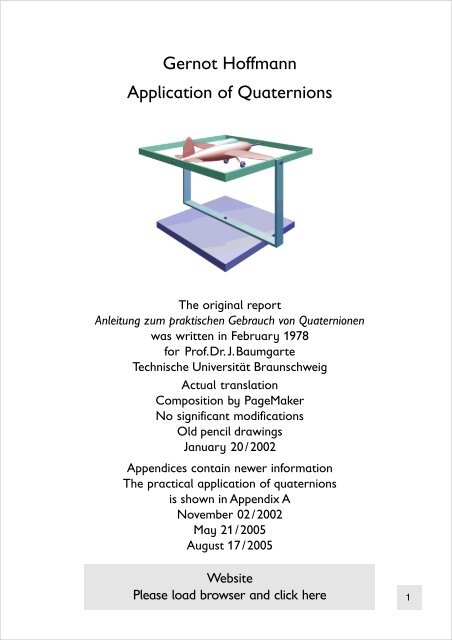
Gernot Hoffmann Application of Quaternions

Gernot Hoffmann
Application of Quaternions
The original report
Anleitung zum praktischen Gebrauch von Quaternionen
was written in February 1978
for Prof.Dr.J.Baumgarte
Technische Universität Braunschweig
Actual translation
Composition by PageMaker
No significant modifications
Old pencil drawings
January 20/2002
Appendices contain newer information
The practical application of quaternions
is shown in Appendix A
November 02/2002
May 21/2005
August 17/2005
Website
Please load browser and click here
1

Application of Quaternions
Contents
1. Definition and Features 3
2. Rotational Transformations 5
3. Transformation of Angular Velocities 7
4. Rotational Equation of Motion in Euler Formulation 11
4.1 Rotational Euler Equation by Quaternions
4.2 Transformation of Torques
5. Rotational Equation of Motion in Lagrange Formulation 14
5.1 Rotational Lagrange Equation by Quaternions
5.2 Transformation of Torques
6. Transformations for Classical Euler Angles 16
6.1 Rotational Transformations
6.2 Transformations by Quaternions
6.3 Calculation of Angles
7. Transformations for Aircraft Angles 18
7.1 Rotational Transformations
7.2 Transformations by Quaternions
7.3 Calculation of Angles
8. References 20
8.1 Original References
8.2 References quoted from [1]
9. Appendix A Rigid Body Rotation Half-Quat 21
10. Appendix B Rigid Body Rotation Full-Quat 32
11. Appendix C Spherical Linear Interpolation 37
2

1. Definition and Features
Quaternions are quadrupels of real numbers, for which a special multiplication is defined.
(1.1) Q =
The rules for the multiplication are easily understood if we represent the quaternions by three complex
base vectors i, j, k. Then we have
(1.2) Q = q 1 i + q 2 j + q 3 k +q 4 .
The first three components can be written as a vector or column matrix q :
(1.3) Q = q + q 4
This scheme is valid for the multiplication, e.g. j·k = i :
(1.4)
q 1
q 2
q 3
q 4
Now we can already execute the multiplication of two quaternions Q and S. Opposed to matrix
multiplications, we use always the dot.
(1.5) P = Q·S
(1.6) Q·S= (q 1 i + q 2 j + q 3 k + q 4 )·(s 1 i + s 2 j + s 3 k + s 4 ) = p 1 i + p 2 j + p 3 k + p 4 = p + p 4
p1 q4 - q3 q2 q1 s1 p2 q3 q4 - q1 q2 s
(1.7) =
2
p3 - q2 q1 q4 q3 s3 p4 - q1 - q2 - q3 q4 s4 The result of the multiplication is the product of the quaternion matrix R(Q) , which is assigned to Q,
and the quaternion S, written as column matrix:
(1.8) P = R(Q) S
i j k
i -1 k -j
j -k - 1 i
k j - i -1
In [3] it is shown, that the multiplication can be executed by using normal, dot and cross products:
(1.9) P = p + p 4 =(q 4 s 4 - q T s) + (q 4 s + s 4 q + q × s)
It is q T s the dot product and q × s the cross product of the vector part of the quaternions.
3

Each quaternion has a conjugate quaternion Q' :
(1.10) Q' =
- q 1
- q 2
- q 3
+ q 4
The multiplication is not commutative but associative:
(1.11) Q 1 ·Q 2 ≠ Q 2 ·Q 1
Q 1 ·Q 2 ≠ - Q 2 ·Q 1
Q 1 ·(Q 2 ·Q 3 ) = (Q 1 ·Q 2 )·Q 3
The following rule can be derived from Eq.(1.9) :
(1.12) (Q·S)'= S'·Q'
(1.13) S'·Q' = (q 4 s 4 - (-s) T (-q)) + (q 4 (-s) + s 4 (-q) + (-s)×(-q))
=(q 4 s 4 - q T s) - (q 4 s + s 4 q + q×s) =(S·Q)'
The norm of a quaternion is one or has to be made to one:
(1.14) Q·Q' = q 1 2 + q2 2 + q3 2 + q4 2 = 1
For Q = Q(t) we have
· ·
(1.15) Q·Q' + Q·Q' = 0 .
Definition and Features
William Rowan Hamilton (1805 - 1865) had invented the quaternions.
Arthur Cayley (1821 - 1895) and Felix Klein (1849 - 1925) had contributed further.
4

2. Rotational Transformations
We consider quaternions with this structure and want to execute coordinate system rotations:
(2.1) Q = cos(α/2) - n sin(α/2)
The same physical vector x has the column matrix x 1 in coordinate system 1 and x 2 in system 2.
System 2 is rotated relative to system 1 by a right screw rotation about n with the angle α .
Then we have these transformations for the column matrices:
(2.2) x 2 = Q·x 1 ·Q'
(2.3) x 1 = Q'·x 2 ·Q
We can verify this rule by an example.
Rotate by α about the axis z 1 .
Note: the rotation axis vector n has the same column matrices n 1 = n 2 in both coordinate systems.
For the special case we assign k to n and get:
(2.4) Q = cos(α/2) - k sin(α/2)
(2.5) Q' = cos(α/2) + k sin(α/2)
(2.6) x 2 = ( cos(α/2) - k sin(α/2) )·(x 1 i + y 1 j + z 1 k)·( cos(α/2) + k sin(α/2) )
x1 [ cos2 (α/2) - sin2 (α/2)] + 2y1 [ sin(α/2)cos(α/2) ]
(2.7) x2 = -2x1 [ sin(α/2)cos(α/2) ] + y1 [cos2 (α/2) - sin2 (α/2)]
cos(α) sin (α) 0
(2.8) x2 = - sin (α) cos(α) 0 x1 0 0 1
This is the well known rotation matrix for the coordinate
transformation of a fixed vector.
Note: the fourth component in the quaternion product
Q·x·Q' is always zero.
Several sequential rotations about arbitrary axes are
described by sequential quaternion products:
x 2 = Q 1 · x 1 ·Q 1 '
(2.9) x 3 = Q 2 ·x 2 ·Q 2 '
x4 = Q 3 ·x 3 ·Q 3 '
(2.10) x 4 = Q 3 ·Q 2 ·Q 1 ·x 1 ·Q 1 '·Q 2 '·Q 3 ' =
z 1
Q·x 1 ·Q'
5

Rotational Transformations
In each quaternion Q the components q1,q2,q3 and q4 depend on the type and sequence of rotation
angles, which are called Euler angles or Cardan angles.
But it is possible to express the left-right quaternion product for all cases by one matrix multiplication:
(2.11) x 4 = C 41 x 1
The so-called Cayley matrix C 41 is calculated straightforward.
q 1 2 -q2 2 -q3 2 +q4 2 2(q 1 q 2 -q 3 q 4 ) 2(q 1 q 3 +q 2 q 4 )
(2.12) C 41 = 2(q 1 q 2 +q 3 q 4 ) -q 1 2 +q2 2 -q3 2 +q4 2 2(-q 1 q 4 +q 2 q 3 )
2(q 1 q 3 -q 2 q 4 ) 2(q 1 q 4 +q 2 q 3 ) -q 1 2 -q2 2 +q3 2 +q4 2
Opposed to coordinate system rotations, a body rotation uses this equation:
(2.13) Q = cos(α/2) + n sin(α/2) .
This can be easily explained by replacing the angle by the negative angle.
The quaternion coordinate system rotation can be alternatively defined by this formulation:
(2.14) Q = cos(α/2) + n sin(α/2)
Then all transformations have to be written in this order:
( 2.15) x 2 = Q'·x 1 ·Q
The Cayley matrix has to be substituted by the transposed.
6

3. Transformation of Angular Velocities
The coordinate system 4 rotates relative to system 1 with the angular velocity ω 14 . This physical vector
is described as a column matrix ω 4 14 in system 4 . The vector, which is fixed in 1, has then a time
variable component in 4 . Euler´s formula delivers for this coordinate transformation :
·
(3.1) x 4 = -ω 4 14 × x4
Now we show by an example that the sign is correct.
·
(3.2) ω 4 12 = ( 0 , 0 , α ) T
(3.3) x 2 = ( x 2 , y 2 , 0 ) T
· · · · · ·
(3.4) x 2 = ( x 2 , y 2 , z 2 ) T = ( y 2 α , - x 2 α , 0 ) T
It can be seen in the drawing, that indeed x 2 increases
and y 2 decreases.
Now we look for a similar relation for quaternions, based on the coordinate transformation
(3.5) x 4 = Q·x 1 ·Q'.
For a constant x 1 we find the derivative
· · ·
(3.6) x 4 = Q·x 1 ·Q' + Q ·x 1 ·Q'
Because of
(3.7) x 1 = Q'·x 4 ·Q
and with Q·Q' = 1 we find
· · ·
(3.8) x 4 = Q·Q'·x 4 ·Q·Q' + Q·Q'·x 4 ·Q·Q' ,
· · ·
(3.9) x 4 = Q·Q'·x 4 + x 4 ·Q·Q' .
By differentiation of the norm
· ·
(3.10) 0 = Q·Q' + Q·Q'
we get
· · ·
(3.11) x 4 = Q·Q'·x 4 - x 4 ·Q·Q' .
Now we omit for clarity the index for the coordinate system and write simply
·
(3.12) T = Q·Q' = t + t 4 .
7

Using Eq.(1.9) we find
(3.13) T·x = t T x + t 4 x + t × x ,
(3.14) - x·T = - t T x - t 4 x - x× t ,
·
(3.15) x = 2t × x .
By comparison with Eq.(3.1) we see
(3.16) ω = - 2t .
Transformation of Angular Velocities
Now we add a fourth component and build a quaternion
(3.17) ω = ω ω + + ω4 = - 2T = - 2 Q ·Q' .
Now we use again Eq.(3.10)
· ·
(3.18) Q·Q' = - Q·Q'
and because of Eq.(1.15) we have
· ·
(3.19) (Q·Q')' = Q·Q' .
Therefore this is also valid:
· ·
(3.20) (Q·Q')' = - Q·Q'
(3.21) T = - T'
This means, that the fourth component t 4 = ω 4 /2 is always zero.
So far we have the intermediate result
· ·
(3.22) ω ω + + ω4 = - 2 Q ·Q' = 2Q·Q' ,
which should be shown as a matrix multiplication of this type:
(3.23) ω ω + + ω4 = W(Q) Q
·
· ·
In Eq.(3.22) we have 2Q·Q' , but we want to express the angular velocity in Q .
Therefore we apply the matrix multiplication Eq.(1.9) explicitely (next page).
8

(3.24)
Transformation of Angular Velocities
·
- q 1
· ·
R(Q) Q' - q2 ·
- q3 ·
q4 q4 - q3 q2 q1 · · · ·
- q4q1 +q3q2 -q2q3 +q1q4 q3 q4 - q1 q2 · · · ·
- q3q1 -q4q2 +q1q3 +q2q4 - q2 q1 q4 q3 · · · ·
q2q1 - q1q2 -q4q3 +q3q4 - q1 - q2 - q3 q4 · · · ·
q1q1 +q2q2 +q3q3 +q4q4 Then we find, using a new matrix V :
· ·
(3.25) ω = W(Q) Q = 2 V(Q) Q
(3.26) V =
- q 4 q 3 - q 2 q 1
- q 3 - q 4 q 1 q 2
q 2 - q 1 - q 4 q 3
q 1 q 2 q 3 q 4
V T =
·
Because of ω4 = 2 Σ qiqi = d/dt Q·Q' we find ω4 = 0.
It can be easily shown for normalized quaternions: V V T = I .
V is orthogonal (orthonormal) and we have furtheron
(3.27) V -1 = V T ,
(3.28) W -1 = (1/2)V T = (1/4)W T .
The inverse exists for all q i .
- q 4 - q 3 q 2 q 1
q 3 - q 4 - q 1 q 2
- q 2 q 1 - q 4 q 3
q 1 q 2 q 3 q 4
Note:
Somewhere one may find V(Q) replaced by V T (Q) . This is a result of a different definition of the
quaternion coordinate rotation by Eq.(2.14) .
This should not be confused with body rotations. In our preferred formulation, a body rotation looks
also like Eq.(2.14), but in fact it is the conjugate of Eq.(2.1)
(3.29) Q = cos(α/2) + n sin(α/2) .
9

Transformation of Angular Velocities
An example shows that Eq.(3.25) is correct. Again we rotate by α about the z-axis.
(3.30) Q = cos(α/2) - k sin(α/2) = =
0
0
- sin (α/2)
q4 cos(α/2)
- cos(α/2) - sin(α/2) 0 0 0
(3.31) ω = 2
sin (α/2)
0
0
- cos(α/2)
0
0
0
- cos(α/2)
- sin(α/2)
0
- sin(α/2)
cos(α/2)
0
·
- (α/2) cos(α/2)
·
- (α/2) sin (α/2)
(3.32) ω = ( 0 , 0 , α , 0 ) T
·
Further features of the matrix V (we write the quaternion as a transposed column):
(3.33) V(Q)Q = ( 0 , 0 , 0, 1 ) T
· ·
(3.34) 0 = V Q + V Q
· ·
(3.35) V Q= - V Q
q1 q2 q3 · · · ·
(3.36) V(Q)Q = V(Q) Q = V(P) P = ( 0 , 0 , 0, 1) T
10

4. Rotational Equation of Motion in Euler Formulation
4.1 Rotational Euler Equations by Quaternions
We consider the rotation of a rigid body with the body fixed coordinate system x B = x 4 relative to an
inertial system x I = x 1 . Now we need an observer system x o in which all physical vectors are written as
column matrices. The lower index indicates always the observer system.
The Euler formulation for the angular momentum in rotating observer coordinates:
·
(4.1) L IB
o + ωoIO × LoIB = MoB ω IB Vector of the angular velocity of the body relative to the inertial system,
ω IO Vector of the angular velocity of the observer relative to the inertial system
L IB Angular momentum
J Tensor of inertia (a 3x3 matrix)
M B Torque
(4.2) L IB = J ω IB
In most cases the observer system is either the inertial system or it is body fixed. We use the body fixed
system and replace therefore in all equations o by B .
This is especially useful to avoid a time variable tensor of inertia. Furtheron, many torques can be
expressed easier in body fixed coordinates, e.g. for an aircraft.
·
(4.3) L IB
B + ωBIB ×LBIB = MBB In the next step we extend all column matrices to four dimensions, though this has mostly no physical
meaning. We write the new elements not bold.
L IB
B ω ω IO
B M B
B
(4.4) L = ω = M =
L 4 ω 4 M 4
J B 0
(4.5) J = with J 4 > 0
0 T J 4
Cross products are written as matrix products, e.g. for N = ω ω × L in the new nomenclature:
(4.6) N = ω × L ⇒ N = Ω L
0 - ω z ω y
ω z 0 - ω x 0
(4.7) Ω = - ω y ω x 0
(4.8) N =
ω y L z - ω z L y
ω z L x - ω x L z
ω x L y - ω y L x
0 4 L 4
0 T 0 4
Because of ω 4 = 0 in Eq.(3.21) we have L 4 = 0, therefore I 4 and 0 4 are so far not relevant.
11

Rotational Equation of Motion in Euler Formulation
With Eq.(3.25) the equation for the angular momentum, Eq.(4.3), is already in quaternion formulation:
(4.9) 2 d/dt (JVQ) + 2 ΩJ VQ = M(Q,Q,t)
(4.10) JVQ + JVQ + ΩJVQ = (1/2) M(Q,Q,t)
According to Eq.(3.36) the term VQ is zero. The inertia term (JV) is never singular, if the extended
tensor of inertia is positive definite. Especially no moment of inertia on the main diagonal should be
zero. V itself is orthogonal, therefore all inverse operators exist:
(4.11) ( J V) -1 =V -1 J -1 = V T J -1
Multiplying the equation from the left side results in
(4.12) Q + V T J -1 ΩJ VQ = (1/2) V T J -1 M .
Later it will be shown that Ω can be expressed by
(4.13) Ω =2VV T = 2V V T (Q) ,
and we do not need the less elegant conversion ω ⇒ Ω.
Now we write the differential equation as a first order system:
(4.14) Q = P
(4.15) P = - 2 V T J -1 V V T (P)JVP + (1/2)V T J -1 M(Q,P,t)
As long as Ω is not substituted we use
(4.16) ω = 2VP
· ·
· · ·· · ·
·· ·
·
·
· ·
for building Ω in each step of a numerical solution.
The reverse transformation from quaternions to physical angles is here not yet possible, because this
depends on the specific sequence of Euler or Cardan angles (chapters 6 and 7).
A physical torque can be applied as a general function M(Q,P,t) in body fixed coordinates, in inertial
coordinates or in a mechanical gimbal system in gimbal coordinates. Finally we need the torque in body
fixed coordinates.
(4.17) M B = S BA (Q) M A (Q,P,t)
· ·
4.2 Transformation of Torques
·
In this formulation, S BA (Q) is a placeholder for the transformation from an arbitrary source coordinate
system, where the torque can be easily described. A=B is the body fixed system, A=1=I is the inertial
system. A=3 is the last gimbal of three .
12

Rotational Equation of Motion in Euler Formulation
For the moment, we refer to a physical torque M = M(ω,α,α,t). Is it possible under all circumstances to
replace the physical variables by quaternions ?
The angles can be replaced if we use a specific set of Euler or Cardan Angles., e.g. Eq.(6.18).
The angular velocity is easily replaced by
(4.18) ω = 2V(Q)Q .
Again we refer to physical variables, e.g. Eq.(6.16):
(4.19) ω = B(α) α
α
The matrix B becomes singular in one orientation, for the classical Euler angles for θ=0.
It´s well known, that a set of physical angles can cause the so called gimbal lock.
Then Eq.(4.19) cannot be inverted:
·
(4.20) α = B -1 ω
Is it possible to cure the problem by quaternions ?
The figure shows a free-running gyro in gimbals. For example, we have some friction in gimbal bearings,
·
which may be modelled by a function M(α). Therefore we have to calculate these torques by explicite
·
use of α α . Quaternions don´t cure the problem for systems with mechanical gimbals.
In the gimbal lock orientation θ= 0 we find by use of Eq.(6.16):
ωx 0 cos(ψ) 0 φ
·
(4.21) ωy = 0 - sin (ψ) 0 θ
·
ωz 1 0 1 ψ
·
·
It is not possible to express ω z uniquely by φ and ψ .
·
· ·
For the gyro in gimbals, the problem can be solved by equations of motions for the flywheel and all
gimbals as well. Instead three differential equations of second order we have then nine equations.
This gyro is of course not a reasonable practical design. E.g. for an artificial horizon one would not use
the classical Euler angles, but Cardan angles, where the gimbals are orthogonal in normal
position. Then, an aircraft would have gimbal lock in a vertical climb.
13
·

5. Rotational Equation of Motion in Lagrange Formulation
5.1 Rotational Lagrange Equation by Quaternions
The rotational part of the kinetic energy is a quadratic form:
(5.1) T = (1/2)ω T J ω
The angular velocity is ω= ω IB and the tensor of inertia J is constant in body fixed coordinates.
Using Eq.(3.25) and Eq.(3.35) the energy can be expressed in quaternions:
(5.2) T = 2 Q T V T JVQ
(5.3) T = 2 Q T V T JVQ
Lagrange equations:
d ∂ T ∂ T
(5.7) –– ––– · – ––– = ML dt ∂Q ∂Q
The physical meaning of M L is not yet clear. If Q is a set of generalized coordinates then M L should be
the generalized torque. A quadratic form is derived like this:
(5.5) –– xT d
Ax = 2 Ax
dx
Now we derive the parts of the Lagrange equation:
∂ T
·
∂Q
d ∂ T
·
dt ∂Q
∂ T
∂Q
· ·
(5.6) ––– = 4VTJVQ = 2 VT ·
Jω
(5.7) –– ––– = 2V T Jω + 2V T Jω
(5.8) ––– = 4VTJV Q = - 2VT · · ·
Jω
Assembled, and using VQ = 0 for the first three components:
(5.9) 2V T Jω + 2V T Jω + 2V T Jω = M L
(5.10) ω = 2VQ + 2VQ
· ·
· · ·
· · · · ·
(5.11) 4V T JVQ + 8V T JVQ = M L
· ·
· ·
· ·
· · · ·
· ·
(5.12) JVQ + 2VV T JVQ = (1/4) VM L
The Lagrange Equation can be written as as a first order system. The inverse of the tensor of inertia
exists.
14

Rotational Equation of Motion in Lagrange Formulation
Now we write the differential equation as a first order system:
(5.13) Q = P
·
·
(5.14) P = - 2V T J -1 VV T JVP + (1/4) V T J -1 VM L
The reverse transformation from quaternions to physical angles is here not yet possible, because it
depends on the specific sequence of Euler or Cardan angles (chapters 6 and 7).
5.1 Transformation of Torques
Eq.(5.12) is the same as Eq.(4.10). By comparison we find:
(5.15) Ω = 2VV T
(5.16) M = (1/2)VM L
The last equation shows the relation between the body fixed torque M and the torque in the Lagrange
equation M L .
(5.17) M L = 2V T M
This is, ignoring the factor 4, equivalent to the transformation of angular velocities:
·
·
(5.18) Q = (1/2)V Tω
·
·
15

6. Transformations for Classical Euler Angles
6.1 Rotational Transformations
Rotation about z 1 with φ :
(6.1) x 2 = T 21 x 1
cos(φ) sin (φ) 0
(6.2) T 21 = - sin(φ) cos(φ) 0
0 0 1
(6.3) Q 1 = cos(φ/2) - k sin(φ/2)
Rotation about x 2 with θ :
(6.4) x 3 = T 32 x 2
1 0 0
(6.5) T 32 = 0 cos(θ) sin (θ)
0 - sin (θ) cos(θ)
(6.6) Q 2 = cos(θ/2) - i sin(θ/2)
Rotation about z 3 with ψ :
(6.7) x 4 = T 43 x 3
cos(ψ) sin (ψ) 0
(6.8) T 43 = - sin(ψ) cos(ψ) 0
0 0 1
(6.9) Q 3 = cos(ψ/2) - k sin(ψ/2)
Three angle rotation:
(6.10) x 4 = T 41 x 1
(6.11) T 41 = T 43 T 32 T 21
cos(ψ) sin (ψ) cos(θ) sin (ψ) sin (θ)
(6.12) T 42 = - sin(ψ) - cos(ψ) sin (θ) cos(ψ) sin (θ)
0 - sin (θ) cos(θ)
cos(ψ) cos(φ) cos(ψ) sin (φ) sin(ψ) sin (θ)
(6.13) T41 =
- sin (ψ) cos(θ) sin (φ) + sin (ψ) cos(θ) cos(φ)
- sin(ψ) cos(φ) - sin (ψ) sin (φ)
- cos(ψ) cos(θ) sin (φ) + cos(ψ) cos(θ) cos(φ)
cos(ψ) sin (θ)
sin (θ) sin (φ) - sin (θ) cos(φ) cos(θ)
Reverse transformation:
(6.14) x 1 = T 41 -1 x4 = T 41 T x4
16

6.2 Transformation of Angular Velocities
The angular velocities about Euler axes must be transformed by appropriate rotation matrices into the
body fixed system.
0 θ 0
(6.15) ω 14
4 = T43T32 0 + T
· 43
φ
0 + 0
·
0 ψ
sin (θ) sin (ψ) cos(ψ) 0 φ
(6.16) ω 14
·
4 = sin (θ) cos(ψ) - sin(ψ) 0 θ
·
cos(θ) 0 1 ψ
(6.17) ω 4 14 = B (φ, θ, ψ) T = B α
A singularity happens for Det(B) = - sin(θ) = 0 , especially for θ = 0° .
q1 0
(6.18)
q2 0
= Q
q3 3 ·Q2 ·Q1 = R(Q3 ) R(Q2 )Q1 - sin (φ/2)
q4 cos(φ/2)
cos(θ/2) 0 0 - sin(θ/2) - sin(θ/2) cos(φ/2)
0 cos(θ/2) sin(θ/2) 0 - sin(θ/2) sin (φ/2)
0 - sin(θ/2) cos(θ/2) 0 - cos(θ/2) sin (φ/2)
sin(θ/2) 0 0 cos(θ/2) cos(θ/2) cos(φ/2)
cos(ψ/2) sin (ψ/2) 0 0 - cos(ψ/2) sin(θ/2) cos(φ/2) - sin (ψ/2) sin(θ/2) sin (φ/2)
- sin (ψ/2) cos(ψ/2) 0 0 sin (ψ/2) sin (θ/2) cos(φ/2) - cos(ψ/2) sin(θ/2) sin (φ/2)
0 0 cos(ψ/2) -sin (ψ/2) - cos(ψ/2) cos(θ/2) sin (φ/2) - sin (ψ/2) cos(θ/2) cos(φ/2)
0 0 sin (ψ/2) cos(ψ/2) sin (ψ/2) cos(θ/2) sin (φ/2) +cos(ψ/2) cos(θ/2) cos(φ/2)
The Euler angles for a quaternion are found by comparing the Cayley matrix Eq.(2.12) and the Euler
matrix Eq. (6.13).
(6.19) x 4 = T 41 x 1 = C 41 x 1
(6.20) c 13 = sin(ψ)sin(θ)
c 23 = cos(ψ)sin (θ)
c 31 = sin(θ) sin (φ)
c 32 = - sin (θ) cos(φ)
c 33 = cos(θ)
(6.21) tan(ψ) = c 13 /c 23
tan(φ) = -c 31 /c 32
tan(θ) = sqrt(c 13 2 + c23 2 )/c33
Transformations for Classical Euler Angles
· · · ·
6.3 Transformations by Quaternions
6.4 Calculation of Angles
·
A four quadrant function z(y,x) = arctan(y/x) is necessary. Singularity 0/0 for θ = 0 .
·
17

Rotation about z 1 with ψ :
(7.1) x 2 = T 21 x 1
7. Transformations for Aircraft Angles
7.1 Rotational Transformations
cos(ψ) sin (ψ) 0
(7.2) T 21 = - sin(ψ) cos(ψ) 0
0 0 1
(7.3) Q 1 = cos(φ/2) - k sin(φ/2)
Rotation about y 2 with θ :
(7.4) x 3 = T 32 x 2
cos(θ) 0 - sin(θ)
(7.5) T 32 = 0 1 0
sin (θ) 0 cos(θ)
(7.6) Q 2 = cos(θ/2) - j sin(θ/2)
Rotation about x 3 with φ :
(7.7) x 4 = T 43 x 3
1 0 0
(7.8) T43 = 0
0
cos(φ)
- sin (φ)
sin (φ)
cos(φ)
(7.9) Q 3 = cos(ψ/2) - i sin(ψ/2)
Three angle rotation:
(7.10) x 4 = T 41 x 1
(7.11) T 41 = T 43 T 32 T 21
cos(θ) 0 - sin(θ)
(7.12) T 42 = sin (θ) sin (φ) cos(φ) cos(θ) sin (φ)
sin (θ) cos(φ) - sin (φ) cos(θ) cos(φ)
(7.13) T 41 =
Reverse transformation:
(7.14) x 1 = T 41 -1 x4 = T 41 T x4
cos(ψ) cos(θ) sin (ψ)cos(θ) - sin (θ)
- sin (ψ) cos(φ) cos(ψ) cos(φ) cos(θ) sin (φ)
+cos(ψ) sin (θ) sin (φ) + sin (ψ) sin (θ) sin (φ)
sin (ψ) sin (φ) - cos(ψ) sin (φ) cos(θ) cos(φ)
cos(ψ) sin (θ) cos(φ) + sin (ψ) sin (θ) cos(φ)
18

7.2 Transformation of Angular Velocities
The angular velocities about Euler axes must be transformed by appropriate rotation matrices into the
body fixed system.
0 0 φ
(7.15) ω 14
·
4 = T43T32 0 + T43 θ + 0
·
ψ 0 0
- sin (θ) 0 1 ψ
(7.16) ω 14
·
4 = sin (φ) cos(θ) cos(φ) 0 θ
·
cos(φ) cos(θ) - sin(φ) 1 φ
(7.17) ω 4 14 = B (ψ,θ, φ) T = B α
A singularity happens for Det(B) = - cos(θ) = 0 , especially for θ = 90° .
q1 0
(7.18)
q2 0
= Q
q3 3 ·Q2 ·Q1 = R(Q3 ) R(Q2 )Q1 - sin (ψ/2)
q4 cos(ψ/2)
cos(θ/2) 0 - sin(θ/2) 0 sin (ψ/2) sin (θ/2)
0 cos(θ/2) 0 - sin(θ/2) - cos(ψ/2) sin (θ/2)
sin(θ/2) 0 cos(θ/2) 0 - sin (ψ/2) cos(θ/2)
0 sin(θ/2) 0 cos(θ/2) cos(ψ/2) cos(θ/2)
cos(φ/2) 0 0 - sin (φ/2) sin (ψ/2) sin (θ/2) cos(φ/2) - cos(ψ/2) cos(θ/2) sin (φ/2)
0 cos(φ/2) sin (φ/2) 0 - cos(ψ/2) sin (θ/2) cos(φ/2) - sin (ψ/2) cos(θ/2) sin (φ/2)
0 - sin (φ/2) cos(φ/2) 0 cos(ψ/2) sin (θ/2) sin (φ/2) - sin (ψ/2) cos(θ/2) cos(φ/2)
sin (φ/2) 0 0 cos(φ/2) sin (ψ/2) sin(θ/2) sin (φ/2) +cos(ψ/2) cos(θ/2) cos(φ/2)
The Euler angles for a quaternion are found by comparing the Cayley matrix Eq.(2.12) and the Euler
matrix Eq. (7.13).
(7.19) x 4 = T 41 x 1 = C 41 x 1
(7.20) c 11 = cos(ψ) cos(θ)
c 12 = sin(ψ)cos(θ)
c 13 = -sin (θ)
c 23 = cos(θ) sin (φ)
c 33 = cos(θ) cos(φ)
(7.21) tan(ψ) = c 12 /c 11
tan(φ) = c 23 /c 33
tan(θ) =-c 13 / sqrt(c 11 2 + c12 2 )
Transformations for Aircraft Angles
· · · ·
7.3 Transformations by Quaternions
7.4 Calculation of Angles
A four quadrant function z(y,x) = arctan(y/x) is necessary. Singularity 0/0 for θ = 90° .
·
·
19

8.1 Original References
8. References
[1] Steuer, A. Die Beschreibung räumlicher Bewegungen durch Quaternionen
Seminarvortrag am Lehrstuhl für Flugmechanik
TU Braunschweig, 1972
[2] Lohe, R. Die Beschreibung der Bewegungsgleichungen des Kreisels
Seminarvortrag am Lehrstuhl A für Mechanik
TU Braunschweig, 1976
[3] Corben, H.C. Classical Mechanics
Stehle, P. John Wiley & Sons, Inc.
New York, 1957
[4] Vitins, M. Contributions to the descriptions of gyros by quaternions.
By courtesy of Prof.Dr.J.Baumgarte
[5] Wells, D.A. Lagrangian Dynamics
Schaum´s Outline Series
McGraw-Hill Book Company
New York, 1967
8.2 Some references quoted from [1]
[6] Hamel, G. Theoretische Mechanik
[7] Madelung, E. Die mathematischen Hilfsmittel des Physikers
[8] Kowalewski, G. Lehrbuch der höheren Mathematik
[9] Niemz, W. Anwendung der Quaternionen auf die allgemeinen Bewegungsgleichungen der
Flugmechanik . ZFW 11, 1963, S.368-372
[10] Goldstein, H. Klassische Mechanik
[11] Whittaker, E.T. Treatise on the Analytical Dynamics of Particles and Rigid Bodies
[12] Whittaker, E.T Analytical Dynamics
[13] Surber, T.E. On the use of quaternions to describe the angular orientation of space vehicles
J.Aerospace Sci. 28, 1961
[14] Robinson A.C. On the use of quaternions in simulation of rigid body motion
WADC TR 58-17, 1958
[15] Blaschke, W. Analytische Geometrie
[16] Sommerfeld,A. Theorie des Kreisels
Klein, F.
20

9.1 Appendix A Rigid Body Rotation Half-Quat
This chapter describes the simulation of a
rigid body rotation. The tensor of inertia is
always symmetric, but products of inertia are
not necessarily zero.
The first differential equation delivers the angular
acceleration as a function of angular
velocities and body fixed torques T.
This part is totally independent of Euler
angles, as long as the torques are not
expressed as functions of angles.
The second differential equation delivers the
quaternion derivative as a function of the angular
velocity. Because the angular velocities
are still used, the method is called Half-Quat.
The quaternion representation doesn´t suffer
from gimbal lock.
The physical interface which delivers the
Euler angles has of course a singularity at
cos(θ)=0. A simulation without gimbal lock
requires also a graphics program based on
quaternions (page 25).
·
ω = J -1 (-( ω×J ω) + T )
·
Q = (1/2) V T (Q)ω, ω 4 =0
The integration is performed by ’False Euler’.
This means that the results of the angular
velocities are immediately used as inputs for
the integration of the quaternion. Standard
Euler would use only old values on the right
side.
The quaternion norm is stabilized by a norm
controller. This algorithm is independent of
the stepsize dT. The whole system is stable
for small dT≤ 0.3 .
For vanishing products of inertia the tensor
is diagonal, and the set of equations can be
simplified.
·
ω x = (ω y ω z (J y -J z )+T x )/J x
·
ω y = (ω z ω x (J z -J x )+T y )/J y
·
ω z = (ω x ω y (J x -J y )+T z )/J z
·
Q = (1/2) V T (Q)ω
This case is not treated in the code example.
Standard aircraft angles: ψ=15°, θ =30°, φ =15°
Gimbal lock orientation: ψ= 0°, θ =90°, φ =0°
21

9.2 Appendix A Half-Quat with Euler Interface
Procedure MatObj3Da;
{ Transposed A41 for object rotation
Calculate all Sines/Cosines and the rotation matrix }
Begin
SicCoc(Ps1,sPs1,cPs1);
SicCoc(Th1,sTh1,cTh1);
SicCoc(Ph1,sPh1,cPh1);
o11:= cTh1*cPs1; o12:=-cPh1*sPs1+sPh1*sTh1*cPs1; o13:= sPh1*sPs1+cPh1*sTh1*cPs1;
o21:= cTh1*sPs1; o22:= cPh1*cPs1+sPh1*sTh1*sPs1; o23:=-sPh1*cPs1+cPh1*sTh1*sPs1;
o31:=-sTh1; o32:= sPh1*cTh1; o33:= cPh1*cTh1;
End;
Procedure Initial;
{ Initial conditions }
Begin
T:=0;
Txc:=0; Tyc:=0; Tzc:=0; { Command torques }
Psc:=0; Thc:=0; Phc:=0; { Command Angles }
W.x:=0; W.y:=0; W.z:=0; { Angular velocity }
Ps1:=0; Th1:=0; Ph1:=0; { Angles in radian }
MatObj3Da;
SicCoc(0.5*Ps1,sPs1,cPs1);
SicCoc(0.5*Th1,sTh1,cTh1);
SicCoc(0.5*Ph1,sPh1,cPh1);
{ Page 19 }
With Q Do
Begin
q1:=+sPs1*sTh1*cPh1-cPs1*cTh1*sPh1;
q2:=-cPs1*sTh1*cPh1-sPs1*cTh1*sPh1;
q3:=+cPs1*sTh1*sPh1-sPs1*cTh1*cPh1;
q4:=+sPs1*sTh1*sPh1+cPs1*cTh1*cPh1;
End;
{ P = 0.5*V’(Q)*W , not necessary for Half-Quat }
With P Do { P.p1 }
With Q Do { Q.q1 }
With W Do { W.x }
Begin
p1:=0.5*(-q4*x-q3*y+q2*z);
p2:=0.5*(+q3*x-q4*y-q1*z);
p3:=0.5*(-q2*x+q1*y-q4*z);
p4:=0.5*(+q1*x+q2*y+q3*z);
End;
SicCoc(Psc,sPsc,cPsc);
SicCoc(Thc,sThc,cThc);
SicCoc(Phc,sPhc,cPhc);
End;
Procedure Integ;
{ G.Hoffmann
ZFlug702 Half-Quat
Rotational differential equations for a rigid body
Simple angle controllers
Angular accelerations are calculated by physical variables
Angles are calculated by Quaternions
Complete tensor of inertia }
Var qn,s1,s2,s3,s4 : Double;
c11,c12,c13,c23,c33: Double;
Const Jxx=0.6; Jxy=0;
Jyy=1; Jxz=0.2;
Jzz=1.5; Jyz=0;
dampP=2; conPhi= 6;
dampQ=4; conThe=10;
dampR=5; conPsi=12;
dT =0.1;
dT2=0.5*dT;
22

9.3 Appendix A Half-Quat with Euler Interface
Begin
{ Initialization: by Initial
Installed:
Roll,Pitch,Yaw damper
Roll,Pitch Yaw angle controller by sines and cosines
Phc = Command Roll angle Txc = Command Torque
Thc = Command Pitch angle Tyc = Command Torque
Psc = Command Yaw angle Tzc = Command Torque }
If T=0 then
Begin
{ Jxx -Jxy -Jxz
-Jxy Jyy -Jyz
-Jxz; -Jyz Jzz }
FillJ33(Jxx,Jyy,Jzz,Jxy,Jxz,Jyz,J33); { Tensor of inertia }
HoInvers(3,J33,I33,c11,flag); { Inverse Tensor }
End;
T:=T+dt;
T1.x:=Txc;
T1.y:=Tyc;
T1.z:=Tzc;
If DCon Then { Dampers }
With W Do
Begin
T1.x:=T1.x-dampP*x; { Roll damper torque }
T1.y:=T1.y-dampQ*y; { Pitch damper }
T1.z:=T1.z-dampR*z; { Yaw damper }
End;
If RCon Then
T1.x:=T1.x-conPhi*(sPh1*cPhc-cPh1*sPhc); { Roll angle torque }
If Pcon Then
T1.y:=T1.y-conThe*(sTh1*cThc-cTh1*sThc); { Pitch angle }
If YCon Then
T1.z:=T1.z-conPsi*(sPs1*cPsc-cPs1*sPsc); { Yaw angle }
{ Body fixed coordinate system in arbitrary axes direction }
{ Integration for angular velocities, using old values W }
{ d/dt W = I33*(-(W x J33*W) + T1 )
d/dt W = I33*(-(W x T2 ) + T1 )
d/dt W = I33*( -TN + T1 )
d/dt W = I33*( T1 ) }
MatVec (J33,W,T2);
AcrosB (W ,T2,TN);
With T1 Do
Begin
x:=-TN.x + x;
y:=-TN.y + y;
z:=-TN.z + z;
End;
MatVec (I33,T1,TN);
With W Do
Begin
x:=x + dT*TN.x;
y:=y + dT*TN.y;
z:=z + dT*TN.z;
End;
{ Integration dQ/dt=0.5*V’(Q)*W, using new values W }
With Q Do
With W Do
Begin
q1:=q1 + dT2*(-q4*x-q3*y+q2*z);
q2:=q2 + dT2*(+q3*x-q4*y-q1*z);
q3:=q3 + dT2*(-q2*x+q1*y-q4*z);
q4:=q4 + dT2*(+q1*x+q2*y+q3*z);
End;
Two equivalent codes
With Q Do
With P do
Begin
q1:=q1+p1;
q2:=q2+p2;
q3:=q3+p3;
q4:=q4+p4;
End;
Q.q1:=Q.q1+P.p1;
Q.q2:=Q.q2+P.p2;
Q.q3:=Q.q3+P.p3;
Q.q4:=Q.q4+P.p4;
23

9.4 Appendix A Half-Quat with Euler Interface
{ Normalization controller }
With Q Do
Begin
qn:=1-Sqrt(Sqr(q1)+Sqr(q2)+Sqr(q3)+Sqr(q4));
q1:=q1 + q1*qn;
q2:=q2 + q2*qn;
q3:=q3 + q3*qn;
q4:=q4 + q4*qn;
End;
{ Check Normalization }
With Q Do
Begin
s1:=Sqr(q1); s2:=Sqr(q2); s3:=Sqr(q3); s4:=Sqr(q4);
qn:=Sqrt(s1+s2+s3+s4);
WrNumWin(2,grel,2,’qn’,qn);
End;
{ Angles by Caley matrix }
With Q Do
Begin
c11:=s1-s2-s3+s4; c12:=2*(+q1*q2-q3*q4); c13:=2*(+q1*q3+q2*q4);
c23:=2*(-q1*q4+q2*q3);
c33:= -s1-s2+s3+s4;
Ps1:=atan2( c12,c11);
Ph1:=atan2( c23,c33);
Th1:=atan2(-c13,Sqrt(Sqr(c11)+Sqr(c12)));
End;
MatObj3Da; { Elements oik, for object rotation Mode A=1 }
End;
24

9.5 Appendix A Half-Quat with Quat Interface
So far the interface to the graphics program was based on Euler angles. In the procedure MatObj3Da
the elements o ik are calculated by sines and cosines of the three angles.
We can easily replace the matrix directly by the Cayley matrix. This is done in MatObj3Qa . For clarity,
the necessary transposing is explicitely written down.
Thus, the gimbal lock problem seems to be solved. Even in a position cos(θ)=0 we can apply a torque
about the body fixed z-axis and the body rotates really about this axis (additionally we have in the
example some cross coupling because of J xz =0.2). This would look quite wrong if we showed the
gimbals mechanically (page 21). But it´s correct - the aircraft doesn´t have gimbals.
Did we really get rid of the gimbal lock problem ?
No - as long as the angle controller is based on Euler angles, this control system cannot be used in the
vicinity of singularity orientations.
Now we have three alternatives:
1. Operate the controller only for limited angles (as in the example, though not explicitely restricted).
2. Establish a second set of Euler angles and toggle between both.
3. Define the control system by quaternions.
The last alternative is described in chapter 9.8. It is still necessary to define physical command angles
and therefore the connection to measuring equipment is difficult.
25

9.6 Appendix A Half-Quat with Quat Interface
Procedure MatObj3Qa;
Var s1,s2,s3,s4 : Double;
c11,c12,c13 : Double;
c21,c22,c23 : Double;
c31,c32,c33 : Double;
Begin
With Q Do
Begin
s1:=Sqr(q1); s2:=Sqr(q2); s3:=Sqr(q3); s4:=Sqr(q4);
c11:= s1-s2-s3+s4; c12:=2*(+q1*q2-q3*q4); c13:=2*(+q1*q3+q2*q4);
c21:=2*(+q1*q2+q3*q4); c22:= -s1+s2-s3+s4; c23:=2*(-q1*q4+q2*q3);
c31:=2*(+q1*q3-q2*q4); c32:=2*(+q1*q4+q2*q3); c33:= -s1-s2+s3+s4;
{ Calculate physical variables for the controller }
Ps1:=atan2( c12,c11);
Ph1:=atan2( c23,c33);
Th1:=atan2(-c13,Sqrt(Sqr(c11)+Sqr(c12)));
SicCoc(Ps1,sPs1,cPs1);
SicCoc(Th1,sTh1,cTh1);
SicCoc(Ph1,sPh1,cPh1);
End;
{ Replace elements oik in rotation matrix MatObj3Da }
o11:=c11; o12:=c21; o13:=c31;
o21:=c12; o22:=c22; o23:=c32;
o31:=c13; o32:=c23; o33:=c33;
End;
Procedure Integ;
{ G.Hoffmann
ZFlug802 Half-Quat using quaternions for graphics too
Rotational differential equations for a rigid body
Simple angle controllers
Angular accelerations are calculated by physical variables
Angles are calculated by quaternions
Complete tensor of inertia }
Var qn,det: Double;
Const Jxx=0.6; Jxy=0;
Jyy=1; Jxz=0.2;
Jzz=1.5; Jyz=0;
dampP=2; conPhi= 6;
dampQ=4; conThe=10;
dampR=5; conPsi=12;
dT =0.1;
dT2=0.5*dT;
Begin
{ Initialization: by Initial, previous chapter, using MatObj3Qa
Installed:
Roll,Pitch,Yaw damper
Roll,Pitch Yaw angle controller by sines and cosines
Phc = Command Roll angle Txc = Command Torque
Thc = Command Pitch angle Tyc = Command Torque
Psc = Command Yaw angle Tzc = Command Torque }
If T=0 then
Begin
{ Jxx -Jxy -Jxz Jxx = Integral (y*y+z*z)*dm
-Jxy Jyy -Jyz Jxy = Integral x*y*dm etc.
-Jxz; -Jyz Jzz }
FillJ33(Jxx,Jyy,Jzz,Jxy,Jxz,Jyz,J33); { Tensor of inertia }
HoInvers(3,J33,I33,det,flag); { Inverse Tensor }
End;
T:=T+dt;
T1.x:=Txc;
T1.y:=Tyc;
T1.z:=Tzc;
26

9.7 Appendix A Half-Quat with Quat Interface
If DCon Then { Dampers }
With W Do
Begin
T1.x:=T1.x-dampP*x; { Roll damper torque }
T1.y:=T1.y-dampQ*y; { Pitch damper }
T1.z:=T1.z-dampR*z; { Yaw damper }
End;
If RCon Then
T1.x:=T1.x-conPhi*(sPh1*cPhc-cPh1*sPhc); { Roll angle torque }
If Pcon Then
T1.y:=T1.y-conThe*(sTh1*cThc-cTh1*sThc); { Pitch angle }
If YCon Then
T1.z:=T1.z-conPsi*(sPs1*cPsc-cPs1*sPsc); { Yaw angle }
{ Body fixed coordinate system in arbitrary axes direction }
{ Integration for angular velocities, using old values W }
{ d/dt W = I33*(-(W x J33*W ) + T1 )
d/dt W = I33*(-(W x T2 ) + T1 )
d/dt W = I33*( -TN + T1 )
d/dt W = I33*( T1 ) }
MatVec (J33,W,T2);
AcrosB (W ,T2,TN);
With T1 Do
Begin
x:=-TN.x + x;
y:=-TN.y + y;
z:=-TN.z + z;
End;
MatVec (I33,T1,TN);
With W Do
Begin
x:=x + dT*TN.x;
y:=y + dT*TN.y;
z:=z + dT*TN.z;
End;
{ Integration dQ/dt=0.5*V’(Q)*W, using new values W }
With Q Do
With W Do
Begin
q1:=q1 + dT2*(-q4*x-q3*y+q2*z);
q2:=q2 + dT2*(+q3*x-q4*y-q1*z);
q3:=q3 + dT2*(-q2*x+q1*y-q4*z);
q4:=q4 + dT2*(+q1*x+q2*y+q3*z);
End;
{ Normalization controller }
With Q Do
Begin
qn:=1-Sqrt(Sqr(q1)+Sqr(q2)+Sqr(q3)+Sqr(q4));
q1:=q1 + q1*qn;
q2:=q2 + q2*qn;
q3:=q3 + q3*qn;
q4:=q4 + q4*qn;
End;
{ Check Normalization }
With Q Do
Begin
qn:=Sqrt(Sqr(q1)+Sqr(q2)+Sqr(q3)+Sqr(q4));
WrNumWin(2,grel,2,’qn’,qn);
End;
{ Angles by Caley matrix }
MatObj3Qa;
End;
27

9.8 Appendix A Half-Quat with Quat Controller
In this chapter we try to install an angle control system which is fully based on quaternions. Any physical
command angle is allowed.
In gimbal lock orientation the roll angle and the yaw angle are truly additive. Then the simulated gimbals
show nonsensical movements (gimbal flip) and the indicated angle values look nonsensical as well.
This doesn´t matter because the aircraft doesn´t have gimbals and the decoding of angles by use of the
Cayley matrix is still singular, it´s simply an unnecessary information.
The command angles are expressed as a quaternion Q c by the procedure AngToQuat. The deviations
dQ = Q c -Q and dR= -Q c -Q are calculated. The version with the smaller Euclidian norm is taken and
converted into body fixed torques. Q c and - Q c mean the same command position but the the selection
guarantees the shortest path under all circumstances.
As a practical result, the aircraft can be brought back from any orientation to zero angle position on a
short path. This short path reminds to the interpolation by quaternions.
The torques are optionally limited for two purposes: to match technical constraints and to check whether
the quaternion norm controller would fail because of nonsymmetrical torques or different quaternion
velocities.
Altogether this system works quite good. Not optimized damping was chosen on purpose, therefore an
overshoot is always visible.
28

9.9 Appendix A Half-Quat with Quat Controller
Procedure MatObj3Qa;
{ In previous chapter }
Procedure AngToQuat (Psi,The,Phi: Double; Var Q: QType);
Var sPsi,cPsi,sThe,cThe,sPhi,cPhi: Double;
Begin
SicCoc(0.5*Psi,sPsi,cPsi);
SicCoc(0.5*The,sThe,cThe);
SicCoc(0.5*Phi,sPhi,cPhi);
With Q Do
Begin
q1:=+sPsi*sThe*cPhi-cPsi*cThe*sPhi;
q2:=-cPsi*sThe*cPhi-sPsi*cThe*sPhi;
q3:=+cPsi*sThe*sPhi-sPsi*cThe*cPhi;
q4:=+sPsi*sThe*sPhi+cPsi*cThe*cPhi;
End;
End;
Procedure Initial;
{ Initial conditions }
Begin
T:=0;
Txc:=0; Tyc:=0; Tzc:=0; { Command torques }
Psc:=0; Thc:=0; Phc:=0; { Command Angles }
W.x:=0; W.y:=0; W.z:=0; { Angular velocity }
Ps1:=0; Th1:=0; Ph1:=0; { Angles }
AngToQuat(Ps1,Th1,Ph1,Q );
AngToQuat(Psc,Thc,Phc,Qc);
MatObj3Qa;
End;
Procedure Integ;
{ G.Hoffmann
ZFlug902 Half-Quat, quaternions for graphics and angle control
Rotational differential equations for a rigid body
Simple angle controllers
Angular accelerations are calculated by physical variables
Angles are calculated by Quaternions
Complete tensor of inertia }
Var qn,det: Double;
Const Jxx=0.6; Jxy=0;
Jyy=1; Jxz=0.2;
Jzz=1.5; Jyz=0;
dampP=3; conPhi= 6;
dampQ=4; conThe=10;
dampR=6; conPsi=12;
dT =0.1; dT2=0.5*dT;
Txmax=8; Txmin=-Txmax;
Tymax=2; Tymin=-Tymax;
Tzmax=4; Tzmin=-Tzmax;
Begin
{ Initialization: by Initial
If T=0 then
Begin
FillJ33 (Jxx,Jyy,Jzz,Jxy,Jxz,Jyz,J33); { Tensor of inertia }
HoInvers(3,J33,I33,det,flag); { Inverse Tensor }
End;
T:=T+dt;
T1.x:=Txc;
T1.y:=Tyc;
T1.z:=Tzc;
29

9.10 Appendix A Half-Quat with Quat Controller
If DCon Then { Dampers }
With W Do
Begin
T1.x:=T1.x-dampP*x; { Roll damper torque }
T1.y:=T1.y-dampQ*y; { Pitch damper }
T1.z:=T1.z-dampR*z; { Yaw damper }
End;
With Q Do { Attitude Controller 1 }
Begin
dQ.q1:=+Qc.q1-q1; dQ.q2:=+Qc.q2-q2;
dQ.q3:=+Qc.q3-q3; dQ.q4:=+Qc.q4-q4;
End;
With dQ Do d1:=Sqrt(Sqr(q1)+Sqr(q2)+Sqr(q3)+Sqr(q4));
With Q Do { Attitude Controller 2 }
Begin
dR.q1:=-Qc.q1-q1; dR.q2:=-Qc.q2-q2;
dR.q3:=-Qc.q3-q3; dR.q4:=-Qc.q4-q4;
End;
With dR Do d2:=Sqrt(Sqr(q1)+Sqr(q2)+Sqr(q3)+Sqr(q4));
{ T1 = T1 + con*2*V(Q)*dQ }
If d2Txmax Then T1.x:=Txmax Else If T1.xTymax Then T1.y:=Tymax Else If T1.yTzmax Then T1.z:=Tzmax Else If T1.z

9.11 Appendix A Half-Quat with Quat Controller
{ Normalization controller }
With Q Do
Begin
qn:=1-Sqrt(Sqr(q1)+Sqr(q2)+Sqr(q3)+Sqr(q4));
q1:=q1 + q1*qn;
q2:=q2 + q2*qn;
q3:=q3 + q3*qn;
q4:=q4 + q4*qn;
End;
{ Check Normalization
With Q Do
Begin
qn:=Sqrt(Sqr(q1)+Sqr(q2)+Sqr(q3)+Sqr(q4));
If MenOn Then WrNumWXY(3,whit,21,2,qn,8,4);
End; }
{ Angles by Caley matrix }
MatObj3Qa;
End;
31

10. 1 Appendix B Rigid Body Rotation Full-Quat
This chapter follows accurately the theoretical formulas. Again the same task: rotation of a rigid body.
Now the algorithm is called ’Full-Quat’ , because not only the angles but also the angular velocities are
fully treated by quaternions. Nevertheless, an interface to physical variables is also used.
Again, the body can have any symmetric tensor of inertia.
The standard Aircraft Euler Angle sequence was used for the physical interface.
The integration is performed by ’False Euler’, but the integration doesn´t work without problems.
First we have a look at the original formulas (4.14.), (4.15). The torque M is replaced by T.
(4.15) P = - 2V T J -1 V V T (P)J VP + (1/2)V T J -1 T( Q,P,t)
(4.14) Q = P
The expression
N=- 2V T J -1 V V T (P)J VP
was calculated economically from right to left. This straightforward approach lead to considerable artificial
damping in the integration results, though the system has no physical damping in this test. Numerical
errors destroy the internal structures of quaternions and quaternion velocities.
Hoping to recover the fundamental symmetries of quaternions, the order of calulations was changed.
This causes high computational costs, because we have matrix multiplications instead of matrix-vector
multiplications.
N=- 2V T J -1 [ V V T (P)] J VP = - 2(V T (J -1 Ω J)V)P
The matrix Ω is theoretically antimetric. It is an essential problem, how the fourth equation should be
treated - either partly ignored or handled as it is. The last element is on purpose one. Best results were
achieved by this manipulation, overwriting all marked numbers:
Ω =
·
·
0 ω 12 ω 13 0
-ω 12 0 ω 23 0
-ω 13 - ω 23 0 0
0 0 0 1
This cures indeed the damping problem.
The quaternion norm controller works still very good, even after complex manoeuvres, using the physical
angle controller. This is not designed for arbitrary large angles, practically for angles up to 45°.
Now we can compare Half-Quat and Full-Quat.
The test consists of a torque excitation T x =5, T y =5, T z =5 during the first integration cycle dT= 0.1 . After
the excitation the body is rotating freely . Results are compared after 10 cycles. Angles are in degrees.
Half-Quat Full-Quat
φ 69.49 65.56
θ 17.12 18.11
ψ 41.26 38.64
This looks reasonable, a better accuracy was not expected.
32

10.2 Appendix B Rigid Body Rotation Full-Quat
If the tensor of inertia is a multiple of the identity matrix (spherical body), then the equations become
much simpler. The norm of P is p n .
N = - 2V T (P) VP = - 2p n V T (P o ) V(Q) P = - 2p n P
Using Equ.(3.35) we find alternatively:
N = + 2 p n V T (P o ) p n V(P o ) Q = + 2 p n 2 Q
The first alternative delivers better results in the integration. Finally we have these equations:
·
P = - 2p n P + (1/2)V T J -1 T( Q,P,t)
·
Q = P
The integration shows again damping. The special case is only of academic interest, for analytical
mechanics.This case is not treated in the code examples.
33

10.3 Appendix B Rigid Body Rotation Full-Quat
Procedure MakeN(P: PType; Q: QType; Var N: PType);
{ N = -2*[V’(Q)*I44*V(Q)*V’(P)*J44*V(Q)]*P }
Var A,B,C: ANN;
Begin
PtoMaVT (P,B);
QtoMatV (Q,A);
MultABC (A,B,C);
Manipul (C);
MultABC (C,J44,B);
MultABC (I44,B,C);
QtoMatV (Q,B);
MultABC (C,B,A);
QtoMaVT (Q,B);
MultABC (B,A,C);
MultAPN (C,P,N);
N.p1:=-2*N.p1;
N.p2:=-2*N.p2;
N.p3:=-2*N.p3;
N.p4:=-2*N.p4;
End;
Procedure Initial;
{ Initial conditions, refer to Half-Quat }
Procedure Integ;
{ ZFlug703 Full-Quat
Rotational differential equations for a rigid body
Simple angle controllers
Complete Quaternion implementation Full-Quat
Complete tensor of inertia
Interface to physical variables }
Var qn,pn,s1,s2,s3,s4 : Double;
c11,c12,c13,c23,c33 : Double;
flag : Integer;
Const Jxx=0.6; Jxy=0;
Jyy=1.0; Jxz=0.2;
Jzz=1.5; Jyz=0;
dampP=2; conPhi= 6;
dampQ=4; conThe=10;
dampR=5; conPsi=12;
dT =0.1;
Begin
{ Initial conditions: as defined by Initial
Installed:
Roll,Pitch,Yaw damper
Roll,Pitch Yaw angle controller by sines/cosines
Phc = Command Roll angle Txc = Command Torque
Thc = Command Pitch angle Tyc = Command Torque
Psc = Command Yaw angle Tzc = Command Torque }
If T=0 then
Begin
{ Jxx -Jxy -Jxz 0
-Jxy Jyy -Jyz 0
-Jxz; -Jyz Jzz 0
0 0 0 1 }
FillJ44(Jxx,Jyy,Jzz,Jxy,Jxz,Jyz,J44); { Tensor of inertia }
HoInvers(4,J44,I44,c11,flag); { Inverse Tensor }
End;
T :=T+dT;
Tx:=Txc;
Ty:=Tyc;
Tz:=Tzc;
34

10.4 Appendix B Rigid Body Rotation Full-Quat
{ Angular velocity w=2*V(Q)*P) for dampers }
With Q Do
With P Do
Begin
wx:=2*(-q4*p1 + q3*p2 - q2*p3 + q1*p4);
wy:=2*(-q3*p1 - q4*p2 + q1*p3 + q2*p4);
wz:=2*(+q2*p1 - q1*p2 - q4*p3 + q3*p4);
End;
If DCon Then { Dampers }
Begin
Tx:=Tx-dampP*wx; { Roll damper torque }
Ty:=Ty-dampQ*wy; { Pitch damper }
Tz:=Tz-dampR*wz; { Yaw damper }
End;
If RCon Then
Tx:=Tx-conPhi*(sPh1*cPhc-cPh1*sPhc); { Roll angle torque }
If Pcon Then
Ty:=Ty-conThe*(sTh1*cThc-cTh1*sThc); { Pitch angle }
If YCon Then
Tz:=Tz-conPsi*(sPs1*cPsc-cPs1*sPsc); { Yaw angle }
{ Body fixed coordinate system in arbitrary axes direction }
{ d/dt P = -2*[V’(Q)*I44*V(Q)*V’(P)*J44*V(Q)]*P + 0.5*V’(Q)’*I44*T }
{ Make V(Q)*V’(P) antimetric as explained }
{ d/dT P = N + M }
Tx:=0.5*(I44[1,1]*Tx+I44[1,2]*Ty+I44[1,3]*Tz);
Ty:=0.5*(I44[2,1]*Tx+I44[2,2]*Ty+I44[2,3]*Tz);
Tz:=0.5*(I44[3,1]*Tx+I44[3,2]*Ty+I44[3,3]*Tz);
With Q Do
Begin
M.p1:=-q4*Tx - q3*Ty + q2*Tz;
M.p2:=+q3*Tx - q4*Ty - q1*Tz;
M.p3:=-q2*Tx + q1*Ty - q4*Tz;
M.p4:=+q1*Tx + q2*Ty + q3*Tz;
End;
MakeN(P,Q,N);
{ Integration dP/dt = N + M }
With P Do
Begin
p1:=p1 + dT*(N.p1 + M.p1);
p2:=p2 + dT*(N.p2 + M.p2);
p3:=p3 + dT*(N.p3 + M.p3);
p4:=p4 + dT*(N.p4 + M.p4);
End;
{ Integration dQ/dt = P, using new value P }
With Q Do
With P Do
Begin
q1:=q1 + dT*p1;
q2:=q2 + dT*p2;
q3:=q3 + dT*p3;
q4:=q4 + dT*p4;
End;
{ Normalization controller }
With Q Do
Begin
qn:=1-Sqrt(Sqr(q1)+Sqr(q2)+Sqr(q3)+Sqr(q4));
q1:=q1 + q1*qn;
q2:=q2 + q2*qn;
q3:=q3 + q3*qn;
q4:=q4 + q4*qn;
End;
35

10.5 Appendix B Rigid Body Rotation Full-Quat
{ Check Normalization }
With Q Do
Begin
s1:=Sqr(q1); s2:=Sqr(q2); s3:=Sqr(q3); s4:=Sqr(q4);
qn:=Sqrt(s1+s2+s3+s4);
WrNumWin(2,grel,2,’qn’,qn);
End;
{ Angles by Caley matrix }
With Q Do
Begin
c11:=s1-s2-s3+s4; c12:=2*(+q1*q2-q3*q4); c13:=2*(+q1*q3+q2*q4);
c23:=2*(-q1*q4+q2*q3);
c33:= -s1-s2+s3+s4;
Ps1:=atan2( c12,c11);
Ph1:=atan2( c23,c33);
Th1:=atan2(-c13,Sqrt(Sqr(c11)+Sqr(c12)));
End;
MatObj3Da; { Elements oik, for object rotation Mode A=1 }
End;
36

11.1 Appendix C Spherical Linear Interpolation
Sometimes it is necessary to interpolate between two orientations Q i and Q e . For several reasons this
should not be done by Euler angles. One of them is merely formalistical, the other concerns the quality.
In this recommended book
Alan Watt+Mark Watt: Advanced Animation and Rendering Techniques, Addison-Wesley, 1994
the authors show (based on Ken Shoemake´s publications), that a so-called spherical linear quaternion
interpolation (SLERP) delivers better results.
The basic algorithm was taken from the book, but the decision logic for the shortest path is new, the
same as in chapter 9.8. The introduction of the bivector angle calculation is new. The handling of
angles near to 180° is new as well.
A single axis SLERP interpolation is the same as an Euler angle interpolation, but for multi-axis rotations
the trajectories are different.
The angle between two quaternions P and Q can be calculated like the angle between two vectors:
T
c = P Q = p q + p q + p q
a = arccos( c)
1 1 2 2 3 3 +
p q
4 4
This will work only for normalized quaternions and even then there are some doubts, whether we have
under all circumstances -1 £ c £ + 1.
A safe method, which is
computationally more complex, uses the so-called bivector:
P^Q s = P^Q È pq - p q
Í pq - p q
Í
pq - p q
= Í
Íp
q - p q
Íp
q - p q
Í
Îp4q2
- p q
1 2 2 1
1 3 3 1
1 4 4 1
2 3 3 2
3 4 4 3
2 4
˘
˙
˙
˙
˙
˙
˙
˚
This is the six-dimensional substitute for a cross-product of 4D vectors. The Euclidian norm is used.
For normalized vectors in 3D we would have c = cos( a) and s = sin( a)
.
But the quotient is valid for not-normalized
vectors too:
tan( a ) = s/ c
By application of the four-quadrant
function atan2 we find this safe formula
a = atan 2 ( P^ Q , PQ)
T
The spherical interpolation for R between P and Q for t=0...1 is performed by
sin(( 1- t)
a)
sin( ta
)
R = P
+ Q
sin( a)
sin( a)
For
small angles a this has to be replaced by
R = P( 1-
t) + Q t
Because
of the structure of the minimal distance detection this is valid also for
cases, where a is originally near to p.
37

11.2 Appendix C Spherical Linear Interpolation
Procedure Slerp (Var Qi,Qe,Q: QType; t: Double; Var ang: Double);
{ G.Hoffmann
November 2, 2002
ZFlug352 Quaternion Interpolation
Qi Initial Input
Qe End Input and Output
Q Interpolated Output
t Parameter 0..1 Input
ang Angle Qi,Qe Output
Watt+Watt Advanced Animation and Rendering ... }
Var d1,d2,qn,san,sai,sae,can,biv : Double;
flag : Integer;
dQ,dR : QType;
Const eps=pi/180; { linear for angle less 1 degree }
Begin
{ The first preparation part is executed only once for t=0 }
If t=0 Then
Begin
{ Angle between Qi and Qe by Bivector Cross Product }
With Qi Do
Begin
can:=q1*Qe.q1+q2*Qe.q2+q3*Qe.q3+q4*Qe.q4;
biv:= Sqr(q1*Qe.q2-q2*Qe.q1)+
Sqr(q1*Qe.q3-q3*Qe.q1)+
Sqr(q1*Qe.q4-q4*Qe.q1)+
Sqr(q2*Qe.q3-q3*Qe.q2)+
Sqr(q3*Qe.q4-q4*Qe.q3)+
Sqr(q4*Qe.q2-q2*Qe.q4);
san:=Sqrt(biv);
End;
ang:=Atan2(san,can);
{ Preparation for finding shortest path }
With Qi Do
Begin
dQ.q1:=+Qe.q1-q1; dQ.q2:=+Qe.q2-q2;
dQ.q3:=+Qe.q3-q3; dQ.q4:=+Qe.q4-q4;
dR.q1:=-Qe.q1-q1; dR.q2:=-Qe.q2-q2;
dR.q3:=-Qe.q3-q3; dR.q4:=-Qe.q4-q4;
End;
With dQ Do d1:=Sqrt(Sqr(q1)+Sqr(q2)+Sqr(q3)+Sqr(q4));
With dR Do d2:=Sqrt(Sqr(q1)+Sqr(q2)+Sqr(q3)+Sqr(q4));
If d2

11.3 Appendix C Spherical Linear Interpolation
If t>0 Then { Actual Interpolation }
Begin
san:=Sic(ang); { Fast Sine }
If san>eps Then
Begin
sai:=Sic(ang*(1-t))/san;
sae:=Sic(ang*t)/san;
End Else
Begin
sai:=1-t;
sae:=t;
End;
{ Interpolation }
With Q Do
Begin
q1:=Qi.q1*sai+Qe.q1*sae;
q2:=Qi.q2*sai+Qe.q2*sae;
q3:=Qi.q3*sai+Qe.q3*sae;
q4:=Qi.q4*sai+Qe.q4*sae;
End;
{ Normalization is not necessary }
End;
End;
39