a theoretical and experimental study of the self-similarity concept

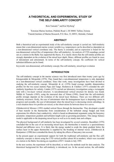
4Tamsalu & Myrberg MERI No. 37:3-13, 1998profiles will be shown and the results of the analyses of experimental data will be compared with theory.In the last section, the main conclusions of the study will be given.The reader interested in self-similarity in more detail is referred to the papers of Barenblatt (1996) andTamsalu & al. (1997).1. MATERIAL AND METHODS1.1 Theoretical derivation of the flux self-similarityThe vertical structure of temperature in the seasonal thermocline will be written in the following form:where:∂T∂q=− (1)∂t∂zT(z,t) is the temperature, q = w' T' is the temperature flux, t is time, z is the vertical coordinate directeddownwards. Substituting the non-dimensional coordinate:z−h()tς=H−h()tequation (1) can be written as follows:(2)∂Th T q( H−h) −( − ς)∂ ∂ ∂1 = −(3)∂t∂t∂ς ∂ςwhere:h(t) is the thickness of the upper mixed layer and H is the bottom of the seasonal thermocline. The followingexpression for the non-dimensional temperature (θ) and for the non-dimensional temperature flux(Q) are proposed:T1() t −T(, t z)θ=T()t −1T H(4)Q q h() t − q (,=t z )q () t −qhHwhere:T 1 (t) is the temperature in the upper mixed layer, T H is the temperature at the bottom of the seasonalthermocline (z=H), q h (t) is the temperature flux at the level z=h, q H is the temperature flux at the levelz=H. Here we suppose that q h (t) >> q H . Then (5) can be written as follows:(5)Q q h() t − q (,=t z )q () thUsing (4) and (5a), equation (3) takes the form:(5a)where:( 1−θ) 1 −( 1− ς)∂θ ∂Qaa2=∂ς ∂ς(6)

A theoretical and experimental study of the self-similarity concept 5a1H−h∂T=q ∂th1; a2TH−T=qh1∂h∂tIf a 1 and a 2 are constants, then θ and Q are functions of ς only. We start to investigate this problem fromequation (3). Vertically integrating (3) with respect to ς between the limits of 0 and 1, we get:where:1T = ∫Tdς0( H − ∂Thh) ( T T)t− − ∂∂t= q 1(7)∂hThe double integration, first between the limits of 0 and ς and then between the limits of 0 and 1 givesthe following results:where:~1 ςT= ∫dς∫Tdς0~∂T~ ∂h( H−h)−(2T− T1 ) = qh−q(8)∂t∂t0Using the relationship:and q = ∫qdς110~2T−T1=α 0(9)T −Twe get from (7) and (8) the following equation:a1where:T−T1κ=T −THα02 0 2− a2= − α−01 − α 1−α 1 − α β (10)10; β 0 = qq h0 0For the determination of q h we use the well-known relationship for entrainment (Phillips 1977) in theform:−1hqh =−c0( T −T1) ∂ ∂twhere:c 0 is a proportionality constant. Using (11) a 2 takes the form:(11)a2c0=− (12)κEquation (10) then takes the form:a= ( 2− α ( 1+ c ) −2β )/( 1−α )(13)1 0 0 0 0

8Tamsalu & Myrberg MERI No. 37:3-13, 1998probably, some of these were not "pure" type-B profiles, which is shown by the large scatter of the lattercurves. The 61 type-A curves (Fig. 2a) show a better fit with the theoretical curve and less scattercompared to case B. This is clear, because the number of profiles is large and most of the time the mixedlayer evolution was of type-A.The above analysis of the results shows that the self-similar profile (type A or B) of temperature is not soclearly visible instantaneously. Mälkki & Tamsalu (1985) pointed out that κ only reaches a constantvalue if an integration over the inertial period (about 14 hours) is carried out.The vertical flux of temperature wT ′ ′ has been calculated according to (14). The fluxes are presentedseparately for cases A and B as a function of ς . The most striking feature is that the shapes of the fluxprofiles differ clearly from each other. In case A the flux has its maximum value near ς=0 anddecreases towards ς=1 (Fig. 3a), while in case B (Fig. 3b), the maximum flux is reached betweenς= 02 . −03. , decreasing again towards ς=1.After deriving the vertical flux of temperature wT ′ ′ , a vertical integration of the experimentally-derivedprofiles is carried out. We investigate here only case A.The calculated values of α 0lie between 0.69-0.82, and we take α 0=0.75. The calculated β 0was 0.61,and we take β 0=0.6. The calculated values of κ lie between 0.72-0.77, and we take κ=0.75. This canalso be found by integrating (4) using (15):1T1() t −T()t∫ θς d == κT()t −01T HIntegrating (6) with respect to ς , we get:(17)ςς⎛ ⎞⎜ς−∫θdς⎟a1 −(( 1− ς) θ+∫ θdς) a2= Q(18)⎝ ⎠0Integrating (6) between the limits of 0 and 1, we get:0( 1−κ)a − κa = 1(19)1 2Substituting the values of α, β and κ into (12) and (13) we find, using (19), that c 0 =3.8,0 0a 1 =-11.2 and a 2 =-5.07 (20)Substituting (15) and (20) into (18) we get the following expression for the temperature flux Q:4Q = 1−( 1−ς )(21)The temperature flux can be written in the traditional way as follows:qT=−ν ∂ ∂z(22)

A theoretical and experimental study of the self-similarity concept 9Fig. 2. The non-dimensional temperature θ plotted against the non-dimensional vertical coordinate ς .The curves based on observations are marked with dotted lines. The theoretical curves are markedwith continuous lines: A -the mixed layer depth is increasing, B -the mixed layer depth is decreasing.

A theoretical and experimental study of the self-similarity concept 11Using (15), (21) and (22) we get the following equation for the coefficient of vertical turbulent diffusionν:1 − ∂∂υ=− −ς= − −ς2 1 2 H h h( )∂01 h. *( H h) (∂1 )a tt2If the diurnal change in the upper mixed layer thickness is 1 m, and the thermocline thickness is 30 m,then:ν=0.3 cm 2 /sat the top of the thermocline.For practical use, equations (23) and (9) are the most important ones.The non-dimensional vertical fluxes of temperature as a function of the non-dimensional vertical coordinateς are presented in Figure 4. The theoretical curve corresponding to (21) is marked Q 2in caseA (Fig. 4a). The experimental non-dimensional vertical flux is marked as Q 1. The corresponding approximatecurves for detrainment (case B) are shown in Figure 4b. A comparison of the experimentalresults with theory has the same main features as in the case of the traditional self-similarity concept. Incase A, the observations fit well with theory.3. DISCUSSION AND CONCLUSIONSThe traditional self-similarity concept as well as the extended theory of self-similarity of vertical fluxeswere compared with calculations based on an analysis of observations. In general, the observationssupported the theory. However, the four-day expedition was far too short to gather an adequate data setof CTD profiles in different stability conditions of the air-sea interface with respect to the evolution of themixed layer thickness.The self-similar profiles for temperature based on the observations showed that different kinds of profilesexist depending on the evolution of the mixed layer, with different profiles being found for cases ofentrainment (case A) and detrainment (case B). The observational proof for the self-similar structure oftemperature was better in case A, while the profiles representing case B gave less satisfactory evidence.This is partly because of the small number of case-B profiles measured. On the other hand, most of thetime case A conditions dominated, and profiles representing case B were not always pure; i.e. someprofiles represented the transition between detrainment and entrainment. However, self-similarity oftemperature becomes visible if a time-integration over an inertial period (about 14 h ) is carried out (seeMälkki & Tamsalu 1985).The profiles of the vertical temperature fluxes showed a clear difference between cases A and B. Thenon-dimensional fluxes of temperature also showed differences in the profiles based on the evolution ofthe mixed layer depth. In case A, the fit of theory with observations was better than in case B, thereasoning for this being the same as in the case of the self-similarity profile for temperature.In the case of an entrainment type of profile, the coefficient of vertical turbulent diffusion can be solvedin the stratified layer using the flux-self-similarity concept. Thus, the self-similarity concept can be usedas a tool to parameterize the vertical turbulence in numerical modelling.2(23)

12Tamsalu & Myrberg MERI No. 37:3-13, 1998Fig. 4. The non-dimensional vertical flux of temperature Q plotted against the non-dimensional verticalcoordinate ς . Curve Q 1 is based on experimental results, while curve Q 2 is based on theoretical calculations:A -the mixed layer depth is increasing, B -the mixed layer depth is decreasing.

A theoretical and experimental study of the self-similarity concept 13REFERENCESBarenblatt, G. 1978: Self-similarity of temperature and salinity distributions in the upper thermocline.- Izv., Atmospheric and Oceanic Physics, No. 11, 820-823 (English edition).Barenblatt, G. 1996: Scaling, self-similarity, and intermediate asymptotics. - Cambridge texts in appliedmathematics, Cambridge University Press, U.K., 386 pp.Kitaigorodskii, S. & Miropolski, Y. 1970: On the theory of the open-ocean active layer. - Izv., Atmosphericand Oceanic Physics, 6, No. 2, 178-188 (English edition).Linden, P. 1975: The deepening of a mixed layer in a stratified fluid. - J. Fluid. Mech., 71, part 2, 385-405.Miropolski, Y., Filyushkin, B. & Chernyskov, P. 1970: On the parametric description of temperatureprofiles in the active ocean layer. - Oceanology, 10, No. 6, 892-897 (English edition).Mälkki, P. & Tamsalu, R. 1985: Physical features of the Baltic Sea. - Finnish Mar. Res. No. 252,110 pp., Helsinki.Nõmm, A. 1988: The investigation and simulation of the thermohaline structure in the open part of theGulf of Finland. - PhD-thesis, Leningrad Hydrometeorological Institute, 242 pp. (in Russian).Osborn, T. & Cox, C. 1972: Oceanic fine structure. - Geophys. Fluid Dyn., 3, No. 5, 265-354.Phillips, O. 1977: Entrainment. - In: modelling and prediction of the upper layers of the Ocean (Kraus,E.B.) Pergamon Press, Oxford, pp. 92-101.Reshetova, O. & Chalikov, D. 1977: Universal structure of the active layer in the ocean.- Oceanology, 17, No. 5, 509-511 (English edition).Tamsalu, R., Mälkki, P. & Myrberg, K. 1997: Self-similarity concept in marine system modelling.- Geophysica, 33(2): 51-68.Zilitinkevich, S.S. & Rumjantsev, V. 1990: A parameterized model of the seasonal temperature changesin lakes. - Environmental Software, Vol. 5, No. 1, 12-25.Zilitinkevich, S.S. & Mironov, D. 1992: Theoretical model of the thermocline in a freshwater basin.- J. Phys. Oceanogr., Vol. 22, No. 9, 988-994.