Algorithmic Thermodynamics

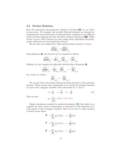
4.3 Further RelationsFrom the elementary thermodynamic relations in Section 4.1, we can derivevarious others. For example, the so-called ‘Maxwell relations’ are obtained bycomputing the second derivatives of thermodynamic quantities in two differentorders and then applying the basic derivative relations, Equations (7-9). Whiletrivial to prove, these relations say some things about algorithmic thermodynamicswhich may not seem intuitively obvious.We give just one example here. Since mixed partials commute, we have:∂ 2 E∂V ∂S ∣ = ∂2 EN∂S∂V ∣ .NUsing Equation (7), the left side can be computed as follows:∂ 2 E∂V ∂S ∣ = ∂∂EN∂V ∣S,N∂S ∣ = ∂T∣V,N∂V∣S,NSimilarly, we can compute the right side with the help of Equation (8):∂ 2 E∂S∂V ∣ = ∂∂EN∂S ∣V,N∂V ∣ = − ∂PS,N∂S ∣ .V,NAs a result, we obtain:∂T∂V∣ = − ∂PS,N∂S ∣ .V,NWe can also derive interesting relations involving derivatives of the partitionfunction. These become more manageable if we rewrite the partition functionin terms of the conjugate variables of the observables E, V , and N:β = 1 T , γ = P T , δ = − µ T . (11)Then we haveZ = ∑ x∈X−βE(x)−γV (x)−δN(x)eSimple calculations, standard in statistical mechanics [22], then allow us tocompute the mean values of observables as derivatives of the logarithm of Zwith respect to their conjugate variables. Here let us revert to using overlinesto denote mean values:E= ∑ x∈Xp(x)E(x)= − ∂∂β lnZV= ∑ x∈Xp(x)V (x)= − ∂∂γ lnZN = ∑ x∈Xp(x)N(x) = − ∂ ∂δ lnZ14