CalCOFI Reports, Vol. 11, 1967 - California Cooperative Oceanic ...

STATE OF CALIFORNIAMARINE RESEARCH COMMITTEE

This report is not copyrighted and may be reproduced inother publications provided due credit is given the CaliforniaMarine Research Committee, the author, and thereporting agencies. Inquiries concerning this report shouldbe addresed to the State Fisheries Laboratory, CaliforniaDepartment of Fish and Game, Terminal Island, California90731.EDITORIAL BOARDJ. L. Baxter, ChairmanE. H. AhlstromJ. D. lsaacsP. M. Roedel

STATE OF CALIFORNIADEPARTMENT OF FISH AND GAMEMARINE RESEARCH COMMITTEECALIFORNIACOOPERATIVEOCEANICFISHERIESINVESTIGATIONSVolume XI1 July 1963 to 30 June 1966Cooperating Agencies:CALIFORNIA ACADEMY OF SCIENCESCALIFORNIA DEPARTMENT OF FISH AND GAMESTANFORD UNIVERSITY, HOPKINS MARINE STATIONU.S. FISH AND WILDLIFE SERVICE, BUREAU OF COMMERCIAL FISHERIESUNIVERSITY OF CALIFORNIA, SCRIPPS INSTITUTION OF OCEANOGRAPHY1 January 1967

This volume is dedicated to JULIAN G. BURNETTE, Member of the Marine Research Committee since its inception in 1948and Chairman, 1948-1967.The work reported upon in this volume and all those preceding it was done during the period of his leadership.Much of the credit for the scientific advances that we have made belongs to him. His continued interest, wholeheartedsupport, early understonding of the necessity for a broad examination of the ocean environment, and, particularly, his farseeinginsight into the delicate balance between freedom and obligation in research, created an almost unprecedented rapport betweenmen of science and of practice; an intellectuol environment in which both basic scientific progress and practical results becamepossible; and a high goal for future research programs.

RONALD REAGAXGovcriwr of the Slate of CaliforniaXacranzento, CaliforniaLETTER OF TRANSMITTALJanuary 1. 1967Dear Sir: Ve respectfully submit the eleventh report on the work of theCalifornia Cooperative Oceanic Fisheries Inrestigations.The report consists of three sections. The first contains a review of the administrativeand research activities during the period July 1, 1963 to June 30, 1966,a description of the fisheries, and a list of publications arising froni the programs.The second section is comprised of papers prepared for a special symposiumon anchovy biology. The third is comprised of original scientific contributionswhich are either a direct result of CalCOFI research prod orams, orrepresent research directly pertinent to resource dcvelopment in the pelagicrealm of California.Respectfully,THE XAKINII: RESEARCH COXMITTICEJ. a. BURNCTTE, ChairmanEDWARD 17. BRUCE, Vice ChairnzanC. R. CARRYR. E. CIrilPnimIt-. M. CHAPMAXJOHN HAWKARTI-IUR H. hhND0NCA4,4hTT€IONY NIZETICHJOSEPH L. OLIVIERI

CONTENTSI. Review of Activities Page1. Review of Activities July 1, 1963-June 30, 1966 _______-______--__ 52. Review of the Pelagic Wet Fisheries for the 1963-64, 1964-65,1965-66 Seasons ............................................... .213. Publications ................................................. 2211. Symposium on Anchovies, Genus EngraulisJohn L. Baxter, Editor _______-________________________________271. Oceanic Environments of the Genus Engraulis around the WorldJoseph L. Reid, Jr.--- ........................ -________________292. Synopsis of Biological Information on the Australian AnchovyEngraulis australis (White)Maurice Blackburn ___________________________________________ 343. A Note on the Biology and Fishery of the Japanese AnchovyEngradis . .. japonica (Houttuyn)Xtgezta Hayasi .................................. -_______-____444. Present State of the Investigations on the Argentine AnchovyEngraulis anchoita (Hubbs, Marini)Janina Dz. de Ciechomski ...................................... 585. Influence of Some Environmental Factors upon the EmbryonicDevelopment of the Argentine Anchovy Engraulis anchoita ( Hubbs,Marini)Janina Dz. de Ciechomski ...................................... 676. Investigations of Food and Feeding Habits of Larvae and Juvenilesof the Argentine Anchovy Engraulis anchoitaJanina Dx. de Ciechomski ..................................... 727. A Brief Description of Peruvian FisheriesW. P. Doucet and H. Einarsson ..................... -____-____ - 828. Preliminary Results of Studies on the Present Status of the PeruvianStock of Anchovy (Engradis ringens Jenyns)G. Xaetersdal, J. Valdivia, I. Tsukayama, and B. Alegre ____________ 889. An Attempt to Estimate Annual Spawning Intensity of the Anchovy(Engraulis ringens Jenyns) by Means of Regional Egg and LarvalSurveys during 1961-1964H. Einarsson and B. Rojas de Mendiola .......................... 9610. The Predation of Guano Birds on the Peruvian Anchovy (Engraulisringens Jenyns)R6mulo Jordcin ________-. .................................... 10511. Summary of Biological Information on the Northern AnchovyEngradis mordax GirardJohn L. Baxter______________-___________-___-__-_--~___--_-_- 11012. Co-occurrences of Sardine and Anchovy Larvae in the CaliforniaCurrent Region off California and Baja CaliforniaElbert H. Ahlstrom __- ........................................ 11713. The Accumulation of Fish Debris in Certain California CoastalSedimentsAndrew Xoutar .............................................. 136111. Scientific Contributions1. The Pelagic Phase of Pleuroncodes planipes Stimpson (Crustacea,Galatheidae) in the California CurrentAlan E. Longhurst _____________-__________________________-__ 1422. Summary of Thermal Conditions and Phytoplankton VolumesMeasured in Monterey Bay, California 1961-1966Donald P. Abbott and Richard Albee ........................... 1553. Seasonal Variation of Temperature and Salinity at 10 Meters in theCalifornia CurrentRonald J. Lynn ________________________________________-_-___ 157(4)

PART 1REVIEW OF ACTIVITIESJuly 1,1963-June 30,1966INTRODUCTIONIt has become increasingly apparent that the policyof the CalCOFI has been a valid and valuable onethatthe intensive long-term study of the CaliforniaCurrent has constituted a nucleus and raison d’6treof an expanding research and technology of greaterdepth, field and compass in the North Pacific. Thenature of these expanded portions of the programare discussed later in the reports of agencies.The CalCOFI Committee is deeply involved withits fundamental objectives and with reappraisal ofthe direction that the CalCOFI should now take.This reappraisal is necessitated by the delineationof unutilized fish resources of the eastern NorthPacific and the initiation of a fishery one of thesetheanchovy.The philosophical, scientific, and politico-economicfactors pertinent to this reappraisal cannot be competentlydiscussed here. However, the crucial questionscan be reasonably well formulated as follows :Are the long-term needs of the state, society, andmankind best served at this juncture by a concentrationof research on the anchovy and its fishery orby a continued expansion of the research into thetotal environment ?The resolution of this problem depends upon avalid understanding of the evolving position of California; its changing responsibilities to its peopleand to its challenges and opportunities; and the presentand potential contribution of the CalCOFI to theState.On the one hand, as a result of CalCOFI research,we have the opportunity of reestablishing a reductionfishery of some magnitude. On the other hand, we havethe demonstrated, suspected, and as yet unrecognizedopportunities and implications of the Pacific and ofthe expanding research into it, of which the anchovyfishery is an early product.Clearly the rational solution to these mutually exclusiveextremes is an optimum attention to each-ajuste milieu in which the anchovy fishery is substantiallydocumented and studied and, at the same time,the research continues to be directed toward a broadscaleinquiry into the eastern North Pacific, its oceanography,zoogeography, history and fish populations.BACKGROUNDThe CalCOFI program, thus, plans a thoroughcoverage of the California Current system each threeREPORT OF THE CALCOFI COMMITTEEyears (1969 next), and a continuing expansion ofthe several programs, descriptions of which follow.Early in 1966 the CalCOFI Committee, in a letterto the Chairman of the Marine Research Committee,outlined the history, accomplishments, and status ofthe CalCOFI research program in simple, brief, factualterms. The 13 points, to which we referred as“a few of the many unshakeable pillars of certainty”,were :(1) The CalCOFI program was established as a broad andthoughtful inquiry into the environment and the biologyof the California Current system.(2) An object of the program was to clarify the nature ofthe decline of sardine abundance and to understand thenature of the other organisms associated with the sardinein the California Current system.(3) Organizationally, the CalCOFI is established as a groupof cooperative research programs responsible to theseobjectives and subject to the review of their progressby the Marine Research Committee, a highly selectedgroup of interested, practical men.(4) As will be enumerated below, this arrangement hasproven to be extremely successful and rewarding. Therapport between men of scientific and practical bentshas, we believe, been unique. There has been neitherconstraint, on the one hand, nor lack of direction, onthe other but rather an almost wholly unprecedentedbalance between the two where the scientist has beenable to work with “responsible freedom” and where he,the MRC and the public have been highly rewarded.(5) The oceanography, the biology of the California Currentsystem, and the variations in these are now thebest documented and best understood of any oceanicarea in the world.(6) The understanding of fish populations, biology and resourcepotential through studies of eggs, larval andadults of pelagic fishes are the most highly advancedof any.(7) Wholly new technologies of studies of pelagic fish havebeen developed and are of far-reaching, world-wide import.(8) Entrees into the pre-fishery history of the pelagic fishpopulations and environments have been developed andare of great local and world-wide significance.(9) The populations of a large group of pelagic fish havebeen determined, studied, and understood to a degreethat far surpasses any similar studies in the w-orld.The interrelations between competing species of pelagicfishes have been characterized for the first time in history.Possibility of n pelagic fishery has been pointed outand the fishery has been established, in which there is afar greater fund of scientific understanding and knowledgeavailable at its outset than for any other pelagicfishery in the history of man.A program exists that is ably discharging its full responsibilitiesboth present and future in cooperativeresearch.

6 CAIJFORNIA COOPERATITE OCESNIC FISHERIES INVESTIGATIOTiS(13) These responsibilities inclnde the study of tlie effectsof the present fishery and the inquiries essential to fnturedevelopment and iinderstnnding of other and cxtensiveresources.The .ibove are overly siniplificd statements of a part of alarge and important progrmn. We believe the results of thisprogram can be chnriwterized by stating that new and importantconcepts in the uses of our living oceanic resonrceshave been evolved. These, together with the resources atour door, hare put California ou the threshold of increasinghcr wealth, and perljaps more importantly, of assnmingworld leadership in the scientific iise of pelagic fish resources.This may, in the long run. be n far more valuableasset to Californians than the ccononiic yield of the resourcesthemselves.It TV~S on the basis of the research program describedin the above letter that we had prepared forthe Marine Research Committee, 2 years earlier, anoutline of one possible n-ay to enter this new era.This proposal mas presented to MRC in Blareh, 1964by the CalCOFI Committee which at that time wascomposed of G. I. Murphy, J. D. Isaacs, J. I;. Baxter,and E.H. hhlstroni and appears as Document XI1of the minutes of that meeting. It seems appropriateat this time to publish the proposal for all to study,evaluate, and comment upon. In the following it isquoted essentially verbatim.REQUIREMENTS FOR UNDERSTANDING THE IMPACTOF A NEW FISHERY IN THE CALIFORNIACURRENT SYSTEMOur philosophict~l guide in preparing this discnssion hasbeen simple. We hare asked ourselves, “How should afisherj- be condiicted, 2nd what investigations should beinitiated to give the public guidance of maximuni valuefrom marine science?” Ke would like to regard a newfishery on the sardine-anchovy system as n careful scientificexperiment? in which the effect of a controlled harvestof the anchovy and snrdinc poliidations is explored. We believethis is a new :uiil stimulating point of departure.While we do not propose it to ~OLI as ii necessary courseof action, we hope you will examine it thoughtfully anddecide for yoiirselves the estent to which the scientific reqiiirementsfor siich an experiment are compatible miththe broad needs of society.Background RdsumCThe resiilts of over 40 years of study, including 14 yearsof very intensive inqiiiry can be succinctly snmmarized asfollows : After many years of intensive selective fishing forsardines, the sardine popnlation declined. This decline wasaccompanied by a drnniatic npslirge of :in ecologically siini-Iar species, the anchovy. The decline of the sardine ims apimentlythe result of an intensive fishery together with aseries of years in Tvhicli the eiivironmental regime was unf:m)mbleto tlie sardine. The rise of the anchovy is apimentlythe result of a series of favorable Sears for tli:~tspecies, and nxin’s removal of sardines xvhicli created moreliving space for anrhovim The cvideiice does not allow listo :wive :it a conseiisns :IS to ~hether or not the anchoviesaggressively drove do\vn the sardine population, bot1)iologic:il interaction brtlx-een these ecologically similar slwcies is strongly inclicatcd now by the faihirc of the sardineto resiiond to a recent spectrnm of oceanographic conditionsthat should have been favorable, and conrerscly nnf;ivor.iltleto the :inchovy.Tn :ins- event results of all these stndies sho\v that thereis 110:~ :I Imgc unused popiilation of anchovies. They alsoinfer that there is a real chance that simultaneously reducingthe pressure 011 sardines and imposing pressure onanchovies will reverse the present equilibrium and assistin bringing back the more valuable sardine. This constitutesan exciting opportnnity for marine science to assistsociety in nrcetinp its coml~lcz ntwls.Requirements for the FisheryIn developing this section three factors have been paramoiunt.1. The basis for the suggested experiment while the mostcomplete ever achieved still is not precise enough to foreseeexactly how many anchovies and sardines should ultimatelybe taken. A c;weful, step\%-ise, approach such :ISv-as used in Sonth Africa is the only defensible experiment.2. There :ire time lags in the response of fish populationsto new factors. With respect to sardines and anchovies.their life histories suggest that at least 3 years wonldbe reqnired for tlie responses of the popu1:ltions to be cletectecl,even in a rcyime of favorable environments.3. There are also time lags in scientific analysis, theseare especially significant when dealing ix-ith a new problem.Thus it is necessary to carry out mcnsnrcments thatcan follow events closely, and which vi11 yield results thatars readily interpreted. With these factors in mind theaplironch helow is divided into phases. JVe believe thatthree years is a niinimiim for each lihase.Phnse 1. The objective is to initiate :I conserv;itire fisheryon :rnchovies arid rediice sardine fishing just suffieientlSto prodiicc an o1xerv:rble change in thc system, and justenorigh to improve our preliminnry appraisal of the niagnitudeof the anchovy resource. During this phase a limitof 200,000 tons should be placed on the anchovy fisheryand the sardine fishery should be limited to 10,000 tons.Thirty-five percent of both of these limits shonld be takenoff California and 65 percent off Baja Cxlifornia.1 Fromthe viewpoint of conchicting a controlled experiment, itwodd not be dcsirnble to place n complete moratoriumon s:irdines for two reusons. The fishery is a primary toolfor detecting responses in the sardine population. Werethe fishery terminated this tool would be lost, and we~vonld have to rely entirely on our surveys. Secondly,conip!ete nioratorinm would complicate the experimeiit byintrodiicing two variables at the same time. The limitsuggcsted for the sardine relieves these problems by keepingour “ivindo\v” on the sardine population open, and bgapproximnting the average rate of exploitation prevailingover the past years. If both the sardine fishery and cnin1)etitionfrom michovics are affecting the sartline l>opnlation.the chances of bringing baclr the s:irdine in the shortestpossil)le tinie can be maximized by fishiiig for anchovies andiiot fishing Cor sardines. If this is the objeclive it might bedesiyahle to ha~e n mor:itoriiim on sardine fishing. The recoiiinieiid;i~ioiisof this rc1)ori :ire b:is~d oii the viewpoint ofcondncting as careful :in esl)rriineiit :is Imssible to determinethe fact orx ;iffec.ting Imth s;trdiiic.s and nnchories.Phctse ,?. The :iinoiints to h removed dnring Phase 2and the :irenl distribntion of the limits on each speciesmust nwait the resiilts of I’hnse 1. We can hazard a guessthat tliniiip this l’hnsr thc :iiicliovy qnot;i might l ~ wisctlx:il)out 50 1)c’rcc’iit pi~~vi(liiig t1t:it the Irsiiiir of Phase 1 areiiot v%lelj- different froin our l,relinlinnry expectations.Pitrtxe 3. This cannot lie specified nt all beyond indicatingtlie nltiniate objectivc. ‘Phis is to restore the predeclineb:ilarice lwtwxii sardines and anchovics, and masimizrtlici harvests coiisistcnt \\-it11 nll nses, Le.: food, recreation,etc.C”oiv)u(wt: It is 1 ~ ond 3 oiir NCOJ)C to tlctc~rmine 1:ow siich.trni of ni:iit:i~rmrnt 01: ai! iiiterit:itional retroi,g13.tl1at conserv~l-RECENT DEVELOPMENTSThe 1964 proposal also outlined the basic programsrTThicli should be iinplemrnt,ed if a fishery were initiated.At that, time no fishery for anchovies existed,except for the limited (qlOO-6,OOO t,ons) fishery for1 At the ’21 May 1964 meeting of the LParine Research Committee,CalCOyI rbcorded the following emendation : ‘‘Our recommendationfor Phase 1 included a pro\-ision to distribute thecatch between Alta and Baja California. For the purposes ofthis pro\’ision we specify 31”s latitucle, as this is a naturaloceanographic and faunal boundary.”

REPORTS YOLUAIE SI, 1 JULY 1963 TO 30 JUSE 1966 7lire bait. 3s a direct result of the CalCOFI proposal,the Califoriiia Fish and Game Coiiimissioiiauthorized an experimental aiichovy reduction fisheryon Norember 12, 1965. The 75,000 ton quota allo~redi4 appro~il~~i~tely of the magnitude recommcndd forCalifornia waters by CalC'OFI. This fishery Iinscontinued to the present time (1967).In Mal-cli. 1966, with tlie fishery nndcr~my, E. H.Alilstroin updated the 1964 propos:il to poiiit up tliebreadth and pertinence of CalCOFl 1-esearcli to present and lonp-ranq problems. The followi~ig is hisoutline of tlir programs implenieritccl :STUDIES ON THE FISHERYImportant information can he gained from the fisherynhont the quantity of fish landed, size and age compositionof landings, and catch per unit of effort. Other kinds ofinfornintion thnt can be derired from sgstem:rtic samlilingincliide grolvth rate, age at first niatnrity. longevity,yield per recruit. mortality estimates, etc. Tliese :ire "coiiventional"investigations. involving fairly stand;irdixedtechniqiies. h fishery carried out at a low level of intensityfnrnishes only limited dnta for (letcrminiiig vit:rl stntistiesof tlie popnlation being fished. Such studies areof greatest v:diie in detcrinining vital l)ognl;itioii 1)arnnieterswhen curried oiit over different levels of fishing iiitensit>-.Total Landings by AreaC'n!iiorrr ia E'isircry: Ihiidiiigs statistics now oht:iiiicvl hythe Statc cover tonnage landed. are:r of rapture. and fishingeffort. Accnrate weights are rq)orted on market arid ci111-nery recri1)ts :IS reqnired Iiy law. ,\rea of catch is deterniinedfrom linliing iogs. reqnired of e:icii hoa t skipper,wlierc~!)y r:icli dtiy's fishing is plotted on :I map-type log.Bo jcc ('r/Eifornia >'ishc ry: I'lant o1)er:itors in Bnja Califoriiiacooperate hy giving tis :>ccess to 1:indiiig rocords.rinntioii abont aw:i of captureSize and Age Composition by Arearhlii cwncerning size and age corii~iosition are o1)taiaedby systcmatically sampling commerci:rl 1:undings from :illports of laniding in Cirliforiiia nnd Bxja California. S:iniplinxof comnierci;il Iniiciings in Califoriiia is cnrried oirt hythe ('aliforni;~ Degnrtmciit of Fish and G;ime. Samplingof comnirrcinl landings in Bnja ( lifornin is e:irriecl onthy the I~nre:~n of Cornmercial E' lieries by meiiiis of acontrnct with the California A\c:rdrniy of Scicnces. Samplesof v-iio!e. iidiilt fish will hc retaint4 for 1lnforesee:rl)lerenc:ircli. Age determin:itions :ire (lone coopcr:itiveIy liy (-":~liforniaI )rlmtment of Fish :mtl Game and Bnrenn of Conimerci:ilP'isherics scientists. C'ooperntive nging of sardinesby tlitw two organizations dates from 1941 ; coolicr;iti\-eaging of :inellovies from the e:irlj- 1950's.In the past, srnles liaw Iiwn "read" to determine tlieage of both sardines and ;nicliovics. l'resenll~-, cv:~lnationis tieing ni:ide of the acalr iiirtliod for clctrrniiiiiiig ageversns I;SP of car holies (otoliths). Anchovy scales arehighly dwidnons, 71-ith the resnlt that it is difhciilt to 01)-tain ndeqnnte scale samplcs from some loads of fish. Sanplingcan he carried ont more systeninticall>- if hiset1 onotoliths.Catch Per Unit of Effort by AreaC';ilifornin lins institnted a loghook system to olitnin informationconcernin: e:ich commercial 1:inclings of :mchovies.This is in :iddition to information olit:iiiird by intcrviews.wliriiever a 1o:id of fish is sanilrlcd.It prwrntlj- is not fe:isible to try to institate n logbooksystem for Baja Califoinia fishermen. We are able to obtainiwolds of initivitlrial d(~liwric~s. and to snpplementthis by interviews.STUDIES ON THE POPULATIONSOne of the major reasons for esta1)lishing ('alC'OF1 wasto ohtnin information about many aspects of the populationdynamics of the sardinc that conld not be wriiiig ont ofc;itcli and effort data. l\lethods independent of the fisherywere rlereloped to determine popnlatioii sizc. popdationstrnchire, factors iinderlying marked fiuctnations in tliesnrvival of yenr-classes, shifts in distribntion of the populationwith respect to the area of the fislierj- (availability I,etc. What \vas not fnlly appreciated was the complexityresnlting from competition het\veen species of a trophiclevel (Le. betwcen s:~rdine and anchovy).We mnst continue to inwstignte tlir inter:lrtion betweencompeting species. This rcqiiires more so1)llisticated researchthan is Iiossihle from stndies on the fishery alone.Tagging Experiment-AnchovyThe State lins already initiated a tngging experiment insonthern California waters. They had tagged aboiit 100,000anchovies 1)s Xovem1)er. 1966, in arexs off northern BajaCalifornia, sonthern California (inshore and offshore) andtlir JIontereq- nay area. I~~vent~rally n tagging esl)eriiiirntshonltl permit a cletermin:~tion of the extent of migrationsnntl intermiiigling of fisli from vnrioiis parts of the anchovies'range-California, Raja California or the PacificSorthwest. Tagging esperiineiits should be combined withgenetic stndies. Tagying on n broader scale may provideinformation almit popnlation pnr:tmeters snrh :is popnlntionsize. fishiiig mortality. and ii:itnr:il mortalit y.One of the initial problems we 1i:rrc to clncitlnte is tlieextent and rate of repleiiisliment of stocks from otherareas. Will fish move iip from Baja California for csnniple.to rcpleiiisli stocks reduced by fishing off sontliern Califoriki'?h very siiccessfiil tagging experiment ~-ns carried onton the Pacific sardine (1936-41). mostly liy the C'aliforninJ)epmtment of Fish and Game. The lkpartment vi11lie chiefly responsible for the tngging espc~rinient on tlie:~iicIiov>-. The Enre:in of Commercial Fisheries is cooperat-1)- in dercloping tecliniqiies tlwt will wsnlt ininortality ; also in ev:iliiating this mortality.Genetic StudiesThese are necessary to cletermine v-hct!lrr one 01' severalstocks are being fishrd. IVe non- know. for cx:niiple, thatthe s:rrdii~e fishery OK sontliern California dqwntled nlrontw(i genetic stocks (northern :and sontlieri1 siil)l)ol)iilntioiis)n-it11 cliffcriiig availahilitg. Is tlie :inchovj- po1111~:1tioil in the1';icific ofl' C":rlifnrni:x ant1 Baja Cxliforiii:i siiiiil:lrly made 111,of sc\-t~~l genctirully dist irict stocks? In point of fact. :It:igging rsperinient ~vonlcl he rondiicteil qnite differentlyif we defiilitelj- I;iie\r illat tlie anclio\-y pop111:itioii consistedof :I single interniiiigliiig stock rather th:in severalgeiieticiil1~- distinct stocks.B('I

8 CALIFORNIA COOPERATIVE OCEANIC FISHERIES INVESTIGATIONSFish SurveysSurveys designed to assess the abundance of adult populationsof sardines and anchovies should be given highpriority. It is hoped that such surveys essentially willbecome as sensitive a measure of abundance as are theegg and larva censuses.Both California Fish and Game and the Bureau of CommercialFisheries have increased their research in this area.The California Department of Fish and Game is utilizingfunds obtained under the Commercial Fisheries Researchand Development Act (Bartlett Bill) to increase the coverageof their surveys of juvenile and adult fish. Theirsurveys will investigate fish populations farther to sea andat more frequent intervals than has been possible in thepast. The Bureau of Commercial Fisheries has installed aSimrad research sonar on their new vesesl, the David StarrJordm. This gear should permit an assay of the distrihutionand abundance of schools of adult fishes. Cooperativecrnises are planned by a11 three agencies for developingtechniques for “Identification of acoustic targets and pelagicfish census.”ESSENTIAL BACKGROUND STUDIESThese are given in essentially the same form as inthe March 1964 proposal.Physical Oceanographya. Monitoring program through buoys, shore stations, hydrographiccruises as needed, etc. (this should be a burdenjointly shared with other interests).b. Analytical program : Basic studies of dynamic processesaffecting the California Current system with particularattention to factors affecting anchovies and sardinesand the biota in general.Biological OceanographyThis should be a broadly based background program. Theorganisms in the California Current system must be examinedas an interacting community.a. Studies of filter feeding fish, trophic level: (Includingfood habits, predators, natural mortality rates, etc.) .This is a huge area, one in which many scientists couldlose themselves for many years. Therefore, we recommendthat sardines and anchoiies be a starting point and thatstudies radiate out from them! One of the major pragmaticobjectives of this program is to test the validityof the two species system. For example, if we lower theanchovy popnlntion some species other than the sardine mayPOP up. Other projects, eg., the egg surveys, fish surveys,and the historical snrvcy contribute to this study.b. Historical : Study sediments to ascertain “recent”oceanographic history and changes of major biological componentsof the California Current system, including fluctuationsin sardine-anchovy abundance. This history probablycan be developed to corer the last 2.000 years, possiblyon a year by year basis.Fishery Biologya. Age specific fecundit;\, mortality, etc., of importantspecics, i.e., the biological properties of sardines and anchovies,etc., that underline their inherent rates of increase,and interpretation of egg surveys.These studies are critical and must receive early emphasis.b. Adult and larval physiology and behavior: These areessential to achieve understanding of the effects of environmentalchanges on the dynamics of the community. Initialfocus should be on the sardine and anchovy.Final CommentObviously this list is not complete (for example, thebasic productivity studies underway are quite pertinent).We believe it incorporates the most essential investigationsthat offer attainable goals. It is impossible to foresee whatwill seem essential and attainable in the future. The onlything that can be done about this is to foster a groupof scientists who are responsible with respect to vital andattainable goals, and who are also responsive to newproblems, new opportunities, and to advances in the marinesciences generally.On February 27, 1967, the CalCOFI Committeeupdated the recommendations to the Marine ResearchCommittee on the development of the experimentalanchovy fishery. It finds that the basic rationaleexpressed in that document remains valid.However, the values expressed in Phase 1 of the proposedexperimental fishery have been revised on thebasis of data for eggs and larvae in the additionalyears.Phase 1 had as its objective “to initiate a conservativefishery on anchovies and reduce sardine fishingjust sufficiently to produce an observable change inthe system, and just enough to improye our preliminaryappraisal of the magnitude of the anchovy resource.”This called for a 200,000 ton annual quota,3570 of which was to be taken off “California” (northof 31”N. lat.) and the balance off Mexico (south of31”). It called for a concurrent sardine fishery at a10,000 ton level. The anchovy quota was based on eggand larva data for the years 1951-59 which indicateda total anchovy biomass of about 2,000,000 tons. Sincethat time, egg and larva data through 1965 have beenanalyzed and considerable information is available for1966. These data show that the population level forthe period 1962-66 was two to two and one-half timesas great as it was in 1958-59. At the same time, thecenter of distribution of the population has altered,so that about half is now found north of 31”N.Using the conservative 2x increase and taking noteof the northward change of the population center,the total quota becomes 400,000 tons, with an approximatetake north of 31” of 200,000 tons. Thetotal anchovy biomass is now of the order of 4-5million tons. The recommended take, 10% of theminimum, is extremely conservative but is sufficientto serve the purpose of Phase 1.CalCOFI now recommends a complete moratoriumfor at least 2 years on the take of sardines becauseof the extremely low population level. We believethat a moratorium will not have an adverse effect onthe experiment. A moratorium was not originallyrecommended for two reasons: (1) So that conditionsof only one component of the experiment (i.e.the anchory) were changed and (2) so that appropriatesamples of the adult sardine wpre obtainedfor study. However, the continued reduction of thesardine population already constitutes a significantand inescapable alteration of the conditions, andsufficient samples of sardines can be obtained frommixed catches, lift net samples, etc. Thus, neither ofthese earlier objections to a moratorium on the sardineremains valid and a moratorium is now rrcommended.The CalCOFI Committee believes that the programshould now progress in the following manner :1. The anchovy and sardine populations should becarefully monitored and studied, following, ingeneral, our previous recommendations for researchon such a fishery. Research should include

REPORTS VOLUNE XI, 1 JULY 1963 TO 30 JUNE 1966 9the appropriate egg and larva studies, catchrecords, tagging, fecundity, and food studies, etc.2. Data should be analyzed and published with allpossible expedition. Back data should be givenhigh priority.3. The populations, distribution and biology of thetotal ,pelagic fishes of the eastern north Pacificmust be much better quantified. The areas oflimited biological knowledge for each importantspecies must be clearly delineated and resolved.Examples for such limitations are :Jack mackerel-area of distribution-populationsize-fecundity.Hake-distribution of adults, food.Squid-population size, distribution, food.These are conspicuous deficiencies of the previousdata. In addition, the previous data that are pertinentto the problem must be further studied and analyzedfor the important and necessary insight they provideinto the population of these and other pelagic fishes.4. The nature and mechanisms of oceanographicand marine biological variation must be extendedfurther into the source waters of the CaliforniaCurrent. New methods and new programs willnow allow us to do this.DISC USS IO N OF RECOMME N DATl 0 NSClearly the direction of research that CalCOFI recommendsis far from a singleniinded inquiry into theanchovy. We believe that we would be serving neitherscience nor the state were we to adopt the anchovyfishery as a single object of study. Rather we are recommendingan adequate continuing and defensiblestudy of the anchovy and sardine and an expansion ofthe broad studies of the pelagic environment, whichhave paid off so handsomely. In this we believe thatwe are choosing a multilane highway into the future,which not only coincides with the scientific objectives,but serves the statutory objectives of the State and theMRC, in manifold ways.For example, if (or, perhaps, when) the State iscalled upon to defend its high seas fishery resourcesagainst the encroachment of foreign fleets, it wouldindeed present a sorry argument were it to possess aplethora of data on the anchovy and negligible quantitativedata on the saury, hake, jack mackerel andsquid, for these species also are in great abundanceand clearly attractive to international exploitation.This has been pointed out before, along with otherreasons to broaden the program at this time. For example,a monolithic approach to the anchovy could, ofcourse, result in a cul-de-sac of empty answers werethe anchovy fishery to fail for economic or statutoryreasons.-E. H. Ahlstrom, J. L. Baxter, J. D. Isaacs,and P. *I. Roedel.AGENCY ACTIVITIESCalifornia Academy of SciencesThe experimental studies of responses of the northernanchovy (Engradis mordax) to light stimuli wereextended into 1964 for additional tests with applicationof ultra-violet and infrared radiation, and concludedby the end of the same year. These studiesrevealed a few important factors that are related tobehavior. These are as follows :1. The anchovy is a phototactic animal.2. It is capable of discriminating qualitatively betweenmonochromatic (green, blue, red) andwhite lights.3. It is able to distinguish green light from blue.4. It shows a preference for the green and bluelights over white.5. It proved to be strongly negative in reaction tored light (however, the fish tolerated this type ofillumination as an alternative to total darkness) .6. It is capable of reacting differently to differentintensities of white light.The results of these studies were published in theProceedings of the California Academy of Sciences onJanuary 15, 1965 (Vol. XXXI, No. 24, pp. 631-692)under the title “Behavior and Natural Reactions ofthe Northern Anchovy, Engradis mordax Girard,Under the Influence of Light of Different WaveLengths and Intensities and Total Darkness,’’ byAnatole S. Loukashkin and Norman Grant.The investigation of food habits and feeding behaviorof the northern anchovy in California andMexican waters was initiated on July 1, 1963, andcontinued in 1966. By the end of the 1965-66 fiscalyear, 592 anchovy stomachs had been collected inBaja California, southern and central California,mostly by Anatole S. Loukashkin. Preliminary analysisof the stomach contents shows that the northernanchovy is an omnivorous feeder. It feeds on both ZOOplanktonand phytoplankton. From the scant materialat hand it is difficult to determine the degree of preferencefor one type of food over the other. It seemsthat the anchovy feeds on the available supply, regardlessof kind. The stomachs collected containedeither zooplankton exclusively or phytoplanktonicones, or both. However, the bulk of food found in thestomachs was zooplanktonic organisms, such as euphausiids,copepods and amphipods. The euphausiids werethe dominant food item. Among the diatoms consumedby the anchovy, Chaetoceros was found to be a dominantform. In some cases it contributed to 99% ofthe contents in bulging stomachs (Monterey Bay).As to the method of feeding, the anchovy is both afilter feeder, and a particulate feeder. During the reportedperiod field observations under natural conditionswere carried on during routine cruises of theCalifornia Fish and Game M/V ALASKA by AnatoleS. Loukashkin. These observations include recordsof school patterns, feeding behavior, school maneuverability,and readions to artificial light sources andfishing gear, of the sardine, anchovy, mackerels andother pelagic fishes.

10 CALIFORNIA COOPERATIVE OCEANIC FISHERIES INVESTIGATIONSCalifornia Department of Fish and GamePelagic Fish ZnuestigationsThe Department's portion of the CalCOFI Programis conducted by its Pelagic Fish Investigations.The primary responsibilities are : (i) basic monitoringof tlie pelagic wet fisheries, particularly Pacific sardine,Pacific niackerrl, jack mackerel, and northernanchovy, and (ii) conducting research vessel surveysof the pelagic and bathypelagic fishery resources ofthe California Current system.Studies of the wet fisheries include : (i) sampling ofcoiiiniercial and livr-bait catches to determine the ageaiid length composition ; sardine and anchovy age deteriiiinationsare made in cooperation with the C.S.Bureau of Coniniercial Fisheries ; (ii) interviewingfishermen aiid collecting logbook data to nie~sure fidiingeffort and determine catch localities ; and (iii) determiningthe amounts of fish landed and insuring theaccuracy of source documents in cooperation with theDcpartment 's biostatistical unit.(hod progress was made with respect to the largebacklog of age composition and fishery data on jackni:!c.kerel. This information, some dating back to 1947,1i;is been processed and the analysis of data and preparationof manuscripts is in progress. The analysisshould rereal whether the jack mackerel fishery dependsiipoii highly available year-classes and. if sucliis the case, possibly explain fluctuations in fishing successexperienced in recent years.High priority is being placed on analpsing all agecornposition and fishery data relating to Pacific mackerelwith the objectire of determing various aspects ofthe popiilation dynamics of the species. Such informationhas been only partially presented in the past andthis imrk will aid materially in understanding recentchanges in the status of Pacific mackerel.In November, 1965, the Califoriiia Fish and GameC'oniiiiission authorized an experimental iiiicliovy fislic~ryfor reduction witli a quota of 75,000 tons. To dothe research required to monitor the effects of thefishery. an expanded anchory research projrct wasestablished by the Department. Concurrent with theinception of a reducation fishery new or revised Sampling aiid monitoring procedures were needed. Previouslythc anchovy fishery was quite siiiall andsampling consisted of 30-fish samples, selected at raiidomand as convenient, and skipper interviews. Thissampling procedure continued through the 1963-66srason.Beginning November, 1963, a logbook system TWSinaugurated to obtain catch, effort, gear and fishingarea data. The chart-type logbook derised prior to the1965-66 reduction season prowd successful in fulfillingits intended purpose aiid with niiiior modificationwill continue to be used. Initial problcni~ with the lopbookswere lack of coiisistency among fishermen inrecordirig scouting time aiicl inaccuracy of the fishermen'sestimate of catch size. Both problems decreasedas the fishernieii gaiiicd experience. Data recorded inthese logbooks are coded, key punched, and machineproccssed to facilitate analAt the start of the secoiid anchovy reduction season,sanipling procediirrs wrre cah:inged rather extciisiyelj-.('hanges mere based on the kiioJTledge gaiiied durillgthe first season and will probably be modified as thefishery increases and as we increase sainpling efficiency.Briefly our southern California sampling planrequired obtaining 20 random samples for every

REPORTS YOLUME SI, 1 JULY 1963 TO 30 JUNE 1966 11California including northern Baja California. Followupcruises in southern and central California serveas both gear research cruises and intensive samplingsurveys.The first phase of the expanded survey, in fiscal1965-66, was designed to provide continuity withcruises conducted during the past and to develop thefollowing survey techniques, which have been in effectsince June, 1966. An echo sounder is operated continuouslyduring the day over predetermined transectlines that extend perpendicularly from shore for atleast 35 miles or until the 1000-fathom depth contouris reached. These lines are spaced 15-30 miles apartand average about 50 miles in length. Hourly fixes areobtained and the number of schools appearing on theecho sounder are recorded for each hour of runningtimci. Identification of species is accomplished by echotrace characteristics and by fishing x small, 30-footmidwater trawl. The trawl is also fished at regularIO-miles intervals during the night as the vessel returnsinshore over the outbound transect lines. Arecord is kept of all visually observed surface schoolsand indications of fish during both day and night.Catch records include species, numbers, sizes and sex.Scale or otolith samples are obtained Prom the imtantspecies for determining age composition. Limitedoceanographic obserrations pertaining to fish distributionare regularly obtained. These include bathytherinographcasts, water turbidities, temperatures, aiidweatlier conditions.We hare now completed five cruises of this newtype ; two to central California. two off southern Californiawhich includes northern Baja California andone in southern Baja California. Anchovies have beentlie dominant species in all areas. Since these surveyswere initiated some important seasoiial distribution andbeharioral aspects have been deterniined for anchovies.During spring the anchovy population was composedof thousands of rery sniall schools distributed overlarge areas extending at least 50 to 80 miles offshore.These schools were located near the surface in clear,deep water and normally contained less than 2 tons offish. All were adults in advanced spawning stages.Imge compact schools, suitable for purse-seine fishing,were scarce and found only in a, few localized areas.*Juvenile fish were generally found close to shore inwater shallower than 50 fathoms. During sumnier andfall all sizes of anchovies were found rniich closer toshore, at greater depths, and in larger but fewerschools. Decrease? in school numbers from spring tofill1 in th(J southern California area exreedd 80 percent.These rcsults indicate that, in general. the fishspread over a large area in spring to spawn and concentratein small coastal areas during suninier and fall.The most opportune time to estimate population sizeappears to be spring. With the large iiuinber of schoolsand extensive distribution, echo sounding surveyingis much inore effective. Schools size and identificationare also inore easily detemniined. Fall aiid suninier distributions,with fewer and large schools, decrease theeffectiveness of tlie echo sounder in probability of de-tection, species identification and school size determination.This type of distribution and behavior shouldbe more favorable for commercial fishing.School types and behavior patterns were also observed.Small numbers of horizontal-layer schooltypes 80 to 100 fathoms below the surface and morenumerous plumes located 20-50 fathoms deep werethe predominant schools in northern Baja Californiaand central California. The southern California regioncontained these types plus plume-type schools at shallowerdepths. At nightfall a11 school types came tothe surface where almost all dispersed into surfacescatter or loose detached school segments. Only a veryfew remained compact enough to be visible as a bioluminiscentspot or register as an echo trace.The night behavior of anchovies appears closely associatedwith the upper extremity of the scatteringlaper that coiners toward the surface after dark. Theafter dark rise and surface dispersal of schools suggestsa feeding behavior as eyidenced by the largenumbers of recently ingested food organisms observedin stomachs of night-caught fish. 9 very high percentageof these organisms were euphausiids, which are animportant constituent of the upper scattering layer.Quantities of sardines were present only in thesouthern part of Sebastian Vizcaino Bay. Adults ofthe fall spawning sub-population overwhelmingly predominatedthe samples taken. This group is now apparentlythe strongest remnant of the whole population.Incoming juvenile year-classes were practicallynil. Other species surveyed were minor in importancecompared to anchovies. Juyenile jack mackerel,mostly of the 1966 year-class, were widely distributedin small scattcred schools. Trawl catches usuallyranged from 1 to 50 individuals, they rarely exceededI00 specimens.Hale were locally abundant in July off San Francisco.Many- schools were found associated with whitebaitsmelt. Both species were in close association witheach other, the hake wre 1 to 3 fathoms off the bottomwith the smelt 3-4 fathoms abovc them. The hakeappeared as small groups, 20 to 50 yards apart. Aseries of these groups was counted as a school. Onesuch school was over a mile across. Those sampledwere large adults, 20-25 inches. Only minor traces ofhake were noted in southern California in Octoberand no concentrations were seen in November off centralCalifornia.The Department continued to issue data reports onpast-year cruises (since 1930). The material is codedonto IKM carcls. organized into tables by ail electroniccomputer, and printed directly by a photographicprocess. The data are printed in the California CooperativeOceanic Fisheries Investigations ( CalCOFI)Data Report series.EicL.lit reports, co~~ring the I) years from 19330through 1938, wcre printed and distribixted whik twoinore reports 19 and 10) for 1939 and 1960 Twre conpletedniid ready for printing. Data for the sevraladditional yearc, were partially processed and will beprinted as they are ready.

12 CBLIFORNIA COOPERATIVE OCEANIC FISHERIES INVESTIGSTIOX’SHopkins Marine StationThe Hopkins Marine Station of Stanford Universityat Pacific Grove, California, conducts studies onthe environment and organisms of the coastal watersof central California. Under the CalCOFI Programthe marine station monitors the marine climate andphytoplankton of Monterey Bay. Approximatelyweekly cruises to six stations are made on MontereyBay, and daily shore temperatures are reported fromPacific Grove and Santa Cruz. The data collected arecompiled and distributed to interested agencies andindividuals in the form of mimeographed quarterlyand annual reports. A short paper summarizing someof the results obtained appears elsewhere in thisreport.Scripps Institution of OceanographyMarine Life Research ProgramThe Marine Life Research Program includes thatportion of the research of the California CooperativeFisheries Investigation that is conducted by theScripps Institution of the University of California.This program has been principally concerned withthe ecology of the California Current system-that is,its currents and countercurrents, temperatures andtemperature fluctuations, and its chemistry. plankton,climatology, etc.The Marine Life Research Program (MIJRP) hasalso expanded its scope considerably through a seriesof contracts and grants from the Office of Naval Research,the Atomic Energy Commission, the NationalScience Foundation, The Marine Research Committeeand others. It also has expanded by informal cooperationwith the Navy, the Coast and Geodetic Survey,other research programs of the University, etc.In addition to the broadened research into the easternNorth Pacific, the MLR also is carrying on itsresponsibilities for the monitoring of the CaliforniaCurrent and the anchovy fishery, as discussed in theCalCOFI Statement.The MLRP thus plans a thorough coverage of theCalifornia Current System each three years (1969next) , and a continuing expansion of the several programs,descriptions of which follow.Atlases. The reduction of the load of routine datacollections, has allowed an acceleration of the analysisand publication of the data taken over the period ofintense inquiry. The last several years have thus seenthe publication of a number of atlases on the distributionand distributional changes of the principalplanktonic organisms of the eastern North Pacific.The atlases now published or in press include theCopepods of the California Current, Vol. I; the Euphausiids; the Dynamic Heights ; and 10 Meter Temperatures.Other atlases in late stages of preparationare : Copepods, Vol. 11; Biomass of Zooplankton (seebelow) ; Chaetognaths ; Molluscs ; Anchovy Larvae.Within the next year there thus will be in publishedform the most extensive biological and physical oceanographicdocumentation of any oceanic re,’ eion onearth. The atlases are published with particular attentionto the requirements of an interdisciplinarycooperative program, so that scholars in a number ofdifferent disciplines can compare distributions andcheck their hypotheses of interaction and dependency.The atlases are thus precursors of much added discovery.Biomass Analysis. In the last several years theproblems of arriving at a meaningful measure ofzooplankton have been resolved. The purpose of thebiomass analysis was to develop a measure and methodologyfor the zooplankton that would typify it asa functional component of the organic milieu. Thisis in distinction from a strict taxonomic breakdown.The nineteen functional groups are measured in volumein each sample. Thus the data from each cruisecan be presented as the actual organic component ofthe water represented by each of the groups. Thevariations between years is striking and is related tothe varying oceanographic conditions.As the zooplankton are the vital food for most ofthe small pelagic fishes, these fluctuations are particularlyimportant to the CalCOFI objectives.Biomass analysis of the zooplankton have now beencompleted for a number of years and the first atlaswill soon be published.Varved Sediment Study. As previously reported,the sediments in certain basins are apparently laiddown in annual layers and subsequently undistrubed.These sediments thus contain a “record” of almostannual resolution of the oceanographic and marinebiological conditions of the overlying waters for atleast the last several thousand years.We are thus able to reconstruct the range of conditionsto which the region has been subjected with agreatly enhanced insight. The conditions during recentstudies can be placed in an extremely importantperspective.Sediments of this type have now been found inabout six locations along the Pacific Coast fromsouthern California to central Peru.Fish scales are abundant and extremely well preservedin these sediments. The initial findings insouthern California sediments are that the sardinescales are only twice abundant in these sediments.The recent period of about seventy years was a periodof abundance and there was a similar period abouteight hundred years ago. At other times sardine scalesare rare. On the other hand the scales of the anchovyand the hake are in high abundance throughout theentire period except for short periods of time. Anchovyscales were rare in the recent period. The recentperiod appears to be typified by a weak CaliforniaCurrent.The importance of the local and world-wide implicationsof this sediment work can scarcely be exaggerated.It is an unexpected, unprecedented and potentiallypowerful entree into a very broad understandingof the distribution and variations of pelagicfishes and the related oceanographic conditions.Sediment Collections. Not unrelated to the findingsof the sediments, the MLRP has recently developeda collector that can be placed on the bottom ofthe deep ocean, and which will collect coarse particlesof sediment that are precipitating from the water

REPORTS VOLUME XI, 1 JULY 1963 TO 30 JUNE 1966 13column. Although only a few experimental sets havebeen made, from the data collected have been madethe first direct estimates of the natural generationtime of some planktonic marine organisms. It maybe that this approach can yield much fundamentalunderstanding of the economy of the sea that hasavoided other efforts.Planetary Food Potential. Included in the MLRprogram is a continuing study of the position ofmarine productivity in the food potential of thisplant. This study is, of course, highly approximate.Nevertheless it aids in placing fishery developmentin perspective. Figure 1 compares the productivity ofthe land and sea and the related harvest by man. Thepotential harvest of the sea is seen to be several ordersof magnitude greater than the present, or enoughanimal protein for more than 60 billion people. Itis clear from this study that such a harvest can beachieved only by the capture of rather primitivelyfeeding fish, such as the anchovies and sardines.In addition, the probable efficacy of such interventionsas artificial upwelling can be evaluated in such aperspective matrix. It appears that the heat rejectionrequired to produce the world’s power requirementfrom atomic sources can incidentally increase theocean productivity in an amount approximately sufficientto supply a quarter of the needed protein.F,3OCWlC *WD TWRESIRIAL loOD WaGYP c.1/)..out.ide .tmo.ph.r.L c.1IyIlNmLAT1mom Urth aurfac.1024 - *..f“l in .”1022102110201014 - Iwdul in photoi)mth..i.3.5 useful on l adFIGURE 1. Diagram of total energy cascade into the food of themarine and terrestrial realms.-prepared by W. Schmitt.I1024Details of these and other such considerations canbe found in several of the listed publications.Sardine Parasites. An. investigation into thestomach contents of sardines indicates that the sardinepopulation off California was increasingly parasitizedby two species of trematodes during the period 1925to 1955. In later years the infestations were veryheavy. There is even some evidence of competitionbetween the two species of trematodes within thesardine stomachs. Such competition would be almostcertain evidence that the infestation was damagingto the sardine.Neither the sardine below Sebastian Viscaino northe anchovy were subject to such infestations.Whether or not this infection contributed to thedecrease of sardine stocks cannot be definitely ascertained.Xea Xurface Temperature Anomalies. The Yearsof Change 1957-58, brought to our attention the factthat variations in oceanic conditions were not of localorigin but rather involve the entire North Pacific,if not the entire planet. We now know that nonperiodicdepartures from normal sea surface temperaturesare common throughout the oceans. In the NorthPacific these anomalous conditions are often largescale and of long persistence (ea. $ the width of thePacific and of 2 years duration). These anomaliesare associated with changes in weather conditions, thedistribution of marine organisms, circulation, etc.We are now planning a large-scale study of theseanomalies and their associated conditions utilizing alarge number of unmanned instrument stations overa major part of the North Pacific.In preparation for this research, a pilot study hasbeen carried out. This study has revealed a number ofhigh intriguing characteristics of these events thatwill require explanation. Among these findings are :A dependency of anomalies on the local spatial temperaturegradient over one-half of the year; a relativelysmaller variation in spatial and temporal temperaturegradients in the regions of high anomaliesthan in the regions of “normal” conditions; an anisotropyof the heating-cooling cycle ; and others.In addition, the first long-term records from unmannedstations have been obtained. These have shownseveral important features including astronomic periodicitiesof temperature fluctuations.This planned study of the North Pacific shouldresult in better insight and input into North hemisphericmeteorological and oceanographic prediction.Some of these deep moored stations will be installedin the CalCOFI area and will result in almost continuousoffshore data.Deep Benthic Conditiolzs. The oceanographic studiesof the eastern North Pacific have been extended intodeep water. The findings have been most significant.Many of the conditions of the deep ocean bottom arevirtually unexplored. The near-bottom currents arevery poorly known, and little is known of the activecreatures of the deep ocean floor. The developmentof autonomous instruments at Scripps has allowed

14 CALIFORXIA COOPERATIVE OCEANTC FISHERIES IISVESTIGATIOSSus to add some insight into these conditions. Deepcurrents in the eastern North Pacific have been foundto be low but of somewhat higher velocity than anticipated(ea. 3 cm/sec), and the fluctuating componenthas been found to result principally from the lunarsemi-diurnal surface tide. We have also demonstratedthe presence of unexpectedly large fish populations(see Figure 3) including wry large climax predators,whose presence on the deep ocean bottom is anenvironmental condition of importance.TnstrirniPnt Dcwlopwmt. Recent instrument developmentin the MLRP has been remarkably sucessful.All recent deep moorings have remained inoperation at least six months in the open sea and oneremained for 23 months. Long period records are nowavailable that greatly increase our understanding ofocean conditions and are allowing the greatly increasedprogram.The autonomous instruments are valuable for researchof the deep bottom.The new Isaacs-Brown Opening-Closing MidwaterTrawl is yielding much needed data on the verticaldistribution of marine organisms.New instruments under development include newsensors for deep moored stations, an acoustic releasefor autonomous instruments, isotherm followingfloats, etc.Special Cruises. The special cruises of the MLRPhave been directed toward : (1) instrument development,(2) exploration of deep benthic conditions includingthe varved sediments, (3) cruises to exploreand further delineate biological and oceanographicconditions in the North Pacific. Three such cruiseswere carried out in the period.Sunzniary. In summary, the MLR program overthe recent period has greatly expanded its competency,range of interest, and findings. This expansion hasbeen spatially into the North Pacific, rertically to thesea bottom, and temporally into the past range ofconditions of the California Current.This expansion is dependent upon and additive tothe knowledge and insight that the CalCOFI programhas created which is serving as a precious foundationfor an expansion of research and the opportunities ofCalifornia-and vindicating the prediction of the genitorsof the CalCOE'I program that the Pacific canrepresent a freedom to the State of California ratherthan a barrier.U.S. Bureau of Comnsercial FisheriesCalifornia Current Resources LaboratoryThe former La Jolla Biological Laboratory, theoldest Bureau of Commercial Fisheries Laboratory inCalifornia, was renamed the California Current Re-(300)................ :::::::::...................................................2nd Carnivores3rd Carnivores__---1965 Harvest(112 of catch)................ . . . .(45) ....... .; . . . . . . . . . . .6.0 x 10~79.0 x 10l67.5 x 1oI6 1.5141.2 x 10131.8 x 101.4(1)- (7) I. . .!A /.P r, / 4(0.8) -actual human consumption(0.4) -9.0 x 10 13-----1.0 x 10 13Flounders, Crabs, Lobster. Sea-stars,Fish larvae and frySquid, Salmon, Tuna, Cod. Hake,Porpoise, Skates and Rays, Sea birdsSeals, Sharks, Toothed &ales,Marlin____-_-----Herring, Anchovy, Menhaden, Cod, Hake,Haddock, Rockfish, Mullet, Tuna,Mackerel, Salmon, Flounders, Squid.Oyster, CrabsNote:The food chain should mte accurately be thought of as a foodweb, in which most organisms feed on mre than onetrophic level, changing diet with their age (especially when young) and the availability of food.FIGURE 1. Diagram showing the total marine food web. Hatched areas show total food ond total protein food at each step.-preparedby W. Schmitt.

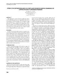
REPORTS vor,uiwIi; SI, 1 JULY 1063 TO 30 JUNE 1966 15FIGURE 3.Grenadiers, hagfish, migrating tube warms and other creatures attracted to a bait and photographed by an untethered automatic cameraat 1200 fathoms off Baja California.-(field view is about 9’ x 12’).sources Laboratory in 1964, and in September of thatyear mored from the old, frame building on theScripps campus, where it had bwn housed since 1954,to the newly built Fishery-Ocranography Center 011 itcliff site orrrlooking the ocean, $-mile north of theold location.The Center is a strikingly modern laboratory, builtof prestressed concrete and includes four multi-storybuildings around a center courtyard. Noteworthy featuresof the Center are research laboratories groupedinto functional complexes for studicJs of physiology,fish taxonomy, behavior, culturing of niariiie organisms,radiobiology, population ecology, aiid chemicaland physical oceanography. An experiinc~ntnl scilwateraqu;irium w1iic.h delivers 200 gallons per minute.ria epoxy-lined asbestos concrete and polyvinylpipe lines from the Scripps Institution of Occanograpliypier, is the focus for rearing aiid behavior experimentsand physiological studies on fish and othermarine organisms. These excellent facilities hnve madepossible some of the results discussed later, as for exanrple,tlw successful rearing of pelagic marine fishlarr~e ;ind tlic maintcnance of euphausiid shrimp incaptivity.The California Current Resources Laboratory carriesout a broadly based research program, emphasizingthe study of pelagic fishes, exclusive of the temperatetunas, in the California Current region. The oceansurrey program is carried out cooperatively with theScripps Institution of Oceanography’s Marine LifeResearch Group. With the California Department ofFish and Game, the California Current ResourvesLaboratory investigates the age and size compositionof commercial landings of sardines and anchovies, andcontracts with the California Academy of Sciences tosample the sardine and anchovy fisheries of BajaCalifornia.We have tried to acliiere a balance in the California.Current Rwources Laboratory between basic and appliedresearch. The laboratory has pioneered in sereralimportant areas of ocean research, including thetaxononiy of prlagic marine fish eggs and larvae, theusc of systematic egg and larva. surveys of oceanicareas for evaluating fish resources, the use of bloodgenetics for establishing the existence of genetic stocks(subpopulations) within the Pacific sardine populations,the rearing of pelagic fishes from eggs throughlarral stages to jureiiiles, and the gaining of anunderstanding of the hpdroclynaniics and performanceof plankton sampling gcar.Bio-oceanographic ~WLWJS. Sixteen bio-oceanographicsurveys were made on the CalCOFI pattern

16CALIFORNIA COOPERATIVE OCEANIC FISHERIES INVESTIGATIONSfrom July 1963 through June 1966. Coverage was ona quarterly basis through 1965 and then on a monthlybasis in 1966.The research vessel, Black Douglas, which was usedalmost exclusively for CalCOFI surveys, was retiredafter the last cruise in 1965 and replaced by the newreseasch vessel, David Xtarr Jordan, which began itswork in January, 1966. Jordan was designed specificallyfor oceanographic and biological research. It isof steel construction, 171 feet long, with a cruisingspeed of 12 knots, fuel capacity for 40 days, and arange of 12,000 miles. Special features include a bowthruster, underwater observation ports, biological,chemical, and hydrographic laboratories, researchsonar, radar and navigational equipment.Certain changes were made in coverage and methodsof sampling during these years. In January and July1964, a special grid of SO+ stations was occupied offPt. Arguello to determine more fully the areal distributionand seasonal changes in abundance of fishlarvae in that area. In all of the 1965 cruises, two sampleswere taken at most stations, one with the standard1-m net and the other with a fine mesh (0.27 mm)1-m net hauled together with or consecutively afterthe standard net. This was done in order to obtaininformation regarding the kind and degree of undersamplingby the standard net of anchovy eggs and ofvery small fish larvae. In 1966 almost all collectionswith the standard net were made in assembly with anewly-designed 3-m “anchovy egg net” (0.33 mmmesh).In calendar 1966, monthly coverage, the first since1960, was re-instituted in order to obtain data for abase year for studies of the anchovy population, inkeeping with the opening of an experimental reductionfishery. Adequate coverage of the pattern fromSan Francisco to southern Ba ja California usuallyrequires at least two ships. Since it was not always possibleto have two for each month, surveys for one shipwere planned always to include the pattern off southernCalifornia from Point Conception to San Diegoand either to work north to San Francisco or southnear Magdalena Bay.The monthly surveys of 1966 will permit us toobtain current estimates of abundance of other importantfishery resources in the CalCOFI area inaddition to the northern anchov3.--particularly Pacifichake, jack mackerel, sardine, and rockfishes.Cooperative Hake Xurveys. During the period ofthis report, three cooperative hake cruises were made,usually employing the Black Douglas of this laboratoryand the John N. Cobb of the Exploratory Fishingand Gear Research Base, Seattle, Washington.The purpose of the cooperative cruise was to determinethe location and extent of spawning concentrations ofadult hake off California and Baja California and thequantities that could be captured per hour of trawling.All of the cruises were made in February-March,the months of peak spawning of hake.In order to locate concentrations of spawning hake,the Black Douglas scouted for high concentrations ofnewly-spawned hake eggs by means of a systematicprogram of plankton sampling and examination ofsamples immediately after collection. When high concentrationsof eggs were found, the information wasradioed to the Cobb, which moved to the area, locatedthe position of spawning adults with its echo-soundingequipment and then lowered its large pelagic trawlto appropriate depths. IJsing this method a directrelation was found between areas of high egg concentrationand the presence of spawning adults. Severalsuch areas of adult hake abundance were surveyedoff southern California and northern Baja California.One of the concentrations was estimated to extend over23 square miles. The largest catches were obtainedoffshore from San Diego (in the vicinity of CalCOFIstation 97.35). A catch of 20,000 pounds was obtainedin one of the 1-hour sets. The location of spawningconcentrations changed from year to year. Hake wereencountered at depths of SO to 225 fathoms with thefish occupying the shallower depths at night.Males predominated in most catches, often contributing90 to 95 percent of the fish caught. Males appearedto be more permanent residents of spawningschools than the females. The latter appeared to enterthe spawning schools for a brief period, spawn theireggs, and then leave.Anchovies were taken in more than half the trawlhauls made by the Cobb during the cooperative cruiseof 1964. The most interesting phenomenon relatingto these fish was their consistent occurrence duringthe day at depths of about 12.3 fathoms, and on oneoccasion at a depth of 185 fathoms. At dusk theechograms showed the schools rising to the surface.Distribution of Schooling Fish as Determined bySonar. With the commissioning of the David XtarrJordan in January 1966, the Behavior programstarted a field study of the distribution, movementsand abundance of schools of anchovies and other pelagicspecies. The Simrad sonar installation will bethe primary tool in this project. To date four surveyshave been carried out in conjunction with monthlyegg and larva cruises. Analysis of the sonar recordshas revealed that a few large aggregations of fishschools occurred on each cruise. In half a dozen casesthe peak counts were higher than 100 schools per 10miles and in one case as high as 200. These aggregations,furthermore, were extended over distances of20 to 40 miles, some along the coast and some onstation lines extending offshore, and a number of themwere identified as anchovies by underwater observation.Targets of a biological nature also occur frequentlyin the outer portions of the survey patternbut so far these have been scattered and usually weakin signal strength. Trawling gear, which will be usedto obtain samples for identification and life historyinformation, has been tested but not yet usedroutinely.The potential of sonar for ecological surveys andresource evaluation is evident not only in the highrate of target registration, but also in the way thelimited sonar data already taken relates to other kindsof information collected. A major shift in distributionof anchovy concentrations within a period of 4

REPORTS TOT2T71\IF: SI, 1 JUJIT 1963 TO 30 JUSE 1966 17weeks, for instance, appeared to be associated witha marked shift in surface temperature distribution.Also, simultaneous depth sounder records indicatethat some of the variation in distances at which schoolgroups are detected from the vessel is probably relatedto the depth of the groups. On one occasion schoolswere observed to move vertically in close coordinationwith the deep scattering layer. The accumulation ofsuch information, along with studies based on trackingschools, an operation already attempted with moderatesuccess, should provide rillu>lble field information forunderstanding the beharior of these fishes in relationto features of their environment, and perhaps alsofor estimating their seasonal and regional abundance,at least in a relative spnse.Rc~o wcc If ~'CI of ion. Per II aps th e prim. ii c (~111-plishment of the California Current Resources Liiboratoryhas been the denionstration that systematicsurreys of fish eggs and larvile constitute one of thebest means available for evaluating fish resources.These surreys have shown that there are a number ofimportant fish resources in the California Currentregion that are underutilized or not fished at all. Themost iihiindant of thew is the anchovy, which hasshown a 10-fold increase during the 16 years of Cal-COFI surreys. Second only in abundance to anchoryInrvae are those of the Pacific hake. Jack mackerellarvae are less abundant in the area surveyed butinore widely distributed. This species spawns throughoutthe CalCOFI area, but eggs and larvae are moreCommon in the outer half of the CalCOFI pattern;the offshore extent of spawning of jack mackerelseldom is cwrnpletely delimited by CalCOFI surveys.Of more importance is the documentation of the interactionbetween the sardine and anchovy populations.The anchovy population increased in abundanceits the sardinc. decreased. Competition, coupled with aselective fishery for the sardine, gradually allowed theanchovy to become predominant in its trophic level.We are vitally interested in whether the action isreversible. Can the abundance of the sardine populationgradually be increased by applying differentialfishing pressure to the anchovy resource 2Kcaring Pelagic Marine Pishcs. The program forrearing pelagic marine fish larvae has the basic objectiveof developing techniques mid equipment by whichmarine fishes may be cultured under laboratory conditionsfrom the egg stage through the larval and metainorphicstages to the juvenile and eventually adultstage. Many scientists have attempted to rear pelagicmarine fishes during the past century because of thewide scientific and commercial applications inherentin this accomplishment. Rearing pelagic fish larvaeunder laboratory conditions opens ninny avenues ofscientific inquiry and provides new areas of specificstudies on larval fish survival, taxonomy, embryology,physiology, and behavior.Progress during the past 3 years of experimentsjn rearing pelagic fish larvae at this laboratory hasculminated in outstanding success in multiple rearingsFIGURE 4.School of Pacific mackerel, reared from eggs by Dr. George Schumann.-photo by Gearge Mattson.

18 CALIFORNIA COOPERATIVE OCEANIC FISHERIES INVESTIGATIOSSof northern anchovy, Pacific sardine, and Pacificmackerel. Many hundreds of individuals of thesemluable commercial species were reared from theireggs to the juvenile stage in the laboratory. At thesame time approximately 18 other species of marinefish were successfully carried from hatching throughmetaniorpliosis to the juvenile form.Success in rearing may have resulted from thecombination of a suitable environment and a goodfood supply. Observations on newly-hatched larvaeindicated tlie need for large volumes of sea waterbecause of its stability of temperature, salinity, andbiotic factors. Large aquaria provide room for swimmingwithout frequent contact of walls, one of themajor causes of mortality of laboratory-rrarrd fishes.,4t first feeding, sardine and anchovy larrae requirehigh densities of food in tllrir immediate environment.Live plankton has been provided, which lias beenobtained by filtering large volumes of sea water toobtain sufficient numbers of minute plankton organismsof sizes that can be ingested by newly-feedinglarrae (organisms no largcr than 0.08 mni in diameter).As the larvae grew, larger food organisms weresupplied in high densities.Sardine and anchovy larvae, at first feeding, ciinswim only limited distances. Their swimniing abilityrequires that the entire volume of a 500-gallonaquarium must contain uniform distribution of foodorganisms at a density not less than 4 per cubic centimeterof water, regardless of whether only one larvaeor a thousand are being cultured. This problem wassolred by restricting the space for the larrae withuse of thin-walled plastic bags floated in the aquarium.The thin plastic permitted gas exchange to take placebrtween the wxtrrs inside and outside of tlie bag, whilethe soft material offered very little resistance whenstruck by a swimming larva. When larvae becomeable to hunt food over greater distances, the bags weresilt open and the growing fish allowed the freedom ofthe larger container.Life History Studies of Rockfish. A major goal ofthe Life History and Taxonomy program is to preparecomplete descriptions of the life history stages of thefishes that contribute eggs and larvae to the planktonof the California Current region. A4 major study isbeing made of rockfishes (Xebastodes spp.).The large number of rockfish species (more than50) pose an immense problem in attempting to identifyrockfish larvae collected in plankton. The problemis simplified by the fact that rockfish are live bearersthat retain their young to the larval stage. Such earlylarvae of 17 species haw been obtained from identifiedfemales and have served as a means for identifyingthe later larval stages in our collections.The complete series of derrloprnrntal stages fromthe developing embryo to the adult, have been describedfor Xebastodes pnzrci.spiiai.s. It was found thatyoung of this rockfish species spend the first severalinoiiths of their life as epipelagic larvae and transforminto juveniles at 30 mni length. Juveniles arefound in shallow coastal waters over rocky bottom3in association with Agile (Macrocystis, Laminarin, andEgrcgia) or over sand bottom in association with eelgrass (Zostera). Juveniles remain in vaters shallowerthan 20 meters during their first year of life, thenmove into deeper water. Most of the adults collectedwere found in depths of 80 to 300 meters during theinvestigation.Plartkton Dynamics. Since the start of the work onquantitative sampling of fish eggs and larvae in 1939.the California Current Resources Laboratory has beeninvolved in problems of quality control of planktoncollection. In 1963 the diverse plankton-samplingstudies were united under one program. The work ofthe Plankton Uynaliiics program is divided into fourareas : plankton sampler design and operation, planktonbchavior, riiicrodistributioll, and measures ofamount of zooplankton (biomass).It was our judgment in starting the plankton programthat two major problems were inhibiting theimprovement of precision and accuracy in quantitativezooplankton sampling. One problem area was thatof plankton behavior, of the responses of organismsto sampling gear. The other was an inadequate understandingof the operation of plankton sampling gear.As anticipated, the description of the performance ofsampling gear has proceeded at a faster pace than thestudy of the biological problems.Comprehensive tests of hydrodynamics of planktonsampling devices were carried out at the David TaylorModel Basin near Washington, D.C. Eighteen personsparticipated in or were actively associated with thesetests, including personnel from five BCF laboratoriesand from several university and industry groups.The tests showed that in “clean” water at the modelbasin, the amount of effective straining area ratherthan the size of the mesh apertures was the predominantconsideration. As long as the ratio of mesh aperturearea to mouth area was it least 4 to 1, littlediff erence was observed in filtering efficiencies of fineor coarse-meshed Nites nets in “clean” water attowing speeds of 13 to 3 knots. All had filtering efficienciesof 90 percmt or more when new (less if thenet previously had been used at sea).The tests also showed that bridles and tow cablescause major accelerations and turbulence in the waterahead of ncts. Although thew disturbances have littleeRrct iipon the actual filtering efficiencies of largenets, they provide cues to which animals may respondto avoid capture.Following the studies of plankton net performanceunder controlled model basin conditions, the nets weretaken to sea, in order to study the effects of cloggingon plankton net performance. The telenietering flowmeasuring devices used for the model basin tests wereadapted for use at sea. Clogging was monitored insrreral phytoplankton rich areas, usually near shore.as well as in clear waters, 250 miles seaward of Pt.Conception. The rate of clogging wvas found to bemarkedly dependent upon tlie composition of theplankton community. When a series of nets meretested in plankton-rich waters at the same locality.the rate of clogging was found to be affected by meshaperture size, mesh aperture amount and net form

IiEPOHTS TOLUME XI, 1 JULY 1963 TO 30 JUXE 19GG 19(whether cylindrical, conical, or cylindrical-conical) -listed in order of importance.Mesh aperture sizes markedly affected the rate ofclogging. The smaller mesh sizes clogged at a ratewhich was related to the area of the individual meshaperture. We concluded that the finest mesh practicalfor the usual survey tows should be 0.3 mm meshaperture width but that even in such a net the combinedareas of the apertures would have to be atleast 8 times the mouth area to get sustained filtrationfor 15 minutes at 2 knots.It was found that mesh aperture amount alsoaffected clogging strongly. For instance, in a givenbody of water a 20 percent increase in reserve filteringarea would allow a net to filter twice the amountof water before filtration efficiency was adversely affected.Our studies of the effect of net form on cloggingrate showed that cylindercone nets clog moreslowly than conical nets.An important finding of thr research on planktongear is that the basic filtration characteristics of atowed plankton net in the field may be effectirclypredicted by establishing the proportions of meshaperture area necessary for each size of planktonmesh. We hare applied these data to the design ofa small inesli net to retain the eggs of the iiorthernanchovy. Since January, 1966, this net has performedwith the predicted efficiency in more than 1.000 towsin all areas of the survey region of the Californiacoast.Expc~inientrrl Tagging of dnchc,c*ies. Before thebeginning of the anchovy fishery, it was understoodthat a. tagging program would be needed to aid intlie studies of tlie population structure, movements.and abundance of these fish, as well as to measuretlie eft'ects of fishing pressures. Anchories are extremelydelicate and susceptible to injury whenhandled, therefore experiments were made to dcteriniiiewhetlzer tagging was feasible and practical.Since tags were to be recovered froin magnets infish canneries, steel internal tags mere chosen formarking the fish. It was found that the same type ofinternal tag (13 x 3 x $ mni), used successfully onthe Pacific sardine, herring, mackerel, and anchoveta,could also be used on the anchovy. Mortality was decreasedby coating the tags with 3 percent tetracyclinepaste aiid inserting them posteriorly through an incisioncut just dorsal to the tip of the pectoral fin.Coiitrary to expectations, greater mortality was foundto owur among fish that had been anesthetized beforetagging than among those tagged withotlt anesthetic.Better survir-a1 occurred in freshly-caught anchoviestlian in fish that had been held in live bait t;inks forseveral days.The California Department of Fish and Game hassuccessfully used these methods to tag iiiany thousandsof anchovies off the coasts of California andBaja California duriilg 1966.Since the metal internal tag is not visible and eventhe incision scar is completely indiscernible after 2or 3 weeks, we have been unable to get tag returnsfrom the bait fishery. Several methods of externallymarking the tagged fish have been tested. The mostpromising mark is created by injecting a red fluorescentpigment just under tlie skin of the operele.This mark is readily visible in live or dead fish, isnot injurious to the fish, and, when properly injected,does not fade.Genetic Studies. Serology, which was successfullyemployed in distinguishing tlie three subpopulationsof sardines, is also being applied in the search fornorthern anchovy subpopulations. In order to fiiidblood groups that may be usrd in charactcq-iziiiganchovy subpopulations, it was necessary to producenew blood-typing reagents. We have developed sonlenew techniques that have enabled us to collrct relwtivelylarge volumes of high titer reagents froin inimunizedfish. These reagents produced in fish show iigreater degree of specificity t hati reagents that wereformchrly produced in warm-blooded animalsElectrophoresis of tissue proteins from anchorit>\has also been tried. The electrophoretic patterns producedin polyacrylamide gel from the soluble proteinsof the eyt' lenscs showed iio dift'ereiicrs in anchoviessampled from southern Raja California. to Sal1Francisco. The most promising proteins iiow ;ippear tobe the transferrins, a specific group of iron-carryingproteins found in the blood sera. Transferrins labeledwith radioactive iron and electropliorrsed on rtarcligel show polymorphism, which appe,rrs to be controlledby a 3-allcle genetic system. The frequencyof o(wmmice of these genes in anchovies taken fromvarious areas can be used in looking for subpopulations.Behavior Xtiidics on Anchot%es. One of the inajorendeavors of the Behavior Program during the pastseveral years has been to develop a quantitative descriptionof anchovy feeding : to discover what its foodprrferences are, how it captures different kinds oforganisms. and how the rate at which it removes foodfrom the water depends on the amount present, thcsize of the fish and its state of hunger.Expclriments have shown that predation is by filteringon orgaiiisnis less thaii I inn1 in length ;~ntl byparticulate biting on organisms a few mni or morein length. It has been shown tils0 that thr largerorganisms are preferred, but that the filtering attarkdirected at tlie smaller orgmisnis is riot abandoiiedin favor of biting unless the 1;wger organisms areabundant mougli to providc a grcater rate of caaloricintake .Other experiments have shown that the rate of iiitakeoil both sizcs of food orgaiiisius, when they arepresent in surplus qnantity, increases with growth ofthe fish up to a weight of about 4.0 grams, beyondwhich it taper., off steadily toward itii asymptoticle\ el. Though this relation between size and feedingrate has the same pattern for the two sizcs of food organisms.the rates are higher for tlie larger items, indieatingthat xn anchovy at any size is able to consumemore in veight and lieiice in calories of tlie large orgitiiisnisthan of the small organisms. Another \et ofrxpcrimeiits has shown that for an nncliory of any

20 CALIFORNIA COOPERATIVE OCEBPTIC FISHERIES ISVESTIGATIONSgiven size the rate of intake by weight on small foodorganisms is constant for as long as 1 hour after thestart of feeding, whereas the rate of intake on largeorganisms starts at a much higher level and declinesrapidly. In less than an hour it is at a lower level thanthe constant rate on small organisms. Such information,along with the answers to a number of relatedquestions, the effect of light intensity and temperatureon feeding rates, for example, will lead to an understandingof what variations in plankton abundancemeans to the fish in terms of food availability.Feeding, Growth, Bespiration, and Carbon Ctilizaiionof Eupliaicsiid Nzrinap. An experimental studywas made of the biology of the euphausiid shrimp,Eicphnnsia pacifica, describing growth, feeding, respiration,molting, and the efficiency with which it incorporatescarbon from its food into body tissue.Among planktonic organisms in the food web of theoceans, euphausiid crustaceans rank high in abundanceand importance. They are food for a varietyof fishes, ranging from sardine and jack mackeralto tunas and salmon, and are the chief food of baleenwhales.The experimental studies were dependent uponsuccessful maintenance of euphausiids in the laboratory.Techniques were developed that permitted normalgrowth and development of euphausiids in thelaboratory j some experimental animals were kept forover one year.The euphausiid shrimp studied. E. pacifica, is anomnivorous feeder, utilizing both algae and smallzooplankton animals. In the laboratory, crustaceannauplii seemed to be preferred food over unicellularalgae, but both were eaten when arailable.Growth in euphausiids, as in all crustaceans, is accompaniedby molting. Euphausiids kept in the laboratoryat temperatures similar to those at which theanimal lives in the sea (9-15°C) were observed tomolt on the average every 5 days. The dry weight ofeach molt is approximately 10 percent (range 4-14percent) of the dry weight of the tininial which producedit. Molts contained approximately 46 percentash, 17 percent organic carbon, and 2.5 percent organicnitrogen. Each molt contained about 4 percent of theorganism’s carbon, 2 percent of its nitrogen.Assimilation of ingested carbon (digestion) appearedto be high, usually over 80 percent, as judgedfrom tracer experiments with carbon-14. Respirationaccounted for the major portion of the assimilatedcarbon-62 to 87 percent. The long tertii loss of carbondue to molting ranged from 6 to 11 percent. Thefraction of assimilated carbon calculated to appearin eggs was 9 percent. In young individuals withrapid growth, incorporation of assimilated carbon intobody tissue was as high as 30 percent, in older individualswith slower growth it was as low as 6 percent.Calculations from an oceanic population gave 9 percentas level of incorporation of organic carbon intotissue (excluding eggs and molts) over the life spanof the animal.

REVIEW OF THE PELAGIC WET FISHERIESFOR THE 1963-64, 1964-65, 1965-66 SEASONSDuring the past 20 years the Pacific mackerel,jack mackerel and sardine fisheries have been majorcontributors to California’s pelagic wet-fish landings.In the same period the northern anchovy fishery wasconsiderably less important, being relegated primarilyto fresh fish and live-bait landings. In recent yearsthe sardine population has declined drastically andthe anchovy has taken on new significance with theauthorization of a fishery for reduction in 1965(Table 1).TABLE 1LANDINGS OF PELAGIC WET-FISHESIN CALIFORNIA IN TONS, 1962-1966I Sar- I An- I Pacific 1 1 JackYear dines chovies mackerel mackerel Herring Squid1962 _ ____1963 ____1964 ____1965 _____1966* ____7,682 1,382 24,289 44,990 653 4,6843,566 2,285 20,121 47,721 315 5,7806,569 2,488 13,414 44,846 175 8,217962 2,866 3,525 33,333 258 9,310450 31,089 2,004 20,580 120 8,798Total__-83,68079,78875,70950,25463,041Point Lopez. The southern California catch cameprincipally from Santa Catalina Island, with smallerquantities taken at Horseshoe Kelp, San NicolasIsland and between Santa Cruz and Anacapa Islands.Year California Baja California_____1962-63__._.._.__._ 4,172 14,6201963-64---------_-- 2,942 18,3841964-65 ___......... 6,103 27,1201965-66*--_--__-_-_ 719 22,247Total18,79221,32633,22322,966a Preliminary.The vessels harvesting these species consist primarilyof purse seiners, lampara boats. and scoopboats. During the past 4 years, vessels have continuedto leave the fishery; the fleet declining from 69 vesselsin 1963 to 54 in 1966. Most of the loss was in the largepurse seine group (over GO feet) which decreasedfrom 38 to 29 vessels.The fleet operating from Baja California portsduring the period 1963 through 1966 remained fairlystable, between 30 and 32 boats.The demand for wet-fish was good during the past4 years with cannery imposed vessel limits generally50 tons or more. Concomitantly there was a gradualincrease in the price paid to the fishermen withsardines increasing from $60 to $75 per ton and jackmackerel and Pacific mackerel rising from $42.50 to$75 per ton.SARDINES1963-64 Period (June through May)For the second consecutive year, cannery seasonlandings dropped to an all-time-low. Central Californialandings (August 1, 1963 to March 1, 1964)amounted to only 943 tons. Southern California landings(September 1, 1963 to March 1. 1964) wereslightly higher at 1,089 tons. Samples from both areasindicated 62 percent of the catch was produced bythe 1958 and 1959 year-classes. Statewide landingsfor the 1963-64 period were 2,942 tons,In central California, primary areas of catch wereMonterey Bay and the coastal areas from Point Sur to(21)

22 CALIFORXIA COOPERATIYE OCEANIC FISHERIES ISVESTIGATIOSScatch during the 1965-66 period was approximately719 tons with most of the fish going to the fresh fishmarkets, where the fishermen received from $200 to$400 per ton. The primary areas of catch were SantaCatalina Island and the Horseshoe Kelp area.Landings in Baja California dropped to approsiiiiately22,000 tons for the period June, 1965 throughMay, 1966. Landings from September 1,1965 to March1, 1966 aniounted to nearly 7,400 tons. The demandfor sardines was good; 32 purse seiners were kepi;busy supplying 10 canneries with fish. The price tothe fishernicn rctlzaiiiPd fairly stable at $40 per ton.ANCHOVYIn 1963 and 1964 anchovy catches were used incanning. as fresh fish and as live-bait. In November,1965, the California Fish and Game Commissionauthorized the use of 75,000 tons of anchovies forreduction into fish meal. In late-November, 1965, theexperimental anchovy fishery for reduction opened.Landings were negligible through the end of 1965, butbegan picking up in February of 1966, and by theend of the season (April 30, 1966) over 16.000 tonsof anchovies had been landed. The Horseshoe Helparea produced about 75 percent of the fish taken.--_-_-YearTABLE 3COMMERCIAL LANDINGS AND LIVE-BAIT CATCHOF ANCHOVIES IN TONS, 1962-19661962 ...............1963 ...............1964 ...............1965 ...............1966" ..............I* Preliminary.CommercialLandings_____1,3822,2852,4882,86631,089Live-BaitTotal6,167 7,5494,442 6,7275.191 7.6796,148 9,0146,636 37,725Los Angeles-Long Beach Harbor provided most ofthe fish for the live-bait fishery during the periodfrom 1963 to 1965.The age composition of the 1963-64 live-bait catchat Port Hueneme, San Pedro and Newport weresimilar. Zero 's, one's, and two's constituted between80 and 90 percent of the fish sampled. The mostIprominent group was the 1962 year-class (one-yearoldfish). At Port Hueneme, 46 percent of the fishsampled were from the 1962 year-class ; at San Pedro,54 percent and at Newport, 45 percent.In 1964-65. the one's (1963 year-class) were againdominant in the live-bait samples. At Port Huenemethe 1963 year-class made up 45 percent of the fishsampled; 37 percent at San Pedro and 6i percent atNewport.MACKEREL (Ma y-Ap r i I)Pacific mackerel landings have dropped steadilysince 1962-63 when about 23,000 tons were taken.During the 1965-66 season the catch fell to 3,788 tons(Table 4), and the outlook for the npxt 2 seasons is notencouraging. The primary areas of catch during thepast 3 seasons were Cortes and Taiiiier Banks, SanNicolas, Santa Catalina, and San Clemente Islands.Jack mackerel landings have been on the declinesince the 1961-62 season, when ?54,706 tons werelanded. The catch dropped to 33,837 ton? for the1965-66 season (Table 4). Major areas of catch forthe 3 seasons 1963-64 through 1965-66 were SantaCruz, Santa Barbara, Anacapa, Santa Catalina, SanTABLE 4JACK AND PACIFIC MACKEREL CATCH IN TONS,1962-63 THROUGH 1965-66(Period May through April)Year___1962-63 .............1963-64 .............1964-65 .............1965-66* ............* Preliminary.Jack Mackerel48,42242,03839,54833,837Pacific Mackerel----22,62717,10512,4373,788Clement?, San Nicolas Islands and Cortes and TannerBanks. In 1963-64 these areas produced approximately50 percent of the statewide catch ; in 1964-65they accounted for 65 percent of the catch and in1963-66, 75 percent of the catch came from theseareas. Kenneth D. Aascn, California Depnrfineiat ofPisla and Game.Alilstrom. E. 13. 1965. A review of the effects of the enr-ironmentof the Pacific sardine. Int. Cotiun. Sorthirest Atlalatic Fish.spec. Pzrb7.,(6) 53-74,-- 1966. Distribution :und ahundaiice of snrdiiie and anchovylarvae in the Califoniia Current region off California andBnja California 1951-64 : A summary. U.P. Fish. Wild. Pel-c.,Spec. Sci. Rept.: Fish., (531):1-71.Alrnriiio, Angeles. 1963:~. Preliminary report on the Chaetognatha,Siphoaophorne arid RIediisae in the Gulf of Sinm andthe South China Sea. Univ. Calif., Sotctlreost dsicr ResearchP~o~ralii, RIO Ref., G3-6 :105-108.__ 19631~ Qnctocnatos epiplaiictoiiicos del Mar ilr Cortes. Roc..llcsiccciin Hist.. Rei.. 24 :97-203.PUBLICATIONS1 July 1963-30 June 1966-1964a. Rnthynietric distri!)ntioii of c1i:ietogiiaths. Pnc. Sei.,18( 1) z64-S.-1964b. The Chaetopnnthn of the RIonsoon Expedition inthe Indiaii Ocean. Pac. Sci.. 18(3) :336-34X.-1964~. Report on the Clinetognatha, Silhoiio1>horae andMedusae of the Rloiisoon Expedition. Preliminary resnlts ofSI0 investigations in the Indian Ocean durinz ExpeditionsBIonsooii mid Lusind 1900-1963. Uniz.. Cnlif. SI0 Ref., 64-19 :103-10S, 20g212.-1964d. Zoogeografia de 10s Qiietognntos. cspecinlmente de laregi6n de California. Ciencia, 23 5-74.-1965. Chaetognaths. IN Harold Barnes. (ed.). Oceanographyand mrrine hiology. Annual review, 3 :11.5-191. GeorgeAllen ant1 Unn-in Ltrl., Loiidoii.

KEI'OiiTH TOLUJIE SI, 1 JULY 1963 TO 30 JUSE 1966 23hron. W.. E:. 11. Ahlstrom, B. McK. Barj, A. W. H. Bt and W.D. Clarke. 1965. Towing characteristics of p1:lnlitoll samidinggear. Liinnol. Oceanogr., lO(3) :333-340.Barrett. Izadore. James Joseph mid Geoffrey Bloser. 1966.Electrophoretic anal3 sis of hemoglohins of Californin roclifish,(genus Sebnstodes). Copeia, (3):4S9494.Benson, A. A. 1963~. Cliloroph;\ 11's lipid environment. I?% B.HOB and A. Jagendorf (ed.), Photos3 lithetic mechanisms ofgreen plants Nat. Scad. Sei.. Pzibl, (1146) :571-574.-1963b. The plniit siilfolipld. Iii Advances in lipid resenrch,1 :387-394. Academic Press, New Yorli.-1964a. Complex lipids of plants, their structure andfunction. Plait t Ph ysio 1.. 4 : 34-58-19641). JIetabolism of c1ilorol)l: t lipids and it? relation tophotosj lithetic carl)oiih> drate sj nthesis. y'elith Int. Bot.Congr., Edinbnrgh :16O-161. (Bbstr.)-1964~. Plant membrane lipids. Ann. Xcr. Plant Physiol.,15 :1-16.-1966. On the orientation of lipids in chloroplast and cellmembranes. Swer. Oil Chenz. Soc., J., 43 :1-265.Benson, A. A, W. TI-. Miller and Joseph 31. Steini. 1063.I3iochcniic:il np1)licationi of neutron ad\ at ion chromatographicaiialj sis. Fzfth Japan Conf. on Radioisotopes, Proc.,2 :119-126. Japan Atomic Industrial Forum, Inc.Berry, Frederick H. 1964a. A hypoma\illnry bone in IIarengula(Pisces: Clupeidae). I'ac. Sei., 18(4) :373-3i7.- 1964b. Aspects of the development of the upper jaw bonesin teleosts. Copeia, (2):375-384.-1965. The spotted jack crevalle, Carccnr nielnvipygusCuvier, in the Eastern Pacific. Calif. Fish and Game,51(1) 326-36.Berrr, Frederick H., and Herbert C. Perliins. 1966. Snr\ eyof pelagic fishes of the California area. U.S. Ftsh. 12'zld.Serv. Fish. Bull., 65(3) 525-682.Blunt. C. E. .Jr., and Malioto Kiniiira. 1966. Age, leiigth compoiition,and catch localities of sardine landings on tlie Pacificconst of the United States arid Mexico in 1963-64.calif. Fish and Game, 52(3) :133-150.Boolootian, Richard A, and Reuben Lasker. 1964. Digestionof brown alqae and the distribution of nntrients in the purplesea urchin Strongylocentratus pzirpuratus. Comp. Biocheni.Phusiol., 11 2'73-289.Bo?& Carl AI., and Martin W. Johnson. 1963. Variations inthe larval stages of n c1ec:ilml crrlstace:in, Pleui oncodesplanipes Stinipsoii (Ga1;rtheidae). Biol. Bzcll., 124(3) :141-1.52Brinton, Edward. 1963:~ Barriers between tropical Pacificmid Indian Ocean euphaasitd species (zooplankton, Crustacea).16th Int. Cona. 2001.. Proc. Wash.. D.C.. Atka. ?O-27, 1963, 1 :204. (Ahst;.)-1963b. Zooplanliton abiindance in the Gulf of Thailandand South China Sea. L-tiic. Calif. SI0 lief. 63-6 :53-5S.Brinton, Edward, niid C'. Wntaiiapnda. 1963. The distributionand abniidance of the Xaga enp1i:insiid crustaceans. Ecol.Gulf of Thailand and South China Sea. Unw. Calif. SI0 Ref.63-6 :i0-75.Brown, Daniel AI. 1963. Ocean curreiit measnremciits withthe parachute drogue. (1960-1961). Univ. Calif. SI0Ref. 63--1965. Results of current measiirements with drogues (1963-1964). Unia. Calif. SI0 I

24 CALIFORSIA COOPERATIVE OCEANIC FISHERIES INTESTIGATIOSSHolllda~, F. G. T., .J. H. S. Blaster and Reuben JAasker. 19G4.Oxygen uptake of developing eggs and larvae of the herring(Clupea hnrengus). Jlar. Biol. dssoc. r.IC., J., 44 :711-723.Hubhs. Carl L. 1963. Chaetodon aya and related deep-livingbut terflyfishes : their variation, distribution and SJ nonj my.Blill. Mar. Sci. Gulf afid CUIX~., 13(1) ~133-192.- 1964. History of ichthyology in the United States after1S50. Copeia, (1):33-G0.-1965. Data on speed and underwater exhalation of a humpbackwhale accompanying ship. Hvalrad. Skr. (4s) :42-44.Hubbs. Carl JJ., George S. Bien and Hans E. Sness. 1963. LaJolla natural radiocarbon measurements. 3. Radiocarbon,5 : 254-272.Hubbs, Carl L.. George S. Bien ant1 Hans E. Sties. 1963. LaJolla natural radiocarbon measurements. 4. Ii'adiocarbon,7 :6&117.Hubbs, Carl L., and Sam Hiiiton. 1%3. The giant seahorse returns.Pac. Discov. 16(4) :12-15 ; also, Cnic. Calif., SI0Contrib. (1555) :789-793.Hubbs, Carl L., and Karl F. Lagler. 1964. Fishes of the GreatLakes region. Rev. ed. Ugjic. Jlich. Press, ATiii Arboi-. 100 p.Hubhs, Carl L., and Robert H. Miller. 1965. Stndies of cyprinodontfishes. 22. Variations in Lircania parva, its establishmentin western United States. and description of a new speciesfrom an interior basin in Coahuila, Mexico. Univ. Mich. Mus.Zool., Misc. Pub. (127)Hubbs, Carl L., and Giiniiar I. Rocien. 19G5. Oceanographyand marine life along the Pacific Coast of middle Smerica.Haiidbook of American Indians, 1 :143-18G.Hubbs, Carl L., and Sorman .J. Wiliniovsli>. 1964. Distribntionand synonjmy in the Pacific Ocean, and variation ofthe Greenland halibut, Reiibhardtius hippoglonsoides (Walbnnm).Fish. Res. Bd. Can., J., 21 (5):1129-1154.Hubbs, Carl L., and Robert L. Wisner. 1964. Pa? rilus, n newgenus of myctophid fishes from the northeastern Pacific, withtwo new species. Rool. Meded., 39 :445463.Hyatt, Harold. 1963. The southern California mackerel fisheryand age composition of the Pacific mackerel catch for the195940 and 196041 seasons. Calif. Fish and Gccnie, 51(1) :37-47.Isaacs. .John D. 19633. Atniosplic~ric jet streams. Science, 141(3555) :1045-1046.- 1963b. Scripps experience with deep mooring. Long-rangeTelemetertag Buoy Guzdaiice C'orJim., Min. Jfeet., ScrippsInstitution of Oceanogroph y, 9-10 December, 1963 : 31-33.-1963~. The \niter dilemma. Fourth Conf. on the Impact ofSci., Calif. and the Challerige of Growth, Pioc., Pan Diego,June 13-14, 1963 :41-49.Isaacs, John D. 1964a. Explosil ely created harbors. Third PlowshareSymp., Proc., Univ. Calif., Davis, Apr. 21-23, AEC,TID-7695 ~335-354.-1964b. Night-caught and day-caught larvae of the Californiasardine. Sczeace, 144 (3622):1132-1133.Isaacs, John D. (Chairman of Panel). 1964. Proceedings of theGovernor's Conference ON C'alafornia and the world ocean;Los Angeles, Jan. 31-Feb. 1, 19Gi :97-10G.Isaacs, John D. 1965a. An historical study of the easternNorth Pacific. Calif. Dept. Educ., Jr. Coll. Workshop Biol.,Final Rept.-19GX). Larval sardinp and anchol J iiitrrr~1:itionships.calif. Coop. Ocean. Fish. Invest., Bept. 10 :102-140.-1965~. The planetary water problem. First Int. Conf. ofWomen Eng. and Sci., Proc., New York, June 15-22, 1964,(2):1-13.- 1965d. Possible oceanographic and related observationsfrom satellites, oceanography in space. Conf. on Feasibility ofConducting Oceauogr. Explor. fiom Aircraft, Vanned Orbitaland Lunar Lab., Proc., Woods IIole Oceanogi aphic Institution,26-28 August, 1964, WHOI Ref. 65-10.-1966. Postpleistocene variations in the oceanography andzoogeography of the eastern Sorth Pacific. Secoud Iwt. Cong.Oceanogr. (Paper), Moscow, June, 1966. (Abstr.)Isaacs, John D., and Hugh Bradner. 1964. Neutrino and geothermalflues, J. Geophys. Res., 69( 18) :3553-3587.Isaacs, John D., and Benjamin Polk. 19G5. New techniques,new esthetic. Landscape, 14(3) :3-5.Isaacs, John D., George B. Schick, Meredith €I. Sessions andRichard A. Schwartzlose. 1965. Development and testing oftaut-n3 Ion moored instrument stations (with details of design;lid construction). r-iiiv. Calif. SI0 Ref. G5-5.Isaacs, J. D., and W. R. Schmitt. 1963. Resources from the sea.Ipit. Sci. Technol. :3%45.Isancs, John D.. and R. A. Schwartzlose. 1965. Migrantsound scatterers : interaction with the sea floor. Science,150( 3705) :1810-1813.Isaacs, John D., Allin C. Vine, Hugh Bradner and George E.Backns. 19GG. Satellite elongation into a true "sky-hook".Science, 151 (3711) :682-683.Jerde, Charles W., and Reuben Lasker. 1966. Moulting ofrnphaiisiid shrimps : shipboard observations. Linbnol.Oceanogr., 11 (1):120-124.Johnson, Martin TV. 1963. Brctic Ocean plankton. Arctic BasinSymp., Proc. Oct. 1962 :173-184.---19G4. On a new species of Pseudopiaptomus from the WestCoast of Mexico, Costa Rica and Ecuador (Copepoda).Crustaceana, 7(1) :33-40.-1065. The nanplins larvae of Pontellopsis occidentalisEsterly (Copepodn, Calanoida). Amer. ,11 icroscop. SOC., Trans.,84(1) :43-48.Johnson, Martin W., and Edward Brinton. 1963. Biologicalspecies, watermasses and currents. In 11. N. Hill (ea.), TheSea, 2 :381414. Interscience Pub., New Yorli.Johnson, Martin W., and Margaret Knight. 1966. The phyllosomelarvae of the spiny lobster Panulirus inflatus (Bouvier).Crustaceana, lO(1) :3147..Jones, G. E., and 9. A. Benson. 1965. Phosphatidyl glycerol inThiobacilllcn thzooxidnirs. J. Bacteriol., 89 (1):260-261.Knight, JIargaret D. 1966. The larval development of Polyoriyaquadriziizgulatus Glassell and Pachycheles rudis Stimpson(Decapoda, Porcellanidae) cultured in the laboratory.Crustaceana, 10 (1) :75-97.IZoba) ashi, Bert K. l(363. First record of Polyipnus laternatusGarman from the Pacific Ocean. Copeia, (1):179-180.Krainer, David. 1963. Records and observations from planktongrid studies off Baja California April 1952. U.S. Fish Wild.Herr.. Spec. Sci. Rept.: Fish., (422) :142.Lasker, Reuben. 1964a. Moulting frequency of a deep sea crustacean,Euphausia pacifica. Nature, 203(4940) 96.-19641). An experimental study of the effect of temperatureon the incubation time, development, and growth of Pacificsardine embryos and larvae. Copeia, (2) :399405.-1966. Feeding, growth, respiration, and carbon utilizationof a euphausiid crustacean. Fish. Res. Bd., Cau., J., 23(9) :1291-1317.Lasker, Reuben, and G. H. Theilacker. 1965. Maintenance ofeuphausiid shrimp in the laboratory. Limnol. Oceanogr.,lO(2) :287-288.Lehmann, .J., and A. A. Benson. 1964. The plant sulfolipid. 9.Sulfosugar syntheses from methyl hesoseenides. Amer. Chern.Soc., J., 86 :446%4472.Lehmann, Jochen, and A. A. Benson. 1964. The plant sulfolipid :reactions of methyl glucoseenide, a model precursor. SisthInt. Cong. Biochem., 6 :517. (Abstr.)McGoivan, John A. 1966. The biological and physical structureof the Pacific subarctic, oceanic faunal boundary. SecondInt. Oceanogr. Cong., Proc., Moscow, 1966, (285-S11) :249.(hbstr.)RIcGowan, John A., and Vernie J. B'raundorf. 1964. A modifiedheax s fraction zooplankton sorter. Limnol. Oceanogr.,9 (1):152-155.RlacGregor, John S. 1!364. Relation between spawning-stocksize and year-class size for the Pacific sardine Sardinopscaerulea (Girard). U.S. Fish. Wild. Serv. Fish. Bull., 63(2) :477491.-1966a. Fecundity of the Pacific hake, Merluccius productus(Ayres). Calif. Fish and Game, 52(2) :111-116.

REPORTS VOLUME XI, 1 JULY 1963 TO 30 JUNE 1966 25MacGregor, John S. 1966b. Synopsis on the biology of the jackmackerel ( Trachurus symmetricus) U.S. Fish Wild. Serw.Spec. Xci. Rept.: Fish., (526) :1-16.Martelli, Hebe L., and A. A. Benson. 1964. Sulfocarbohydratemetabolism. 1. Bacterial production and utilization of sulfoacetate.Riochem. Riophys. Acta, 93 :169-171.Messersmith, J. D. 1965. Southern range extensions for chumand silver salmon. Calif. Fish and Game, 51(3) :220.Messersmith, J. D., and Harold Hyatt. 1965. Pacific mackerel,the commercial fishery, and age composition of thesouthern California catch for the 1961432, 196243 and1963-64 seasons. Calif. Fish and Game, 51 (3):168-182.Miller, Jiilian K. 1966. Biomass determinations of selectedzooplankters found in the California Cooperative OceanicFisheries Investigations. Uniw. Calif. SI0 Ref. 66-15.Murphy, Garth I. 1965a. Living resources off our shores. Calif.Mug. Comm. dgric. Ind., Dec., 3 p. (Reprint).-196513. A solution of the catch equation. Fish. Res. Bd.Cau. J., 22(1) :191-202.-1966. Population biology of the Pacific sardine (Sardiflopscaerulea). Calif. Acad. Xci. Proc., 4th ser., 34(1) :1-84.Nissen, Per, and A. A. Benson. 1%4. Active transport of chlorinesulfate by barley roots. Plant Physiol., 39 (4) :586589.Nissen, Per, and A. A. Benson. 1964. Liquid scintillation countingof plant roots. Int. J. Appl. Radiat. Isotopes, 15:506-507.Nissen, Per, and A. A. Benson. 1964. Absence of selenate estersand “selenolipid” in plants. Biochim. Biophys. Acta, 82 : 4W402.O’Brien, John S., and A. A. Benson. 1964. Isolation and fattyacid composition of the plant sulfolipid and galactolipids.J. Lipid Res., 5 :432436.O’Connell, Charles P. 1963, The structure of the eye of Sardinopscaerulea, Engraulis mordao, and four other pelagicmarine teleosts. J. Morph., 113 (2):2S7-329.Okntani, T., and John A. McGowan. 1963. The distributionand abundance of the epipelagic decapod (Cephalopoda) larvaein the California Current. 16th Int. Cong. Zool., Proc., 1 :68.(Abstr.)Orton, Grace 1,. 1964a. The eggs of scomberesocid fishes. Copeia,(1): 114-150.Orton, Grace L. 1964b. Identification of Leptocephalus acuticepsRegan as the larva of the eel genus Avocettina. Pac.Sei., 18(2) ~186-201.Orton, Grace L. 1964~. New information on a rare eel larvaLeptocephalus hyoproroides Striimman. Copeia, (2):434444.Pramer, D., A. F. Carlucci and P. V. Scarpino. 1963. The bactericidalaction of sea water. In C. H. Oppenheimer (ed.),Symposium on Marine Microbiology : 567. C. H. Thomas,Pub., Springfield, Ill.Radford, Keith W., Rohert T. Orr and Carl L. Hubbs. 1965.Reestablishment of the northern elephant seal (Xiroungaangustirostris) off central America. Calif. Acad. Sci., Proc.,4th ser., 31 (22) :601-612.Radovich, John. 1963. Effect of ocean temperature on the seawardmovements of striped bass, Roccus saxatilts, on thePacific coast. Calif. Fish and Game, 49(3) :191-206.Reid, Joseph L., Jr. 1963a. Measurements of the CaliforniaCountercurrent off Baja California. J. Geophys. Res., 68(16) :48194822.-1963b. Oceanographx. In The Americana annual 1963 :4!3’3-500. Americana Corp., New York.- 1963c. Review of: R. B. AIontgomery and E. D. Stroup,Equatorial waters and currents at 130”IT’ in Jnlj--August,1952. Limuol. Oceouogr., 8( 3) :366.-1964a. Evidence of a South Equatorial Countercurrentin the Atlantic Ocean in July 1963. Nature, 203(4941) 282.__ 1964b. Oceanography. In The Americana annual 1964 :496-497. Americana Corp., New York.-1964~. A transeqiiatorial Atlantic oceanographic sectionin July 1963 compared with other Atlantic and Pacific sections.J. Geophys. Res., 69 (24) :5205-5215.-1965a. Intermediate waters of the Pacific Ocean. JohnsHopkius Oceanogr. Rtud., 2 :l-S5.-1965b. Oceanography. In The Ampricana annual 1963 :531-533. Americana Corp., New York.-1965~. Physical oceanography of the region near PointArguello. Uniw. Calif. IMR Ref. 65-19, UCSD34Plll-11 :1-39.-1966a. Oceanography. In The Americana annual 1966 :516517. Americana Corp., New York.-1966b. Weather conditions, characteristics of the mixedlayer, and formation of water masses in the NorthwesternPacific in mid-winter. Second Int. Oceanogr. Cong., Moscow,1966: Abstr. Pap. (349) :298.Reid. Joseph L., Jr., R. S. Arthur and E. B. Bennett. (Ed.).1963a. Oceanic Observations of the Pacific: 1951. Univ.Calzf. Press, Berkeley. 598 p.Reid, Joseph L., Jr., R. S. Arthur and E. B. Bennett. (Ed.).1963b. Oceanic observations of the Pacific: 1956. Uniw.Calif. Press, Berkeley. 458 p.Reid, Joseph L., Jr., R. S. Arthur and E. B. Bennett. (Ed.).1965a. Oceanic observations of the Pacific: 1952. Uniw.Calif. Press, Berkelej-. 617 p.Reid, Joseph L., Jr., R. S. Arthur and E. B. Bennett. (Ed.).1965b. Oceanic observations of the Pacific : 1953. Uniw. Calif.Press, Berkeley. 576 p.Reid, Joseph L., Jr., R. S. Arthur and E. B. Bennett. (Ed.).1965~. Oceanic observations of the Pacific : 1954. Uniw. Calif.Press, Berkeley. 426 p.Reid, Joseph L., Jr., R. S. Arthur and E. B. Bennett. (Ed.).1!365d. Oceanic observations of the Pacific : 1957. Uniw. Calif.Press, Berkeley. 707 p.Reid, Joseph L., Jr., R. S. Arthur and E. B. Bennett. (Ed.).1965e. Oceanic observations of the Pacific : 1958. Univ. Calif.Press, Berkelej. SO4 p.Reid, Joseph I,., Jr., R. S. Arthur and E. B. Bennett. (Ed.).1965f. Oceanic observations of the Pacific : 1959. Uniw. Calif.Press, Berkeley. 901 p.Reid, Joseph L.. Jr., and R. J. Lynn. 1964. The distribution ofwater properties at deep and abyssal depths beneath theCalifornia Current. Final Rept. to the U.S. Atomic EnergyComm., UCSD-34P97-1:1-19.Reid, Joseph L., Jr., R. A. Schwartzlose and D. M. Brown.1963a. Direct measurements of a small eddy off northern BajaCalifornia. J. Mar. Res., 21 (3) :205-218.Reid, Joseph L., Jr., R. A. Schwartzlose and D. M. Brown.1963b. Direct measurements of an eddy off northern BajaCalifornia. 13th General Assembly, Int. Union GeodesyGeophys., Berkeley, Bug. 1963, Sixth Int. Assoc. Physic.Oceanogr. Abstr. Pap. :112.Reid, Joseph L., Jr., C. G. Worrell and E. H. Coughran. 1964.Detailed measurements of a shallow salinity minimum in thethermocline. J. Geophys. Res., 69(22) :47674771.Robinson, Margaret K. 1965. Climatic implications derived fromthe comparison of bathythermograph (BT) data with twotypes of historic and modern sea surface data. Calif. Coop.Ocean. Fish. Invest., Rept., 10 :141-152.Robinson, Margaret K., and John Northrop. 1966. Temperaturestructure in the transition region of the North Pacific. SecondU.S. Navy Symp. on Military Oceanogr., Proc., Silver Spring,Maryland, 5-7 May, 1965, 1 :403432.Roden, Gunnar I. 196%. On statistical estimation of monthlyextreme sea surface temperatures along the west coast of theUnited States, J. Marine Res., 21 (3) :172-190.- 196%. Sea level variations at Panama. J. Geophys. Res.,68 (20) :5701-5710.-19641. Oceanographic aspects of the Gulf of California.In R1;lrine Geology of the Gulf of California : 3&5S. Amer.Assoc. Petrol. Geol., Tulsa, Ohlahoma.-1964b. On the duration of nonseasonal temperature oscillations.J. A~ULOS. Sci. 21 (5):520-528.-1964~. Shallow temperature in1 ersions in the PacificOcean. J. Geophys. Res., 69(14) :2899-2914.-1964d. Spectral analj sib of Japanese sea level records. InStudies on Oceanography Dedicated to Professor Hidaka inCommemoration of his Sixtieth Birthdar : 166-180. Univ.Tokyo Press, Tokyo.

26 CALIFORSIA COOPERATIVE OCEASIC FISHERIES ISVESTIGATIOXS-1 9%. On aimospheric pressnre oscillations along the PacificCoast of Sorth America, 18i3-1963. J. Atnros. Sci., 22(3) :2S&20.5.Roedel, Phil 11. 1963. The names of tiinas and mackerels. Calif.Fish. (iiid Gamc, 49(2) :119.-1906. Recent developments in the fisheries of California.Gitlf ('arib. Fish. Inst., Pro?. 18th Aknn. Sess. : 94%.Schiimnnn, George O., aiid Herbert C. Perkins. 1966. A jar forculturing small pelagic marine organisms in rnnning watercliiring shipboard or laboratory studies. Coizs. Perm. Iut.Ez~Z. XW. J., 30(2) :liI-lTO.Schv-artzlose, Richard A. 1963. Searshore currents of thewestern United States and Baja California as measured bydrift httles. Ca7if. Coop. Oceati. Fish. Iiieest., Rept., 9 :15-22.Ateim, Joscph M., and A. A. Benson. 1964. Derirntive activationchromatography. AimZut. Siochem., 9 2134.Stonmiel, ITeiiry, aiid Warren S. Wooster. 1965. Reconnaissanceof the Somali Current during the southwest monsoon. Nut.Bead. Sei., Proc., 54(1) :8-13.Strachan, Alcc R. 1965. Kew sontliern record for the silver grayrockfish, Bebastodes brecispitais (Bean). CaTif. Fish andGame, 51 (3) 220-221.Sn eerie!, , Beatrice 11. 1963. Bioluminescent dinofiagcllates. BIoZ.Bull. 125(1) :lTi-lSl.Thomas, William H., Donald W. Lear, Jr. and Francis T. Halo.1962. Uptake by the marine dinoflagellate Gonpzulam polyedraof rudioactivity formed during an underir ater nuclear test.Limnol Oceaiiogr., i'(snpp1.) :6&71.Vrooxnaii, Andrew H. 1964. Serologically differentiated subpopulationsof the Pacific sardine, Sardileops caeruka. Fish.Res. Bd. Can., J., 21 (4) :G91-701.Wolf. Robert S. 1964. Ohservations on spawning Pacific sarclines.Calif. Fish aizd Game, 50(1) :53-57.Wolf, Robert S., and Anita E. Dangherty. 1963. Age andlength composition of the sardine catch off the Pncific coast ofthe United States :tiid Mexico in 1960-61. Calif. Pzsh andGame, 49 (4) :290-301.TVolfion, Fa3 11. 1963. The optical coiiipnrater as a tool inplankton research. Lzrwol. Oceanogr., 10 (1) :156-15i.Tooster, W. S., Ts. J. Chow and Izndore Barrett. 1965. Nitritedistribution in Peru Current iraters. J. Vas. Res., 23(3) :210-221.Wooster, Warren S., and Joseph IJ. Reid. Jr. 1963. Easternbonndnry currents. In 11. S. Hill (ed.) The Sea, 2:253-280.Interscience, Nea Toil;.

PART IISYMPOSIUM ON ANCHOVIES, GENUS ENGRAULISJOHN L. BAXTER, EditorLake Arrowhead, CaliforniaNovember 23-24,1964

INTRODUCTIONAnchovies, genus Engradis, comprise major fishery resources in all temperateseas except the northwest Atlantic Ocean. One species supports the world'slargest single-species fishery, that of Peru, while others support major fisheriesin Japan and Europe. Fisheries for anchovies are also developing in Argentina,South Africa and California where they comprise sizeable resources. Because ofthe worldwide interest in anchovies, this symposium was organized so that scientistswith similar problems could present papers, exchange data and discuss researchprograms. The meeting was held at Lake Arrowhead, California on November23 and 24, 1964 as part of the annual California Cooperative OceanicFisheries Investigations ( CalCOFI) Conference and was organized by the CaliforniaDepartment of Fish and Game.Foreign scientists who were able to attend included: Herman Einarsson andR6mulo Jordbn from Peru; and Sigeiti Hayasi from Japan. Janina Dz. de Ciechomskiof Argentina, although unable to attend, submitted valuable contributions.Maurice Blackburn, now at Scripps Institution of Oceanography, participatedand presented a paper on the Australian anchovy. The remaining paperswere presented by scientists from CalCOFI agencies.A stimulating and productive session resulted and most of the papers presentedare made available by publication in this Report. I hope this fine collectionwill prove valuable to scientists everywhere.I am particularly indebted to Gertrude M. Cutler who graciously served asConference hostess, assisted in assembling papers, drafted illustrations, andhelped wherever needed. Her assistance made a monumental task considerablyeasier.Donald R. Johnson, U.S. Bureau of Commercial Fisheries, was particularlyhelpful in helping to contact foreign scientists and solicit their interest in thesymposium.Patricia Powell, Marine Resources Operations librarian, performed the difficulttask of checking and standardizing references with her usual competence.I am also grateful to the secretarial staff at the California State FisheriesLaboratory for the many hours spent typing and proofreading, particularlyKathleen 0 'Rear and Micaela Wolfe.JOHN L. BAXTER, Editor

OCEANIC ENVIRONMENTS OF THE GENUS ENGRAULIS AROUND THE WORLDTHE GENERAL AREA INHABITED BY ENGRAULISThe areas where the genus Engraulis is known tooccur are shown approximately in Figure 1. It is seento be limited to coastal areas in general. Dr. Ahlstromhas reported spawning of Engradis as far as 200miles offshore in the California Current. This is in aparticular region off southern California where thecurrents are such that the eggs and larvae will subsequentlybe brought much closer to the coast, alongnorthern Baja California. although eggs have beenfound as far as 1000 miles offshore from Japan itseems likely that these have been swept away fromJapan by the Kuroshio and have little chance of sur-JOSEPH L. REID, JR.Scripps Institution of OceanographyLa Jolla, Califamiafound in all of the eastern boundary currents (California,Peru, Canary, and Benguela currents, and offwestern Australia) in three of the western boundarycurrents (Kuroshio, East Australia, and Brazil),though not in the Gulf Stream or Agulhas Current.It occurs also in the Sea of Japan, the area south ofAustralia, around the norther11 part of New Zealand,and in the Mediterranean and Black Sea. In summerit extends into the North Sea, the Baltic, and the Seaof AZOV, but retreats from these areas when theybecome extremely cold in winter, though it does remainin the Black Sea throughout the year.viving long enough to return to the ordinary Japanese CHARACTERlSTlCS OF THE AREAShabitat.The genus has been found to extend to latitudes ashigh as 60"N and 43"s at least in summer. It isThe eastern boundary current areas are cooler andlower in salinity than the central ocean waters at thesame latitude. They are usually characterized by up-I I 160' 60'.-I I I I I I I180. 150' 120" 90- 60" 30" 0" 30" 60' 90' 120' 150' l80*_.FIGURE 1.Areas inhabited by Engradis.( 29 )

30 CALIFOKSI,-\ COOPERATIVE OCEASIC FISHERIES ISVESTIGATIOSSI\ rlling in temperate latitudes and tire richer in nutricntsiind higlier in productivity and zooplanktonT oluiix~ than the central ocean w-atcrs. In temperatelatitudes the depth of tlie mixed layer is notablyshallower in the eastern bountlary currents than furtheroff'sliore.The western boundary current areas in temperatelatitudes are warmer than the central n t er masses.They are not so rich as tlie eastern boundary currentsbut are richer than the central ocean. Zooplanktonvolume is moderate. The mixed layer is much thickerthan in tlie eastern boundary currents.The North Sea is a tolerable environment in spiteof its high latitude only because it receives somewater from the south uia the North Atlantic Currentaiid the Gulf Stream: it is therefore much warmerthan any other water at this latitude. It is shallow,much of it less than 100 m in depth, and fairly wellmixed, so that it does not offer a wide range of properties,though the vertical mixing and advection renderit fairly productive.The Baltic is still shallower and much fresher, thesalinity of the surface water decreasing almost to zeroin the upprr reaches arid even the few deeper basinscontain water of only about 12yL at the bottom.THE RANGE OF TEMPERATURE AND SALINITYIN THE HABITAT OF ENGRAULISThe Mediterranean is a. much more nearly homogeneousbody of water than is the adjacent part of theAtlantic. Salinity is everJ-where quite close to 38.5%0and the temperature, except for the thin suminerwarmedlayer, is near to 13°C. Because of the extremeeraporation 0~7er the area the water is very saliiieand dense, sild ovrrturn to the bottom occurs in partof the Mediterranean. Exchange wit11 the Atlanticoccurs by outflow of saline water to the deeper partof the Atlantic, and inllow of surface water from theAtlantic. For this reason the nutrient concentratioiiin tlie Mediterranean is lo~v and procluctirity is generallylow.3028262422m3v, 20JW* 18mWWIT 160Wn14zw 12[L3t-a IO[LWa2 8Wt-6420-?IiiI.I+austraiis1 :I!I.I !*anchoitai!..[I... -1 ..-.!! -...IIII L-JIIIII>ringensIL rIn o r d a xI!- japonicus0 2 4 6 8 IO 12 14 16 18 20 22 24 26 28 30 32 34 36 38 40 42ISALINITYIN PARTS PER MILLEFIGURE 2. Temperature and salinity ranges of areas inhabited by Engraulis.

KEI'OKTS VOLIXI.: SI, 1 JULY 1963 TO YO JUNE 1966 31The Black Sea is tlie most curious habitat of E?tg~nulis.Surface waters are niaintained at such ti lowsalinity that overturii to the bottom does not occurin tlie Black Sea, and exchange of the deepcr waterswith the Mediterranean is limited by the interreiiingsill. As a result the deeper water of the Black Sea isbut slon-ly renewed and is devoid of oxygen belowabout 200 in depth : large concentrations of hydrogensulphide are found beneath this level. Engrazilis istherefore confined to a shallo~r level that is not enriclredby overturn to great depth.The Sea of Japan is fed by a flow from the southof relatively warm and saline water: this flovs upthe eastern boundary of the Sea, is cooled and diluted,and returns as much colder and less saline water.This and the effect of srason givr the Japan Sea awide range of properties, froni the freezing point inthe northwestern region in minter to the warm duesof the Kuroshio in the southeast in summer.The areas inhabited by Engraiilis include not onlythe oceanic areas roughly indicated in Figure 1, butinclude also tlie wry slidlow inslrore watcn tiid bays,lagoons. aiid estuarie\. The T ;ilues of trinper,iture andsalinity that are showii 011 P'igurr 1 rqmsriit onlythe oceanic part of Engraulis' habitat : soniewliathiglier ~ n d very iiiach 1owc.r v1111xc~ of salinity andtc mperature n.onld appear if the inshore. lion-oceanicI,:,bit,rts xwre inc.lnded. Xott. also that for thr Baltic,Sortli, and hzor seas only the summer values areshown : apparently E~Q/~YTU/?'s rctreats from theseareas wlieii tliry becoine vciry cold in wintcr. Slurfacetcwperatures in tlie 13:iltic are bctween 0 and '3°C inwinter, in the North Sr:i between 2 and 'i"C', andin the Azov Sea betwec.n 2 and 3°C. It is also noteworthythat Eizgraitlis reinains in the Black Seathrougliout thc n-intc.r when surface teiriperature isabout 8°C.Those figures do not take into account in anycoinpletc way the migrations. either horizontal orvertical, that Engrairlis niay inakc in response toseasonal changes in the environment. Therefore thenlues undoubtedly inc~ludt~ a somewhat wider rniige3028262422072 20-IW18(DWE 160W0z14w 12az3I-4 IOaWnE 8We6AZOV-...-...-...summer only\ r---1i -SLI I '-L.-1ner420-2II winterIL,I0 2 4 6 8 IO 12 14 16 18 20 22 24 26 28 30 32 34 36 38 40 42SALINITYIN PARTS PER MILLEFIGURE 3. Temperature and salinity ranges of areas inhabited by Engraulis encraricholus.

32 CALIFORNIA COOPERATIVE OCEANIC FISHERIES INVESTIGATIONSof temperature than the animal actually experiences.One conspicuous example of how misleading such asimple diagram might be is found in the Mediterranean.Summer surface temperatures are from 22' to28°C and winter values are from about 10°C to17°C. There is no overlap. On the other hand, weknow that these very high surface temperatures insummer are restricted to the upper few meters, andthat by being as little as 15 m beneath the surface thefish might easily find temperatures less than 22°Ceverywhere, even in August. This may apply in manyof the other areas as well in summer, so that theupper limit of surface water temperature may notrepresent the temperature the fishes experience. Likewise,Dr. Hayasi reports, the fish avoid the extremelylow water temperatures of the northern Sea of Japanin winter by staying in the southern area, which ismuch warmer. On the other hand, in some areas thewinter temperatures are inescapable. Fishes in theBlack Sea in winter must undergo temperatures ofabout 8°C: there is no warmer water anywhere inthe Black Sea at that time.On Figures 2 and 3 these open-ocean ranges ofsurface temperature in winter and summer are shownas rectangles with temperature as the vertical scaleand salinity as the horizontal scale. In both cases theentire range of oceanic values of temperature andsalinity is shown in order to emphasize the proportionof these ranges that Engraulis occupies. All exceptone of the species are included on Figure 2 : E, encrasiclzolzis'range is much wider and is shown separatelyon Figure 3.Figure 2 would seen1 to indicate that the oceanichabitat of Engraulis comprises almost the entire rangeof temperature in the ocean but only a small part ofthe salinity range. This would be a very wrong inferenceindeed. Baxter (p. 110) and others have shownthat Engradis retreats to offshore and deeper waterto avoid some extremes of temperatures; the totalrange, which includes extreme summer surface temperaturesthat the fishes may avoid by a slight submergence,and the extreme winter temperatures in thenorthern part of the Sea of Japan that the fish mayavoid by moving a short distance to the south, may bequite misleading. On the other hand, it has also beenshown that the fish do move into the quite brackishwaters of bays and estuaries when the temperature isnot too extreme. Therefore, all of these rectanglesshould extend an uncertain distance to the left on thegraph to include, at least during some part of theyear, waters of very low salinity indeed. This is emphasizedin Figure 3 by the ranges of E. encrasicholus.The open-ocean values from the North Sea southwardpast Spain to western North Africa look very muchlike the ranges on Figure 2 of the other Engraulisspecies. But the ranges in the Baltic, the Mediterranean,the Black Sea and the Sea of Azov emphasize thereal capability of encrasicholns to endure almost-freshas well as extremely saline water and very cold water.It is apparently the seasonal change in temperaturethat causes them to leave the Baltic, North and Azovseas, since the salinity does not change very much withseason.Looking again at Figure 2, some of the open-oceansalinity ranges appear to be very narrow. This signifiesthat the total range of offshore salinity values inthe Engraulis habitat is small, not that Engraulis islimited to a narrow range of salinity, since we knowthat it occurs in brackish waters. It appears thatEngradis can endure the total range of salinity encounteredin the open sea, including the Mediterraneanvalues above 39p/o0, but may be limited toonly part of the temperature range. Various investigatorswho are better informed may correct me, butit seems possible that Engraulis may actually notexperience temperatures much below 7 or 8"C, thoughit may experience these in many areas besides theBlack Sea. Resident populations of E. mordax nearVancouver Island will experience 7 or 8" in winterand if E. anchoitn and E. enchrasicholzis do notretreat completely from the Falkland Current andNorth Sea areas some of the individuals will undergovalues of about 8°C or less.In winter E. encrasicholzcs is found only at temperaturesless than 18" and it may by a slight submergencein summer avoid temperatures more than 22°C.Blackburn (this symposium) has shown that E.australis occurs only between about 10°C and 20"C,and Ahlstrom (1956) has said that most of the eggsand larvae of E. rnordax have been taken in aboutthat range, though some have been taken at more than23°C. The total range of the area occupied by E.ringens is from about 10°C to 23"C, and this includesnorth to south and winter and summer : slightmigrations might reduce this appreciably.E. japonicus capensis simply has no opportunity toendure cold water: about 15°C is the lowest surfacetemperature he may encounter at the tip of Africa,which is only about lat. 35"s. Likewise, a populationof E. encrasicholus that remains in the Mediterraneanmay not find water colder than 10°C at any timeof year.CONDITIONS LIMITING ENGRAULISWe may speculate, then, that Engradis is notlimited by the salinity values encountered in theocean or in estuaries: it not only occurs but spawnsin regions of very low as well as very high salinity.We may speculate also, at least until the other speakerscorrect me, that Engraulis is limited by temperature,since it does not appear in either the coldest orthe warmest oceanic conditions. Perhaps a range from6°C to 22 or 23°C would include all, or nearly all,of its actual occurrences. This would account for itslimited latitudinal range and for its most strikingmigrations from the Baltic, North, and Azov seas,whereas salinity variations would not.This really does not add very much to what most ofyou know already, and it does not by any meansspecify the habitat of Engraulis. By this I mean to saythat there is a vast area of ocean with surface temperaturebetween 6°C and 22°C-about $ of the worldocean, in fact-but that Engraulis inhabits, so far aswe know, less than l/lo of this area. Therefore temperaturealone cannot define the habitat of Engraulis.

REPORTS VOLUME XI, 1 JULY 1963 TO 30 JUNE 1966 33What are some of the other quantities that mightbe important to Engraulis, and that might explaintheir absence from other areas that seem to have theproper temperature and salinity ?First, it appears to be a coastal genus. Such informationas I have got so far indicates that althougheggs and larvae are sometimes found some hundredsof miles offshore they are definitely tied to a coastalpopulation-that is, they do not appear in areasseparated from the coast. I do not know how to interpretthis. I have consulted several biologists andhave concluded that there is no single, generallyaccepted explanation as to what there is about coaststhat appeals to some nekton.It is true that most coastat regions are somewhatmore productive than the offshore temperate-zoneareas, but the genus can inhabit the Mediterranean,where productivity is fairly low. The region nearthe equator and at some distance west of South Americafits the temperature requirements of Efigraulisand is extremely productive, yet Elzgraulis does notappear to be found any great distance offshore there.Likewise there are other offshore temperate-zone areasof relatively high productivity such as the regionaround lat. 45"N in the Pacific that Engraulis doesnot inhabit. Therefore temperature and productivityare not enough for Engraulis: there has to be a coastnearby-perhaps some place where the bays, lagoonsor estuaries or the inshore countercurrents and tur-bulence may provide a firm foothold for a population,so that it is not swept entirely away by the prevailingcurrents, as it might be in the truly pelagic areas.Having accepted coasts and a particular temperaturerange as requirements for Engraulis, whetherwe can explain the relation or not, we have eliminatedmost of the ocean as habitable areas for Engraulis.We find that what is left, that is, coastal waters withtemperature ranges between about 6" and 22"C,is in fact inhabited by Engraulis except for one conspicuousomission : the eastern coast of North America.In August the temperature range from 6" to 22°Cis found between Labrador and New York, in Februarybetween New York and Cape Hatteras. Thearea of overlap is small but so is it in some of the otherhabitats: a minor amount of seasonal migration couldkeep Engraulis at optimum temperatures throughoutthe year in this general region. If inshore habitatsare required this coast has plenty of estuaries andsounds that would seem to compare favorably withthose of the other coastal areas inhabited by Elzgraulis;I cannot offer any speculation as to 'dhyEngraulis does not inhabit this area.REFERENCESAhlstrom, E. H. 1956. Eggs and larvae of anchovy, jack m&-erel, and Pacific mackerel. Calif. Coop. Oceanic Fish. Inmpt.,Prog. Rept., 1 April, 1955 to 30 June, 1956, :33-42.2-9 5 7 5 7

SYNOPSIS OF BIOLOGICAL INFORMATION ON THE AUSTRALIAN ANCHOVYENGRAULIS AUSTRALIS (WHITE)MAURICE BLACKBURNInstitute of Marine ResourcesScripps Institution of OceanographyUniversity of California, La Jolla, CaliforniaINTRODUCTIONEngraulis australis (White), sometimes known asthe Australian anchovy, was investigated by thewriter in Australia at various times and places between1937 and 1948. The work was done as opportunitiesoffered in the course of other duties. It wasgenerally hard to obtain material because the annualcommercial catch is only 50 to 100 tons, although itcould be much higher if a good demand existed forthe fish.Most of the information was published in two papers(Blackburn 1941, and especially Blackburn 1950a).The present paper summarizes the facts and interpretationspresented in the former papers, and thevery few observations on E. australis in Australiathat have been published since 1950, and adds a littlenew information. There appear to have been nodetailed studies of occurrences of the same speciesin New Zealand.IDENTITYThe adult E. australis was well described andfigured by hTcCulloch (1920), who listed most priorreferences. Blackburn described the eggs and larvaeNORTHERNTERRITORYQUEENSLANDSOUTH AUSTRALIAFIGURE 1.K,nown range of Engraulis australis (hatched areas), and mean positions of certain surface isotherms in February and August, in watersnear Australia and New Zealand.

REPORTS VOLUME XI, 1 JULY 1963 TO 30 JUNE 196635(1941) and listed additional references (1941, 1950a).The species falls in the genus Elzgraulis as definedby Jordan and Seale (1926) and Hildebrand (1943).It is the only engraulid species known to occur inAustralian waters south of 28" S. latitude, and theonly one in New Zealand waters; it is not knownfrom tropical Australian waters, although severalspecies of other engraulid genera occur there, or fromany of the smaller islands near Australia and NewZealand.SPATIAL DISTRIBUTIONE. australis has been found along most sections ofthe Australian coast south of the Tropic of Capricorn(Blackburn 1950 a), as shown in Figure 1. The rangein latitude is from 23" to 43" S. The species is unrecordedfrom the west coast of Tasmania and froma section of coastline near the South Australia-Western Australia border, but this probably reflectsthe comparative lack of human settlement, fishing,and marine investigations in those regions, rather thanabsence of the fish. For similar reasons, the distributionalong the coast of New Zealand is probably moreextensive than that recorded in the literature (Blackburn1941) and shown in Figure 1.Along the coasts where it occurs, E. australis inhabitsestuaries, bays, and open waters over the generallynarrow continental shelf; a few larvae havebeen taken in plankton hauls over the continentalslope, and nothing is known of any occurrences,...I _.. p ; .iI.h 'hFIGURE 2. Echogram of schools of E. aurfralk in 20 m of water off Spring Bay, Tasmania. Time scale across top is in minutes; ship speed was 3to 4 knots; identification was made from fish killed by exploding TNT in the school.

36 CALIFORNIA COOPERATIVE OCEANIC FISHERIES INVESTIGATIONSfurther offshore (Blackburn 1941, 1950 a). There isno reliable information about the vertical distributionof E. australis in the sea. It is found frequently inthe stomachs of large scombriform fish hooked at thesea surface (Blackburn 1950 a), but not at all in thestomachs of Neoplatycephalus macrodon, which is oneof the most abundant and active demersal fishes ofcontinental shelf waters over 50 m (Fairbridge1951) ; this suggests that it is much commoner nearthe surface than near the bottom, in those waters. Inshallower waters, such as 20 m, echograms show thatthe species can occur from top to bottom (Figure 2).Charts of surface temperature and salinity fromvarious sources (Xchott 1935; U.X. Navy HydrographicOffice 1944; U.S.S.R. Ministry of Defense1953 ; Muromtsev 1958 ; Rochford 1962) have beencompared with the general spatial distribution ofE. australis (Figure 1) and the seasonal changes thatoccur in it. This showed that the species toleratestemperatures at least from 10 to 21" C.; it may encountertemperatures up to 25" C. if it occurs insurface waters as far north in summer as it does inwinter, but this is not certain ; it probably encounters9" C. in certain inshore waters in winter, but thisalso is not certain. The same comparison shows atolerance of salinities from about 35.1 to 35.8%0, butdata obtained from various inshore waters, at timesand places where anchovies occurred, indicate thatthe range is actually from about 2 to 37%0 (Blackburn1950 a, Gippsland Lakes rivers; Rochford 1957, St.Vincent's Gulf). The range of breeding temperaturewas investigated by comparing seasonal temperaturedata (including those for bays and estuaries in variousvolumes of the Australian " Oceanographical StationList ") with information on spaxning places andseasons; this range is at least 14 to 20" C. and possiblyincludes 13" C.The above-mentioned temperature ranges for E.australis are almost the same as those for the Australiansardine, Sardinops neopilchardus, which hasan almost identical distribution along the Australiancoast (Blackburn 1960 and references). The sardineis not known to occur in waters of salinity belowabout 33.5%0, however, and thus it is not estuarine,whereas the anchovy is. Another difference in spatialdistribution between the two species is obvious whentheir relative abundances are compared within differentparts of their common total range of distribution(including saline bays and gulfs where bothspecies occur) j to the north of about 37" S. latitudethe sardine is more abundant than the anchovy (shownmainly by differences in numbers of larvae, as thereare no good data for eggs or adults of the anchovy;Blackburn 1941) ; to the south of 37" S. the anchovyis more abundant than the sardine (shown by differencesin numbers of eggs and larvae, and generalscarcity of adult sardines ; Blackburn 1950 a, 1950 b,1957).INTRASPECIFIC POPULATIONSBlackburn (1950 a) presented and analyzed thetotal vertebral counts, including urostyle, of 5,804 E.australis from 21 localities around the Australiancoast. Analysis of variance indicated that significantdifferences existed between vertebral count means forcertain localities, and the variability was furtherinvestigated by the graphical method of Hubbs andPerlmutter (1942).Figures 3 and 4, from Blackburn (1950 a), showthe result. The localities listed in Figure 3 appearin the order in which they occur around the Australiancoast, from north-east (top) to south-west(bottom). With one exception (Gippsland Lakesrivers, discussed below) the means fall clearly intoeastern, southern, and western groups which weregiven subspecific names (E. a. australis, E. a. antipodum,and E. a. fraseri, respectively). The localitymeansin the eastern group show a cline with meansincreasing from north to south (28 to 36" S. latitude,43.1 to 44.0 vertebrae). Means in the western groupare numerically similar to those of the eastern groupat similar latitudes, and suggest a similar cline. Theexistence of clines, whether north-south or east-west,is doubtful in the means of the southern group ; thesemeans are all at least one vertebra higher (45.1 to45.8 vertebrae) than any of the means of the othertwo groups, and this difference is statistically highlysignificant. Some of the differences between meanswithin each group are significant.The Gippsland Lakes are situated on the east coastof the state of Victoria. As shown in Figure 5(left inset), this is a system of three rivers enteringa coastal lagoon or lake which is permanently open tothe sea. E. australis occurs in the sea outside the entrance,at the entrance, in the lake, and in the rivers(Blackburn 1950 a). Samples suEcient for vertebralcount study were available only from the entrance(salinity about 35.5%0) and the rivers (salinity about2%0), and these two-localities are distinguished inFigure 3. The river fish have a mean about two-thirdsof a vertebra lower than the mean for the entrance, ahighly significant difference. This finding resemblesthat of Hubbs (1925) for Engraulis mordax in SanFrancisco Bay, California.I.-CQOWAITA R BO.__Qczzz: E; ",. -LUACWUU1. nJ*uuo* Iuw. NSW DO. (00J m L NLW UWAOOUOA1. NSW (01-a NLW suMUC NSW 7X0IrunLomr)rc. ne anOI~LIYO L IYP. VIC mrrmr*rm vh a00murmiwa IL smau.ar .,T U-87 UCLm TAL XI0-aru m~ ~ ~ ~ C L . R W X ~ I I I I I TAL ~.oMco*r TAL (01COmLU Io.m I w L R V I a7swmn WA n-MI1 0 . I U U Y U Y . 7 BYtlRU.FIGURE 3. Summary of data on vertebral counts of E. australis. Numbenat the left are numbers of counts from different localities. Thehorizontal line for each sample is the range, the vertical cross-bar isthe mean, the thickened portion of the line is one standard deviationon each side of the mean, and the hollow rectangle is twice thestandard error on each side of the mean (from Blackburn 19500).

REPORTS VOLUME XI, 1 JULY 1963 TO 30 JUNE 1966 37FIGURE 4. Approximate disposition of subspecies of E. ausfralis in Australian waters, based on data in Figure 3. Arrows indicate clines in meanvertebra numbers (from Blackburn 1950a).Although these various differences in mean vertebranumber may be phenotypic rather than genotypic,their size and geographical distribution (and, for somewell-studied localities, their consistency over manyyears) indicate that E. australis is a complex of differentlocal, at least partly segregated, groups. Thereare three major groups (two of them morphologicallysimilar, but separated geographically by a third whichis morphologically different) ; within these, minor,less well differentiated, groups occur.GROWTHGrowth in length was investigated by scale-readingand inspection of length frequency distributions(Blackburn 1950 a). These studies were reasonablyadequate only for Victorian fish (members of thesouthern subspecies), for which about 21,000 lengthmeasurements, and scales from 450 fish, were availableand useful. Samples from the other five states yieldedscales from 314 fish, and about 12,000 lengths whichwere obtained too irregularly to be useful for lengthfrequencystudies. The deciduous nature of the scaleslimited the amount of scale material available, especiallyfor small fish.About three scales, all taken from the flank in theregion of the dorsal fin, were usually read for eachfish. The appearance of scales from this region isshown in Figures 6, 7, 8, and 9 (from Blackburn

38 C,lLIFOIiSId COOPERSTIVE OCEAXIC FISHERIES IXTESTIGATIONSIl!xFIGURE 5.Map showing localities mentioned in the text, with Gippsland lakes and Port Phillip Bay in insets (from Blackburn 1950a).FIGURE 6. Scale from E. australis of stondard length 64 mm taken inMarch, with first zone of crowded striae forming at the anterior edge(from Blackburn 19500).FIGURE 7. Scale from E. austrolis of standard length 64 mm taken inNovember, with first zone of crowded striae completely formed andsucceeded by a zone of more widely spaced striae (from Blackburn19500).

~~~REPORTS VOLUME XI, 1 JULY 1963 TO 30 JUNE 1966 39FIGURE 8. Scale from E. australis of standard length 75 mm taken inJune, with third zone of crowded striae forming at the anterior edge(from Blackburn 19500).1950 a); the embedded anterior portion is shownuppermost. The striae on the anterior portion aresemi-concentric ; they run parallel to the anterioredge of the scale and obliquely towards the lateraledges. In the region where they lie parallel to theedge, bands of widely spaced striae alternate withbands of narrowly spaced striae, in a way reminiscentof a salmonoid scale pattern.It can be shown that this pattern is annud, andthat the period at which the striae become mostcrowded is in winter. For instance, Figure 6 shows aMarch scale on which the striae are becoming crowdedalong the anterior edge, and Figure 7 shows a Novemberscale on which a similar zone of crowdedstriae has been succeeded by one of widely spacedstriae. A similar comparison may be made for theoutermost zone of crowded striae in Figure 8 (June)and Figure 9 (October). Further information wasgiven by Blackburn (1950 a). Each zone of crowdedstriae was therefore considered to represent one winterof life, with very few exceptions. Other apparentlyperiodic features of the scale pattern might havebeen used, but were not, to indicate the age (e.g.,the zones of interrupted, branched, or fragmentedstriae which occur more or less parallel to the scalesides).Table 1, from Blackburn (1950 a), shows the frequencyof occurrence of different numbers of winter“rings” (zones of crowded striae) in successivelength-groups of fish; the lengths are standardlengths, snout tip to end of body excluding caudalfin (this applies to all lengths mentioned in thispaper); 4.5 ern means 45 to 49 mm inclusive, andother length-groups likewise. Table 1 gives a generalidea of the growth-rate of the Victorian E. australis;FIGURE 9. Scale from E. australis of standard length 81 mm token inOctober, with third zone of crowded striae completely formed andsucceeded by a zone of more widely spaced striae (from Blackburn19500).TABLE 1ENGRAULIS AUSlRALE, VICTORIAN SPECIMENS, RECORDED BYNUMBER OF ANNUAL (WINTER) SCALE-RINGS AND STANDARDLENGTH OF FISH; FOR FURTHER EXPLANATION SEE TEXT. (FROMBLACKBURN 1950~1).-~ __ -~~ -4.55.05.56.06.57.07.58.08.59.09.510.010.511 .o11.50Ring!1Ring2lings_-__42135343710621_____-__3lings4lings_-___-_-___.1618151513515lings’otd-371747484653272726464037224-it is shown below that the fish are hatched in summer,so they are about 0.5 year old at the first ring, 1.5years at the second, etc.More precise information was obtained by calculatingthe successive intermediate lengths of the fish(Ll, La, etc.) at the times when the successive zonesof crowded striae (first, second, etc.) were completed.Such calculations required knowledge of the relationshipbetween the fish-length and the radius of thescale selected for measurement, which was investigatedempirically as shown in Figure 10. Fish-lengthand scale-radius increase in direct proportion onlyabove a fish-length of 60 mm ; at fish-lengths between35 and 60 mm the scales, which may have one or twocomplete winter zones, grow faster than the fish.The calculations of L1, La. etc., were described by4 50

40g .a-CALIFORNIA COOPERATIVE OCEANIC FISHERIES INVESTIGATIONS1944-45 - 01943-44 - 01942.63 - A19Al-42 - 01940-41 - mccc///0 -c I t 1 / I I I I I I 1J 10 20 30 40 50 60 70 eo 90 (00 110 120LENGTH OF FISH (U IN MMFIGURE 10. Relationship between standard length of fish and scale radius in Victorian specimens of E. australis. All scales were taken from the samepart of the fish and measured in the same way. Regression lines are based on the material of all year-classes combined. Far further explanationsee text (from Blackburn 19500).Blackburn (1950 a), who analyzed the values in variousways exemplified by Table 2 (where L is actualfish-length at capture).Table 2 shows that intermediate lengths are consistentlyhigher in younger age-groups than in older ;it is believed that this is a result of over-representationof comparatively large fish in the samples of theyounger age-groups from which scales were available,because scales are more deciduous in small fish thanin large ; consequently, it is believed that the Ln meansfrom the older age-groups are the most reliable. Thebest available estimates of mean L1, Lz, L3, Lg, and L5are therefore 53,65,77,93, and 104 mm for GippslandLakes fish; L1, Lz, and L3 are slightly lower (50, 62,and 74 mm) for fish of Port Phillip, which is a salinebay about 170 miles west along the Victorian coastfrom Gippsland Lakes. These data are quantitativelymeager but qualitatively very good. They may be combinedto give the following estimates of mean lengthof Victorian anchovies at successive ages :0.5 yems- 50 mm1.5 years- 62 mm2.5 years- 75 mm3.5 years- 90 mm4.5 years-102 mmNo estimate is given for 5.5 years because only onefish of that age, and none that were certainly older,was found. The greatest length recorded for E.australis is 136 mm, so older fish may well exist.These findings agree fairly well with those of Table1, in which allowance must be made for growth inTABLE 2E. AUSTRALIS, VICTORIAN LOCALITIES MEANS OF CALCULATED INTERMEDIATE LENGTHS (11, 12 EX.) FOR SUCCESSIVE AGE-GROUPS,WHERE n IS NUMBER OF FISH AND L IS THEIR MEAN LENGTH AT CAPTURE; FOR FURTHER EXPLANATION SEE TEXT. (FROM BLACK-BURN 1950~1).L1LaLaL4L6AgeGroupMean Mean nLl LMean Mean nLz LMean Mean nL% LMean Mean n Mean Mean nLk L L6 LA. Port Phillip Bay 1234B. Gippsland Lakes 1234555.87 61.40 3254.07 71.60 10152.23 78.23 2649.91 86.73 1153.00 68.00 156.21 83.14 1453.35 92.35 4653.23 100.48 4853.00 104.58 17_-70.4; 75.ii 4365.60 78.24 2561.91 86.73 11__ _- --72.00 83.25 1268.65 92.25 4866.50 100.71 4464.93 104.40 15I__85.6 93.46 3084.91 100.76 46 96.59 103.0077.27 103.60 15 92.82 104.31-- -- --

REPORTS VOLUME XI, 1 JULY 1963 TO 30 JUNE 196641SERIES 11042.43 CLASS 1941-42 CLASSsoAPR. 1044I& SERIES 28jAN.1946wn m so . w8 A-xJ real946z8300 &80 APR. 1046JULY 194680 AUG. 1046other Australian states gave results which were lessreliable, but on the whole consistent with the findingsfor Victoria.REP ROD U CTI 0 NGonad maturity stages of E. australis were describedby Blackburn (1950 a). The running ripestage was not found, so estimates of length at firstmaturity were based on frequency of occurrence of“full”, “spent”, and “recovering” gonads in fishof successive length-groups. This showed that virtuallyall fish of both sexes become sexually mature at oneyear of age (about 6 em) in Victoria. Data from Tasmaniawere consistent with this result, and those fromother states were too scanty to justify a conclusion.Spawning seasons and areas were identified bystudying the distribution of advanced gonad stagesin samples of fish old enough to be mature, and thedistribution of eggs and larvae in plankton catches.The results (Blackburn 1941, 1950 a; Kott 1955)may be summarized as follows.Xozctherrz subspecies.-Spawning occurs from Octoberthrough April with a peak in summer, mostly inbays and estuaries and to a much less extent in opensea waters over the continental shelf.Easterrz subspecies.-The data are not nearly asgood as for the southern subspecies. The peak spawningseason in the southernmost part of the range is thesummer, like that for the adjacent southern subspecies,but it appears to become progressively earlier,through spring and probably into late winter, in successivelymore northern areas. In the southern part ofthe range there is some spawning both in inlets and inthe open sea, as with the southern subspecies; it isdifficult to say which of these habitats is the moreimportant for spawning in that region, but farthernorth, especially in Queensland, the inlets appear to bequite unimportant as spawning places compared withthe sea.Western. subspecies.-The information is veryscanty; all of it concerns gonad stages in inlet fishfrom the southern end of the range, and points to asummer peak of spawning.80 SEW. 1946eo 100 lllMOY LENGTH IN UW.FIGURE 11. Length frequency polygons by months, two series for E.australis from Port Phillip Boy, Victoria. All samples in series 1 arefrom the head of the bay; in series 2 the January and Februaryfish, and those from the younger age-group in later months, are fromthe head of the bay, and the others are from localities closer to thesea (from Blackburn 1950a).length subsequent to “ring” formation on the scales.They also agree with length frequency data fromPort Phillip, which are mainly for fish under threeyears of age, and some of which are shown in Figure11 (Blackburn 1950 a). Figure 11 shows that mostgrowth occurs in spring and summer, and none inwinter. Scales read from anchovies obtained fromCHANGES IN DISTRIBUTION WITH AGEAND SEASONThe following observations (Blackburn 1950 a,1957) have been made on the southern subspecies, forwhich the best data on occurrence, growth, and reproductionare available.1. In Port Phillip, anchovies under two years ofage are most common at the head of the bay andolder fish are most common closer to its mouth (e.g.,Figure 11). No similarly detailed studies of distributionof age-groups were made in any other bays orestuaries.2. Along the Victorian and Tasmanian coasts, anchoviesof various sizes, but mainly large enough to betwo and a half years or older, occur in the sea outsidethe inlets in the winter months. They are much less

42 CALIFORNIA COOPERATIVE OCEANIC FISHERIES IXVESTIGATIOA-S80130364 210 402 679 430 560 443 370 1861588 220w:-t-zW0aw 4 0n200AUG. NOV. DEC. JAN. f €6.~MAR.0 NIL ANCHOVY1$1 EUPHAUSIIDS BARRACOUTAOTHERFIGURE 12. Percentage classification, according to contents, of stomachs of the gempylid fish Thyrsifes ofun taken along the south coast of Victoriain different months. Numbers of stomachs are above the columns. Anchovy means E. australis. For further explanation see text (from Blackburn 1957).common there in summer. The best evidence for thisstatement is the seasonally changing representationof E. azbstralis in the diet of the gempylid fishThyrsites atun, which was studied by Blackburn (1957and references there). This species occurs and is fishedalong the coasts close to land, but is not common atfishable sizes in bays. Figure 12 shows, for a section ofthe Victorian coast on to which Port Phillip and otherinlet waters open, that T. atm feeds on E. australisfrom May through December, but not from Januarythrough April. Reports of anchovy schools at sea, byfishermen, indicate a similar pattern of seasonalchange.3. Schools of E. australis, of the sizes mentioned inthe preceding paragraph, have been seen approachingand going through the entrances of Gippsland Lakes,Port Phillip, and Westernport (Victoria), from thesea, in the spring months. Records of similar schoolsgoing out to sea are lacking, however.4. Anchovies of the sizes just mentioned are muchmore abundant in bays than in the sea in the summer,which is the spawning period. Some fish of these sizesremain in the bays in winter.These observations reveal a tendency, increasingwith age, for some E. australis of the southern subspeciesto move each year from the inlets to the sea(probably in autumn) and back again (in spring).The inlets become colder than the sea in autumn andwarmer than the sea in spring (e.g., Garner 1954,Port Phillip). The older anchovies may therefore bedisplaying positive thermotaxis.REFERENCESBlackburn, M. 1941. The economic biology of some Australianclupeoid fish. Aust. G.S.I.R. Bull., (138) :1-135.-1950a. A biological study of the anchovy, Engraulis australis(White) in Australian waters. Aust. J. Mar. Freshto.Res., 1 (1):3-84.-1950b. Studies on the age, growth, and life history of thepilchard, Sardinops neopilchardus (Steindachner), in southernand western Australia. Aust. J. Mar. Freshw. Res.,1 (2) ~221-258.-1957. The relation between the food of the Australian barracouta,Thursites atun (Euphrasen), and recent fluctuationsin the fisheries. Aust. J. Mar. Freshto. Res., 8(1) :2954.- 1960. Synopsis of biological information on the Australianand Xew Zealand sardine. Sardinovs neovilchardus ( Steindachner).F.A.O. World kci. Meet., sarbine Biol., ‘Rome,1959, Pwc., 2 ~245-264.Fairbridge, W. S. 1951. The New South Wales tiger flathead,Neoplatycephalus macrodon (Ogilby). I. Biology and agedetermination. Aust. J. Mar. Freshw. Res., 2(2) :117-178.Garner, D. M. 1954. Sea surface temperature in the south-westPacific Ocean, from 1949 to 1952. N. Z. J. Sci. Tech. B.36 (3):285-303.Hildebrand, S. E”. 1943. A review of the American anchovies(family Engraulidae). Bingham Oceanogr. Goll., Bull.,S(2) :1-165.Hubbs, C. L. 1925. Racial and seasonal variation in the Pacificherring, California sardine and California anchovy. Calif.Fish and Game Comm. Fish. Bull., (8):1-22.Hubbs, C. L., and A. Perlmutter, 1942. Biometric comparison ofseveral samples, with particular reference to racial investigations.Amer. Nut., 76 3582-592.Jordan, D. S., and A. Seale. 1926. Review of the Engraulidae,with description of new and rare species. Xus. Comp. Zooi.Harvard, Bull., 67(11) :355418.Kott, P. 1955. The zooplankton of Lake Macquarie, 1953-1954.Aust. J. Mar. Freshw. Res., 6(3) :42%442.

REPORTS VOLUME SI, 1 JULY 1963 TO 30 JUNE 1966 43McCulloch, A. R. 1920. Studies in Australian fishes, 6. Aust.MUS. Reo. 13(2) :41-71.Muromtsev, A. M. 1958. The principal hydrological features ofthe Pacific Ocean. Gimiz, Leningrad. In Russian ; Eng. trans.1963, Israel Program for Sei. Trans., Jerusalem. 417 p.Rochford, D. J. 1957. The identification and nomenclature of thewrface water masses in the Tasman Sea (data to the end of1954). Aust. J. Mar. Freshw. Res., 8(4) :36!+413.-1962. Hydrology of the Indian Ocean. 2. The surface watersof the south-east Indian Ocean and Arafura Sea in the springand summer. Aust. J. ilfar. Preshw. Res., 13(3) :22&251.Schott, G. 1935. Geographie des Indischen und Stillen Oceans.Boysen, Hamburg. 413 p.U.S. Navy Hydrographic Office. 1944. World atlas of sea surfacetemperatures. 2nd ed. T1.S. Gov’t. Print. Off. Wash., D.C. 49 p.U.S.S.R. Ministry of Defense. 1953. Marine atlas. Vol. 2. Physieo-gcogmphic..Moscm~-. In Riissmii.

A NOTE ON THE BIOLOGY AND FISHERY OF THE JAPANESE ANCHOVYENGRAULIS JAPONICA (HOUTTUYN)SlGElTl HAYASITokai Regional FisheriesResearch laboratoryTokyo, JapanINTRODUCTIONOne of the most prolific groups of fishes in theJapanese fisheries has been iwasi which comprisesthree clupeoid species including the sardine, SardinopsmeZanosticta (Temminck & Schlegel) , round herring,Etrumeus micropus (Temminck & Schlegel) , andanchovy. These three species have been caught byvarious types of fishing methods in almost all of thecoastal waters around Japan, not only at stages aftermetamorphosis but also at postlarval stages under acommercial name of sirasu, in combination with a fewrelated fishes (Hayasi 1961). The total catch of iwasireached 1,130,000 metric tons, or 42 percent of thetotal fish landings in Japan during 1929 through1938 (Nakai 1962b). Even though the catch of iwasi,including sirasu, has decreased since the 1940 's, thelandings in 1962 still measured 511,000 tons, comprising12 percent of all the fishes landed by the Japanesefleet based at domestic ports (Statistics & Survey Division,MAP 1963).The anchovy comprised only a few percent of theiwasi during the prosperous period (Nakai et al.1955, Kurita and Tanaka 1956). The catch of thissmall fish has increased since the drastic decrease ofthe sardine in the early 1940's, comprising about ninepercent of the total fish landings, or 67 percent ofiwasi for the recent 5 years from 1958 through 1962(Statistics & Survey Division, MAF 1959-63). Furthermore,the anchovy is regarded to be of greatconsequence in the biological production of the oceanas a major source of food for many important fishes.In 1949, a nation-wide research program, the CooperativeIwasi Resources Investigations (renamedthe Cooperative Investigations on the Important Neritic-PelagicFisheries Resources in Japan in 1955) ,started with the primary aim of elucidating reasonsfor fluctuations in the sardine population. Consequently,biological information has been obtained soas to permit biologists to present opinions regardingregulation and prediction not only of the sardine butalso of the anchovy as shown in the progress reportsof the programs (Nakai et al. 1955, Murakami andHayano 1955, Yokota and Asami 1956, Yamanakaand Ito 1957, Ishigaki et aZ. 1959, Ex. Com., Conf. Invest.Neritic-Pelagic Fisher. Japan 1961-63). TheConference of the Fisheries Agency, Japanese Government,for Fisheries Resources Investigations thatwas founded in 1962 will continue to publish the1 Present address : Far Seas Fisheries Research Laboratory,Orido 1,000, Shimizu, Shizuoka-ken, Japan.progress of the investigations. In addition, severalindividual biologists have presented comprehensivepapers on the Japanese anchovy, mainly in the prosperousfishing areas. Hayasi (1961) , Asami (1962)and Takao (1964) discussed the investigations andmanagement of the species and fisheries on the Pacificcoasts of Honsyu, Sikoku and Kyusyu, and in the Set0Inland Sea, respectively. Kubo (1961) has given areview of works on the species under discussion.In spite of a number of investigations, however, itis still difficult to assess and forecast the anchovypopulation. Such deficit is noticed not only in theanchovy study but in the fishery biology of variousspecies (Ex. Com., Conf. Invest. Neritic-PelagicFisher. Japan, 1961-63, Sato 1961,1964). The presentauthor has attempted to abstract the recent fisheryinvestigations in Japan and introduce a new methodologythrough compiling this note that comprises (i)a brief description of fisheries, (ii) a remark on thecooperative investigation programs and (iii) biologicalinformation on the Japanese anchovy.A BRIEF DESCRIPTION OF FISHERIESHayasi (1961) outlined fluctuations in the amountof the anchovy catch and its regional distribution inJapan for 53 years between 1905 and 1957 as wellas major fishing gear, fishing seasons and size compositionof the catch on the basis of the catch statisticscompiled by the Statistics & Survey Division, MAP,and information reported by workers who dealt withfisheries for iwasi. The following descriptions aremainly taken from this paper. Details of the historyof development, construction and methods of operationof the fishing gear are summarized by Miyazaki(1960).History of LandingsExaminations of shell mounds, historical documentsand literary works indicate that iwasi, including theanchovy, sardine and round herring, had been exploitedby some kinds of nets, and that commercialfisheries have existed since the tenth century in variousparts of Japan (Kishinouye 1908, 1911, Tagawa1903, Fukuyo 1947, Yamaguchi 1947, Uda 1952, Yokota1953, Nakai 1960, 1962b, Hayasi 1961). Accordingto preliminary investigations of fisheries in Japan,the anchovy was one of the most abundant fishesaround 1890 (Agriculture Bureau, MAC, 1891-93).In 1894 the Statistics and Survey Division, MAF,commenced to publish a series of statistical year books

130'E 132' 134' 136' 138' 140' 142- 144" I4I IJAPAN SEAREPORTS VOLUME XI, 1 JULY 1963 TO 30 JUNE 1966 45' 2hNortheastR:gionWest R q HOKKAIDO( 2' SouthRegion14' N12'IO*IS'of the nation's total. The landings in the Seto InlandSea, coastal waters swept by the Tusima Current andseas surrounding Hokkaido have comprised 20, 15and 5 percent of total, respectively."For the recent 5 years, up to 1962, total landings ofanchovies and sirasu, mostly postlarval anchovy,showed no further increase (Figure 2). The majorfishing grounds were still located in the Pacific watersand the Seto Inland Sea (Table 1).TAME 1REGIONAL CATCH OF ANCHOVY AND SIRASU IN JAPAN, 1962..^ LPACIFIC OCEANFIGURE 1. Division of the coast of Japan by Statistics and SurveyDivision, MAF.Division by Fisheries Agency is compared to that by Statistics andSurvey Division as follows:Fisheries AgencyStatistics and Survey DivisionHokkaido RegionTohoku RegionTokai RegionNankai RegionJapan Sea RegionSeikai RegionNaikai RegionNorth-East, South and West Regions ofHokkaidoNorth Pacific RegionMiddle Pacific RegionSouth Pacific RegionNorth and West Regions of Japon SeaEast China Sea RegionSet0 Inland Sea Regioncalled Nosyornu Tokai (renamed Norirt Tokai in 1925).Records of the anchovy catch, partly together withthe sardine and round herring, have been given since1905. On the basis of the catch statistics up to 1957,Hayasi (1961) summarized the fluctuations in amountof the anchovy catch as follows :"The history of fluctuation in the anchovy catch(in Japan) are distinguished into four groups ofyears; early increase from 1905 to 1912, succeedingyears of irregular fluctuation up to 1930, early partof the 1930's of decrease, and following years of increase.The early increase might be caused by rapiddevelopment of fisheries. For the later three periods,it is noted that the anchovy catch has fluctuated reverselywith the sardine catch. Investigation of publishedinformation indicates that the fluctuation inthe anchovy catch has depended mainly on change inthe population size rather than on change in speciespreference of fishermen, both of which might belargely due to the remarkable fluctuation in the sardinepopulation. The geographic distribution * of theanchovy catch has been consistent for the last halfcentury. The Pacific waters have produced 60 percentTwo systems are used to divide the coast of Japan, one by theFisheries Agency and the other by the Statistics and SurveyDivision of Ministry of Agriculture and Forestry. They areidentical to each other except for the names and subdivisionof the regions (Figure 1).16'14'12'Total ___________________Hokkaido ___________________North ____________Middle ___________South ____________Anchovy%349.5 (100.0 )1.5 ( 0.4 )38.3 ( 11.0 )107.1 ( 30.6 )36.4 ( 10.4 )Japan Sea. North .___________2.3 ( 0.7 ) 0.1 ( 0.2 )20.8 ( 6.0 ) 0.3 ( 1.2 )(West _ ____________East China Sea _ _____________Set0 Inland Sea _ _____________66.8 ( 19.1 )76.2 ( 21.8 )Sirasv%26.3 (100.0 )-- ( -- )2.7 ( 10.1 )10.5 ( 39.8 )4.6 ( 17.7 )1.2 ( 4.4 )7.0 ( 26.6 )Prospectus of Recent FisheriesAccording to Hayasi (1961), the major types offishing are with two-boat purse seines that produce60 percent of the total anchovy catch, and boat seinesof several varieties that catch 20 percent of the anchoviesand 75 percent of sirasu. Two-boat purse seinesand boat seines are chiefly operated for anchoviesat various stages of their life, but the fishermen engagingin these fisheries often change their objectsdepending on the stock sizes and prices of the specieswithin their fishing grounds. These fisheries have beenbest developed on the Pacific coast off Honsyu and inthe Set0 Inland Sea, which comprise the major anchovyfishing grounds inclusive of the postlarvalforms. In recent years these types of fisheries havecontinued to take the most important role in producinganchovies (Table 2).Anchovies, including sirasu, are caught throughoutthe year in Japan as a whole. The amount of catchincreases in the later half of a year with two peaks,one in the summer and the other in the winter. Thefishing season is limited in the northern areas; i.e.in the autumn in the Hokkaido and North PacificRegions, and in spring and autumn in the Japan Sea,while it lasts throughout the year in the central andsouthern areas of Japan. Fishing activities for bothanchovies and sirasu move from the open coast to thebays and inlets during spring and summer, and thenshift toward the open coast during autumn andwinter (Asami 1958, Hayasi 1961).The anchovy catch comprises various sized fishfrom postlarvae of 13 mm in total length to largeindividuals over 16 cm in body length. The fish over

~i:i46 CALIFORNIA COOPERATIVE OCEANIC FISHERIES INVESTIGATIONSfnzw5U0cnnz2 20030II-I-0-0-SIRASU1910 1920 1930 1940 1950 1960 YEARFIGURE 2. Annual landings of the anchovy (190562) and sirasu (1949, 1950 and 195362). Data for 1905-25 and far 195162 from Statistics andSurvey Division, MAF (1906-26 and 1952-63), those for 1926-31 and for 1933-48 from Kurita and Tanaka (1956), those far 1932 from Statirticsand Survey Division, MAF (1933) and Takayama and Sakai (1936), those for 1949 and 1950 from unpublished record taken by Takai RegionalFisheries Research Laboratory. The figure for 1941 is corrected according to Nakai (1960).TABLE 2ANCHOVY AND SIRASU CATCH BY METHOD OF FISHING INJAPAN, 1962.UNIT: 1,000 METRIC TONS%349.5 (100.0 ) 26.3ISubtotal---- 203.2 ( 58.1 ) 0.1Two-boatpurse seine. 157.8 ( 45.2 ) 0.0Others ___.. 45.4 ( 13.0 ) 0.0Lift nets _.__....______..._..18.2 ( 5.2 ) 2.2Total _ __________________Set nets- .._..._..........__ 9.6 ( 2.8 ) 0.0I/Subtotal._.- 102.8 ( 29.1 ) 21.5Boat seinegroup-- ._...__ Patti-amL-. 54.2 ( 15.5 ) 0.4Boatseine.- 48.7 ( 13.9 ) 15.1Beach seine- _._________...._.14.8 ( 4.2 ) 2.5Other methods ._..._.___..... 1.7 ( 0.5 ) 0.0Anchovy 1 sirasu14 em in body length are scarce in the commercialcatch. All the sizes appear in both Pacific and JapanSea sides. Generally, the length composition datashow three modes, (i) postlarvae around 25 mmmainly caught by boat seine, (ii) immature around6-8 cm in body length by patti-ami and (iii) adultsover 10 em in body length by two-boat purse seines.It is also noted that the mean length is usually largerin the northern areas than in the southern areas(Yokota and Asami 1956, Yamanaka and Ito 1957,Hayasi 1961, Ex. Com., Conf. Invest. Neritic-PelagicFisher. Japan 1961-63, Asami 1962, Takao 1964).A REMARK ON THE COOPERATIVEINVESTIGATIONSThe life history of the Japanese anchovy has notbeen investigated thoroughly enough to promote advancein the studies for forecasting and assessing thepopulation up to the early 1950 's. Since the cooperativeinvestigations started in 1949, the biological informationof the fish, including the amount and compositionof the commercial catch, the number of eggsand larvae in the sea, and the environmental condi-

REPORTS VOLUSIE SI, 1 JULY 1963 TO 30 JUSE 1966 47tions have been collected through systematic surveys,which almost all fisheries experimental stations ofprefectural governments facing on the sea and theseven regional fisheries research laboratories haveengaged in. Another investigation program was startedin 1964 with the aim of forecasting fish stocks, inclusiveof anchovy, as well as oceanographic conditions.As far as the neritic-pelagic fishes are concerned,these two investigation programs are conducted asalmost one project. The following description covers(i) social demands on the fishery research agencies.(ii) development of methodology and (iii) scale ofthe investigations.At the start of the cooperative investigations, majorefforts were laid upon the sardine, the decrease ofwhich caused serious economic and social problemsin Japan (Nakai et al. 1955). Since the middle 1950 's,anchovies have exceeded sardines in amount of thecommercial catch and more extensive information hasbeen necessitated for predicting and regulating theanchovy stock to increase the economic productivityof fisheries, especially the two-boat purse seine andthe boat seines on the Pacific waters along Honsyu,Sikoku and Kyusyu, and on the Set0 Inland Sea.At the initial stage of the cooperative investigations,the most urgent project was to collect informationon the life history of the species in order to advancethe study of population dynamics (Hayasi1961). However, the biological information thus collectedhas lead many fishery biologists to think thatthe numerical analysis of the fish populations showsonly limited aspects of nature (for instance, Tanaka1960, Hayasi 1961, Nakai (1962b). An alternativemethodology, in which a species is treated as amember of the community (Yokota and Asami 1956,Yokota et al. 1962), is regarded fruitless unless theelemental species are sufficiently understood. Recently,Sat0 (1961, 1964) proposed a methodology of fisherybiology, through investigations of the king crab, Paralithodescamtschaticus (Tilesius) , which necessitatesthe logical system of scientific conceptions. A moredetailed explanation of his proposal is given in thefollowing sections.During April 1949 through March 1950 the cooperativeinvestigations covered collection of catch statistics,surveys on the age and length composition andmorphometric characters of the commercial catch,and the distribution and abundance of eggs and larvaeas well as oceanographic conditions. The morphometriccharacters surveyed were body length, body weight,sex, gonad weight, diameter of ova, stomach contents,vertebral counts and scale rings. The eggs and larvaewere collected by standardized nets (Nakai 1962a).Engaged in the investigations during the first yearwere 47 prefectural fisheries experimental stations and68 research boats of 34 prefectures, five regionalfisheries research laboratories and four research vesselsof the Fisheries Agency. Consequently, eggs andlarvae were collected at 5,035 observatory stations(Nakai and Hattori 1962) , and morphometric characterswere determined for 14,202 anchovies taken at82 landing ports (Nakai et al. 1955). Since 1951, moreefforts have been laid on the length composition surveyin order to improve the accuracy of the estimates ofpopulation characteristics (Nakai et al. 1955). Forthe later years, almost the same amount of data havebeen collected annually. In addition, daily reportshave been taken from some of purse seiners operatingon major fishing grounds (Hirakawa 1955, Ex. Com.,Conf. Invest. Neritic-Pelagic Fisher. Japan 1961-63).Since 1964, the boat survey has been conductedroutinely, and the number of regular oceanographicstations has been increased as much as twice that inthe preceding years.BI 0 LOGICAL INFO RMATlO NIt is axiomatic that fishery biologists working onany project attempt to approach not only the aspectof their interest but also the mechanisms regulatingbiological production of the organisms. For instance,a biologist researches the growth of the fish in orderto determine how the species population changes insize, distribution or migratory route in the naturalwaters. Unless the position and role of any researchproject are subjectively determined, however, the investigationsmay not indicate the true nature of theorganisms, because all the aspects are unified in thereal life of organisms, which essentially changes fromstep to step during the course of ontogenesis. Thismakes it necessary to consider methods to systematizebiological information on any species.In the course of fishery biology, most phenomena areobserved through the commercial fisheries. This factmeans that one can see only compounds of three factors,fishes and environments in nature, and productivepower of the human society. Accordingly, it isnecessary to establish three systems of sciences correspondingto these factors. In the case of the anchovyinvestigations, the scientific systems are (i) biology,especially ecology, (ii) oceanography, and (iii) technologyand economics. The biological features of theanchovy will be described subjectively with the useof categories particular to biology, which must bedrawn on the bases of the following three features oforganisms.First, the living resources are retained and developthrough their two major functions, individual maintenanceand species maintenance, that are resultsof interactions between organisms. This fact showsthat the species is the most comprehensive categoryin biology.Second, the species has differentiated in the courseof evolution. This fact makes the species and the subspeciestwo conceptions mutually defining one another(Darwin 1917). Eventually, it is concluded that a,species population comprises subspecies that haveboth universality of the species and peculiarity ofthe subspecies. Systematic fractions of a species population,e.g. subpopulation defined by Marr (1957) ,must comprise the same nature. Therefore, the systematicfraction is to be considered as one of the majorcategories, being defined on the basis of the substantialknowledge of life of the species population.Third, form and function of an individual essentiallychange depending upon the developmental

48 CALIFORNIA COOPERATIVE OCEANIC FISHERIES IXVESTIGATIONSstages (or etap) from egg to adult, and upon theyearly cycle of life inclusive of spawning and shoalingcycles as suggested by Steven (1948). Even the sameenvironmental factors may have different effects upontwo individuals at different stages or cycles. From theabove discussion it may be readily accepted that thesystematic fractions must be distinguished by differenceof occurrence of the developmental stages andthe maturation phases.For these reasons, the biological information mustbe systematized on the basis of developmental stagesand yearly cycles for each species. The system obtainedas such may provide hypotheses of the systematicstructure and assessment of any fish populations.Accordingly the present section is divided into threeparts : (i) biological notes of the fish at each developmentalstage or maturation phase, (ii) systematicfractions, and (iii) assessment of the population.The developmental stages and yearly cycle of lifeare to be defined through the whole body of knowledge,and will be modified if those categories are found tocontradict observations made by succeeding investigations.At present, we can assume that the anchovypasses through the developmental stages defined byHubbs (1943), and that two yearly cycles repeatedlyappear every year at the adult stage. The developmentalstages and yearly cycles adopted here are listedbelow. The substance of the stage or cycle was obtainedby unifying existing knowledge on all aspects of thestage or phase in question.Developmental stage I Yearly cycle of life- - - .Juvenile 6efore reaching adult form) _ ___________ I --Geographical DistributioltThe Japanese anchovy is actually widely distributedin the temperate zone of the Far East, extendingfrom southern Sakhaline to Formosa, but the fisherieson this species have been concentrated in the watersaround Japan and Korea (Hayasi 1961). Almost allthe coastal waters surrounding Japan produce thisspecies, except south of the Kurosio Current (Matsubara1955, Hayasi 1961). Most previous descriptionsare given only in terms of the species.Egg and larval stages. The spawning activities ofanchovies have been determined through systematicplankton net collections conducted since 1949 (Nakaiet al. 1955, Yokota and Asami 1956, Yamanaka andIto 1957, Ex. Com., Conf., Invest. Neritic-PelagicFisher. Japan 1961-63). According to these studies,the species actually spawns over a wide extent of thewaters between Hokkaido and Kyusyu, from the inletsto the high seas to a distance of around 1,000 nauticalmiles from the coast. The spawning activities aredistributed more abundantly over the middle andsouthern Pacific coast of Japan, and around the edgeof continental shelf than in any other part of the sea.The spawning season lasts throughout a year in southof the middle Pacific and west Japan sea regions. Theheaviest spawning activities occur during winter andearly spring in the southern areas around Kyusyuand Sikoku, or in spring and in autumn in centralPacific waters such as between the Kii and BosoPeninsulas. Within an area the spawning proceedswith the passage of time from the outer coastal watersto the bays and inlets (Hayasi 1961; Asami 1958a,1958b, 1962). The eggs are often transported bycurrents, and then the distribution pattern changesdepending upon age of the eggs (Yokota 1953). Theanchovy larvae have the same distribution as theeggs (Nakai et al. 1955, Yokota and Asami 1956,Yamanaka and It0 1957).Postlarval and juvenile stages. It is dificult toestimate, with the use of plankton nets, distributionand abundance of the postlarvae and juveniles thathave gained enough swimming activity to avoid thenets. Some of the postlarval stocks are concentratedin the coastal waters, and are exploited by boat seinesand other commercial fisheries operating within 5miles from the coast and 20 m from the surface. Themajor fishing grounds for postlarval anchovies arelocated within the general areas comprising thespawning grounds. Representative fishing groundsare : The coast of Ensyu Nada and Hyuga Nada on thePacific, and various parts of the Set0 Inland Sea.Minor fishing grounds for postlarvae are found on thecoast south of Kasima Nada on the Pacific and inToyama Bay on the Japan Sea (Hayasi 1961). Thepostlarvae are abundantly distributed out of the fishinggrounds (Nakai et al. 1962). Dense shoals areoften found on siome in the waters off eastern coast ofHonsyu (Odate 1957). The juveniles, less lucrativethan the postlarvae, are caught just after the majorfishing season for sirasu (Tanaka 1956).Immature stage. Anchovies leave the nurserygrounds by the time they reach the immature stage,and some are exploited by commercial fisheries mainlyin the bays and inlets (Ex. Com., Conf. Invest.Neritic-Pelagic Fisher. Japan 1961-63, Hayasi 1961,Asami 1962, Takao 1964).Adult stage. The adult anchovy is exploited in allareas. Generally speaking, the ratio of the adultsamong the total anchovy catch is higher in the outercoastal waters than in the bays and inlets, and ishigher in the northern area than in the south (Yamanakaand Ito 1957, Hayasi 1961).a. Xhoaling cycle. Almost all the anchovies caughtin the areas south of middle Pacific region are in theshoaling cycle (Hayasi 1961, Usami and Sugiyama1962).b. Spawning cycle. The spawning areas are identicalwith the distribution areas of the spawningadults. The set nets in the northern areas catch the

REPORTS VOLUME XI, 1 JULY 1963 TO 30 JUNE 1966 49‘lripe” fish just before they discharge the ova orsperm in early summer (Usami and Sugiyama 1962).Abiotic Factors of the HabitatThe anchovy is regarded to be an eurythermal andeuryhaline species (Kubo 1961), because of the widespace-time extent of appearance of exploitable shoalsand spawning. The fish are easily transported acrossthe Kurosio Current alive in live-cars of fishingvessels even though no report was obtained from isolatedislands south of the current (Matsubara 1955,Hayasi 1961).Egg and larval stages. The eggs are found inareas, where surface temperatures range between 11and 29°C (Naki et al. 1955, Kubo 1961). Generallyspeaking, the surface temperature of the spawninggrounds is high in the southern area and low in thenorthern area (Table 3).--LocalitySouthern tip of Kyusyu _______________Surface temperature (“C)Range15-29Hyuganada east coast of Kyushu .______15-29Bungo Suido. east coast of Kyusyu----. 15-29Suho Nada, Seto Inland Sea ___________11-29Ise Bay, Pacific coast of Honsyu _______13-27Boso, Pacific coast of Honsyu __________14-27Amakusa Nada. west coast of Kyushu- - 16-27Wakasa Bay, Japan Sea _______________ 11-27Isikari Bay, Hokkaido ________________14-2311-15Okhotak coast of Hokkaido _ ___________-Majorspring season15-2515-2615-2915-2515-2616-1916-2114-2514-18--Chlorinity in areas where the anchovy eggs arefound range between 14.8 and 19.5 per mil, most frequently18.4-19.3 per mil (Nakai et al. 1955, Kubo2961). According to Nishikawa (1901), the eggs normallydevelop under a wide range of specific gravitybetween 1.012 and 1.033.The eggs occur most abundantly in the sea areaover the continental shelf and extending 10 milesmore offshore (Nakai et al. 1955, Kubo 1961). Mostof the eggs are distributed at a depth less than 301 mfrom the sea surface (Kubo 1961). Nishikawa (1901)recorded the eggs from the deeper layer between 45and 83 m. The larvae may live at almost the sameabiotic conditions with the eggs.Postlarval stage. Postlarval anchovies are widelydistributed from coast to offshore. Major fishinggrounds are located in areas with sand or mud bottom,under influence of river water.Juvenile through adult stages. Adults definitelyselect the open sea, while immature fish are distributedin bays and inlets as well as the open sea. The spawnersmay require abiotic conditions that differ fromthose of adults during the shoaling cycle.Although not defining which developmental stage,Eubo (1961) outlined the relationships between theanchovy, seemingly at the juvenile through adultstages, and abiotic factors as follows :“The anchovy is an eurythermal species, becausethe fish are caught throuzhout a year in some particularfishing grounds. Yanianaka and Ito (1957) estimatedthat the temperature of habitat ranges from 8to 30”C, through the field observation on catch andspawning. Suehiro (1936) determined the heat toleranceof the anchovy under rearing condition. Accordingto his experiment, it was found that 11’ and31” are the lowest and highest survivable rangesof the anchovy taken from the waters of 22-23°C.Compared with the sardine experimented under thesame time, it is found that optimum temperature ishigher for the anchovy than for the sardine. In thesame experiment, Suehiro (1936) determined that theanchovy died when the oxygen content of the waterdecreased to slightly less than 2 c.c./l. Distributiondepth is found to differ by time of a day, size or ageof fish, area, season and weather (Inoue and Ogura1958).Suehiro et al. (1957) reported that the anchovyare frightened by sounds of military cannons. Imamuraand Takeuchi (1960) found that the anchovyare attracted by light of 30-40 lux. through rearingexamination. ”Relation With Systematically or EcologicallyRelated FishesHayasi (1961) summarized the distribution of fishessystematically related with the Japanese anchovy asfollows :“The fishes of the genus Engraulis are widely distributedthroughout the temperate zones of the worldexcept for the Atlantic coast of North America, wherea closely related genus Anchoa occurs. Many of thesetwo genera have supported fisheries at various significancewithin the area in which they occur.In the temperate zone of the Far East, three othergenera of Stolephorinae are known to occur in additionto the genus Engraulis, and some of them werefairly important for the local fisheries in Korea. ”It is well known that in Japan the sardine andthe round herring have been ecologically and commerciallyrelated with the anchovy (Nakai et al. 1955,Yokota 1953, Ito 1961, Hayasi 1961). In addition, themackerels, Scomber japonicus Houttuyn and X. tapeinocephalusBleeker, and jack mackerel, Trachurusjaponicus (Temminck & Schlegel) , occupy almost thesame habitat as the anchovy (Yokota et al. 1961).Postlarval stage. Postlarval anchovy are oftencaught incidentally with postlarval sardine. The whitefish, Salangicthys microdon Bleeker, and postlarvaland juvenile sand lance, Ammodytes personatus Girard,are caught in more coastal area than the postlarvalanchovy. Postlarvae of a systematically relatedfish, Btolephorus zollingeri Bleeker? occur in the fish---=A recent paper has reported : “Records of Stolephomcs zollingerifrom Japanese waters (Hayashi and Tadokoro 1962) areclearly based on another Hawaiian enmaulid S. buccaneeriStrasburg (Whitehead, P. J. P., M. Bobsman, andA. C. Sheeler 1966. The types of Bleeker’s Indo-Pacificelopoid and clupeoid fishes, 2001. Verhand., Nat. Hist. Leiden,(84):159 PP).

50CALIFORNIA COOPERATIVE OCEANIC FISHERIES INVESTIGATIONSing grounds of sirasu, especially on the southern Pacificcoast of Japan. These two species of Stolephorinaeare distinguished from one another by meristic countsat a stage of 19 mm in total length (Hayasi and Tadolroro1962).Juvenile stage. Competition of the postlarval anchovywith those of the mackerels and jack mackerelsaffect the stock size of the anchovy in the south Pacificregion (Yokota et al. 1961). The above rare species ofStolephorinae is easily distinguished from the anchovyby shape of head at a stage over 26 mm TL althoughthese two species are caught incidentally (Hayasiand Tadokoro 1962).Juvenile through adult stages. Anchovies competewith or are consumed by the fishes listed in the intrcductorypart.FeedingThe investigation covers the form of digestive organsand the food species of the Japanese anchovy.These works are summarized as follows (Kubo 1961) :“The gill rakers are fine and numerous. The intestinelength increases more rapidly than the bodylength with growth of fish. The copepods comprisesmajor food of the fish throughout the life span. Sizeof food is linearly correlated with size of the fish.”Postlarval stage. Nakai et al. (1962) investigatedfeeding habit of the Japanese anchovy as well as sardinein the Pacific waters of Honsyu. The results aresummarized as follows :“Postlarvae of less than 5 mm TL just after absorbingyolk take mainly nauplii and eggs of copepods.Only a few of them were found with protozoa,small mollusca and diatom in their digestive tracts.Postlarvae of 5-10 mm TL still mainly eat nauplii ofcopepods, but copepodid larvae increase in numberfrom before. Generally, sizes of postlarvae and foodorganisms are correlated with each other. Number ofpostlarvae with food in the digestive tract occupyless than 20 percent on the average. They take thefood most actively in the day time. The copepod eggsand larvae are more abundantly distributed in thecoastal waters than in the offshore. ”Juvenile through adult stages. Copepods comprisesmajor food of the anchovy. Other food organismsare diatoms, and various types of small crustacea,larvae of mollusca, Chaetognatha and othersmall animals. The adults eat eggs and larvae of fishesincluding the anchovy (Nakai et al. 1955, Kubo 1961).MigrationNo systematic knowledges have been obtained on migrationof the anchovy. The following review coversfragmental information.Egg and larval stages. It is shown that someamount of eggs are carried by the Kurosio Currentfrom southern K:yusyu to the Pacific coast along Honsyu(Hayasi 1961, Asami 1962).Postlarval stage. Some postlarval anchovy assemblein the coastal waters (Yokota 1953, Tanaka 1956,Hayasi 1961).Juvenile through adult stages. It is widely acceptedthat some of anchovy stocks enter into andleave from bays and inlets during spring throughsummer and during autumn, respectively (Kubo1961). Most of sexually matured fish move from thecoastal waters to the edge of continental shelves(Hayasi 1961).ShoalingThe anchovy swim near the sea surface as schoolsthroughout their life span.Egg and larval stages. Since eggs and larvae aredispersed by currents after they are discharged, theirgeometrical distribution pattern changes dependingupon age (Yokota 1953).Postlarval stage. The postlarval anchovy activelyforms schools so densely as to support commercialfisheries.Juvenile through adult stages. In the live car, theanchovy tend to swim clockwise rather than counterclockwise(Suehiro 1947). The fish can swim at a speedof 10-12 cm/sec. (Kimura 1934). Three swimmingmanners have been noticed in the fishing grounds(Inoue and Ogura 1958). As mentioned in abioticfactors, the species reacts sensitively against soundand light.Xpawning cycle. The anchovy discharge ova andsperm at a duration of time between sunset and midnight(Nakai et ab. 1955, Yamanaka and Ito 1957,Kubo 1961).Reproduction and RecruitmentTwo problems are left unsolved about fecundity ofthe anchovy: (1) How many times an individualspawns in a year, and (2) how many times a group ofthe fish having occurred at a spawning season in aspawning ground spawn in a year. In addition, it isnot yet confirmed whether or not the anchovy in offshore,extending 1,000 nautical miles from the coast,are recruited to the fishing grounds.Larval and postlarval stages. The minimal sizeof the anchovy caught by commercial fisheries is 13mm in total length. Recruitment to the boat seine iscompleted during the postlarval stage of 23 mm intotal length (Ex. Com., Conf. Invest. Neritic-PelagicFisher. Japan 1961-63, Hayasi 1961).Juvenile and immature stages. Juveniles of 3 emin body length are taken by the fisheries that mainlyexploit the immature anchovy. The fish are completelyrecruited at 7-8 ern to the stocks for these fisheries(Asami 1962, Hayasi and Kondo 1957, Hayasi 1961,1962a). Immature fish over 6 cm in body length aretaken by the large sized two-boat purse seines thatmainly exploit the adult fish (Hayasi and Kondo1957, 1959, Hayasi 1961, 1962a). Immature fish over5 cm in body length are often distinguished by sex(Kubo 1961).Adult stage. Examination of ovum frequency indicatesthat anchovies discharge their ova or spermone or more times in a spawning season (Kubo 1961).Number of ova discharged by a female has been esti-

REPORTS VOLUME XI, 1 JULY 1963 TO 30 JUKE 1966 3 1mated between 1,000 and 60,000 (Kubo 1961, Usamiand Sugiyama 1962). The minimal size of maturedfish was 5cm in body length, but the biological minimalsize differs depending upon season and locality (Kubo1961).Growth and Life SpanAge determination was regarded one of the most importantprojects since the population dynamics wasthe major methodology of the investigations. The embryonicgrowth rate was investigated in order todetermine the abundance of egg and larval stocks.Egg stage. The eggs hatch out about 30 hours afterfertilization at a temperature between 20” and 25°C(Nishikawa 1901, Uchida et al. 1958), or about 48hours at 18°C (Kaymiya 1916).Larval stage. The anchovy larvae just after hatchingout range between 3.2 and 3.6 mm TL (Kamiya1916, Uchida et al. 1958).Postlarval stage. It is estimated through examinationof meristic characters and abiotic factors that thepostlarvae between 25 and 40 mm TL are 1 to 2 monthsold on the average (Hayasi and Suzuki 1957, Hayasi1961).Juvenile through adult stages. There are a numberof works on the growth rate of the anchovy after thepostlarval stage. Technically, these works were advancedthrough three steps: (1) analysis of lengthcomposition, (2) analyses of length composition andvertebral counts, and (3) analyses of length composition,vertebral counts and scale rings. Estimates ofthe growth rate of the fish differ depending uponworkers. Examination of these investigations leadHayasi and Kondo (1957) and Hyasi (1961, 196213)to the following conclusions.“1. One may estimate the season of hatching of thefish in the first year of life through analysesof length frequency and vertebral counts.2. The age of fish can be determined by scale readingssince most fish form the scale annuli oncea year during late autumn through early spring.To determine the age of a few fish, however, thedate of catch, length and vertebral counts aswell as the scale readings must be considered.3. The anchovy grow 5-11 cm and 11-14 ern inbody length by the end of the first and secondyears of life, respectively. Most fish leave thefishing ground by the summer of the third yearwhen they attain 12-15 cm. As only a few fishwere found to exceed 16 em, the life span of thespecies is concluded to be two years. ”The following formulae approximate the growth offish taken on the Pacific coast of Honsyu (Hayasi andKondo 1957).Fish spawned in spring ;14.82(1 - 0.9153e-0.0142t) em,Fish spawned in autumn ;15.23 (1 - 0.9442e-0 em,where, t is age in term of month.Yokota and Furukawa (1952) and many other workersadopted the exponential curve for approximatingthe growth of the anchovy, and Yasumura et al.(1956), the logistic curve (Kubo 1961).The immature and adult fish show different seasonalchanges of their condition coefficients from oneanother (Hayasi and Kondo 1962a).MortalityThe anchovy are consumed not only by commericalfisheries but also by various animals with large stockssuch as the mackerels, skip jack, tunas, yellow tail,and squids. However, no attempt succeeded to estimatereliable mortality rates of the anchovy in the exploitedphase. Investigation of plankton samples showed tremendouslyhigh mortality at the beginning of postlarvalstage (Nakai et al. 1955, Yokota et al. 1961).Egg stage. The mortality rate of the eggs wasestimated as about 30 percent from fertilization tohatching out. The eggs are taken by many animalsincluding the adult anchovy. Noctiluca also eat theanchovy eggs (Nakai et al. 1955, Enomoto 1956,Hattori 1962).Larval and postlarval stages. About 10,000-20,000tons of postlarval anchovy are commercially landedmainly by boat seiners. The larval and postlarvalanchovy comprise one of the most common foodorganisms of various marine animals (Yokota et al.1961). The mortality rate just after yolk absorbtionis quite high, and then the mortality rate fromfertilization to larval stage of 5 mm TL reaches about99 percent (Nakai et al. 1955). Known causes of thehigh mortality from larval to postlarval stages includestarvation and predation (Nakai et al. 1962,Yokota et al. 1961). Monthly mortality coefficientswere calculated to be about three for the postlarvaeexploited in a major fishing ground along the Pacificcoast of Honsyu ( Tanaka 1960).Juvenile through adult stages. More than 300,000tons of anchovy have been landed every recent year.The fish are also eaten by various species (Yokotaet al. 1961). The annual survival rate was calculatedas 0.26 (Yoshihara 1962). Monthly mortality coefficientswere calculated as 0.115 by the fishing and 0.136by the natural causes for the local group in thesouthern Pacific waters (Asami 1962).Morphometric VariationA number of works on the vertebral counts ofthe anchovy were conducted for discriminating thefish having occurred in different seasons of a yearin different places, as reviewed by Asami and Hanaoka(1957’1, asami (1958), Hayasi and Kondo(1957), Hayasi and Suzuki (1957, 1959), Ilayasi(196171962a), Kubo (1961) and Takao (1964). Eventually,it was concluded that the systematic fractionsof the anchovy population are not distinguished byone or a few morphological characters (Hayasi 1961).Egg stage. Asami (1953) showed seasonal variationin size and shape of the anchovy eggs taken fromthe eastern coast of Kyusyu.

52CALIFORNIA COOPERATIVE OCEATVIC FISHERIES INVESTIGATIONSPostlarval stage. Comprehensive notes are givenon variations of the vertebral counts of the anchovyat postlarval through adult stages by Kubo (1961)and Hayasi (1961, 1962a). Major features in variationsof vertebral, and dorsal and anal fin ray countsof the postlarval anchovy are summarized as follows(Hayasi 1961) :1. The adult numbers of vertebrae (43-47), anddorsal and anal fin rays (13-17 and 15-20, respectively)are fixed by the time the fish reaches19 mm TL.2. On the basis of meristic variation, the fishspawned in the early half of the year can besegregated from those spawned in the later half.3. The meristic characters differ depending uponthe hatching place, but usually the actual differencesare too small to make the meristic variationpractically useful in segregating local groups.Kubo (1961) showed that many workers indicatedthat the mean vertebral counts are reversely correlatedwith temperature at hatching place (Figure 3).The postlarvae taken in the coastal waters havelarger body depth than those taken offshore (Nakaiet al. 1962).Juvenile through adult stages. Through a numberof investigations, it has been found that the vertebralcounts differ depending upon size of fish at the juvenilethrough immature stages but not at the adult.The locality of habitat is not as significant a sourceof the vertebral variation as size of fish or season ofsampling (Kubo 1961, Hayasi 1961).Systematic Fractions of PopulationThe wide space-time extent of spawning and shortlife span imply that the anchovy population comprisesfractions at various steps of differentiation. Hayasi(1961) defined two of such steps as follows :Local group: A local group is a fraction of a populationregarded to consist of fish inhabiting a generallocality, such as the Pacific waters along Honsyu.A local group includes several space-time groups.Space-time group : A space-time group consists of fishthat are spawned in a particular area during a particularseason of the year. Because the spawningactivities continue to some extent spatially and seasonally,if the amount is disregarded, a space-timegroup is referred to a group of fish spawned to suchan extent as in the western Pacific area of Honsyuduring spring months.The systematic fractions segregate most completelyat the spawning phase. Examination of the distributionsof eggs as well as several characters of commercialcatch indicates major local groups chiefly propagatingin four different localities : (1) between HyugaNada and Tosa Bay and (2) Kii Peninsula and BosoPeninsula in the Pacific waters, and (3) betweenwestern Kyusyu and western Honsyu and (4) WakasaBay and Toyama Bay in the Japan Sea. The stocksin the Set0 Inland Sea comprise immigrants fromHyuga Nada and Tosa Bay as well as the indigenousgroup. In addition to these major groups, there area number of minor local groups that may interminglewith each other and with the major groups. Theeggs and larvae of the group inhabiting the southernPacific region, major spawning area of which extendsbetween Hyuga Nada and Tosa Bay, are transported,especially in the early spring, to the middle Pacificregion, in which large egg stocks are observed in thewaters between Kii Peninsula and Boso Peninsula(Hayasi 1961, Asami 1962, Takao 1964).For each of the local groups, several space-timegroups are segregated. In the middle Pacific region,the spawning activity reaches to the highest peakduring March through June, and the second peakappears sometime in autumn. The landings of siraszbare the most numerous in spring and early summer,and the second peak of catch appears in autumn. Thus,there are two major time groups, spring and autumngroups. In the waters, the anchovy are observed atfour developmental stages; eggs by the spawningsurveys, and postlarvae, immatures and adults of twoage groups by the commercial fisheries. Examinationof the growth, morphological characters, stock sizes,and seasons of their appearance indicate the followingfeatures of life history of the local group inhabitingthe waters under discussion (Hayasi 1961, 1962b).Most of the anchovies in the Pacific waters alongHonsyu occur in the waters between Kii Peninsulaand Boso Peninsula. The eggs are chiefly produced bythe fish in their second year of life (I-age). Themortality rates at postlarval through adult stages didnot remarkably change for most of about ten yearclasses up to 1960. A portion of them moves into thecoastal area at postlarval, immature and adult stagesexcept the spawning cycles. A few eggs and larvaemay drift to the high sea along the Kurosio current.Most fish may die within two and half years afterbirth.The spring group mainly occurs in the outer coastalwaters, and intermingles with eggs and larvae thatimmigrated from the southern waters in spring. Afterjuvenile stage, many of the fish spawned in springenter into the bays during the warmer months of thefirst year of life. The autumn groups occur not onlyin the outer waters but in bays. They also appear inthe coastal waters in their first autumn, but theirstock size is smaller than that of the spring groups.These two time-groups are discriminated by bodylength, meristic characters and distribution at thestages just before sexual maturation, and then interminglewith each other (Hayasi 1961,1962b).The anchovy inhabiting the southern Pacific regionare closely related with those in the Set0 Inland Sea(Asami 1958 a, b, C, 1962, Takao 1964). The majorspawning season shifts from the outer coastal watersto the bays and inland sea during spring and summer,and then reversely during autumn and winter. Themajor fishing grounds of each spqce-time group arelocated in the waters near the spawning grounds. Mostfish leave the fishing grounds by one and half yearsafter birth. The fish having occurred in the springare liable to move toward the middle Pacific regionat the egg and larval stages, but most of the othergroups stay within the region under discussion.

REPORTS VOLUME XI, 1 JULY 1963 TO 30 JUNE 1966 53Assessment of PopulationEven though many estimates have been made of thecharacteristics inherent to the population dynamics(Yokota 1953, Yokota and Asami 1956, Hayasi andNondo 1957, Hatanaka 1960, Tanaka 1960, Hayasi1961, Yoshihara 1962, Asami 1962, Beverton 1963) ,it has been concluded that the anchovy is one of themost typical organisms indicating limitations of thepresent system of the population dynamics (Tanaka1960, Hayasi 1961). The most comprehensively acceptedopinion on the effects of fisheries upon the stockis that the fisheries may not seriously damage theanchovy stocks, because of the short life span andvigorous reproduction of that species, even if increaseof amount of fishing efforts often causes decrease ofthe catch per unit effort (Ex. Com., Conf. Invest.Neritic-Pelagic Fisher. Japan 1962). Techniques offorecasting the anchovy stock size have succeeded inlimited areas, where the life history of the fish isunderstood (Ex. Com., Conf. Invest. Neritic-PelagicFisher. Japan 1963).Hayasi (1961) summarized a general belief amongfishery biologists engaging in the Cooperative Investigationson effect of fisheries upon the anchovy populationas follows :“One of the most important biological features ofthe Japanese anchovy is the short life span, practicallyabout two years in duration. Another important featureis the wide-temporal and areal extent of thespawning activities.Deduced on the basis of these features are thefollowing two general conclusions on fluctuation inthe size and distribution of the population. Firstly,the environmental change in the early stage of life ofa space-time group may not exert any serious effecton the amount of recruitment for the year, becausethe population consists of a number of such groups.The wide-extended spawning indicates that the speciescan propagate under various environmental conditions.Secondly, the natural mortality rate is regardedto be high because the anchovy, being small in size,represents the major prey of diverse fishes, and becausethe life span of two years is much shorter thanthat of other neritic-pelagic species such as thesardine, many of which live for five or more years(Nakai and Hayasi 1962). Therefore, changes of themortality rate by natural causes, especially thosebased on predation and competition, may play moreimportant roles than the changes of the fishing intensityin determining the population size of the anchovy.The consistent regional distribution of catch suggeststhat the well-developed fisheries in the Pacific watersand the Seto Inland Sea have not seriously depletedthe stocks therein. ’ ’In the Pacific waters along Honsyu, it is possibleto estimate sizes of large stocks at five developmentalstages; (1) eggs in offshore, (2) postlarvae on thefishing grounds of sirasu fisheries on the outer coast,(3) immatures in the fishing grounds in the bays,(4) adults at the end of their first year of life and(5) adults at the early half of their third year oflife on the fishing grounds along the Boso Peninsulaand north. The egg stock must be proportionate withthe stock of parents, mainly I-age fish. Hayasi (1961,1962b) compared the stock sizes at these five stagesof the same year classes under a hypotheses thatfluctuations in these stock sizes must be correlated ifthe following conditions are satisfied: (1) these stocksare actually related in the course of ontogeny, (2)the older three stocks are not overexploited, (3) theaccessibility and vulnerability of the stocks do notremarkably vary between year classes, and (4) theestimates of abundances are reliable. Actually highcorrelation coefficients, ranging between 0.90 and0.98, were found for most of 8 to 10 year-classesbetween the four stocks except the immatures inthe bays.Taking the correlations between stock sizes as wellas information on spawning, migration, age and durationof life span, it has been concluded that no fishingactivity exerts any serious damage on the anchovystocks in the major fishing grounds. The correlationsbetween sirasu catch and either one of the older stagesreveal that the fishing did not reduce the youngeststock severely. The fisheries in the bays exploited onlya portion of the immature stock. The two-boat purseseiners aiming at the adults did not exploit 0-agefish so seriously as to affect the stock sizes of I- and11-age fish. The exploitation of 11-age fish did notaffect size of the major local group because the oldestanchovy may die within the year, and may not muchcontribute to the reproduction (Hayasi 1961, 1962b).The level of stock sizes during 1950 through 1959was assessed on the basis of the reproduction curveproposed by Ricker (1954). In constructing the curvefor the Japanese anchovy, the abundance of eggs inany two successive years was used because this measureis free from such a bias as inherent to the catchstatistics, and because the spawners are mainly I-agefish. The egg abundance spawned by two successivegenerations are not well correlated with each other,except those reproducing in 1950 through 1952, whichproduced less than 500 X 10l2 eggs. Therefore, it canbe stated that the classes spawning since 1953 werelarge enough to supply a large amount of landings(Hayasi 1961,1962b).On the basis of the correlations, formulae are givenfor predicting the catches of 0 and I1 age adults inseveral months or two years prior to the fishing seasons.Application of the formulae to the catch for pastdata showed that the predicted amount agreed withthe actual catch for 8 or 9 years out of 10 (Hayasiand Kondo 1962). With the use of those formulae andcatch statistics, the landings have been predicted asabout 26,000 tons for 0-age adults during Octoberthrough December of 1961, and about 50,000 tons forthe 11-age adults in the early half of that year. Theactual landings of 0- and 11-age adults in those periodswere 23,000 tons and 47,000 tons, respectively (Hayasi1962b). This procedure was not applied for thefollowing seasons because of occurrence of the remarkableanomaly of the environmental conditions (Nakaiet al. 1964). Thus, the prediction based on the correlationsbetween catches at different stages are applicableonly in the case when the migratory routeof fish, type of fishery, and environmental conditions

54 CM,IFORSId COOPERATIVE OCEANIC FISHERIES INVESTIGATIONSzUzOD

KI3I’ORTH VOLUJIE XI, 1 JULY 1963 TO 30 JUNE 1966 55are nearly constant for a length of time. (Hayasi andKondo 1962b, Hayasi 1962b).Asami (1962) estimated the monthly mortality coefficientsof the anchovy in the eastern waters alongKyusyu and Sikoku as 0.115 by fishing and 0.136 bynatural causes. He also estimated the dispersion coefficientsthat extended between -1.090 and +2.910,being much larger than the mortality coefficients inthe absolute value.Abundance of food organisms, competitors, andpredators are found to contribute obviously in determiningthe stock size of the anchovy (Yokota et al.1961, Nakai et al. 1962). It was found that theanalytical study was impractical for the anchovystocks but the estimated rates of decrease and growthof the postlarvae and immatures in the western Pacificwaters along Honsyu suggested the possibility to increasethe amount of catch (Tanaka 1960).In spite of a number of scientific works upon theanchovy, the present system of knowledges has notprovided any objective way for development of techniquesto predict the fish population as a livingresource. In other words, the biological information isnot unified as an idea since the fishery biology hastreated the phenomena only superficially, even ifmany refined techniques have been adopted.In order to consider biological mechanisms underlyingfluctuation in the catch, it is necessary to startfrom the simple fact that the fish appear in a particularplace in a particular season of the year. Thisfact must be due to the biological rules that the fishassemble in a particular way at a particular developmentalstage or yearly cycle of life, or, in otherwords, that the fish behave independently from, aswell as dependently to, the environmental conditions.The mode of assembly must be the most fundamentalbiological project of the investigations in order tounderstand where, when and how, and why, the fishappear.Up to now, three ways were adopted for expressingthe mode of assembly of fish: (1) map of distribution,(2) map of migratory route, and (3) map ofcatch. The maps of distribution and migratory routeindicate the biological rules, but are deficient in thatthey show only an aspect of life. Therefore, thesemaps, despite their biological basis, are not applicablefor indicating the most reasonable way of fishing. Themap of catch does not indicate any biological rule,because the natural and social factors are not distinguishedthere. In this regard, we must re-evaluateand criticize the technique proposed by Vinogradov(1945), who started from the work by Greene (1913).Vinogradov (loc. cit.) presents maps indicating thedensity distribution of the king crab for each of theyearly cycle of life. Indeed his maps would presentmoments to approach the biological rules governingthe assembly of the species, since the mode of assemblymust differ depending upon the yearly cycle of lifethat comprises particular physiological requirements.Unfortunately, his method did not exhibit any furtheradvance, however. The most fundamental reason €orthe deficit is that the yearly cycle of life was not con-sidered as a series of categories comprising life ofspecies, systematic fraction and developmental stage.In order to understand way of life, therefore, itis necessary to express the mode of assembly throughdrawing maps of major aspects in the life for eachof these categories. This series of maps, called fishingmap, must give the moment to approach the modeof assembly of the fish. As an example of the fishingmap, here is shown density distribution of the adultsardine in a fishing ground on the Pacific waters alongHonsyu (Figure 3). The maps indicate differenccsin the mode of assembly based upon the yearly cycleof life, not only in geographical position but also indensity (Hayasi 1965, Kubo and Hayasi 1964, TokaiReg. Fish. Res. hab., 1964). Thus works on the individualaspects must start from the fishing maps thatmay essentially express the mode of assembly on thebasis of the substantial knowledge upon the life ofspecies.The annual change in the mode of assembly thusexpressed will improve recognized substance of thelife of species. Namely, the fishing maps drawn forany particular yearly cycle of life may deform fromyear to year, The yearly deformation in the mode ofassembly have been caused by inadequate classificationof the maturation phase, or yearly changes ofthe environmental conditions or of the fishery activities.Therefore, the classification of the yearly cycleis to be inspected at first. It should be noted that theinspection of the yearly cycle of life covers the inspectionof the related categories which mutually definethemselves. Discovery of any inadequate classificationmeans advance of the investigations of the life ofspecies. If no misclassification is discovered. the deformationwill be attributed to the yearly change ofenvironments, and then of the fishing activity. Repeatingthe procedure, it is possible to examine thethree factors underlying the phenomena. Furtherconsideration on the existence of fish indicates suchseries of conceptions as community, species population,systematic fraction, migratory group, shoal andindividual. Actually the latter conceptions are morefundamental, while the biologist usually commenceshis study under the former conceptions such as communityor species population. It is necessary to treatthe conceptions from community to shoal in order toassess the species population itself, however. Similarsystems of conceptions are required for the studies onenvironments and productive power of human beings.We may be able to consider real relationships betweenfishes, environments and productive power throughexaminations of the three systems but not by directcomparison of phenomena based on the individualaspects.REFERENCES* Titles of Japanese publications without English summary aregiven in italics with the English translations given for preparingthe present paper in parentheses.Agriculture Bureau, Dept. Agr. Com. 1891-93. ‘‘Preliminaryreport upon the fisheries of Japan’’, 4 vols.Asami, T. 1953. “Studies on the spawned eggs of anchovy,Engraulis japonicus T. et S.” Contr. Nanbai Reg. Fish. Res.Lab., (1), Colztr. 19, 7 pp.

56CALIFORNIA COOPERATIVE OCEANIC FISHERIES INVESTIGATIONSAsami, T. 1958 a. “On the patterns of development and growth ofJapanese anchovy along the coast of Nankai and NaikaiRegions of Japan”. Rept. Nankai Reg. Fish. Res. Lab., (7),1-18.Asami, T. 1958 b. “On the condition of dispersal and clusteringof fish eggs in the sea-I”. Ibid., (7), 19-29.Asami, T. 1958 e. “Ibid. 11”. Ibid., (9), 92-102.Asami, T. 1962. “Studies on the Japanese anchovy, Engraulisjaponica (Houttuyn), along the coast of Nankai Region ofJapan”. Ibid., (16), 1-55.Asami, T. and M. Hanaoka 1957. “On the variation of vertebralnumber of iwashi, with special reference to its possibility ofbeing a clue for testing difference of races or of environmentalconditions during their development”. Ibid., (5), 59-73.Beverton, R. J. H. 1963. “Maturation, growth and mortality ofclupeid and engraulid stocks in relation to fishing”. Rep.Proc.-Verb. Reu., Cons. Perm. Inter. Exp. Mer., 154, 44-67.Darwin, C. 1917. “On the origin of species by means of naturalselection” (Japanese edition translated by R. Yasugi andpublished in 1963 by Iwanami Syoten, Tokyo).Enomoto, Y. 1956. “On the occurrence and the food of Noctilucascintillans (Macartney) in the waters adjacent to the westcoast of Iiyushu, with special reference to the possibility ofthe damage caused to the fish eggs by that plankton”. Bull.Japan Hoc. Sci. Fisher., 22 (2), 82-88, 1 pl.Executive Committee of Conference for the Investigations of theImportant Neritic-Pelagic Fisheries Resources of Japan,1961-63. “Progress report of the cooperative investigations onthe important neritic-pelagic fisheries resources in Japan,1956-61”.Fukuyo, T. 1947. “Tyosi iwasi gyogyoki (History of iwasifisheries at Tyosi).” 151 pp. Published by author. Tyosi.Greene, C. W. 1913. “The storage of fat in the muscular tissueof the king salmon and its resorption during the fast of thespawning migration”. Bull. U.S. Bur. Fisher., 33, 69-138,11 pls.Hatanaka, M. and M. Takahashi, 1960. “Studies on theamounts of the anchovy consumed by the mackerel”. TohokuJour. Agr. Res., 11 (1) , 83-100.Hattori, S. 1962. “Predatory activity of Noctiluca on anchovyeggs”. Bull. Tokai Reg. Fish. Res. Lab., (9), 211-220.Hayasi, S. 1961. “Fishery biology of the Japanese anchovy,Engraulis japonica (Houttuyn) ”. Ibid., (31), 145-268.Hayasi, S. 1962. a. “Growth of the Japanese anchovy-11.Vertebral counts of mature and immature fish”. Ibid., (9),193-209.Hayasi, S. 1962. b. “Recent advance in population dynamics ofthe Japanese anchovy, Engraulis japonica (Houttuyn) ”.IPFC 10th Proc. Sect. 11, 105-113.Hayasi, S. 19G5. “Honsyu togan no maki-ami gyozyo niraiyusuru oba-maiwasi no bunpuyosiki to raiyuryo yosoku(mode of distribution and forecast of stock size of the largesized sardine immigrating the purse seine fishing ground onthe east coast of Honsyn”. Rept. Conf. Fisher. Res’ces.Invest., (2) :26-33.Hayasi, S. and K. Kondo 1957. “Growth of the Japaneseanchovy-IV. Age determination with the use of scales”.Bull. Tokai Reg. Fish. Res. Lah., (17), 31-64.Hayasi, S. and K. Kondo 1959. “Two-boat purse seine fisheryand the age composition of the anchovy catch in the areaextending between Kujukuri-Hama and Iiashima-Nada, 1953through 1956”. Ibid., (26), 21-41.Hayasi, S. and K. Kondo 1962 a. “Growth of the Japaneseanchovy-I. Seasonal fluctuation in condition coefficient”.Ibid., (S), 179-192.Hayasi, S. and K. Kondo 1962 b. “Age composition and predictionof the anchovy catch in the waters along Kujukuri-Hamaand Kashima-Nada, eastern Pacific coast of Honshu. Bull.Japan. SOC. Sci. Fisher., 28 (S), 784-787.Hayasi, S. and H. Suzuki 1957. “Growth of the Japaneseanchovy-111. Vertebral counts of postlarvae”. Bull. TokaiReg. Fish. Res. Lab., (15), 21-28.Hayasi, S. and H. Suzuki 1959. “On the counting of the vertebralsegments of the postlarval anchovy”. Ibid., (as), 43-50.Hayasi, S. and A. Tadokoro 1962. “Catch of the taiwan-ainokoin the anchovy fishing area around Japan”. Bull. Japan. HOC.Xci. Pisher., 28 (1) , 30-33.Hirakawa, M. 1955. “Studies on the sardine resources and thestructure of the sardine fisheries in the sea of western Kyusyubasing on the survey of the sardine model-boats”. Bull.Xeikai Reg. Fish. Res. Lab., (7), 1-92.Hubbs, C. L. 1943. “Terminology of early stages of fishes”.Copeia, 1943 (4), 260.Ishigaki, T., K. Kaga, Y. Kitano and 0. Sano 1959. “Progressreport of the cooperative coastal important resources investigations,1955”. 186 pp. Hokkaido Regional FisheriesResearch Laboratory. Yoiti.Imamura, Y. and S. Takeuchi 1960. “Study on the dispositionof fish toward light. no. 5. The strength of illumination com-fortable to Engraulis japonicus”. Jour. Tokyo Univ. Fisher..46 (1, 2), 133-148.Inoue, &I. and &I. Ogura 1958 a. “The swimming-water-depthfor anchovy shoals in Tokyo Bay”. Bull. Japan. SOC. Sei.Fisher., 24 (5), 311-316.Inoue, &I. and AI. Ogura 1958 b. “The characteristic behaviorsof anchovy shoals called rippling and jumping in TokyoBay”. Ibid., 24 (5), 317-321.Ito, S. 1961. “Fishery biology of the sardine, Sardinops melanosticta(T. 6: S.), in the waters around Japan”. Bull. JapanSea Reg. Fish. Res. Lab., (9), 227 pp.Kamiya, T. 1916. “The pelagic eggs and larvae of fishes in theTateyama Bay”. Rept. Imp. Fish. Inst. Tokyo, 11 (5), 1-92.Kimura, K. 1934. “On the manner of swimming sardines in aconfined space”. Bull. Japan, SOC. Sci. Fisher., 3 (2), 85-92.Kishinouye, K. 1908. “Notes on the natural history of thesardine (Clupea melanosticta Schlegel) . Jour. Fisher. Bur., 14(3), 71-105.Kishinouye, K. 1911. “Prehistoric fishing in Japan”. Jour.Coll. Agr. Tokyo Imp. Univ., 2 (7), 327-382.Knbo, 1. 1961. “Suisan Xigen Kakuron (Summary of fisherybiology, partivular to living resources in Japan)”. 396 pp.Koseisya-Koseikaku. Tokyo.Kubo, I. and S. Hayasi 1964. “Engan gyozyo niokeru gyokyo tokaikyo tono kanren no bunseki-yoho (Analysis of relationshipsbetween catch and oceanographic conditions in theneritic fishing grounds-preliminary report), 9 pp. 2 figs.(mimeo). Tokyo University of Fisheries, Tokyo.Kurita, S. and C. Tanaka 1956. “Estimation of annual catchesof sardine and anchovy in Japan, 1926-50-Using the amountsof processed iwashi products”. Bull. Japan. SOC. Sci. Fisher.,22 (6), 337-347.Marr, J. C. 1957. “Contributions to the study of subpopulationsof fishes”. U. S. Fish and Wildlife Serv., Spec. Sci.Rept., (208), 14.Matsubara, Ii. 1955. “Fish morphology and hierarchy”. 11+1605pp. Isizaki Syoten. Tokyo.Miyazaki, C. 1960. “Engan kinkai gyogyo (Coastal and neriticfisheries in Japan) ”. 370 pp. Iioseisya-Koseikaku. Tokyo.Murakami, S. and T. Hayano 1955. “Progress report of thecooperative iwashi resources investigations, 1952”. 86 pp.Seikai Regional Fisheries Research Laboratory. Nagasaki.Nakai, Z. 1960. “Changes in the populations and catch of theFar East sardine area”. Proc. World Sci. Meet. Biol.Sardines & Related Species, 3, 807-853.Nakai, Z. 1962 a. “Apparatus for collecting macroplankton inthe spawning surveys of iwashi (sardine, anchovy, and roundherring) and others”. Bull. Tokai Reg. Fish. Res. Lab.(9), 221-236, 10 PIS.Nakai, Z. 1962 b. “Studies relevant to mechanisms underlyingthe fluctuation in the catch of the Japanese sardine, Sardinopsmelanosticta (Temminck & Schlegel) ”. Japan. Jour. Ichth.,9 (1-6), 1-115.Nakai, Z. and S. Hayasi 1962. “On the age composition of theJapanese sardine catch, 1949 through 1951-With an attemptof population analysis”. Bull. Tokai Reg. Fish. Res. Lab., (9),61-84.

REPORTS VOLUME XI, 1 JULY 1963 TO 30 JUNE 1966 57Nakai. Z. and S. Hattori 1962. “Quantitative distribution ofeggs and larvae of the Japanese sardine by year, 1949 through1951”. Ibid., (91, 23-60.Nakai, Z., S. Hattori, K. Honjo, T. Watanable, T. Kidachi,T. Okutani, H. Suzuki, S. Hayasi, M. Hayaishi, K. Kondoand S. Usami 1964. “Preliminary report on marine biologicalanomalies on the Pacific coast of Japan in early monthsof 1963, with reference to oceanographic conditions”. Ibid.,(38), 57-75.Nakai, Z., K. Honjo, T. Kidachi, H. Suzulri, T. Yokota, T.Tsnjita, E. Ozasa, Y. Shojima and S. Nishimura 1962.*“Iwasirui kokisigyo no syokuxi to kanyuryo tono kankei(Relationships between food organisms and size of recruitmentof iwasi)”. Suisan Sigen ni kansuru kyodo kenkyusuisin kaigi hokokusyo, Syowa 36 nendo, 102-121. NorinSuisan Gizyutu Kaigi. Tokyo.Nakai, Z., S. Usami, S. Hattori, K. Honjo and S. Hayasi,1955. “Progress report of the cooperative iwashi resourcesinvestigations, 1949-51”. 116 pp. Tolrai Regional FisheriesResearch Laboratory. Tokyo.Nishikawa, T. 1901.* “Hisiko tyosa hokoku (A study on theanchovy)”. Jour. Fish. Bur., 10(1), 1-16, 1 pl.Odate, S. 1957. “Studies on the larval fish of the Japaneseanchovy, Engraulis japonica (Houttuyn), in the northeasternsea area of Japan”. Bull. Tohoku Reg. Fish. Res. Lab.,(9), 111-128.Odum, E. P. 1953. “Fundamentals of Ecology (Japanese editiontranslated by research gronp for ecology of the KyotoUniversity, and published by Asakura Syoten, Tokyo, in1956).Ricker, W. E. 1954. “Stock and recruitment”. Jour. Fisher.Res. Bd. Canada, 11 (5), 559-623.Sato, S. 1961.* 6iSuisan sigen kenkyu no riron to xissen niokeru syomondai (Problems inherent to theories and performancein the fishery biology)”. Suisan Kagaku, 9 (2, 3),1-28.Sato, S. 1964.* “Sakana no seikatu-syutai to kankyo to nokankei&-no Kenkyu nituite (Problems of investigations onthe way of life of the fish-relationships between the subjectand the environments) ”. Bull. Japan. SOC. Fisher. Oceanogr.,(5), 80-102.Statistics and Survey Division, Ministry of Agriculture andForestry (or Ministry of Agriculture and Commerce), 1906-63.* Norin (or Nosyomu) Tokei (Statistical Year Book),1905-62.Steven, G. A. 1948. “Contributions to the mackerel, Scomberscombrus L.111. Mackerel migrations in the English Channeland Celtic Sea”. Jour. Mar. Biol. ASS. U. K., 27, 517-539.Suehiro, Y. 1936. “On the various causes of mortality of sapdines”.Jour. Imp. Fisher. Exp. Sta., (”), 51-90.Suehiro, Y. 1947.* “Gyorui seirigaku no xissai (Practical textbook on fish physiology)”. 184 pp. Takeuti Syobo. Tokyo.Suehiro, Y., S. Yoshino and Y. Tsulramoto 1957.* “Hosei nitaisuru gyogun no seitai ni tsuite (Effect of the cannon soundupon behavior of fishes)”. 55 pp. Tiba Prefecture. Tiba.Tagawa, I. 1903. “Sardine fishery in the Prefecture of Kanagawa”.Jour. Imp. Fisher. Bur., 12 (2), 7-56.Takao, K. 1964.* “Seto Naikai no katakuti-itoasi, Engraulisjaponica (Houttuyn), no seitai ni tuite (Ecological studyon the Japanese anchovy, Engraulis japonica (Houttuyn), inthe Set0 Inland Sea.” Naikai Reg. Fish. Res. Lab., Publ.Ser. C., (2), 1-50.Tanalra, S. 1956. “Body length distribution of the Japaneseanchovy, Engraulis japonica (Honttuyn), in Ise Bay, MikawaBay and Enshu Nada-I. Body length in 1951 and1952.” Bull. Tokai Reg. Fish. Res. Lab., (13), 35-50.Tanaka, S. 1960. “Studies on the dynamics and the managementof fish populations”. Ibid., (28), 1-200.Tokai Regional Fisheries Research Laboratory 1964. “Quarterlyforecast on distribution and abundance of the imnortant neritic-pelagicfishes in Tokai Region”. Nos. 1 & 2. (mimeo.).Uchida, K., S. Imai, S. Mito, S. Fujita, M. Ueno, Y. Shojima,T. Senta, M. Tabuku and Y. Dotu 1958. “Studies on theeggs, larvae and juvenile of Japanese fishes, Ser. I”. 89 pp.86 pls. Kyushu University, Hukuoka.Uda, M. 1952. “On the relations between the variations of theimportant fisheries conditions and the oceanographic conditionsin the adjacent waters of Japan”. Jour. Tokyo. Uniu.Fisher., 38 (3), 363-389.Usami, S. and H. Sugiyama 1962. “Fecundity of the Japaneseanchovy, Engraulis japonica (Houttuyn)-I. Process of maturationand number of ova discharged in a season based onovum diameter frequency of the anchovy in Mutsu Bay”.Bull. Tokai Reg, Fish. Res. Lab., (34), 19-37.Vinogradov, L. G. 1945. “Yearly cycle of life and migrationof the crab in the northern part of the western Kamtchatkashelf”. Proc. TINRO. 19. (Japanese edition translated byNakaba and published by the Hokuyo Sigen Kenkyu Kyogikai,Tokyo, on no. 38, pp. 1-70, of the Soren HokuyoGyogyo Kankei Bunkensyu) .Yamaguti, K. 1947. “Nihon gyogyosi (History of Japanese fisheries)’’.349 pp. Seikatusya. Tokyo.Yamanalra, I. and S. Ito 1957. “Progress report of the cooperativeiwashi resources investigations, 1954”. 177 pp. JapanSea Regional Fisheries Research Laboratory, Niigata.Pasumura, T., T. Utunomiya, T. Otulia, and K. Maekawa1956.* “Yamagutiken Setonaikai ni okeru iwasi ami gyogyoto katakutiiwasi ni kansuru tyosa kenkyu (Investigationson the iwasi fisheries and the anchovy in the Seto Inland Seaoff the Yamaguti Prefecture)”. Jour. Yamaguti Pref. NaikaiFisher. Exp. St., 8 (2), 142.Yokota, T. 1953. “Studies on the sardines in Hyuga-Nadaand Bungo Strait”. Rept. Nankai Reg. Fish. Res. Lab., (2),1-251.Yolrota, T. and T. Asami. 1956.* “Iwasi sigen kyodo kenkyukeika hokoku, Syowa 28 nen (Progress report of the cooperativeiwashi resources investigations, 1953”. 117 pp. NankaiRegional Fisheries Research Laboratory, Koti.Yokota, T. and I. Furukawa 1952. “Studies on the stocks ofthe clupeoid fishes in Hyuganada-111. Note on the variationof the number of vertebrae and monthly growth rate of Japaneseanchovy, Engraulis japonicus Temminck et Schlegel”.Bull. Japan. SOC. Bci. Fisher., 17 (7, 8), 60-64.Yokota, T., M. Toriyama, F. Kanai and S. Nomura 1961.“Studies on the feeding habit of fishes”. Rept. Nankai Reg.Fish. Res. Lab., (14), 234 pp.Yoshihara, T. 1962.* “Suisan sigen no dotai ni kansura suritekikenkyu (Mathematical studies on dynamics of fisheryresources)“. Jour. Tokyo Univ. Fisher., Spec. Ed., 5 (l),1-103.

PRESENT STATE OF THE INVESTIGATIONS ON THE ARGENTINE ANCHOVYENGRAULIS ANCHOITA (HUBBS, MARINI)JANINA DZ. DE CIECHOMSKIInstituto de Biologia MarinaCasilla de Correo 175, Mar del Plata, Argentina1NTRODUCTIONThe present economic structure and the populationgrowth in Argentina render more manifest every daythe necessity for paying increased attention to problemsconcerning sea fisheries in this country. Theimportance of the Argentine sea, with its abundantfishery resources, as a source for obtaining basic proteinshas become increasingly evident, and thereforethe need for studying the marine environment andits resources becomes a very necessary task.As one would naturally assume, priority is givento those marine organisms whose economic importanceis greatest. Among these species of economic interestis the anchovy (anchoita).Research on the anchovy, up to 1960, the date onwhich the “Instituto de Biologia Marina” of Mar delPlata was created, was in a preliminary stage, withsome few papers on the subject that, although quitevaluable, were rather scattered. From that date onthese studies were intensified, and became a long termproject. Despite the existence of several obstacles ofvarious kinds, e.g. the lack of a sea research ship forfield work and exploratory fishing, financial problems,etc., the research done on the anchovy to date constitutesa considerable progress towards a basic knowledgeof this species.The aim of the present work is to compile the availabledata on the Argentine anchovy which refers tofishery, general biology, and its economic importanceto Argentina.FISHERYThe fishery exploitation of the anchovy reflects theoverall picture of fisheries in Argentina. It is typicallyof little intensity, has low efficiency per unit effort,is limited to a short seasonal period, and is associatedwith an underdeveloped canning industry, which isconcentrated in a single port (Angelescu, 1963).The anchovy together with the mackerel (caballa),both of which are of great economic importance, formthe basis of the coastal fishery production.Coastal fishery is understood herein to be thatwherein natural resources in the proximities of thecoast are exploited with low tonnage boats (3-30tons), having operational range of 1 to 6 days, andwithout refrigeration facilities (Figure 1). The predominanttype of vessel for coastal fishing is a smallboat without any cabin, manned by a skipper and acrew from 4 to 10 sailors. In the fishing of the anchovy,pairs of boats generally work in association. Inmost cases the fishing is done within a radius of from2 to 30 miles from the port. The boats leave at dawnand return to port from noon up to the early hours ofthe night.The fishing craft used for the anchovy is a type ofroundhaul net.The figures given below illustrate and emphasizethe importance of the anchovy in the Argentinefisheries. These figures refer to the last available datafor the year 1963 given by the (‘Direction General dePesca y Conservacion de la Fauna”. (General Directoryof Fisheries and Wild Life Conservation) ofArgentina (1963).TABLE 1PRODUCTION OF COASTAL SEA FISHERY IN METRICTONS FOR 1963MackerelAnchovy(caballa)(anchoita)Scomber ‘OtherEngraulis anchoita japonicus Species Total12,520.4 11,585 38,933 53,039.223.670 21.8% 54.6% l0OvoAlthough the large schools of anchovy are scatteredthroughout vast extensions of the sea, the area ofexploitation is quite small, and almost the totality ofthe fishing is done in the area bounded by the parallels37” and 39” S. The principal port, both for thefishing and the industrialization of the anchovy, isMar del Plata, in the Province of Buenos Aires (lat.38” S). In 1963, out of the 12,520.4 tons of the totalcatch of anchovy, 11,795.6 tons came from the Mardel Plata area.The fishing for anchovy is a seasonal activity dependingupon the migrations performed by this speciesbetween the coastal region and the open sea. Thecatches of anchovy are obtained mainly in the monthsof September, October and November. The greatestpeak appears in October. In 1963, 88.6% of the totalcatch for the anchovy was obtained during these 3months. During the anchovy season, the majority ofthe coastal boats work on anchovy fishing.A certain portion of the catch is destined for consumptionas fresh fish, but the greatest part is industrialized.For this reason the fishing of the anchovyis mainly regulated by a pro rata system. The canningindustry communicates its needs to the center whichgroups the skippers of coastal fishery boats, and theydistribute the requested amount according to thenumber of boats serving the factories.It is to be emphasized that the Argentine fishingindustry concentrates mainly on the elaboration ofproducts from the mackerel and the anchovy. There

REPORTS VOLUME SI, 1 JULY 1963 TO 30 JUSE 19GG 39FIGURE 1.Typical coastal boats, Port of Mar del Plata.are many different processes for the anchovy, rangingfrom simple salting (similar to herring salting), tosterile canning with oil or sauces.On the other hand, the scales of the anchovy whichbecome detached very easily from the body and accumulateabundantly on the sides of the boats duringfishing, have proved to be valuable material for themanufacture of cosmetics and ornamental objects.During one fishing season, about 15,000 Kg of scalescan be gathered.The possibilities for the exploitation of the anchovyare beyond the present absorption by the canningindustry. It will be possible to expand the presentexploitation by dedicating the anchovy to other industrialends, such as production of oils, flour, etc. aswell as encouraging and aiding its consumption asfresh fish. Also, by expanding the fishing areas, usingbetter fishing equipment and taking appropriate economicmeasures, a much greater advantage could beobtained from this important natural resource.GENERAL BIOLOGYGeneral CharacteristicsThe Argentine anchovy was named as a new species,Engraulis anchoita, in 1935 by Hubbs and Marini(Marini 1935). This latter author was of the opinionthat this species was already included in scientificliterature, but under names which were taxonomicallyinappropriate.The anatomy of Elzgraulis anchoita shows characteristicstypical of the entire genus Engraulis, themembers of which are particularly distinguished bythe large opening of the mouth which is ventrallysituated. The snout is projected anteriorly, forminga slight prominence.The main meristic characteristics of this species,according to Marini (1935) and Fuster de Plaza andBoschi (1958) are as follows: vertebrae 45-45; gillrakers 23-39 and 32-48 ; anal rays 19-25 ; dorsal rays16-19 ; lateral line scales 40-42.This species has a wide geographical distribution,from San Sebastian Island, Brasil (lat. 24" S) in thenorth, to a location near San Jorge Gulf, Argentina,(lat. 42" S) in the south (Figure 2). The verticaldistribution depends upon the location of the thermocline.The anchovy does not reach waters with temperaturesinferior to 9"-10" C, that is, at depths of20-50 m in the open sea (Angelescu, Fuster de Plaza,1962).The data available on this species refer mostly tothe anchovy of the areas of the Province of BuenosAires, which is the fishing region concerned.

60 CALIFORNIA COOPERATIVE OCEANIC FISHERIES INVESTIGATIONSFIGURE 2.7-IDistribution and fishing limits of the Argentine anchovy.A 1-A2-Geographical distribution.B 1-B 2-Area of the approximate fishing totality.Population ProblemsIn 1958, Fuster de Plaza and Boschi (1958) hadassumed the existence of different anchovy populationswith differentiable meristic characteristics. Furtherinvestigations by Fuster de Plaza (1964) led toconfirmation of this assumption and established theexistence of two different anchovy populations : onewhose reproduction takes place in the Spring andanother, whose reproduction takes place in the Autumn.This conclusion has been based on meristicdifferences (mean number of vertebrae), distributionof modal classes of the samples over a period oftime, biological differences in such variables as growthrate and the attainment of the first sexual maturity inindividuals of both populations, and also in observationsof the state of maturity of the gonads throughoutthe year. This conclusion is partially supported byresults obtained by the present author (1965). Theseresults are based on data obtained from eggs, larvaeand juveniles of the anchovy. They were gatheredby systematic sampling throughout the year, and wereelaborated with quantitative methods. They show thatthe reproduction of the anchovy takes place in itsmost intensive rhythm during October, as temperaturesof 11.5°-14" C, and reaches a slight peak inFebruary, at a water temperature of 20" C. The presentauthor has also shown by means of experimentsthat the optimum temperature for the embryonicdevelopment of the anchovies spawning in October isbetween 1O0-17" C, and that a temperature of 20'seems to be off the optimum point. This observationmay also lead to the same assumption of the existenceof two different populations of the anchovy with differentphysiological characteristics.This problem becomes somewhat complicated by thefact, discovered by the present author, that the Argentineanchovy reproduces throughout the entire year.The problems arising from the populations of Engraulisanchoita, such as is the case with other speciesare very complex and await further and more detailedresearch.FecundityThere are data published on the fecundity problemof the anchovy by Fuster de Plaza (1964), who determinedthe degree of fecundity of the Spring anchovyalone. There are no available data on theAutumn anchovy. This is due to difficulties in obtainingstudy material, since this population is not subjectto commercial exploitation at present. The results obtainedare based on counts of the number of ovocitesof greater length in the ovaries of mature females. Inthe ovaries of the females which are in process of maturation,four different egg groups of differing degreesof maturity can be distinguished. When spawning isnear, three of these groups can be more clearly observed.During t>he spawning the females lay the firstovocites from the group of greatest ovocites, and aftera certain period of time lay ovocites from the secondgroup. After this partial evacuation, the females leavethe spawning area, retaining in their ovaries ovocitesin different stages of development.There exists, in this species, as in several otherspecies of fish, a strong correlation between the numberof ovocites in the ovary and the total length ofthe individual. For instance, the number of ovocitesobserved in the group of greatest size for females ofdifferent total lengths are, according to Fuster dePlaza :Total length 115 140 160 175 190(mm)Number of 4,400 9,368 15,084 21,954 24,920ovocitesReproduction and Early Life HistoryThe first. sexual maturity of the anchovy is stronglyrelated to the minimum length and, according toFuster de Plaza (1964), anchovies of the Springpopulation reach their first maturity when they are120-130 mm long, while those from the Autumnpopulation reach theirs when their length is 115-120mm. This author states that from July to August,adult individuals of the Spring population gradually

REPORTS VOLUME XI, 1 JULY 1963 TO 30 JUNE 1966 61FIGURE 3. Embryonic development of the anchovy (Engraulis anchoita). 1. Formation of the first cell; 2. Two-blastomere stage; 3. Formation of theblastula; 4. Blastula; 5. Gastrulation; 6. Neurula, a) frontal and b) lateral view of same; 7. Commencement of the separation of the caudalregion from the vitelline sac; 8. Embryo immediately prior to hatching (from Dz. de Ciechomki 1965).approach the coast in the area near Mar del Plata,where they appear forming great schools from Septemberonwards. The schools stay in the area untilthe beginning of Summer, when they start movingtowards the open sea. A similar migration occurs withthe adult individuals of the Autumn population thatalso migrate for reproduction in the period fromFebruary to March. After spawning, they return tothe open sea.The problem of the reproduction and embryonic andlarval development of Engraulis anchoita has beenstudied in greater detail by the present author, whohas incorporated the results in the papers presentlyin press. It has been possible to determine the exactperiod of reproduction of this species on the basis ofappearance and disappearance of the eggs, larvae andjuveniles of the anchovy in the sea. This has been accomplishedby a systematic collection of the materialand the use of quantitative methods.The intensity of spawning was related to changes insea temperature. The reproduction of the anchovystarts in September, very close to the coast, at atemperature of about 10" C, and reaches its peak inOctober at a temperature of about 11"-13 "C. FromNovember onwards the anchovy continues its reproductionin a more or less intensive form, and apparently,more towards the open sea. In February, thespawning intensity reaches a slight peak. In March,the intensity of spawning seems to decline and apparentlytakes place more towards the open sea. Spawningcontinues in this manner until September. Theexistence of two periods (October and February) ofgreater intensity agrees with the results given byFuster de Plaza (1964) on the basis of an examinationof adult individuals.There occurs in the anchovy a daily spawningrhythm, ranging from 8 pm until 12 pm. The determinationof this daily rhythm by the present author

62 CALIFORNIA COOPERATIVE OCEANIC FISHERIES INVESTIGATIOKSAi mmi mrn2 , tk- -c4 mrn4 1 IFIGURE 4.Lorval development of the anchovy (Engradis anchaifa). 1. Recently hatched larva; 2. 2X-dayr larva; 3. ddoys larva; 4. 10-doys larva(from Dz. de Ciechomski 1965).enabled her to obtain mature female anchovies (whichis impossible during other hours of the day), andto successfully achieve their artificial fecundation.The embryonic development of the anchovy is quiterapid. The most detailed drawings and descriptionsof the embryonic and larval development have beengiven in a paper by the present author, “Observacionessobre la reproduccion y desarrollo embrionarioy larval de la anchoita argentina (Engraulisanchoita) ” (Figures 3, 4, 5).The measurements of the eggs show rather pronouncedvariations: 1.15-1.55 mm for the major axisand 0.66-0.80 mm for the minor axis.In the earlier stages of development, the eggs floatvertically with their blastodiscs pointing downwards.As the enveloping of the yolk progresses, the

REPORTS VOLUIIE SI. 1 JULY 1963 TO 30 JUNE 1966 63orientation of the eggs becomes increasingly horizontal.At the stage of Kupffer's vesicle, the egg floatshorizontally, coming closer to the bottom during thelast stages of development.The hatching mechanism is always the same. Oncethis stage is reached, the membrane of the egg suffersa neat incision at a distance from the cephalic endequal to 6 the total length of the egg. After rupturehas taken place, the embryo frees itself from the eggmembrane in about 3 minutes. It should be emphasizedthat the rupture occurs always at the same distancein respect to the total length of the egg.The vitelline larva of the anchovy measures 2.70-3.40 mm at birth. The larva is rather undeveloped atbirth and does not show pigmentation on any partof its body. The heart at work is quite visible, but noblood circulation can be observed in the vessels. Theseappear to be typical characteristics of planktoniclarvae. The pigmentation begin to appear the thirdday after hatching. After 4 or 5 days, the vitellumhas been reabsorbed and the mouth begins to befunctional.It is impossible at present to breed larvae of theanchovy in aquaria for a period of more than 8 to 10days. After this time all the larvae die, probablybecause of the lack of appropriate food.Ossification in the larvae of the anchovy commencesrelatively late, and the first ossified elements, cleithrumand dentale, appear when the larvae have a totallength of 6 mm. When the larvae have reached alength of 33-34 mm, they have lost all of their larvalcharacteristics except the snout. At the length of44-45 mm, they resemble completely the adult individuals,and therefore pass into the juvenile stage.The influence of some environmental factors : temperature,salinity, light and mechanical factors, uponthe embryonic development of the anchovy is known.This information has been obtained by the presentauthor by means of experimental research, and hasbeen given in a paper presently in press. The temperaturehas of course a certain influence upon the speedof development. As was stated above, the developmentis quite rapid. It lasts for 68-72 hours at a temperatureof 14"-15 "C and for 50-53 hours at 19"-20" C.The optimum temperature for embryonic developmentappears to be in the range of 10"-17" C. These datarefer to the October anchovy which reproduces atlower temperatures than the Autumn anchovy, whosetemperature range might be different. A temperatureof 4" C is lethal.Experiments upon the influence of salinity haveshown that the Argentine anchovy is not so tolerantin respect to salinity threshold as some of its relatives,such as Engraulis encrasichokis. The salinity boundarieswithin which Engraulis anckoita develops inmore or less normal manner might be fixed between25.8% and 50%. Outside of this range. the developmentis abnormal, with frequent production of monstrosities.Light does not seem to have any sensible influenceupon the embryonic development of Engraulis anchoita.The embryos of the anchovy are very sensitive'-i mm2 , t mm IFIGURE 5. Termination of larval development of the anchovy (Engradis onchoifa). 1.Dz. de Ciechomski 1965).6 mm larva; 2. 13.5 mm larva; 3. Juvenile of 44 mm (from

64 CALIFORNIA COOPERATIVE OCEBNIC FISHERIES IPU'VESTIGATIOhTSto the influence of mechanical factors. This sensitivityis at its peak in the earliest stages of development,including early gastrulation. In view of this fact thepresent author believes that high seas and stormsmight have some influence upon the fate of anchovyembryos which are, at the time, in this stage ofdevelopment.Growth, Age, Condition Factor, and MetabolismThe Argentine anchovy is a fish of short life thatreaches its sexual maturity and becomes already asubject of commercial fishing at the age of one year.The problems concerning its growth, age, conditionfactor and metabolism were studied by Fuster dePlaza (1964). The results obtained by the sameworker are based upon a statistical elaboration ofdata, applying the method of Petersen. According toFuster de Plaza, the distribution of the samples inmodal classes through time show the existence of twopopulations of anchovy ; the spring and autumn populations,with their corresponding growth parameters.Both populations show an active growth until the endof the third year of life. From then on, growth decayssensibly. The calculated length at the fourth year oflife is 185 mm for the spring anchovy, and 175 mmfor the autumn anchovy. Growth is halted in bothpopulations during the winter months. According toFuster de Plaza, the total lengths of the anchovy duringthe first 4 years of life are as shown in Table 2(Petersen Method).TABLE 2MODAL CLASSES IN MM11 12 1s 14Spring population ---___--- 130Autumn population ---_---- 110150135375 165185175Little is known about the growth of the anchovy inits first stages of life. In a paper currently in press,the present author shows that the analysis of themonthly distribution of length frequencies of larvaeand juveniles, taking into consideration the first momentsof intensive spawning, seems to indicate thatthe juveniles of anchovy reach a length of 60 mmwhen they are in the third month of life.According to Fuster de Plaza, the rate of weightincrease in the adult anchovy is greater than the rateof length increase, and the development of the bodytakes place in a more or less harmonious manner alongthe three body axes. Also, the value of the Conditionfactor K shows a progressive increase with the growthof the individuals. For adult individuals in the opensea, during their period of intense nutrition, thisfactor is of 0.70 to 0.90, whereas for juveniles individualsin coastal waters, the same factor ranges from0.50 to 0.73.The degree of fatty accumulation in the viscerae ofthe anchovy is related to the stage of development ofthe sexual glands. The greater deposits of fat arefound in anchovies which have gone through thereproductive process and are in a state of repose.Fuster de Plaza has determined also the metabolicspecific factor k, following criteria due to Bertalanffy,who considered the metabolism of fishes to be proportionalto body surface. The average value of thisfactor for the anchovy is 8.75. It also appears thatthere is no sensible decline of the metabolic rate withthe increase of the length.FeedingThe present author has undertaken studies of thefood and feeding habits of larvae and juveniles ofanchovy. The characteristics of the alimentation atdifferent developmental stages have been related tothe morphological changes taking place throughoutthe development of the individual. The first results(not yet published) show that the anchovy larvaewhich are 3-5 mm long (that is, after reabsorptionof the vitellus) feed almost exclusively on the eggsand nauplii of Copepoda, and small eggs from otherorganisms. In larvae from 5 mm to 35 mm long, ithas been impossible at the present to find remnantsof food. This should be due to the structure of thedigestive tract, which in this stage of development islike a straight tube, with a slight ketch of stomachin the greater larvae. From the length of 35 mm on,the percentage of individuals in whose intestines foodis found, becomes higher.The basic food for individuals from 35-80 mm longare Copepoda in all stages of development: eggs,nauplii and adult forms. Besides Copepoda, there arealso to be found juveniles of Decapoda and otherCrustacea, eggs from various marine organisms andmore rarely, larvae from fishes and Mollusca. In thefood of juveniles from 40 mm long are found Radiolaria,and Acantharia, but in scarce amounts. In thefood of juveniles with a length of more than 50 mmthere appear Diatomea and Dinoflagellata, alwayswith other zooplanktonic forms.Fuster de Plaza (1964) and Fuster de Plaza andAngelescu (1962) obtained somewhat different resultswith respect to the alimentation of the juveniles ofanchovy. They found their food to be primarily composedof phytoplankton. In individuals from 50 mmto 100 mm long in the primarily phytoplanktonic food,they found a predominance of Diatomea. As the juvenilesapproach the adult stage, the alimentation becomespreferentially zooplanktonic.According to said authors in the food of individualsfrom 150-190 mm long, there are Copepoda, especiallyfrom the family Calanidae, pelagic Amphipodae (Parathemistospp.), Sergestidae (Xergestes spp.) and sometimesjuveniles of anchovies and other fishes.The anchovy is plainly a plankton feeding speciesand is located in a low trophic level, near the primaryproduction link.MigrationsAlthough many data are lacking for a precise determinationof the population dynamics of the anchovy,it is possible with the available data to reachsome conclusions on the migration of large schools ofanchovies in the area of the Province of Buenos Aires.As was shown in the preceding sections, the migrationsof the anchovy are both trophic and reproductivein character. On this matter there are data published

REPORTS T’OLUME XI, 1 JULY 1963 TO 30 JUNE 1966 65by Fuster de Plaza (1964: and Angelescu and Fusterde Plaza (1962).During the rital cycle of this species, the juvenilesfind their first trophic habitat in coastal waters, wherethey remain the entire year until they reach theirfirst sexual maturity. After spawning they migratetoward open sea regions, where they find abundantfood. The same thing happens to the older adults thatreach coastal xiters in order to reproduce. Thereforetrophic migrations are complemented by reproductivemigrations in an alternating cycle throughout the seasonsof the year, between coastal and open sea waters.In the period from November to May, the majorityof the schools made up by adult anchovies concentratein the middle region of the continental shelf and inthe neighborhood of the continental slope. The summertrophic habitat of the adults coincides with theareas of greatest wealth in nutrients and plankton.From July to August, with the maturation of thesexual glands, the adults of the spring populationbegin to approach the coastal waters for spawning. Inthis way, large schools of anchovies appear in thecoastal waters from September on. After spawningis accomplished they return to open sea regions.The same migration pattern is shown after a certainperiod of time by the adults of the autumn population.As a result of these migrations, the anchovyreaches during the summer months its greatest extensionin the horizontal plane of the Buenos Airescontinental shelf.Other DataThere are some preliminary data from studies ofthe blood of Engradis anchoita. According to Conroyand Rodriguez (1964) and Conroy (personal communication)the quantity of erythrocytes in 1 cc ofblood is 2,300,000 and their dimensions are 7.5 micronswide and 12.0 microns long. The average percentageof hemoglobin (Sahli) is 79. In gm/100 ml this valueis 12.64. Another study by Conroy (personal communication)on bacteria shows that the viable bacterialcount of the anchory immediately upon arrivalin port is between 158,000 and 250,000/g of flesh.BIOECONOMICAL IMPORTANCEOF THE ANCHOVYAs was shown earlier, the anchory is an importantcommercial product. Nerertheless, its greatest bioeconomicalvalue evolves from the fact of its beinga true “forage fish” for a great number of fishes, and,therefore, due to its low trophic level, a carrier ofenergy towards the upper trophic levels.The subject of the importance of the anchovy ingeneral bioeconomics has been widely treated byAngelescu and Fuster de Plaza (1962) and Fuster dePlaza (1964). These authors show that the anchovy,due to the great density of its schools and its widedistribution, is a key link in the intermediary stageof the bioproduction process, in connection with fisheryexploitation in various area4 of the sea.Anchovy populations are subject to intense predationby mackerel (#comber japoniczis) and hake(JlerlticciiLs nterluccizis hzcbbsii) , both of which arebasic species of the Argentine fishery industry. Aswas pointed out by the aforementioned authors, thedistribution of the anchovy in the area of the Provinceof Buenos Aires encompasses within its geographicboundaries the distribution area of the hake in theopen sea. In the first region mentioned, the anchovyis the most important food, available in its juvenilestage, for the mackerel. In the second region it becomes,at the adult stage, the main source of foodfor the hake. In order to emphasize the importance ofthe anchovy in the bioeconomics of fisheries, the abovementioned authors made an approximate determinationof the amount of anchovies taken by the mackereland the hake during the warm weather season. Accordingto these calculations, the fishing volume ofthe anchovy with an annual average of 10,000 tons,represents only a 3.370 of the amount consumed bythe biomass of mackerel and hake caught commercially.The total catch of these two species during theSummer is approximately equivalent to a consumptionof biomass of juveniles and adults of anchovy of up to300,000 tons.On the other hand, the anchovy is a major source offood for other fish eating marine organisms, especialiypredatory fishes of economic importance, marinemammals, and birds.It appears from these facts that the anchovy, due toits intermediary position between primary production,zooplankton, and the consumers at higher trophiclevels, is the species of maximum importance in themaintenance of the biomass of predatorial fishes,A detailed study of these interspecific trophic relationships,by Angelescu and Fuster de Plaza is atpresent in an advanced stage of elaboration.RESEARCH PROGRAMBecause of the great bioecononiic importance of Engrazclisanchoita, it was considered opportune to establishan extensive plan of studies for this species in allthe stages of its vital cycle.The biological study of the anchovy, which is apart of the research program of the “Institzcto deBiologia iMarina” of Mar del Plata, has been conceivedas a ten-year project, and includes the analysisof meristic characters, fecundity, reproduction, alimentation,growth rate, sexual niaturity and lengthdistribution. A biostatistical sampling project of commerciallandings of anchovy in the Mar del Plataarea has been organized. This project is carried forththroughout the entire year, with the aim of establishingthe structure and the dynamics of the populations.Studies are aimed at a better understanding of thebiology of the anchovy in its earliest life stages, thatis, at problems related to the embryonic and larvaldevelopment, alimentation and growth of larvae, andtlieir behavior.3-95757

66 CALIFORSIA COOPERATITE OCEANIC FISHERIES INTESTIGATIOSSAn intensive research programme is at presentunder way on the trophic relationship between theanchovy and other species of fishes, especially themackerel and the hake, whose rates of ingestion, durationof digestion, total metabolism, etc., are being determined.In the chemical aspect of the programme, studiesare being made on the seasonal variation of the chemicalcomposition, and on the bacterial spoilage of theanchovy under various conditions.All these studies will be improved and intensifiedat the beginning of 1965 from a plan of technicalassistance for fisheries drawn by the United NationsSpecial Fund and the Argentine Government.On the other hand, experiments for another techniqueof anchovy fishing have recently been started,with different commercial aims. With this technique,a larger type of fishing vessel and another type ofround trawl net are used in order to catch a greaternumber of fishes in a single haul. The product ofthese catches will be used in the manufacture of fishflour.SUMMARYIn the present paper existing data of the investigationson the Argentine anchovy Engraulis anchoitaare given. The following problems are considered :1) Fishery2) General biologya) general characteristicsb) population problemc) fecundityd) reproduction and early life historye) growth, age, condition factor, and metabolismf) feedingg) migrationsh) other data3) Bioeconomical importance of the anchovy4) Research programBIBLIOGRAPHYAngelescu, V. 1963. Panorama actual y futuro de la pescamaritima en la Argentina. Argentina Secret. Nar., Sew.Hidrogr. Nav., Publ. A, (1010) :1-38.-1964. Las investigaciones sobre 10s recursos marinos enel Atlantic0 Sudoccidental. Areas : Argentina-Brasil-Uruguay.F.A.O. 2a. Reuni6n. C.A.R.P.A.S., 2, Doc. Tech., (10):1-23. (also, Inst. Biol. Mar., Contrib., (19) :1-23.Angelescu, V., and M.L. Fuster de Plaza. 1962. El papel de laanchoita en la bioeconomia general del mar Argentino(Sector bonaerense, resultados preliminares) 1st Reuni6nCom. Consult. Reg. Pesca Atlant. Sud-Occidental, Rio deJaneiro, Tema 6/6 :1-13.Angelescu, V., and F.S. Gneri. 1964. Los recursos naturales enAmerica Latina, su conocimiento actual e investigacionesnecesarias en este campo. 4. F.A.O. 2a. Reuni6n. C.A.R.P.A.S..2, Doc. In:. 9 :1-68.Argentina Departamento de Investigaciones Pesqueras. 1964.Produccion pesquera Argentina : 1963. Sec. Agric. Ganad.,Direccion Gen. Pesca Conserv. Fauna: 1-108.Conroy, D.A., and J. L. Rodriguez. In press. Erythrocytemeasurements of some Argentine fishes.Dz. de Ciechomski, J. 1964. Estudios sobre el desove e influenciade algunos factores ambientales sobre el desarrolloembrionario de la anchoita (Engraulis anchoita). Inst. Biol.Mar., Contrib., (16):-1965. Obserraciones sobre la reproduccion, desarrollo embrionarioy larval de la anchoita Argentina (Engraulis anchoita).Inst. Biol. Mar. Bol., (9) :1-29.-In press. Influence of some environmental factors uponthe embryonic development of the Argentine anchovy Engraulisanchoita (Hubbs, Marini).Fuster de Plaza, M.L. 1964. Algunos datos sobre la biologiade la anchoita del sector bonaerense (resultados preliminares).F.A.O. 2a. Reunio'n. C.A.R.P.A.S., 2, Doc. Tech. 12:l-11.Fuster de Plaza, M.L., and E.E. Boschi. 1958. Estudio biologicopesquero de la anchoita Engraulis anchoita I. Analizis de10s caracteres meristicos. Secret. Agric. Ganad. Dept. Invest.Pesquer., (7) :1-49.Gneri, F.S., and A. Nani. 1960. El domini0 acuBtico, 10s peces ylas actividades economicas derivadas. In La Argentina Sumade Geografia, Ed. Peuser. Buenos Aires, 5. (Cap. 2) :177-272.Lopez, R.B. 1963. Recursos acudticos vivos: peces marinos dela Republica Argentina, In Evaluacion de 10s RecursosNaturales de la Argentina (Primera etapa), tom. 7, cap. 3,see. la 9 :105-219.Marini, T.L. 1935. La anchoita argentina. Ph ysis, BuenosAires 11 :445-458.

INFLUENCE OF SOME ENVIRONMENTAL FACTORS UPON THE EMBRYONICDEVELOPMENT OF THE ARGENTINE ANCHOVYENGRAULIS ANCHOITA (HUBBS, MARINI)'JANINA DL. DE CIECHOMSKIlnstituto de Biologia MarinaMar del Plata, Casilla de Correo 175, ArgentinaAn extensive literature exists on the problem of theinfluence exerted by several environmental factorsupon the early stages of development in fishes. Otherworkers have dealt with this subject either from thepoint of view of obtaining a deeper knowledge of thebiology of the species under research, or from thestandpoint of solving some practical problems throughtheir studies. Thus the majority of these publicationsrefer to species of economical importance.The object of the present work was to study theinfluence exerted upon the embryonic development ofthe Argentine anchovy Engraulis anchoita by thefollowing environmental conditions : temperature, salinity,light, and mechanical factors. Special attentionwas given to the temperature, since this factor undergoesgreater changes during the spawning period ofthe anchovy. The reproductive season of this species isquite long (Dz. de Ciechomski, 1965 ; Fuster de Plaza,1964), lasting for approximately 9 to 10 months,and therefore the temperature varies considerablythroughout this period. The investigation herein describedwas aimed at the determination of the developmentalrate at different temperatures, and at an establishmentof the optimal values and limits within whichthe embryonic development of the anchovy normallytakes place.In the case of salinity, an attempt was also made toestablish the limiting values within which the normalembryonic development of the anchovy could takeplace. It was also the aim of this research to obtainsalinity data in order to compare them with thevalues recorded for other related species of greatsalinity tolerance.In the case of light, it seemed to be of interest todetermine whether this factor exerts any influenceupon the embryonic development of the anchovy.Upon noting the great mechanical susceptibility ofthe eggs of Engraulis anchoita, it was considered ofinterest to study this phenomenon in detail. The investigationwas thus directed towards a determinationof the developmental stages of the embryo at whichthis susceptibility manifested itself with the greatestintensity. A study of this problem is of particularinterest since high seas and storms may have someinfluence upon the fate of anchovy embryos whichhappen to be in development under those circumstances.Rollefsen (1930), in his work on the cod, hasshown that intense wave movement does have an1This paper has been prepared through the sponsorship of theCouncil for Scientific and Technical Research of Argentina.effect on the embryonic eggs of fishes. According tothis worker, the years of very good catches werealways preceded by years of light winds and fineweather during the reproduction season of this species.MATERIALS AND METHODSAs basic material for the experiments, eggs obtainedby artificial fecundation as well as eggs collected fromplankton were used. Artificial fecundation was accomplishedusing the method usually employed tothis end. The eggs obtained from plankton wereselected so as to use those which were in early stagesof development, (Le., up to the beginning of theblastula stage).For the experiments concerning the influence oftemperature, the eggs obtained from artificial fecundationwere placed in different aquaria, some being keptwithin a temperature ranging from 19" to 20' C.,some within 14" to 15" and others at 4" C. Thetemperature of 19" to 20" C. was obtained by meansof a thermostat; the 4'C. by placing the aquariuminside a refrigerator, whilst the 14"-15" C. correspondedto the room temperature at that time. Fortechnical reasons, it was impossible to obtain temperaturesranging from 8" to 10' C.In the experiments made concerning salinity, thefollowing procedure was used : to obtain salinitieslower than normal, distilled water was added to thefiltered sea water; to obtain salinities higher thannormal, a suitable amount of sodium chloride wasadded. Experiments were made with the followingsalinity values: 3.9 %o; 8.4 %o; 16.8 %o; 25.2 %o; 33.520 ; 50 & and 60 %o.To study the influence of light, an aquarium containingeggs in development was kept in completedarkness, another one was kept under continual illumination,whilst a third was maintained with naturallight as a control.The study of the mechanical susceptibility of theembryos was made by submitting the embryos atdifferent stages of development to the effects of differentpressure, and of shocks resulting from their beingdropped from different heights. To study the pressurefactor, the eggs were placed between two slides, threeat a time, arranged so as to form a triangle. Progressivelylarger weights were then placed upon the slides.After each manipulation the eggs were examinedunder the microscope in order to determine the resistanceof the membrane and of the embryo. These

68 CAIjIE'ORSId COOPERATIVE OCEANIC FISHERIES IKVESTIGATIONSweights which produced the rupture of the membrane,or which produced signs of destruction in the embryos,were considered to be critical weights. This method issimilar to the one used by Galkina (1957) , in her workon the herring of the Okhotsk Sea. In order to submitthe eggs to shocks, they were taken in approximatelyequal amounts by means of a pipette, and weredropped upon a nylon tulle tautly extended on theconcave side of a petri dish. The eggs were droppedfrom heights of 23 and 50 em. The embryos used werein the following stages of development : the beginningof blastula, early gastrulation, the stage at which theblastoporic ring exceeds the equator of the eggs, andembryos in the stage of tail growth. The eggs submittedto shock were placed in aquaria and the followingday the mortality rate was determined. A similarmethod was employed by Rollefseii (1932) for determiningthe susceptibility of cod embryos.The eggs used for the light, salinity, pressure andshock experiments were kept at a temperature rangingbetween 14" and 15" C. The embryos used in all theexperiments developed from eggs of anchovies whichapproached the shore for reproduction in October.This last observation is necessary, especially in regardto experiments on the influence of temperature,since it is known that embryos from anchovies spawningin summer (for instance) at much higher temperaturesof the water, can show different physiologicalcharacteristics with respect to the temperature factor.INFLUENCE OF TEMPERATUREAs is well known, the rate of the embryonic developmentof 8 given species is directly related to the temperature.The higher the temperature, the more rapidthe developmental processes take place (Leiner, 1923 ;VucetiG, 1957, etc.). In this respect the anchovy followsthe general rule. At the temperature of 14"-15"C., hatching occurs 69 to 72 hours after fertilization ;at 19"-20" C., 50 to 53 hours after fertilization. Therate of development within the aforementioned tcmperaturesis shown in Table 1.Besides the differences in developmental rate, otherphenomena related to temperature became apparent.TABLE 1THE EMBRYONIC DEVELOPMENT OF THE ANCHOVY AT DIFFERENTTEMPERATURES1 Hours of developmentStage of development 14-15' C. 19-20° C.__First cell formation .__________..__..__Oh35m Oh35mTwo-blastomere stage. - ----.- ----- - 1h10m lhOOmFour-Blastomere stage. ___---.- --.- - 1h40m 1h20mEarly blastula.. _.___.__.._.________.2h25m 2h00mBlastula __.__ .- -.- -- -.- --..---..- 5h00m 4h20mEarly gastrula. .._.__.__...._.....___16 h 45 m 15 h 30 mClosing of the blastopore .___.____...._33 h 30 m 29 h 00 mBlastopore closed. Stage of Kupffervesicle.-----------..--------.-----The embryo occupying 3/6 of perimeter..39 h 00 m56 h 30 m32 h 30 m44 h 30 mThe embryo occupying % of perimeter-. 66 h 00 m 50h00mhatching_.-_____--_^..^--^..^-^^.--- 69 - 72 h 51 - 53 hIWithin 14" to 15" C., 90 to 95% of hatching isobtained with very few anomalous cases, whilst within19" to 20" C., 80 to 90% of the eggs hatch, andanomalies appear with greater frequency. Theseanomalies consist mainly in axial deviations, especiallyin the region of the tail. Differences in thelength of the larvae born at these different temperatureshave not been observed. The influence of thetemperature was manifested also in the heart beat.The heart beat of an embryo immediately prior tohatching, at temperatures within 14" to 15" C., wason the average 65 to 70 beats per minute, whilst attemperatures between 19"-20" C., it was about 100beats per minute.A temperature of 4" C. was lethal for the embryosof anchovy. Eggs placed at 4' C. in the earlyblastula stage showed a complete halt in their development.After 5 to 6 days, and always in the same stage,they died and became opaque. When eggs which hadbeen kept for 1 to 2 days at 4" C. were transferredto aquaria at a normal temperature (14" C.), theirdeath occurred more quickly. Thus the lower temperatureseems to cause irreversible changes.From the aforementioned results, there seem to begrounds for making certain assumptions with regardto the optimal temperatures for the embryonic developmentof the anchories reproducing in spring.As has been mentioned in a previous publication(Dz. de Ciechomski) the anchovy begins to spawn ina rather intensive way at 10" to 11" C. The greaterspawning intensity is achieved within 11.5" to 13.8'C. Thus a temperature of 10" C. may be consideredas the lower limit of the optimal temperature rangefor development. It has been noted that developmentat a temperature within 19"-20" C. does not takeplace in a completely normal manner, and thus thereseems to be an upper temperature limit to the optimalrange. The assumption which can be made from thesedata is that the anchovy which spawns in the springhas its optimal developmental range within 10" C.and 16"-17" C. These values might be somewhatdifferent for individuals of the same species that reproducein summer at higher water temperatures.INFLUENCE OF SALINITYA large number of species of the clupeid group showgreat tolerance in respect to the salinity factor. Forthe embryonic development of Clupea harengus,Ford (1928) gives salinity limits from 4.8%0 to 37.@h0.Holliday and Blaxter (1960) give the values 5.9%/,,to 52.5%0 (for the same species). Demir (1963) observedthat Engraulis encrasicolus in European waters candevelop normally within salinities from 9%0 to 37.5c/00.For the species of the family Engraulidae which livein waters close to the American Continent, no sufficientdata are available at present on this problem.In the case of the Argentine anchovy (Engraulisanchoita) it has been possible to establish that it doesnot possess as great a tolerance in respect to salinitythresholds for its embryonic development.Anchovy eggs which are transferred at any stageto water of a lower than normal salinity sink and

REPORTS Y‘OLUJIE XI, 1 JULY 1963 TO 30 JUNE 1966 69continue their development whilst lying on the bottomof the aquarium. Upon transferring the eggs at theblastula stage to water with a salinity of 3.4740, mostof the embryos die within a short time. Many eggsincrease in size and take the shape of a very widebarrel. This phenomenon is probably caused by perturbationsin osmoregulation. Some of the embryosreach the Iiupffer visicle stage, all of them showinganomalies in the axial part. The axis of the embryotakes the form of an “S” or a sinuous shape, as isshown in Figure 1. At this stage all of the eggs die.When the transfer has been made while the embryosare still in the stage at which the tail has alreadybeen separated from the vitellus, the embryos continuetheir development only for a short time. Then theycome to show axial alterations as in the precedingcase, and they die. The embryos transferred in theappear to be normal. From the remaining 40% a smallportion does not reach the hatching stage and mostof the larvae show small abnormalities. Eggs in anystage of development, when kept in high salinitywater, remain buoyant close to the surface. The value33.5%0 corresponds to the normal salinity at whichthe anchovy spawns in the sea.Observing the embryonic development of the anchovyin salinities higher than normal, several resultsare obtained. In water with 50%0 salinity, developmentcontinues in a more or less normal fashion.The hatching rate is high (90-95%) and few abnormalitiesare observed. The developmental rateappears to be to a certain degree higher than that ofthe controls. In water of 6Oo/oO salinity, about 70%of the embryos reach the hatching stage. Most of theembryos that hatch are abnormal, and in most cases,show anomalies in the region of the tail (Figure 2).Some monsters are born almost without a tail. These2FIGURE 1.Embryos of the anchovy maintained at salinity 3.4% showinganomalies in the axial part.blastula stage to water with a salinity of 8.4g0 coiitinuetheir development up to the stage in which theembryo occupies about 3 of the perimeter of the egg.From this moment on the eggs all die. An increase inthe size of the eggs is not observed as at 3.4%0 salinity,but most of the embryos show the same axial alterations.The embryonic development seems to lag a little ascompared to the controls. In water with a salinityof 16.8%0, the embryos develop at a somewhat slowerrate than the controls and most of them (60 to 70%)are able to hatch. Among the resulting larvae a fewappear to be normal but die soon after hatching.Most of the larvae hatch in an earlier stage of developmentthan the controls and many of them showabnormalities, especially in the region of the tail.These latter results offer grounds for assuming thatlow salinity has a greater effect on the development ofthe embryo than upon the action of the hatchingenzymes. With water of 23.8%0 salinity, normal hatchingof approximately 6076 of the eggs is obtained.These larrae do not differ from the controls andFIGURE 2. Monsters of the anchovy born in water of 60%0.larvae reach a length of only 1.25-1.35 mm, whilstthe length of the controls is about 3 mm. Malformationin the embryonic fin are observed in some larvaejust after hatching, and an anomaly is also observedin the existence of a very large cavity in the anteriorpart of the vitellum. Similar abnormalities have beenfound by Nakai (1962) in the case of eggs of Xardinamelanostica kept in salinities much higher thannormal.It can be assumed from these data that the Argentineanchovy does not show as high a tolerancein respect to salinity thresholds as do some relatedspecies, such as Engradis encrasicolus. The limitingsalinities, within which the embryonic developmentof Engraulis anchoita can take place more or lessnormally, would be fixed at 25.8:ho and SO%,. Thisphenomenon might be due to the fact that the Argentineanchovy IiTTes in il habitat undergoing slightchanges in salinity, and that. therefore, it has not

70 CALIFORNIA COOPERATIVE OCEAINIC FISHERIES ISVESTIGATIONShad to need to develop adaptative trends in respectto this factor. The present author (Dziekonska, 1958),as well as other workers, holds the view that individualsof one species from water of a certain salinitymight reproduce in waters whose salinity is lethalfor other individuals of the same species living inwaters of lower salinity (Ivlev, 1940).INFLUENCE OF LIGHTExperiments have shown that the influence of lightis not a factor of great importance in the embryonicdevelopment of Engraulis anchoita. Eggs which werekept in complete darkness developed and hatched ina normal way, and no differences were observed inrespect to the controls.In aquaria kept under continual illumination,hatching took place earlier and a greater number ofanomalies was observed, although this latter fact ispossibly the result of a temperature increase due toillumination rather than to the effect of light itself.The relative indifference of the embryos in respectto light is probably due to the fact that the eggs ofthe anchovy are planktonic and thus they stay fairlyclose to the surface of the sea, and are exposed to therays of the sun as well as to darkness. Also, their developmentis quite rapid and, therefore, both the presenceand absence of light acts upon their developmentduring a brief period of time. In the case of somespecies of salmonids, for instance, it has been shownthat light generally has a negative influence. In thecase of this species, its development requires a longtime and takes place in natural conditions, in darkness,under sand or pebble beds (Eider, 1957; Willer,1928). The embryos of Pleuronectes, which developunder natural conditions similar to those of the anchovy,also appear to be indifferent to the effect oflight. (Johansen, Krogh, 1914).Up to the closing of the blastopore, the weight of theslide alone is sufficient to destroy the embryo. Afterthe vitellus is completely enveloped, the resistance ofthe embryo increases. Close to the hatching stage, theweight of the slide together with a weight of 40 gmis necessary for the destruction of the embryo. Thisphenomenon seems to have its explanation in the factthat the vitellus is protected by the envelopment ofembryonic tissues, and theref ore offers greater resistance.This slight susceptibility of the anchovy embryobefore hatching does not agree with the observationsof Schaperclaus (1940), upon the eggs of Esoxlucius. This author found that the resistance of theembryos of this species in respect to the pressure factordecreases sharply just before hatching.As is shown in Table 2, the resistance of the eggmembrane becomes greatest at the stage correspondingto the closing of the blastopore, and decreases sharplyimmediately prior to hatching. This phenomenon maybe attributed to the effect of the hatching enzymes,which at this stage act by lyzing the chorion.The experiments concerning the effect of shock ineggs dropped from different heights leads to conclusionsanalogous to those suggested by the pressureexperiments. The results are depicted in Figure 3. AsINFLUENCE OF MECHANICAL FACTORSAnchovy eggs which are submitted to pressure reactin different ways, according to the developmentalstage which the embryos have reached. The results ofthe experiments are shown in Table 2. As may be observed,the embryo appears to be more susceptibleto pressure during the early stages of its development.TABLE 2RESISTANCE OF THE ANCHOVY EMBRYOS AND EGG MEMBRANESUBMITTED TO THE EFFECTS OF DIFFERENT PRESSURE DURINGVARYING STAGES OF DEVELOPMENT (WEIGHT IN GMS)1Maximum w. Maximum w.Stage of developmentmembrane 1 embryoFIGURE 3. Percentage of anchovy eggs at differing stage of develop-160slideEarly gastrula .._____.._______..___________slidement killed after falls from different heights.The blastop. ring exceeds the equator of theegg ____-_..__-_._.._--.~~~~~--~~...~.~110 slideClosing of the blastoporeit was impossible to obtain suitable materials for per-.______...________200slideEmbryo-Kupffer’s vesicle ------- - --.- ----1703-5Commencement of the separation of the cau-140 10130167540Early blastula- - - - - _ _ ___ - - _ ___ __ ___ __ - - _ _dal region of the vesicle sac _ _____________Embryo occupying W of perimeter .____.._rEmbryo prior to hatching _ ________________I I I Iskgesl i z 3 4forming experiments upon the early cleavage stages,no conclusions will be drawn on the susceptibility ofthe embryos during the early stages of development.The earliest stage at which the embryos were submittedto shock was the early blastula. In this stage,

REPORTS VOLUME XI, 1 JULY 1963 TO 30 JUNE 1966 71eggs dropped from a height of 50 em had a mortalityrate of 8576, while those dropped from 25cm had a. mortality rate of 60%. As developmentcontinues, the susceptibility, though diminishingslightly at the beginning, remains at a high rate, andas the enveloping of the vitellus progresses, the susceptibilitydecreases. At an advanced embryonic stage,the resistance increases so much that little differenceis observed between the mortality rate of the embryossubmitted to the experiment and that of thecontrols. These results agree with the observationsmade by Rollefsen (1932), who, in the case of thegenus Gadus, also recorded an increase of the resistancethroughout the development of the embryo. Thisobservation does not agree, however, with the datagiven by Lindroth (1942) for the embryos of Salmosalar. In his experiments, he reached the conclusionthat the resistance of the embryo in this species isnot related to the enveloping of the vitellus, and thatit can decrease in the last stages of development.The data which have been obtained, showing thehigh susceptibility of anchovy embryos to mechanicalfactors, lead to the assumption that high sea,s andstorms might have an influence upon the fate of developingembryos which are in the sea at that time.This assumption has grounds, too, in the observationsmade by other workers (Rollefsen, 1930 ; Carruthers,Parrish, 1951), who have shown that high seas cankill the embryos of some species of the genera Gadusand Plezwonectes at a critical stage of their development.Thus, they were able to forecast on the basisof meteorological conditions, especially wind data, thevolume of the catches of gadids two years prior totheir entry into commercial fishing.SUMMARYThe influence of temperature, salinity, light andmechanical factors upon the embryonic developmentof the Argentine anchovy Engraulis anchoita (Hubbs,Marini) has been established.1) The embryonic development of the anchovywithin the temperature range 14"-15" C. lasts from68 to 72 hours, whilst within 19'-20" C., it lastsfrom 50 to 53 hours. A temperature of 4" C. wasfound to be lethal. The optimal temperature rangefor the anchovy hatching in the spring appears to befrom 10" to 17" C.2) Embryonic development takes place normally atsalinities ranging from to 50%0. Salinities aboveor below this range produce very pronounced abnormalitiesin the embryos.3) Light does not appear to have any particularinfluence upon the embryonic development of theanchovy.4) Anchovy embryos show great susceptibility tomechanical factors (pressure, shock). This susceptibilitybecomes more pronounced during the earlierstages of development, including early gastrulation.The assumption is made, on these grounds, that highseas and storms can destroy the developing embryos.The resistance of the egg membrane shows its greatestintensity in the stage corresponding to the closingof the blastopore and diminishes sharply immediatelyprior to the hatching of the egg.REF E RE NC ESCarruthers, J. N., and B. Parrish. 1951. Variation in broodstrength in the North sea haddock in the light of relevantwind conditions. Nature, 168(4269) :317-319.Demir, N. 1963. Synopsis of biological data on anchovy Engraulisencrasicolus (Lin.) 1758 (Mediterranean and adjacentseas). F.A.O. Fish. Synop., (26).Dziekonska, J. 1958. Badania nad wczesnymi stadiami rozwojowymiryb. 2. Wplyw niektorych warunkow srodowiska narozwoj embrionalny leszcza (Abramis brama) w Zalewie Wislanym.Polsk. Arch. Hydorbiol., 4( 17) :193-206.Dz. de Ciechomski, J. 1965. Observaciones sobre la reproducci6uy desarrollo embrionairo y larval de la anchoita argentina(Engraulis anchoita) . Inst. Biol. Mar. Bol., (9) :1-29.Eisler, R. 1957. Some effects of artificial light on salmon eggsand larvae. Amer. Fish. SOC. Trans., 87 :151-162.Ford, E. 1929. Herring investigations at Plymouth. 7. On theartificial fertilization and hatching of herring eggs underknown conditions of salinity with some observations on thespecific gravity of the larvae. Mar. Biol. Assoc. U.K., J.,16(1) :148.Fuster de Plaza, M. L. 1964. Algunos datos sobre la biologiade la anchoita del sector bonaerense (resultados preliminares)F.A.O. 2a. Reunion C.A.R.P.A.S. 2, Doc. Tech., (12) :1-11.Galkina, L. A. 1957. Vlijanie solenosti na spermu, ikru ilichinki okhotslrii seldi. Izv. Tikh. Nauch.-Issled. Inst. Ryb.Iihoz. Okean., 45.Holliday, F. G., and J. H. Blaxter. 1960. The effect of salinityon the del-eloping eggs and larvae of the herring. Xar. Bid.Assoc. U.K., J., 39(3) :591-603.Ivlev, V. 1940. Vlijanie solenosti na oplodotworenie i rozwitieikry niekotorylrh kaspijskich poluprochodnych ryb. Zool.Zurn., 29(3) :Johansen, A. C., and A. Krogh. 1914. The influence of temperatureand certain factors upon the rate of development ofthe eggs of fishes. Cons. Int. Perm. Eaplor. Xer Publ. Circ.,(68):343.Leiner, 11. 1923. Die Entwicklungdauer der Eier des DreistacbeligenStachlings in ihrer abhaugigkeit yon der Temperatur.Zeitschr. Verg. Physiol., 16 (4).Lindroth, A. 1942. Untersucliungen uber Befruchtungs-undEntwicklungsverhaltnisse beim Lachs (Ralmo salar) . Mitt.Anst. Binn. Drottningholna, (19):1-31.Nakai, 2. 1962. Studies relevant to mechanism underlying thefluctuation in the ratch of the Japanese sardine (Sardinopsmelanostica Temm. and Schl.). Japan. J. Ichthyol., 9(1) :1-113.Rollefsen, G., 1930. Observations on cod eggs. Cons. Pcrm.Int. Emplor. Mer Proces Verb., (65):31-34.-1932. The susceptibility of cod eggs to external influences.Cons. Perm. Iut. Erplor. Mer, J., 7(3) :367-373.

INVESTIGATIONS OF FOOD AND FEEDING HABITS OF LARVAE AND JUVENILESOF THE ARGENTINE ANCHOVY ENGRAULIS ANCHOITA'JANINA DZ. DE ClECHOMSKllnstituto de Biologia MarinaMar del Plata, ArgentinaINTRODUCTIONUp to the present time no papers on the feeding ofthe larvae of marine fishes have been produced inArgentina. The present contribution is the first studyof this nature referring to this area of the SouthwestAtlantic and it deals with problems related to thefeeding habits of the larvae and juveniles of theArgentine anchovy.The purpose of this paper is to study the food andfeeding habits of the anchovy larvae from the time atwhich the larvae begin to be able to feed, to the timewhen the juveniles approach the adult stage. Thisstudy has been based upon a quantitative and qualitativedetermination of the food components, to obtaina better assessment of the contribution of the differentgroups of organisms to the diet of the larva(. andjuveniles of the anchovy. The characteristics of thefeeding of the young forms of the anchovy at differentstages of development were studied in relation to themorphological changes ~vhicli take place throughoutthe growth of the individuals. The morphologlcalcharacters most closely related to the feeding processin fishes are: the digestire tract, the gill rakers andthe dimensions of the mouth. Therefore, in the presentwork, special emphasis has been given to a detailedstudy of these morphological elements. Also, an analysisof the changes in the feeding of the larvae andjuveniles of the anchovy during different seasons ofthe year has been attempted.Together with the anchovies, juvenile indivudals ofanother species, Aicstroatlzerina incisn, were gathered.The individuals of this species share the habitat of,and are found mixed with those of the anchory. Thepurpose of collecting other material was to study theintestinal content of the individuals of this otherspecies with the aim of obtaining comparative materialas a frame of reference for the anchovy, taking especiallyinto account the competition for their foodsupply. The results of the analysis of the feedinghabits of the juveniles of A. incisa will be found inanother paper by this author (Ciechomski, in press).MATERIALS AND METHODSThe larvae and juveniles of anchovy which wereused as material for this study were collected fromcoastal maters off Mar del Plata. The juveniles wereobtained from every month of the year. The larvae ofsizes 3.0-4.9 mm and 5.0-22.0 mm were obtained onlylThis paper has heen iireparerl through the sponsorship of theConselo Wncioiinl 17s Invrst?gncio?les CientafLcns y Tecwwas ofAvr/eiittua.during the summer. A total of 1,705 larvae andjuveniles has been studied, ranging in size from3.0 to 90.0 mm. From these, 503 individuals containedfood, the remainder having their digestive tractsempty.For the elaboration and presentation of the data, themonths of September, October, and November havebeen considered spring, December, January, and Februarywere considered as summer, March, April, andMay autumn, and June, July, and August winter.The material to be studied was fixed on the spot,right after its collection, with formaldehyde, in orderto stop the digestive processes, since this was convenientin view of the study made of the intestinalcontent. Further treatment of the material was continuedin the laboratory.Each individual was measured and its digestivetract was separated under a magnifying glass. Theexamination of the intestinal content was performedunder the magnifying glass and the microscope. Allof the components vere separated, counted and measuredby means of a micrometric eyepiece. For assessingthe weight of the individuals, a list of meanweights was made in which the larvae and juvenilesof anchovy were classed in total length classes with2 mm intervals.Plankton samples were obtained together with theanchovies, and the predominant forms were noted.Although this appraisal was not made in a quantitativemanner and was not expressed numerically, it wasconsidered useful as an indication of the feedingselectivity of the fishes which were studied.In the quantitative treatment of the data, one ofthe methods used was the determination of the frequencyof occurrence. The calculation of the weightof the total food ingested and of the percentage compositionof the various food components was basedon the mean live weight of the planktonic organismswhich make up the diet of the anchovies. Since atthe present time no data are available on the weightof these planktonic organisms, which are the basicfood supply of the larvae and juveniles and, in somecases, of adult planktofagous fishes, for the most ofthe planktonic components the volume was determinedby the method of volume shift. In other cases, whendealing with very small organisms of irregular shape,such as some diatoms (Coscinodiscus, Triceratizm,etc.) the volume determination was accomplishedgeometrically. Multiplying the volume by the correspondinggroup index (Hagnieier, 1961) the meanweights of the organisms were obtained. The following

~table shows the values calculated for the volume andweight of some of the planktonic components.REPORTS VOLUAIE XI, 1 JULY 1963 TO 30 JUNE 1966 73TABLE 1WEIGHT OF SOME PLANKTONIC ORGANISMS MOST FREQUENTLYFOUND IN THE FOOD OF THE LARVAE AND JUVENILES OF1MARINE FISHESMean Hagmeier MeanOrganisms di:F volume coefficient weight(mm3)(mg)PeridineaEzuuiaello sp..----CopepodaCalanoida- ._._._. 1000" .~._. _._ 1000-2000" ........ 2000-3000" _._...__ 3000-4000" .~. 4000-5000-.. -Harpacticoida(Euterpina acnt.).Cyclopoida---. .DiatomeaCoseinodiseus spp.- 124 x 32Triceratium spp.. . 145 x 114 x 6(CladoceraEuadne nard .Larvae of Lamellibranch...........Anchovy eggs.. . . ..Fish eggs.. . . . . ~48 x 36480 x 850-._.356 x 176f240 x 130. 420-780200-3441370 x 72010000.0001600.0004960.00003250.01200.13300.45801.42804.00000.00950.00500.00920.00440.37800.52301.11.11.051.041.041.041.041.041.041.04(1.04)0.0001750.0005450.0000340.01250.13730.47141.48514.16000.01000.00520.0095..._ 0.0044_.__ 0.3780__.. 0.5230___Of course, these calculations are not free from error,especially in the case of the Copepoda, which havebeen classed by great groups and by size classes,instead of by separate species, which would havebeen more correct. In the present conditions, a morerefined treatment was not feasible.For the calculation of the ingestion coefficient thefood weight was divided by the weight of the individual,and the result was multiplied by 1,000.The measurements of the dimensions of the mouthwere made by means of the inicrometric eyepiece. Themouth was opened by means of very thin needles andthe length and width of the mouth were measuredunder approximately the same angle. The first branchialarch of the left side was used always for observingthe development of the gill-rakers.INCIDENCE OF FEEDINGThe incidence of feeding was remarkably low,especially in some of the size classes of larvae. InTable 2 the values for the incidence of feeding forlarvae of different lengths are shown.As is shown in Table 2, the incidence of feedingvaries greatly with the size of the larvae and juvenilesof the anchovy. It is relatively high for the larvaewhose lengths fall within the 3.0-4.01 mm class. Thelarvae in this group have just reabsorbed their yolkand have begun to feed themselves. While the growthof the larvae continues the incidence of feeding de-Length ofOrganism (mni)Number ofOrganismsIncidence ofFeeding3.0- 4.0 -...--..... 5652.24.0- 5.0 ._......... 4218.25.0- 9.0 .--.--..... 5009.0-20.0 ........... 1 3505.720.0-30.0 ..-.._..... 360 9.230.0-40.0 ........-..17.940.0-50.0 --..-...-.. I 57.350.0-90.0 ...........245 78.6Total ...........1705 larvae503-NumberIof organisms containing foodcreases sharply, reaching the value 0 for individuals inthe 5.0-9.0 mm class length. In those larvae whoselengths exceed 9.0 mm the incidence of feeding beginsto increase gradually, but at a low rate, until the timeat which the larvae reach a length of 40 mm. Beyondthe 40 mm length the number of larvae containing foodincreases clearly and in the juveniles of 50.0-90.0 mmthis number reaches a more or less constant and ratherhigh level. It should be emphasized that the fact thatlarvae which did not contain food were found in sucha scarce number has been experienced during 3 years.regardless of the season of the year.This low incidence of feeding found in larvae of aspecies of the family Engraulidae is not an isolatedfact, but has been observed with different species ofthis family and of those of the Clupeidae. Berner(1959) while studying the feeding habits of the northernanchovy, Engradis waordax found that amongthe 13,620 larvae which he examined only 211 had ingestedany food. Lebour (1921), who studied the foodhabits of numerous young clupeids, found that thepercentage of individuals containing food was verylow. The incidence of feeding in the larvae of othergroups of fishes appears to be higher (Lebour 1920,Wiborg 1948, etc). While studying the food of thelarvae and juveniles of A. incisa which were collectedtogether with those of the anchovy (Ciechomski, inpress) the present author found that all of the individualswhich were examined contained food in theirintestinal tract.The phenomenon of the low incidence of feeding inthe families Engraulidae and Clupeidae has been asubject of detailed analysis by numerous authors.There exist, as a consequence, several theories whichattempt to explain this fact. Some authors try to explainthis phenomenon as a consequence of the selectivityof the nets, which would tend to collect thoselarvae which were weak and underfed (Berner 1959,Soleim 1942, and others). Other authors think ofthis phenomenon as a consequence of the characteristicsof the digestion of these species, which, accordingto them, is very rapid. The old theory of Putter, accordingto whom fishes are able to feed upon theorganic matter which is dissolved in the water, hasbeen sustained by Morris (1955). This author thinksthis possible on the basis of the fact that the larvae

74 CAU,lE’ORSIS COOPERATIVE OCFLWIC FISHERIES ISYESTIGATIOSSof some species of marine fishes, including those ofEngradis nzordax, have an extensive layer of mucouscells over the surfaces of the back of the mouth. Morrisbelieves that “. . . the mucosa might serve as a mechanismfor collecting important quantities of dispersedorganic matter. . .”. Nothing concrete can besaid at this time concerning these assumptions.Other authors, such as Schumann (1965) take intoaccount the diurnal feeding habits of these species.The diurnal habits of the feeding of fishes and especiallyof that of their larvae and juveniles have beenpointed out by several authors : Schumanii (1965) forXardinops caerulca. Erccgovic (1962) for Clupea pilchardus,Duka (1961) for Engradis encrasiclLolus,etc. No matter what differences may exist among theobservations of these various authors, most of themagree that the larvae of these fishes feed exclusivelyduring daylight. They note that during the day,there are times at which the ingestion of food is moreintensive, but no ingestion of food has been observedto take place during the night.In the case of the Argentine anchovy, some assumptionscan be made in this connection, taking into accountall of the points of view mentioned and theauthor’s own observations. The hypothesis of the effectsof net selectivity upon the larvae during theircollection was rejected, since the larvae with the lowestincidence of feeding were gathered in great numbersby means of a large net of purse-seine type with whichthe loss of the larvae was highly improbable. Furthermore,the larvae collected were in very good conditionand did not appear to have starved. Plankton samplescollected simultaneously showed the presence ofnumerous organisms which could be used as food bythe larvae.Nothing can be said here on the diurnal feedinghabits of the anchovy because it was impossible toobtain samples during the night or during twilighthours. All of the material was collected during daylightand generally at about noon. Therefore, if it isassumed that the anchovy behaves in this respect likeother species of marine fishes which feed exclusivelyduring daylight, the fact of finding larvae witli theirintestinal tract devoid of food can not be accountedfor by the diurnal feeding habits.No studies have been made, up to the present time,which could cast light on the problem of the digestionof food by the larvae of E. anchoita. As a consequenceof this, the present analysis is based mainly on comparisonswith other related species, for which a betterunderstanding of these processes has already beenattained. Duka (1961) has reported that the speed ofdigestion in larvae of 6-7 mm in length of E. encrasiclzolusof the Black Sea, at a temperature of23” C., is from 2-2.5 hours. But, on the other hand,according to Schumann (1965) the speed of digestionfor nauplii of Artenzia salina by larrae of E. mordaxof the Pacific, off California, is much greater. Thisauthor has observed that “. . . an average of 25 secondsis required by larvae of 15 mm in length orlarger to pass an Artenaia nauplius from the mouth toapproximately one-half of the length of the digestivetract. Progress of a food particle (Artemia) throughthe remainder of the gut is much slower, with anaverage of 2 minutes required for food to reach theend of the gut and form a food plug.” It appearsthen, that a very short time interval is required foran ingested particle to disappear from the intestinaltract of the larvae of E. rnordax.-2 rnme2aFIGURE 1. Development of the digestive tract of the anchovy larvae.p-pyloric appendices, d-ductus pneumaticus. The drawings correspondto the following lengths of fish: a-9.2 mm, b--15.0 mm, c-33.0 mm, d-38.0 mm, e 1 and e 2-50.0 mm.Figure 1 shows the development process of the digestivetract of E. anchoita.As is shown in the drawing, the digestive tract ofthe larvae, until they reach a length of at least 33 mm,is a short and completely straight tube, differentiatedonly in the anterior and posterior parts. In the larvaeof 33 mm length a sketch of the stomach and rudimentsof the pyloric appendices appears. At a lengthof 38 mm the stomach and pyloric appendices showthemselves in a rather developed state and the pigmentof the anterior part of the intestine begins toappear. In the juveniles of 50 mm, the part correspondingto the stomach is well developed and thewhole digestive tract resembles that of an adult individual.This type of digestive tract structure, in theshape of a straight tube, is typical of the engraulidsand clupeids. The very straightness and shortness ofthe digestive tract may favor a rapid digestion andexcretion. It can also be assumed that at the momentthe anchovy larvae are caught, an artificial accelerationof the excretion processes or the vomiting of theintestinal content could take place. By observing thedrawings (Figure 1) it can be seen that the intestinal

ateREPORTS T-OLTJIT", SI, 1 JULl 1963 TO 30 JUKE 1966 75structure shaped like a straight tube is maintainedin those larvae whose incidence of feeding is lowest.The differentiation of the digestive tract coincideswith the increase in the incidence of feeding. Mentionshould be made of the fact that the intestine of thelarvae and juveniles of A. incisa gathered togetherwith those of the anchovy, and having a 100% incidenceof feeding (Ciechomski, in press), is notstraight, but presents several folds.It is more difficult to find an explanation for therelatively high incidence of feeding in the younglarvae which are just beginning to feed. A similarphenomenon has been reported by Berner (1959) forE. mordax. This author found that the greatest percentageof feeding larvae was among the smallerones. Further discussion of these facts should bewithheld pending more detailed information regardingthe physiology of the digestion, and behavior ofthe anchovy larvae.PercentincidenceratePercentweightrate ~Percentincidence--PercentweightrateCOMPOSITION OF DIET AND SIZE OF FOODORGAN ISMSMiscellaneous eggs ._..__ 8.69Eggs of Copepoda .____.____ 69.56Nauplii of Copepoda _..__ - __60.86Copepodita- --- - -------------.The results obtained for different years were very Cdanoida .....................similar, and therefore the material from both annualHarpacticoida-------------- ----C yclopoida- ---- - - ---- - ----- - --cycles has been treated collectively. The data are Cladocera .....................____7.2045.0547.755.585.58....11.7664.7011.7623.52_.-- 23.525.585.58._..10.3749.638.242.9617.64PERCENT INCIDENCE AND PERCENT WEIGHT RATES OF DIFFERENT FOOD ORGANISMS IN LARVAE AND JUVENILES OF THE ANCHOVY,IN DIFFERENT SEASONS OF THE YEARI Spring SummerAutumn WinterOrganismJuveniles45.5-86.0 mmIPercentincidenceratePercentweightrateEggs of Copepoda .............. ..Nauplii of Copepoda ._.____._..8.69 0.26Copepodita.. ..................Calanoida- ......................100.00_.55.25Harpacticoida ................. 86.95Cyclopoida- ................... 34.7829.562.05Cladocera . 21.73 0.06Larvae of Decapoda .____.____..13.04 0.63Larvae of Cirripedia- _______._. . 4.34__Bmphipoda.-. .................Euphausidae ......................._..Undetermined Crustacea.- ._. -. .. _.Larvae of Polychaeta.- ._______4.34 ._26.08_.13.0417.39Larvae of Lamellibranch. .......A4pendicularia.. ................Miscellaneous Eggs. ............Fish Eggs .Fish Larvae ...................Anchovy Larvae. ..............Peridinium sp .Ezuuiaella sp .Ceratium sp .Miscellaneous Diatomea.. ......Coscinodiscus spp.- .............Triceratium spp .Biddulphia sinenszs.. ...........Foraminifera- .................Radiolaria .Detritus and Sand .............Undetermined ................._.._..34.7852.i;69.5643.474.344.34._17.3913.04__0.30....1.19._.._.1.67._0.021.153.96..__..1.662.24Larvae22.0-42.0 mmPercentncidencerate6.898.6213.7948.2713.795.1751.603.44.._.__3.441.G..5.171.721.721.72_.5.171.721.72.____-._17.24..1.72Percentweightrate1.72__0.9539.149.132.5030.990.85.._.11.901.41--1.72__6.670.021.721.68___.._.______---__1.00Juveniles42.0-90.0 mmPercentncidencarate4.764.7661.9011.902.3830.952.38____..11.90_.__57.G7.1411.907.144.76..2.38_____-33.30..4.76____Percentweightrate__2.297.1430.3612.203.454.452.00___.6.987.36__.___7.891.326.637.14___...._.____..__...0.79Larvae28.0-42.0 mmPercentncidenceratePercentweightrate__....79.2114.200.502.13..._..__._._._._....__._..3.96__.....___.___....Juveniles42.0-86.0 mm__-__Percentncidencerate._8.334.1695.8366.6016.6660.418.7525.00..6.25..4.1643.75_ _10.418.33.__.16.6647.91..31.2570.834.16._._..12.503.08Percentweightrate__0.191.4041.1132.081.202.482.874.56._0.63..0.821.34_-..1.62__.___0.17___.6.360.04__.._.1.052.08Juveniles41.0-86.0 mmPercentincidencerate_ _._..65.9529.7812.7629.782.122.122.18._4.25._14.896.3821.27_..___19.14__..31.9155.3121.272.124.25._27.6519.14Percentweightrate.-__._40.5611.301.2015.960.61-_2.12..4.05_-0.420.272.12____----._0.064.9710.04.___._5.922.40

76 CAIJFORSIA COOPERATIVE OCEANIC FISHERIES ISVESTIGATIOKSof Copepoda, 5.0% ; Calanoida, 79.2% ; Cyclopoida,15.8%. Information on the food of larvae within the5.0-9.0 mm length class is lacking, since, as is notedin Table 1, no individuals of this class containing foodin their intestinal tracts were found.As is shown clearly in tlie tables, the larvae andjuveniles of the Argentine anchovy are zooplanktofagousfrom their earliest stages, and the contributionof the phytoplankton to their diet is quite small.Furthermore, Fuster de Plaza and Boschi (1958),and Angelescu and Cousseau (1966), have found thatthe diet of the adult anchovy is made up almost exclusivelyof zooplankton.The diet of the larvae which are just beginning tofeed actively is made up almost exclusively by eggsand nauplii of Copepoda. The basic food supply forthe 9.0-22.0 mm length class is also comprised ofthe Copepoda at various stages of their development.The highest frequency of occurrence and the highestpercentage of weight correspond to the Calanoida.Together with the copepods the Cladocera appearabundantly. These results refer only to the summerseason, since it was not possible to collect larvaeof anchovy of this small size during other seasons ofthe year.For the larvae and juveniles in the 22.0-90.0 mmlength class, it was possible to give an account, asshown in Table 4, of the food composition throughoutthe year. As can readily be seen, the main componentsof the diet for this group are also variousgroups of Copepoda, especially the Calanoida. Amongthese groups the Cyclopoida are the least important,in this respect. Among the Cal;inoidu, the most frequentlyencountered species were Paracalaniis parczisand Centropages spp. and among the Cyclopoida,Oithona nzinuta and Corycaczis spp. Among the IIarpacticoida,only one species was found : Eictherpinaacutifrons.After the Copepoda, the Caldocera, which are especiallyabundant in both summer and winter, followin importance as food for the larvae and juvenilesof the anchovy. They are represented by two species:Po don p o 1 y p h em o ides and E 13 a d?z c ti o r d nt a nii.Larvae of Decapoda and Lainellibranchiata arefound in some individuals during all seasons of theyear, but in quantities of slight significance in respectto the total food supply. The same observation appliesalso to the eggs of various marine organisms, althoughtheir share in the total weight is somewhat greaterthan that of the aforementioned larrae. Most of theeggs of fishes found in the food content were anchovyeggs in spring, during October, and eggs of Prionotzissp. during February and March.Under the heading " undetermined ' ', remains offish muscles, which originated in all probability fromthe bait used by fishermen, were included.The contribution of phytoplankton to the diet ofthe anchovy deserves a more detailed analysis. As isshown in Table 4 the phytoplankton most frequentlyfound in the food supply were the diatoms Coscinodiscusspp. and Triceratizirn sp. and the dinoflagellatesExuviaella spp. Although these organisms are foundin many individuals and are occasionally very abun-dant, their significance in the total weight is low. Themost important place among the phytoplankters iscertainly occupied by Coscinodiscus spp. and Triceratiunzsp. During the summer a lesser contributionof the phytoplankton organisms is observed in theanchovy diet.Biddulphia sinensis, which appeared with the otherdiatoms, was treated separately, since the presence ofthis diatom, with long and acute appendices, in thefood supply of the anchovy was considered to be ofinterest. The rather limited contribution of thephytoplankton to the diet of the anchovy as shown bythe data of the present paper does not coincide withthe results obtained by Fuster de Plaza and Boschi(1958), who found a predominance of phytoplanktersin the diet of the juveniles of this species.An interesting fact that should be noted is the absenceof phytoplanktonic organisms from the dietof the larvae of smaller sizes. This is partially coincidentwith the findings of some authors, who haveshown that the larvae or juveniles of some species offishes feed upon relatively large organisms at first,and then change to smaller items as they grow. Thisis the case for Cdenyraulis mysticetiis (Bayliff 1963))Xardinops caeriilea (Hand and Berner 1959) , Brevoortiafyrranzis (June 1957) Sardina pilchardiis(Andreu 1960). etc. It seemed logical to expect tofind phytoplankters niore abundantly in the diet ofthe smaller larvae, and this was assumed so beforecompleting this study, since these organisms are thesmallest components of the diet. The larvae of thesmallest size in whose digestive tract some individualsof Exziviaella were found measured 26.0 mm. Thiswas an exceptional case, since the phytoplankterswere found in greater abundance and most frequentlyin larvae of 38.0-40.0 mm in length and longer.Figure 2 shows the relationship between the widthof the mouth and the range of prey width. The widthof the prey has been considered rather than the length,in the assumption that the possibility of ingestionfor a given organism depends more upon its widththan upon its length. The correlation found betweenthe width of the mouth and the length of the larvae islineal.After the time at which tlie larva reaches a lengthof 40 imn the width of the mouth increases at agreater rate, and the mouth begins to resemble thatof an adult anchovy. The dimensions of the largestorganisms ingested by larvae with lengths of 3.0-5.0mm range between 100 and 150 p. In the larvae of12.0-40.0 mm, although the dimensions of the mouthhare increased considerably, the size of the largest preystays at a more or less constant level, between 200 and500 p. Preys of much greater size are rarely found.The organisms of the smallest size begin to appear inthe intestinal content from the time at which thelarrar reach a length of 38 mm.The phenomenon of the retention of organisms ofsinall sizes is related, as is well known. to tlie filteringaction of the gill-rakers.In Figures 3 and 4 the development of the gillrakersin the larvae whose length ranges from 13.5to 90.0 mm is shown. The first sketches of the future

REPORTS POLGNE SI, 1 JU LY 1963 TO 30 JUKE 1966 77-1300.1400,1300.1100.1100.1000'q1eoo.c 1100.X 1700'c1bOO.' 1500.he 1400'iaoor0 1100,g 1100.0 e 1000.L-0 PQO'0 too.f roo.a0 bo0E 500f 400.5 300.gill-rakers appear as small protuberances on the firstbranchial arch, when the larva reaches a length of13.5 mm. In the larva whose length reaches 24 mm,the gill-rakers, of mhich there are about 20, reacha length of 315 p. Over the gill-rakers, some slightlynoticeable protuberances appear. These protuberanceswill transform themselres into the future denticles.In the larvae having a. length of 31 mm the gillrakers(about 32) reach a length of 720 and thenumber of protuberances corresponding to futuredenticles increases. As the larvae grow the gill-rakersalso increase rapidly in length, and they reach alength of 1,800 p in the larvae having a length of42 mm. At this stage the protuberances have becomedenticles. The juvenile haring a length of 50 mm hasapproximately 50 gill-rakers. which are slightly den-boo&f loo'1 100.30- 0 1Length of larvae in mm..width of the mouthhnge of prey widthFIGURE 2. Relationship between the width of the mouth and rangeof prey width in the anchovy larvae of different lengths.a b C d2FIGURE 4. Development of the gill-rakers in the larvae and juvenilesof the anchovy, showing the development of the denticles. The drawingscorrespond to the following lengths of fish: a-24.0 mm, b-31.0mm, c-50.0 mm, d 1 and d 2-90.0 mm.-Q b C 4 mm dFIGURE 3. Branchial arches of anchovy larvae, showing the appearanceand development of the gill-rakers. The drawings correspond tothe following lengths of fish: a-13.5 mm, b-18.2 mm, c-24.0 mm,d-31.0 mm, e-42.0 mm.ticled and have a length of about 2,250 p (Figures4c and 5a). The juvenile with a length of 90 mm hassome 90 denticled gill-rakers measuring 4,800 p inlength (Figures 4d and 5a).As is seen through this brief analysis of the developmentof the gill-rakers, the filtering apparatus of theanchovy begins to be functional by the time the larvaehave reached a length of 38 mm. Just at this stage ofdevelopment the small phytoplanktonic organismsbegin to appear in the diet, probably by having beenretained in the filtering net of the larvae. It can befurther assumed that the absence of phytoplanktersin the diet of the adult individuals of anchovies oflarger sizes is also related to changes which take placein the filtering apparatus, which could become acoarser filtering net because of the increase in thedistance between the gill-rakers, which is produced bythe growth of the branchial arch.

78 CALIFORNIA COOPERATIVE OCEANIC FISHERIES ISTESTIGATIOhXFIGURE 5a. Gill-raker of the anchovy Engraulis anchoifa, 50mm long.In order to effect a better interpretation of the relationshipbetween the structure of the filtering apparatusand the diet of the anchovy, it seemed to be ofinterest to compare the structure of the gill-rakersof the Argentine anchovy with those of the Peruvian“anchoveta” Engraulis ringens, whose diet is basedon the phytoplankton. This comparative study wasmade possible through the kind assistance of R.JordBn, of Peru, who sent, at the request of this author,larvae and juveniles of the Peruvian “ancho-FIGURE 5b. Gill-raker of the anchovy Engraulis anchoita, 90mm long.veta”. The results obtained from the examination ofthis material are quite interesting. As can be observedin Figures 5a and 6a the structure of the gill-rakersof the juveniles of 50 mm in length is quite similarin both species. On the gill-rakers of the juvenile ofE. ringens the denticles appear to be just a littlelonger than those of E. anckoita. The study of theintestinal content of 10 juveniles of this length ofE. ringens showed that it is somewhat similar to thatof E. ancltoita at this stage of development, and that

REPORTS VOLUXE XI, 1 JULY 1963 TO 30 JUNE 1966 79FIGURE 6a. Gill-raker of the anchoveta Engraulis ringens, 50mm long.it is made up mainly by Copepoda. On the contrary,the aspect of the gill-rakers of the juveniles having alength of 90 mm shows great differences between thetwo species (Figures 5b and 6b). The gill-rakers ofthe juveniles of E. ringens are longer and with morenumerous and longer denticles. At this stage of theirdevelopment the individuals of this species have adiet based completely on phytoplankton.Another finding which deserves to be interpretedis the presence of an amount of detritus and veryfine sand grains in the intestinal content of some ofthe juveniles of the 41.0-90.0 mm length class. TheFIGURE 6b. Gill-raker of the anchoveta Engraulis ringens, 90mm long.intestinal content of these individuals contained alsoa great quantity of Triceratizinz, a diatom which isabundant in water layers which are close to thebottom. In the spring the skeletons of benthic Foraminiferawere found in the food of three individuals.The highest value, both for the frequency of occurrenceand for the percentage weight rate, ofdetritus in the intestinal content of the juveniles ofthe anchovy was found during the winter. During thesummer, on the contrary, no individual has beenfound containing benthic elements in its intestine.The aforementioned findings show that the juveniles

80 CALIFORNIA COOPERATIVE OCEA&’IC FISHERIES ISTESTIGATIOKSof the anchovy which live in v-aters which are not deephave some tendency to look for their food near thebottom. These iliof agous tendencies are more markedduring the winter.SELECTION OF FOODIn connection with the problem of the selection offood by the Argentine anchovy, only some generalconsiderations can be made. The lack of exact quantitativedata on the composition of the plankton collectedwith the fishes studied precludes a more detailedanalysis of this subject. Kevertheless, the availabledata allow some general conclusions 011 this problem.The species of copepods from the group of the Calanoidaand Euterpinn acu tifrons, which are frequentlyand abundantly found in the diet of the larvae andjuveniles of the anchovy are also the most abuiidaiitspecies in the plankton. The great quantity of Cladocerain the intestinal content, especially during somewinter and summer months, coincides with the abundanceof this microcrustacean in the plankton. Again,the presence of fish eggs in the food supply, especiallyduring the spring and summer, coincides with thcappearance of these eggs in the plankton. In somecases, remains of fish niusclps were found in the food.which in all probability was part of the bait used bythe fishermen to attract the fishes, as was mentionedearlier.All of the information obtained suggests that thelarvae and juveniles of the anchovy do not select muchof their food, and that they feed upon the food whichis present in greater abundance. as a consequence,their diet may be quite dependent upon the patternsof plankton dispersal. Another very important factoris the accessibility of the food as determined by thesize of the prey and the dimensions of the mouth ofthe fish. Only more detailed quantitative data on thecomposition of the plankton and experimental studieson the feeding habits of the larvae of the anchorycan clarify this interesting problem.OTHER CONSIDERATIONSAnother interesting fact in the study of the larvaeand juveniles of the anchovy is that the quantity offood found in their intestinal tracts was generallysmall. In many cases the ingestion coefficient was lowerthan 0.01. It was believed, as a consequence, that anyanalysis based on the calculation of these coefficientsas,for instance, in the case of the juveniles of A.ilzcisa which were studied simultaneously (Ciechomski,in press), could lead to erroneous conclusions.In respect to the problem of feeding competitionbetween the larvae and juveniles of the anchovy withthose of A. incisa, it can be assumed that, in spite ofthe great similitude between their diets, there is noreal chance that these species should compete fortheir food. This is based on the abundance of theplanktonic organisms and on the fact that all of theindividuals studied were apparently in good condition.SUMMARYThe subject of the present paper has been the foodand feeding habits of the larvae and juveniles of3.0-90.0 mm of length of E. anckoita from coastalwaters off Mar del Plata, Argentina. The followingresults hare been obtained.The incidence of feeding found varies with the sizeof the larvae and juveniles. The lowest values arefourid in larvae of 5.0-30 mm in length. The assumptionis made that this plieiiomenon can be likely relatedto the structure of the digestive tract of thelarvae at this stage of deuelopinent.The argentine anchovy is almost exclusively zooplanktofagousfrom its earlier life stages. The maincomponent of the diet of both larrae and juveniles isCopepoda in all of their dewlopmental stages. Amongthem the Calnnoida are the most abundant group.Phytoplanktonic organisms were found in greatestabundance in the diet of juueniles of 38.0 mni oflength and larger. This phenoiiienon is related to thechangcs which take place in the filtering net of thelarvae along with the derelopnieiit of the gill-rakers.The comparisons betn-een larvae and juveniles ofthe Argentine anchovy E. mchoita and those of thePeruvian “anchoveta ” E. rillgens has been made.The juveniles of the ancliorp show some iliofagoustendencies, especially diiring winter.The assumption is made that the larvae and juvenilesof the anchovy do not choose their prey muchand that they ingest the food that they find in greaterabundance.It is assumed that there is no chance of feeding competitionbetmeen the larvae and juveniles of the anchovyand those of A. incisaREFERENCESAndreo, B. 1960. Sobre la aparicion de las branquispinas enlas formas juvrniles de sardina (Sardina pilchai-dus Walb.) .Real SOC. Espaiiola Hist. Nut., Bol., Sec. Biol. 58: 199-216.Angelescu, V., and M. B. Coussean. 1%6. Distribuci6n espacialy cronolngica de la anchofta en el Mar Epicontinental Argentino.Relacioiies con el desarrollo de las pesquerias pelhgicas.C.A.R.P.A.S., 3, Doc. Tec. 1 :1-30.Bayliff, W. H. 1963. The food and feeding habits of the anchovetaCeteitgraulis inusticetus, in the Gulf of Panama.Inter-Anzer. !Prop. Tuiia Comm., Bull., 7 (6): 3W32.Berner, L., .Tr. 1959. The food of the larvae of the northernanchovy, Engraulis niordax.Inter-Anzer. Trop. Tuna Comru., Bull., 4 (1): 1-22.Blaxter. J. H. S., 1965. The feeding of herring larvae and theirecology in relation to feeding. Calif. Coop. Ocean. Fish.Invest., Rept., 10 :79-88.Ciechomski, .J. Dz., de. In press. La alimentacion del cornalito,Ausfroatherina incisa en la zona de Xar del Plata.Dulta, 1,. A. 1961. Food of anchovy larvae in the Black Sea(in Rnssinn). Sevastopol Biol. Sla., Trudy, 14: 244-25s.Ekegovie, A. 1940. The food of sardines (Clupea pilchardusWalb.) in the metamorphosic stage. Transl. from Serbo-Croatian, 1962. Godisn jak Oceanogr. Inst., Ann. 1939-1940,2: 4144.Fuster de Plaza, Ill. L., and E. E. Boschi, 1958. Estudio bio-1Bgico pesquero de la ancholta (Engraulis anchoita) de Mardel Plata. Sew. Agric. Ganad., Dept. Inaest. Pesquer. Puhl.(7): 1-19.

REPORTS VOLUME XI, 1 JULY 1963 TO 30 JUNE 1966SIHagmeier, E. 1961. Planliton-Aquivalente (Auswertung yon Lebour, &I. V. 1920. The food Of Young fish. SO. 3. MU!.. Diol.chemischen und mikroskopischen Analysen) . Univ. Kiel, Inst. Assoc. L’.Ii., J., 12 :261-321.Jleereufors., Kiieler, Meeresfors., 17 (1):3247.-1921. The food of younfi clu1)eicls. Xar. Bioi. Assor.. I-./\..J., 12 : 4*54(iS.‘’ H., and L’ BerneryOf the Pacific Morris, R, W. 1955. Some considerations regarding the nutritionsardine (Sardinops caerulea). U.X. Fish Wild. Xerv., Fish. of niarine fish larvae. (loiis. f’erm. Itzf. &Jzplor. ,llf,r. .J.. 20:Bull., 60(164) : 175-184.255-2(i5.June, P. C. 1957. Biological investigation of Atlantic coast Schumann, G. 0. 1965. Some aspects of behavior in clupeidsm~uhaclen. Gulf C‘ari?. Fish. Irist.. Proc., (9) : 99-106.larvae. Calif. Coop. Ocean. Fish. Invest., Rept. IO: 71-78.

A BRIEF DESCRIPTION OF PERUVIAN FISHERIESW. F. DOUCET AND H. EINARSSONlnstituto del Mar del Per6lima, Per6INTRODUCTIONAs is true of nations with access to the sea, fishingin Peru has deep roots in history. Yet, despite its antiquity,the industry showed little sign of progressuntil the last 3 decades of the present century beyondthe simple utilization of species in fresh state and inthe salted and sun-dried forms.The turn of the 1930’s ushered in the beginning offishery industrialization. The first attempts were atfish canning, which remained on an extremely smallscale until the early 1940’s. Then, with the constructionof the Frigorific0 Nacional, experiments beganin fish freezing. However, failure to find acceptancefor the product derived, both at home and abroad,led to the discontinuation of this operation, only tobe resumed by other interests after the Second WorldWar.The outbreak of the war in 1939 opened up newproduct and market outlets. The canning industryespecially underwent great expansion when the UnitedStates entered the war, since a sudden, great demandwas created for fish in hermetically sealed containers.Salted fish was also greatly sought, and Peru began itsexports of this commodity with the creation ofUNRRA. Another product also exported during thisperiod was fish liver and oil (from tiburh, bonitoand ath).The end of hostilities in 1945 brought with it theend of Peru’s export boom of war-sought fishery products.Foreign sales of salted fish and fish liver and oilceased completely. Even canned fish (bonito) exportswere threatened, as the United States imposed restrictionsto protect its domestic production. Despitethis, however, the Peruvian canning industry managedto retain a sufficient share of markets to allowit to continue in operation without an alarming cutbackin production. Subsequently, the investment ofU.S capital in canning operations led to further expansionof this industry (1947 onwards). At thesame time, a few freezing plants were installed toproduce for the U.S. market. Such, briefly, is the storyuntil the “anchoveta rush”.The relatively recent blossoming forth of the anchovetafishery for fish meal reduction overshadowsall past fishery performance and, indeed, exemplifiesa growth pattern hardly equalled in the history of industrialdevelopment. During less than a decade(1955-1963) , the industry emerged from a position ofobscurity to occupy first place among the world’sfish meal producers. Concurrently, it became the country’sleading exporter and principal earner of foreignexchange, excelling the performance of such basicPeruvian export industries as cotton, copper, andsugar.The impact of the “anchoveta wonder” on the Peruvianeconomy was little short of explosive both intime and scope. In the short lapse of time previouslymentioned (less than 10 years), there emerged a fleetof over 1,700 modern purse seiners, a processing industryconsisting of upwards of 150 meal and oil reductionplants, and a number of auxiliary and ancillaryestablishments for boat building and repairing,machinery manufacturing and the production of otherfishing requisites. As a consequence, the economy registereda sudden upsurge in employment; and, bythe end of 1962, upwards of 100,000 people were engageddirectly or indirectly in the anchoveta fishery,more than 20 times the number employed in similaractivities 10 years previous.From the beginning of fisheries industrialization, aslate as the 1930’~~ development was conditioned uponproduction for export, with but minor reliance onthe domestic market. This growth pattern has beeneven more prevalent during the birth and expansionof the anchoveta industry. In effect, industrializationhas led to the separation of the fishing industry intotwo distinct sectors, one catering to foreign demand,the other reliant on domestic needs; and unfortunately,advances in technology and general efficiencytook place in the former almost in complete isolationof the latter. In consequence, the consumable fish industrycatering to the national market scarcely feltthe wave of industrialization.This industry, upon which the domestic fish marketis dependent for supplies, is typically a conglomerationof small boat enterprises decentralized throughoutthe country’s coastal zones. There are close to 8,500fishermen fishing in craft ranging from “caballitos ”to motor boats of 22’ to 30’ in length. Except for thewidespread substitution of nylon for cotton nets, andthe gradual acceptance of outboard and marine engines,there is little evidence of modernization in the industry.Productivity per man is low and many species aregreatly underexploited.FISHING GROUNDSFishing operations are carried on throughout mostof the Peruvian coast, which extends for 1,400 miles,with a calculated area within the 100 fathom curve ofabout 26,800 square miles, although the commercialfishery is concentrated in the central and northernzones. This concentration seems to stem from the influenceof purely physical factors, namely, the characteristicsof the coast and the width of the continentalshelf.The topography of the coast, as well as the locationof the fishing base relathe to population and businesscenters, has a known vital influence on fishery development-industrynormally locates where naturalconditions are least adverse. Where the coast is ruggedand exposed, with little or no shelter for boats andpoor landing and shipping facilities, where easy accessto market is wanting, etc., the obstacles to fisherydevelopment are difficult if not economically undesir-

_________--_____REPORTS VOLUJIE SI, 1 JULY 1963 TO 30 JUNE 1966 63able to overcome. To a large extent, this is the situationwhich prevails along a large segment of Peru’ssouth coast, particularly from Pisco to Camanii; andmany of the resident fishermen of the area have littlemore than risen above the economic status of fishingfor their own nutritive sustenance. By contrast, thecentral and northern sections of the coast are betterendowed to meet the requisites of fishermen in thepursuit of their trade; and here is where the bestfishing harbours have been developed (although stilldeficient in facilities) , and where the largest numberof processing plants and concentrations of fishermenare to be found.The influence of the characteristics of the coast onfishery exploitation is of course linked with the availabilityof the resource and the nearness of fishinggrounds. Traditionally, Peru’s fishery is inshore. Exceptfor a limited number of vessels that occasionallypursue tuna in its offshore or deep sea habitat, fishingis confined to the continental shelf. And since thisshelf varies greatly in width from north to south, itis not surprising that the greatest fishery concentrationoccurred in the shelf’s widest zones, namely, thecentral and northern areas. (In the extreme north,around Punta Folsa, the shelf is 5 nautical miles widewhile in the south, around Punta Pescadores andPunta Islay, its width is but 2 to 3 miles. Betweenthese extreme points, the shelf varies greatly in width,reaching a maximum of 70 miles in and around SechuraBay.)While fishermen are largely concentrated in thecentral and northern sections of the coast, with fisheryexploitation also centered in these areas, there isconsiderable movement of fishermen and boats to theSouthern Region at certain seasons of the year. Fishing,therefore, is not regional-it takes place in varyingdegrees of intensity along the entire shore.LANDINGS AND PROSPECTSAccording to the Fisheries Direction of the Ministryof Agriculture, total registered landings of fish andshellfish in 1963 amounted to 6,794,408 metric tons.In order of importance the principal species whichfeatured in this catch were :AnchovetaBonitoBarrileteAtdnCaballaMacheteLornaCojinobaTolloCabrillaCorvinaEngraulis ringens (Jenyns) _-__-_ 6,634,835.8Sarda chilensis(Cuvier and Valenciennes) _____ 90,652.9Xatsuwonus pelamis (Linnaeus) __ 16,911.3Neothunnus macropterus(Schlegel) _____ ~~~~ ~~~_ 11,230.8Pneunzatophorus peruanus(Jordan and Hubbs) _-________ 7,911.4Ethmidium chilcae (Hildebrand) __ 7,863.0Sciaena deliciosa (Tschudi) ______ 7,184.3Neptomenus crassus (Starks) _ _ ~ _ 6,126.4Mustelus mento (Cope) ~ 4,333.731. nzaculatus (Kner and8 teindnchner)M. dorsalis (Gill)Paralabram callaensis (Stark) ~~~- 3,850.3Sciaena gilberti (Abbott) ~ ~ ~ _ ~ _ 3,508.2 _ _6,794,408.1Other species, more than 50’ in number, accountedfor less than 27,000 tons.The preponderance of the anchovy in the abovestatistics is obvious without scrutiny. It representsmore than 97% of total landings (for conversion intofish meal and oil), leaving less than 3% for humanfood use. Indications are that this pattern will notchange appreciably in the immediate future-theanchoveta fishing fleet is expanding, the country’sfish meal production capacity is being increased,either through new plant construction or extension,and little is in sight by way of development in othersectors of the fishing industry.The rapid pace at which the anchoveta fishery developedfrom 1955 on did not permit growth accordingto those criteria considered most consistent withrational exploitation. The main emphasis was on quickinvestment, production and sale, which was feasibleand quite understandably pursued in the natural andinstitutional environment which prevailed-an obviouslyimmense resource, nearly ideal fishing conditions(closeness to grounds and good weather), freeentry into the industry, and a favourable and growingmarket. In the circumstances, expansion in the firstphase of development proceeded without much concernover the effects of the fishing pressure on theanchoveta stock.Gradually, preoccupation developed over the limitsof expansion, and a marine research institute wasestablished in 1960 with the principal aim of studyingthe anchoveta resource and the complex of biological,oceanographic, technological and economic factors affectingconditions of catch and utilization. Thesestudies are continuing, with primary emphasis onbiology and oceanography, because of industry demandsfor better knowledge of the resource. Thisalone, of course, will not suffice for a complete rationalizationof operations. More attention must be givento the technological and economic aspects of thefishery.Apart from the anchoveta fishery, the best prospectsfor expansion or development appear to be inthe exploitation of mullet and certain pelagic species,such as bonito, herring, mackerel and sardine. Somebottom fish may also be exploited more extensivelyas the Government directs more attention to meetingsome of the country’s protein requirements. The needwith respect to the expansion of these relativelyminor fisheries centers principally in the delimitationof resource distribution and in improving thetechnology and economics of operation.STATISTICAL TRENDS IN THE ANCHOVYFISHERYThe fishing events presented graphically in theappended diagrams are largely self-explanatory. Onlyshort comments are therefore given here.Development of the IndustryBasic information on the development of the anchovyfishery in Peru is given in Tables 1 and 2.Here are recorded the number of fishermen, number

(No)84CALIFORXIA COOPERATIVE OCEASIC FISHERIES IKVESTIGATIORSYc.?1 1 Fisher~nen Anchovy Boats Fishmeal Plantsj (No) 1 W" ~1955 ...............1956 ...............1957 ...............1958 ...............1959 ...............1960 ...............1961..--_._-.._.-__1962.. .............1963 ...............-Year I1,8002,4002,8003,4005,2008,60012,00017,00023,00017522027232 14267318461,0701,756I I ITABLE 2-I 1Total AnchovyLandings(Metric Tons)FishmealProduction(Metric Tons)I-------I1955 ............... I 58.707.0 1 20.069.11956 ............... 118,726.0 30i968.81957 ............... 325,623.8 64,479.51958-.--.-.------- 737.019.5 126.909.41939 ............... 1,942,38:, 5 332;352.31960- .............. 3,310,156.7 553,256.51961 ............... 5,010,930 .O 863,766.01902- ..............1963 ..............6,691,520.76,634,835.81,120,796.01,159,233.0162739536389105120150FishmealExports('000, Soles)37.805.767,211 .O135,035.2271.052.4861i592.81,056,443.21,328,567.22,678,265.42,809,572.1of fishing boats, number of fishmeal plants, total anchovylandings, fishmeal production and the valueof fishmeal exports for the period 1955-1963. (Thisis also supplcmeiited with Figure 1, which showsmonthly anchovy landings during recent years).Geographical Distribution of LandingsAs shown by the map and graphs in Figure 2,industrial fishing centers are not evenly distributedin Peru. This distribution is in the first place dependentupon harbour facilities, coininunications andawess to fresh water. Weather conditions are alsoquite important and are more stable in the northernarea, where the fishing industry is largely concentrated.I-Towver, it is bp no means certaiii that thelocation of the industry corresponds to the actual distributionof the anchovy stock. Better geographicaldistribution may be the next step in the developnientof the anchov,~ industry. and it appears that modernfishing methods (Sonar) can make this possible.Seasonal and Yearly Trends in Fishing SuccessThe seasonal and yearly trends are described in tn-oways. In Figure 3, the percentage distribution oflandings by months is sliown, (based on the annualtotal). With slight variations fishing events haveoccurred in a very regular manner, with low catchesduring winter. In Figure 4, a more detailed analysis1000TONS

REPORTS TOLTIJIE SI, 1 JULY 1963 TO 30 JUSE 1966 85II-- TOTAL LANDINGS Of ANCHOVY IN PERU -,

86%26SUMMERI 1- - - - -CALIFORSIX COOPERATIPE OCEANIC FISHERIES IXTESTIGATIOSSAUTUMN WINTER SPRINGI 1 I I I Iieoooeooooeoo~~ 1959 It15IC50I I I I I I I I Ij(. STRIKEFIGURE 3. Monthly percentages of landings for the years 1959 to 1963.of fishing success is given by using catch per unit ofeffort data. The graph shows monthly deviations fromthe overall mean per gross registered ton for theperiod 1959-1962.The events in different fishing areas show a strikinglysimilar pattern. The drastic changes takingplace during the last year are clearly evident, butthis is treated in another paper and lies outsidethe scope of the present treatment.REFERENCESDoucet, W. F., G. Saetersdal and I. Vasquez A. 1962a. Lapesca de la anchoveta. Estadistica de pesca J- esfuerzo enOctubre, Noviembre y Diciembre de 1961. Inst. Invest.Recurs, Afar., Imforme, (1) :1-12.Doucet, W. F., G. Saetersdal and I. Vasquez A. 1962b. La pescade la anchoveta. Estadistica de pesca y esfuerzo en Enero,Febrero y Marzo de 1962. Ibid., Informe, (2):1-9.Doucet, TV. F., G. Saetersdal and I. Vasquez A. 1962~. Lapesca de la anchoveta. Estadistica de pesca 37 esfuerzo enAbril, Mayo y Junio de 1962. Ibid., Informe, (5):1-9.Doucet, W. F., G. Saetersdal and I. Vasquez A. 1963. La pescade la anchoveta. Estadistica de pesca y esfuerzo en 10s mesesde Julio-Diciembre de 1962 y resumen de 10s resultados dela pesca total durante el afio 1962. Ibid., Informe, (15) :1-15.Instituto de Investigacion de 10s Recursos Marinos. 1963. LaIndustria pesquera de la anchoveta-Informe presentado aiGobierno del Peru en Setiembre 1962. Ibid., Ififorme, (11).Tilic, I. 1962. La ubicacion de la industria peiiiaua de harinade pescado. Ibid., Iizforme, (3).- 1963. Material estadistico sobre la industria peruana deharina de pescado. Ibid., Iiiforme, (14).

-20/5-0 10-f 5-w 25-0 20-= 15-: 10-f5-ma 25-.10 /5/o -5-25 20/5/o -5-/5/o--5-l l l l l l l l l l LJ M M J S N1969FIGURE 4.REPORTS TOLUJIE SI, 1 JULY 1963 TO 30 JUXE 1066m le6 IY Y J s N J M M J s N ~~/OSM~MCHIMBOTE 1J s N Ti M JHUACHo I I IC Ii I /a IILO I I ITOWS LOSUERTOSFis N Y~M J s NIA.I. = 14.27--------10- -15- -20--5-25- 0-5--lo--15- -20--25 g- 0 a-5 0--10--15 0:--20 w--25 a--30o mz-5 0-10-15-20-25 0-Uol--5 w,IIIIIIIIll IIIIIIIIIII 1 1 1 1 1 1 1 1 1 1 1 1 1 1 1 1 1 1 1 1 1 1 I I I ~t M M J S N 3 M M J S N 1962 J M M J S N1963 J M M J S N I964 ~ M M J S N960 1961Monthly deviations of catch in tons, per GRT vessel calculated from the mean of 1959 to 1962, for different ports.-10 2- 15- 20- 250-5- 10- 15- 20- 25- 300-5- 10-15

1962~___~__PRELIMINARY RESULTS OF STUDIES ON THEPRESENT STATUS OF THE PERUVIAN STOCK OF ANCHOVY(ENGRAULIS RINGENS JENYNS)G. SAETERSDAL, J. VALDIVIA, 1. TSUKAYAMA and 6. ALEGRElnstituto del Mar del Per6lima, Pert?INTRODUCTIONThis report presents the results of an analysis madein September 1964 of all data then available on thePeruvian anchovy. It was presented to the PeruvianMarine Institute and written in a form intended forcirculation to non-experts in stock assessment. It isa follow-up of work reported on by Saetersdal andValdivia (1964) and by Saetersdal et a1 (1965).THE FISHING EFFORT AND THE CATCHThe Fleet and Its CapacityTable 1 shows the number of vessels that has operatedduring the whole years 1959-1963 and during thefirst part of 1964. Table 2 shows the distribution byholding capacity and the estimated total capacity ofthe fleet. The number of vessels increased by 60%from 1962 to 1963 and the capacity increased bynearly 80%. The data of the fleet from January toJune 196-1 indicate a continued. but lower increase.TABLE 1NUMBER OF VESSELS IN OPERATION, 1959-1963 AND JANUARY-JUNE 1964 BY MATERIAL OF CONSTRUCTIONIMaterial ofJan-JunConstruction 1 1959 1 1960 1 1961 1 ~ 1963 1 19641Wood ............Steel. __.. ________Wood and Steel.---Without Data.--..Totals ________343 578 650 763 1,009 93011 75 100 188 377 434_. .. .. .. 4 11 1 3 145 366 456~ ~ - _ _ _ _ _ _ _ ~355 654 753 1,096 1,756 1,821The Result of the FisheryAs can be seen from the figures giving the totalcatch (Table 3) an increase of catch from 1962 toTABLE 2DISTRIBUTION OF VESSELS BY HOLDING CAPACIN AND ESTI-MATION OF TOTAL CAPACITY OF THE FLEET IN OPEMTION1959-1963 AND JANUARY-JUNE 1964__ -Capacityin tons10/19.._-----.--20/29 ...........30/39 ...........40/49. ..........50/59.. .........60/69.. _________70/79.. ......... 41 8280/89. -__._____34 11690/99-. ......... 15100/109.. ........ 3110/119 ........... 1120/129 .............130/139 .......... 1140/149.. ..........150/159.. ..........160/169 ............170/179_. - _ __ ___. 180/189.._------- 1190/199.. ........ 1200/209.. ..........230/239.. ..........250/259.. ........260/269. -. -. -.- -.l\-ithou t data.. ....1959..2245624978_.. -2Total .._._.._. 355Total Capacity. --19601164768501229925581232..31._1__._247,620-1961110365545130861471414521122326--21__2.___61962_.323544111886146182128526812135911--_-1--_-1531963_-31450401151; I147Jan-dun19641_-2813268973211 339274 186155 168154 15435 4340 499 1016: I 15 122654 753 1,096 1,756 1,821__-58.945176,000 _c- 299,000~1 Provisional data.2 Include estimations for vessels without information of capacity.1TABLE 3CATCH BY PORTS AND YEARS 1959-1963 AND CATCH IN JANUARY-JUNE 1964Ports I 1959 19601961 1962 1963 I Jan.-June 19641Chimbote .....................................Samanco .....................................Casnia-. ---. -. -.- __-._- - --.-.-. --.-.Hnarmey- ....................................Supe.. .......................................Vegueta.. ....................................Huacho ......................................Chancay ......................................Callao ........................................Pucusana .....................................Tambo de RIora ...............................Pisco .........................................Atico .........................................Mollendo. ....................................10. .........................................Other ports.. .................................-Totals.. .................................I* Provisional data.549,90485,53253,612246,2942,40578,5;;59,558754,04718,970.__...8,62351,242_.1,908,698736,30190,08659,336264,280128,189..164,03644,6421,310,74632,20127,92685,859..1,259,302135,48049,473261,019373,622..264,41499,7081,925,07447,516__.-__44,820119,281__1,999,795129,11464,669308,175655.131._42 1,609369,5551,965,98955,559._23,943._125,836148,3526,8971,767,09595,29844,246247,976753,452_.517,054545,3391,771.64856,688143,51859,27632,371121,885263,418__1,484,43783,961117,602205,617594,36746,971292,655334,6891,018,96131,510300,11080,48746,69773,250346,968..2,943,602 4,579,709 6,274,624 6,419,261 1 5,058,284

REPORTS VOLUNE SI. 1 JULY 19G3 TO 30 JUNE 196689TABLE 4AAVERAGE ANNUAL CATCH FOR VESSELS GROUPED BY 5 FEET OF LENGTH 1959-1963. ALL THE COUNTRY, CHIMBOTE AND CALLAOLmgth(ft.)I195925-29.. ..........30-34 ............35-39.. ..........1,7502,8072,598172340-44 .___________3,210 2545-49.-. .........50-54.- - - - - - - -4,1466,85455-59.. .......... 7,10960-64 -_________.. 9,75065-69 ............__70-74 ............ ..75-79 ............__80-84.--.----.-..--90-94 ............ _.I- CatchTotal vessels ......I --1 Incomplete dataVessels____53483919_.________215Catch-___2,2501,6502,0502,8613.3755,5926,9057,42110,750__8,8226,250___.VesselsAll the Country15IO183679681141_.72_.341196119621963'~-__ICatch Vessels Catch Vessels I Catch 1 Vessels------1,8752,0002,7503,6045,4176,5908,5009,0008,75610,500.._.-___441224728121426..102_-449-____2,7501,5002,8613,1205,2826,7848,96510,71611,35011,55019,250..._1 I 1292762892421043,5094,7625,8977,4422134171233I5 8,393 2415 6.910 191 4;792 1._ 1 10,098 I 3567 _. 506TABLE 4BCHIMBOTE1959 19611962 19631LengthUt.) Catch Vessels Catch Vessels Catch Vessels Catch Vessels Catch Vesseb1 Incomplete data.__2,8064,0836,2197,7629,650..__..__.._ ___99161710_._.-___..2,7501,7503,5835,0716,7957,211__7,750__ 1 83223142238__..2__..___2,7505,2047,2508,79610,188__16,75010,500____11126768._12._2,7505,6797,36110,04013,05611,85015,25019,250..3,1885,0925,9107,8848,6927,4294.79210,09861 125 .. 167 1731142781311021..-- ~514656812513TABLE 4CCALLAO-1959I1960I196119621963'-__ _______-

90 CALIFORNIA COOPERATIVE OCEANIC FISHERIES INVESTIGATIONSFIGURE 1.The catch per month per gross register tonnage.

REPORTS VOLUME XI, 1 JULY 1963 TO 30 JUNE 1966 91FIGURE 2. Abundance index corrected for change of fishing power A, and for effect of saturation B.

92 CALIFORKIA COOPERATIVE OCEANIC FISHERIES INVESTIGATIONS1963 corresponding to that of the effort did not takeplace. The total landings of 1963 was only about 2%over that of 1962.The low fishing results of 1963 are also evidentfrom that data of the mean catch by vessel-lengthgroupsover the whole year (Table 4). The 1963averages are down 30 to 40 percent as compared to1962, and they are the lowest figures since 1959.We may thus conclude that relatively speaking1963 was a poor year for the anchovy fishery. Onlybecause of the great increase of fishing effort did thetotal quantity landed slightly surpass that of theprevious year.ESTIMATES OF THE FLUCTUATIONS IN THEABUNDANCE OF THE ANCHOVY POPULATIONThe Catch Per Unit of E$ortIn our previous report, we showed that a convenienttime-unit of effort is the work of the vessels during 1month and that the standardization of the vesselscan most easily be accomplished by using the grossA.- NOT ADJUSTED B., ADJUSTED FOR SATURATIONregistered ton as a unit of measure. We thus use catchper month per GRT as our basic measure of abundance.Figure 1 demonstrates this uncorrected abundanceindex.The Abundance IndexBecause it is thought that improved equipment,and increases of size of gears has affected the fishingpower of the vessels since 1959, some correctionsneed to be made in this measure of catch per unit ofeffort. The corrections made are described in our previousreport, and for the period July 1963-June1964, the same correction has been applied as for thefirst part of 1963. This corrected index is shown inFigure 2. It is also believed that when the fish is veryabundant saturation of vessels will depress the c.p.u.e.A vessel cannot catch more than its capacity, evenx6050403020JO0by1706050403020ka(3awacnz0cI!aI-w2JO070605040302010080706050903020101 I!0' OY!i J I d d 631961 62J 1 d d 64I I J'FIGURE 3. Summary of abundance by fishing season.FIGURE 4.Percent trips without cotch.

REPORTS VOLUME XI, 1 JULY 1963 TO 30 JUXE 19GG 93if the sea was full of fish. When incorporating anassessment also of this saturation effect, the indexB. Figure 2 is the result. It is seen from these figuresthat the abundance during 1963 was low in all ports.Figure 3 shows summary by fishing seasons fromwhich the decline during 1963 and 1964 is evident.The decline is most drastic in the central ports300Callao, Huacho, Xupe, but it is also clearly presentin the mean value of all ports between Callao andChimbote. The most prominent feature of these curvesis the absence in 1963/64 of the usual peak abundanceof the October to February fishing season. Theabundance indices of the last part of 1963 and thefirst part of 1964 are the lowest on record since1939.Trips Without CatchThe records of poor fishing and the estimates oflow abundance during this time are confirmed bydata collected on number of unsuccessful trips ofvessels. Figure 4 shows how trips without catch haveincreased since June 1963. The ports of Supe, Huachoand Callao show also yery high figures during 1964while Chimbote seems to be back on a normal valuethis year.THE SIZE OF THE ANCHOVYFigure 5 shows the annual size-abundance curvesMarch through February for the three years since1961. The striking feature of these curves is the lowabundance of the big adult fish (14 ern and more)during the last year. The monthly length-curveswhich are available, but not shown in this report,show that this decline of abundance of adult fishstarted already in the last part of 1962. It becameprominent during 1963. Figure 6 shows the estimatedabundance of fish of sizes of 14-35 cni. or more(adult anchovy, consisting of usually several spawninggroups) by month from March 1961 onmards.7ooMAMJJASONDJFMAMJJASONDJFMAMJJ ASONDJFMAMmnzaIn30II-5!(LI-O!WamWII?ILIL0UWmz3zFIGURE 5.U b6 7 12 13 14 15 cms.Annual length-abundance curves. Chimbote, Callao and Ilo.March to February.FIGURE 6.1962 I963 1964Modal abundance of adult group 14-15 cm. from lengthabundancecurves.

94 CALIFORNIA COOPERBTIVE OCEANIC FISHERIES INVESTIGATIONSThe low values since June 1963 is striking in all threeports Chimbote, Callao, and 110. It seems then thatthe reason for the poor fishing of 1963 was the lowabundance or low availability of the big adult fishduring this period.CAUSES OF REDUCED ABUNDANCE OF BIGADULT FISHNatural Fluctuations of RecruitmentThere is one phenomenon that is known to havecaused great fluctuations of stock size in a numberof marine fish populations, i.e., natural variations inrecruitment brought about by varying success of survivalof eggs and larvae from the different broods.The results of our length-measurements indicate thatsuch types of fluctuat,ions do occur also in the Peruviananchovy stock. Although direct age-determina-FIGURE 7. Abundance of recruit groups and the groups of adult fish.Chimbote and Callao together.tions are not available, it is possible from the sizecompositions to determine the age of the young fishand the size abundance curves offer a possibility toassess the abundance of the year-classes. In Figure 7,we have plotted the abundance of the recruit-groups1961 through 1964 as measured in two differentways, by their modal abundance and by the estimatedtotal number caught per unit of effort. Figure 7 alsoshows the abundance of the adult fish as the meanvalue of the months November through May eachyear. The recruitment apparently dropped off from1961 to 1962 and a further reduction took place in1963. In 1964, however, a very strong group wasrecruited to the fishery. As Figure 7 demonstrates,the reduction that occurred in the abundance of theadult fish is parallel to that of the recruits up till theseason November 1963 to May 1964. We expect thatthere will be a time lag of about one year between thestage at which we measure the abundance of therecruit-group (usually March to June) and the timewhen the group has reached the adult stage and thusmay influence the abundance of this group of 14-15ern fish. Figure 8 shows a comparison of recruitmentand abundance of adult fish when applying such atime-lag. A straight line from zero could be fittedreasonably well to these points, and confiding inthese results we could conclude that fluctuations inthe recruitment give cause to similar fluctuations inthe abundance of the total stock which again bringsabout considerable variations in the success of thefishing. Before drawing this conclusion, however, weshould await the results of the fishery during theperiod November 1964 through May 1965. The highrecruitment of 1964 should bring about a considerableincrease of the abundance of adult fish duringthis season. If this happens we think that the aboveconclusion can safely be drawn. It would then be amatter of great practical importance to be able toUJ600$00200200 400 600ABUNDANCE OF ADULT GROURNUMBER OF FISHES PER TRIP IN THOUSANDS2 4 6ABUNDANCE OF ADULT GROUPNUMBER OF FISHES PER TRIP IN MILLIONSFIGURE 8. Relation between abundance of recruit groups and groups of adult fish. The abundance of the recruit group is measured in two differ.ent ways.

REPORTS VOLURlE SI, 1 JULY 1963 TO 30 JUNE 1966 9.5measure recruitment-strength as accurately as possibleso as to get a better basis for forecasting yieldfluctuations.Effects of the Fisbery on the StockThere is little doubt that a fishery of about 6 milliontons per year must have some effects on the anchovypopulation. The total mortality rate must have increased.By how much we do not know, but from arough assessment of predation of birds and fish it isnot unreasonable to think that the mortality has atleast been doubled. We should expect that it wouldbe possible to demonstrate the effects of this increaseof mortality on the size composition of the fish. Suchdemonstrations are, however, complicated by the fluctuationsin recruitment. A longer series of data isnecessary to compensate for the natural fluctuationsin the size composition, and thus provide a normalaverage basis for a comparison.The comparisons of recruitment and adult fishabundance shown in Figure 8 have one feature whichmay indicate an increase of total mortality. The expectationof a straight-line relationship passing zerois only valid if the total mortality has been unalteredduring the period of observation. If mortality increasesone would expect the abundance of the adultgroup to fall off more than that of the recruits. Atendency of this nature can be seen in the dataplotted in Figure 8.We expect to be able to make more definite statementsconcerning the effects of the fishery on thestock after the season November 1964 to May 1965.If the abundance of the population of adult fish andthus the success of fishing do not rise to the expected“normal” level during this season as a result of thc.high recruitment in 1964, then it must be concludedthat the fishing mortality influences the stock to ilmarked degree.In practice the effects of increased mortality andthe resulting lower average size and age of the fishin the stock would be a corresponding decrease of themean size of the fish caught in the fishery. The totalstock abundance would also on the average be lowerwith a decrease of the catch per unit of effort. Theyield would be more variable from year to year becauseit would to a greater extent depend upon thefluctuating abundance of the recruit fishes. This ofcourse would make the operation of the industrymore difficult with higher costs of raw material andless continuity of operations. It is, however, notthought that any lasting or permanent harm will bemade to the stock by this form of over-exploitation.The recruitment in big oceanic fish stocks does notseem to be directly related to the size of the spawningstock : big-year-classes can result from the spawningof poor-ones. The direct economic effects on the industrywill be those arising from expensive and inperiods scarce raw material. These effects can, however,be serious enough as we have seen from thestate of the industry during 1963-64.REFERENCESSaetersdal, G., and J. E. Valdivia. 1964. A study of growth, sizeand recruitment of the anchovy ( Engradis ringens J.) basedon length frequency data. Inst. Invest. Recurs. Mar., Bol.,1 (4) ~121-136.Saetersdal, G., I. Tsukayama and B. Alegre. 1965. Fluctuationsin the apparent abundance of the anchovy stock in 1959-1962.Imt. Mar. Peru, BoZ. l(2) :87-104.

AN ATTEMPT TO ESTIMATE ANNUAL SPAWNING INTENSITY OF THE ANCHOVY(ENGRAULIS RINGENS JENYNS) BY MEANS OF REGIONAL EGG AND LARVALSURVEYS DURING 1961-1964H. EINARSSON and B. ROJAS DE MENDIOLAlnstituto del Mar del PerGlima, PerGINTRODUCTIONFrom the beginning of our investigations in August1961, until June 1964, we have covered three anchovyspawning cycles. During this period we have collectedquantitative samples with the Hensen net at1,422 localities in northern Peruvian maters. A descriptionof eggs and larvae of the Peruvian anchovywas published in 1963 (Einarsson and Rojas de Mendiola), and a preliminary description of the frequencyand distribution of eggs and larvae was presented atthe ‘‘Primer Seminario Latinoamericano sobre elOcEano Pacific0 Oriental’’ (Einarsson, Rojas de Mendiola.and Santander, in press). The present papercarries this analysis a step further and describes theyearly areal variations in spawning intensity, as wellas the variations within the whole northern regionfrom Callao to Punta Aguja, the main fishing areanow under exploitation.For the purpose of this analysis we use only samplestaken during the spawning season from August of oneyear to March of the next. The total number of stationsoccupied during the three spawning cycles was847. Of these, 185 were occupied during 1961-62, 317during 1962-63, and 34.5 during 1963-64.The number of eggs and larvae are calculated asnumber per square meter of surface in a column 50meters deep. As in our previous study the averagevalues are given in two ways; firstly, as average Valuesper station, which reflect the spawning intensitywithin the area as a whole, and secondly, as averagevalues per positive station which reflect the spawningintensity within the boundaries of the spawning area.The material is in many ways faulty, due to uneventiming of cruises and also because all areas have notbeen investigated on every cruise. In spite of thiswe find this analysis worthwhile, and the results seemto tally with other kinds of evidence, derived froman entirely different approach.ANNUAL AREAL VARIATIONS IN SPAWNINGINTENSITYWe have divided the Perurian coastal waters latitudinallyinto 2” areas from north to south as seenin Figure 1. In this evaluation only areas B-E comeunder consideration, since anchovy spawning does notoccur in area A and our material is insufficient asregards the more southern areas. The material isgraphically presented in Figure 2.The areas fall clearly into two groups, B and Cconstituting one, D and E the other (Figure 3). Inthe first group the spawning intensity has been on ahigh level during the three spawning cycles, the period1962-63 yielding the highest values, especiallyin the average per positive station. This means thatthe spawning was intensive but confined to restrictedzones. Only area B shows this maximum also in theaverage values per station, during the said period,while area C shows declining values from the firstto the third spawning cycle.Areas D and E show a rather marked decline inthe values during the two latter spawning cycles,especially in the numbers per station, and we mustconclude that during the latter two cycles the spawningwas both of lesser intensity and geographicallyless extensive.While the values were fairly similar in all areasduring the first spawning cycle, the last two cyclesshow values which sharply decrease from north tosouthH-- XI79” 76O 730 70°FIGURE 1.

REPORTS VOLUME XI, 1 JULY 1963 TO 30 JUNE 1966 97nZ4Y0nZac3LyLL0ZFIGURE 2.4-95757

~~~ ~~~~98CALIFORNIA COOPERATIVE OCEANIC FISHERIES INVESTIGATIONSLu9= 5(4-I 4cZ3c4 2(* IC(3(3ILIEggs / StationAREAS B&CLarvae/ Station100080Larvae perPositive StationAREASB&C ----LL0eLumz= 3cZ2cAREASD&E3001-ICk2 453 44FIGURE 3.TABLE 1AVERAGE NUMBERS OF EGGS PER STATION AND PER POSITIVE STATION IN AREAS LE, DURING THREE SPAWNING CYCLES(1961-1 964)Spawning CycleTotal Numberof EggsAverageper PositiveStationNumber ofPositiveStationsNumber ofStationsAverageperStationsPercent ofPositiveStationsAugust1961-621961 __________________37,407October 1961 .................. 4,692December 1961.. ................. 345January 1962 .................. 6,546February 1962 .................. 34,69583,6851962-63October 1962 .................. 3,045November 1962-.- ............... 56,745January 1963 .................. 549February 1963-- ................ 26,001I 86,3401963-64August 1963 ..................October 1963.- ................November 1963.. ................February 1964 ..................23,79316,43116,7678,3406341,173572,18270859 934 46 103 1349 65691121 1854526523 6646351,:;; I 1I51113641737137 41929211.444 18 9627119899 96 317 - 272 3065,331 610 107 i 345580 41 112747 91798363 874021,17334504534212181305966310060237537243826189 31

REPORTS VOLUME XI, 1 JULY 1963 TO 30 JUNE 1966 99TABLE 2AVERAGE NUMBERS Of LARVAE PER STATION AND PER POSITIVE STATION IN AREAS B-E, DURING THREE SPAWNING CYCLES(1961-1 1964)1 IAverage Number of AveragePercent ofTotal Number per Positive Positive Number of perPositiveSpawning Cycleof LarvaeStation Stations Stations StationsStations1961-62August 1961 .................. 13,101October 1961 .................. 1,338December 1961 .................. 327January 1962 .................. 1,674February 1962 .................. 8,583I 25,0231962-63October 1962 .................. 417November 1962-. ................ 3,150January 1963 .................. 129February 1963-. ................ 10,0891 13,7851963-64August 1963 ..................October 1963---. ..............November 1963 ..................February 1964 ..................6,2855,1542,7271,48415,630232 1 108 I 185 1 13513572120232556501661361996623710596 1 143 1 317 1 4399160495852173091558799 I 157 I 345 I 455657501760506054575848403252455257313446v)2n3f 500I--- 400 --I2000)-LLlA700EI----II I I I I I I I I I I\0v) caW- > -900--400I II I I I IE M M J S N E M M J S N E M M J S N E M M J S N E M M JFIGURE 4.\. k-I--v)0a-- IZ -700--300Wnv)0-2 -3zz-kocWav)(3t3Wk- $-500--200LL - KW0m- oc 100 fwzm

100 CALIFORNIA COOPERATIVE OCEANIC FISHERIES INVESTIGATIONSANNUAL REGIONAL VARIATIONS INSPAWNING INTENSITYThe material has been summed up for the wholeregion in Tables 1 and 2, and graphically presentedin the lower part of Figure 2.The evidence shows that the spawning intensity inthe region as a whole, measured by number of eggsper station, has been declining during the threespawning cycles and during 1963-64 was less thanhalf of that observed during 1961-62. The averagenumbers per positive station indicate that there wasa concentrated spawning effort during the 1962-63cycle. We have demonstrated that this happenedonly in areas B and C.A COMPARISON BETWEEN SPAWNINGINTENSITY AND ABUNDANCE OF ADULTSIn their recent contribution on the present statusof the Peruvian stock of anchovy, Saetersdal, Valdivia,Tsukayama and Alegre (this volume) drawattention to the reduced abundance of big adult fishfrom 1962 to 1964. In their Figure 7 they show theabundance of the adult fish as &e mean value of themonths of November through May each year, theabundance being measured in numbers of adult fishper trip. In Figure 4 we have compared these datawith the spawning intensity during the correspondingperiod, as measured by the average number ofeggs per station for the whole northern region. Theabundance of adults refers to data from Chimboteand Callao combined, and should thus be comparable.There is a striking similarity in the rate ofdecline.A COMPARISON BETWEEN SPAWNINGINTENSITY AND RECRUITMENTThe relation between spawning intensity and recruitmentis much more complex than the relationdiscussed in the preceding paragraph. So far weknow nothing about egg mortalities and their causes,larval mortalities, larval drift and the subsequentfate of the young individual until it enters the fisheryat a size of about 8 cm. This phase in the life historyof the anchovy is still shrouded in mystery and theneed to fill this gap in our knowledge, is imperative.EGGS : AREAS B-E RECRUITS CALLAO-CHIMBOTEhI-v)- w > -900 II- -(I)00-- -700-wav)(3-- a -500wiLLO I500z0 -400 5I-v)U300 k!200cn0(3wLL0UW100 g3ZE M M J S N E M M J S N E M M J S N E M M J S N E M M J1961 1962 1963 1964 1965FIGURE 5.

REPORTS VOLUME XI, 1 JULY 1963 TO 30 JUNE 1966101In their paper, Saetersdal, Valdivia, Tsukayamaand Alegre (this volume) have measured the abundanceof the recruitment groups 1961 through 1964in two different ways: first the modal abundance,expressed as average values for the highest modalabundance during the recruitment period, and secondthe estimated total number caught per unit of effort,as measured by number of recruits per trip. Theyfound the decline in the abundance of adult fishparallel to that occurring in the abundance of re-cruits up till the season November 1963 to May 1964.However, in 1964, they found a very strong recruitgroup appearing in the fishery.In Figure 5 we have compared the recruit abundancewith the spawning intensity, as measured byegg numbers per station and per positive station forthe region as a whole. The new strong recruitgroup did not at any rate originate through a widespreadspawning, as shown by the low number ofeggs per station. But it is quite possible that a strongEGGS AREA B-C RECRUITS : CHIMBOTE17001500z- 0l-a1300 t;;.xEwLL1100 v)(3(3w900 t;[tlwm2700 325003000-E M M J S N E M M J S N E M M J S N E M M J S N E M M J1961 1962 1963 1964 1965FIGURE 6.100

102 CALIFORNIA COOPERATIVE OCEANIC FISHERIES INVESTIGATIONSrecruit group originates through intensive and concentratedspawning and subsequent favorable conditionsfor survival. Ahlstrom (1959, p. 203) thoughtfirst that a widespread spawning of the Californiasardine favored greater survival and bigger recruitment,but a closer analysis of later data led him todoubt this conclusion.It was stated that a strong recruit group couldoriginate from an intense but geographically restrictedspawning. This, however, did not occur as aresult of the intensive spawning observed in areasB and C during 1962-63. The resulting group waspoor according to the abundance estimates shown inFigure 6. On the other hand the low egg numbers in1963-64 gave rise to an estimated rich recruit group.Evidently more effort is needed to tie up biologicalfacts and oceanographic evidence.The best conformity between egg numbers andrecruitment strength was found in areas D and E asshown in Figure 7. Here the trend follows the samepattern both as regards eggs and recruits.FREQUENCY OF LARVAEIt must be borne in mind that the Hensen netis very selective as to larval sizes caught. Only theEGGS: AREAS D y Eyoungest stages (less than 10 mm in length) areeffectively retained by the net. We still lack experimentalevidence as to incubation time and the rateof larval growth, but presumably the incubation timeis shorter than the growth time of larval stageseffectively retained. Until this time factor has beenptudied the numbers of eggs and larvae are notdirectly comparable, but if larval growth representsa longer time the numbers of larvae are maximalnumbers in comparison, and we can conclude thatTABLE 3PERCENTAGES OF ANCHOVY LARVAE VERSUS EGGS IN THEHENSEN NET HAULSWinter--- ...............spring_^.........^_^^^^^Summer-- ._-.- - - - - - --.-.Autumn .................Average percent- - - - -Percent of larvaeper positiveStation2810223720Percent of larvaeperStation3213293325.I*.POSITIVE STATlOk[r 75-Wa-0W0 70.LLLL0KWm z3-5 -~~ ~RECRUITS(Total Group)* o I IIE M M J S N E M M J S N E M M J S N E M M J S N E M M J1961 1962 1963 1964 1965FIGURE 7.

REPORTS VOLUME XI, 1 JULY 1963 TO 30 JUNE 1966103mortality during the initial growth phase is notlower than that indicated by direct comparison betweenegg and larval number.Adding up the whole material we find the percentagevalues of larvae versus eggs as shown in.Table 3, the material being divided according toseasons.The higher percentages of larvae per station reflectsthe effect of dispersal. The larval frequencies.are much lower during the spring months. In factthe difference is so great that it must reflect higheregg mortalities during these months.In Figure 8 we have shown graphically the larvalpercentages accordingIIto spawning cycles for theIRECRUITSlodal Abundancel-different areas. It will be seen that areas B and Cfollow the same trend with the lowest values duringthe 1962-63 cycle. It was shown above that a concentratedspawning effort occurred in these areasduring this spawning cycle and it seems that thisresulted in increased egg mortalities. It will be notedthat the recruitment estimates and the percentagefrequencies of larvae in these two areas follow thesame pattern.During the two latter spawning cycles area Eshows a quite different trend with very high larvalpercentages and this is also true for area D duringthe 1962-63 cycle. We ascribe these phenomena toa low spawning intensity within the area, coupledLARVAL PERCENTAGES ACCORDING TO AREAde RECRUITSr( Total Groupe cXIO/O706050 tLIU>iYaA40 LL0Ya3oiuCYwa.20101961M M J S N1962IM M J S N E M M J S N E M M J1963 1964 19650FIGURE 8.

104 CALIFORNIA COOPERATIVE OCEANIC FISHERIES INVESTIGATIONSv)nzav)2 25It-Z -20a-UI-f: /5aIcnc- /olL0U 5Wm23z0LARVAE AREAS B-E-a 250-I-v)W> -4 200-v)0aUW-a 150-Wa>Ua--I -00-LL00z- 50-E M M J S N E M M J S N E M M J S N E M M J S N E M M J1961 1962 1963 1964 -1965FIGURE 9.iz125 0I-aI-cn100 Eawa75 2a-IlL050Kwmr325 2with larval drift into the area from a spawningcenter lying to the south, the coastal current displacingthe larval stock northwards from the spawningcenter. This could be verified as regards area Dduring 1962-63, but observational data are not sufYicientfrom area F to establish this conclusion.A COMPARISON BETWEEN LARVALABUNDANCE AND RECRUITMENTWe can presume that a closer relationship existsbetween larval abundance and recruitment strengththan between spawning intensity and recruitmentstrength. However, our conclusions are limited bythe fact that we have only been able to examine theabundance of the earliest stages in the growth ofIn Figure 9 the number of larvae and recruit abundanceare compared for the region as a whole. Thehighest numbers of larvae were found during the1961-62 spawning cycle, but the resulting recruitgroup was not outstanding. The big recruit groupappearing in 1964 seems not to have been derivedfrom a rich larval stock in the region as a whole.The evidence suggests that during the three spawningcycles larval abundance was highest during 1961-62, there was a big decline during 1962-63 and then asubstantial increase during 1963-64, but not up to the1961-62 level. Roughly this sequence reflects whathas happened in recruitment, but the series of observationis too short to afford firm conclusions.REFERENCESAhlstrom, Elbert H. 1959. Distribution and abundance of eggsof the Pacific sardine, 1952-56. U.S. Fish & Wild. Serv.,Fish. Bull. 60(165) :185-213.Einarsson, H., and B. Rojas de Mendiola. 1963. Descripcion dehuevos y larvas de anchoveta peruana (Engraulis ringens J.)Inst. Invest. Recurs. Mar., Bol. l(1) :1-23.Einarsson, H., B. Rojas de Mendiola and H. Santander. In press.El desove en aguas peruanas durante 1961-1964. Primer SeminarioLatinoamericano sohe el Oce'ano Pacific0 Oriental,Actus.

THE PREDATION OF GUANO BIRDS ON THE PERUVIAN ANCHOVY(ENGRAULIS RllNGZNS JENYNS)ROMULO JORDANlnstituto del Mar del Per6lima, Per6INTRODUCTIONThe Perurian anchovy is regularly preyed uponby a variety of animals belonging to different ordersof the animal kingdom. Among those that thrive onits abundance are invertebrates, such as medusaeand squids, and a multitude of carnivorous fishes,birds and mammals. Two great industries owe theirexistence to the stock of anchovy: the guano industry,based on the collection of the bird droppings,which have served as a fertilizer of the soilfrom ancient times and the fishmeal industry, man’sexploitation of the anchovy resource, a recent innovation.Although the majority of the birds that inhabitthe Peruvian islands and coasts prey upon the anchovyto some extent, the list of the principal predatorsis not extensive. The main species are thefollowing :Family : SpheniscidaeXpheniscus hziinboldti Meyer-“Peruvianpenguin ”Family : ProcellariidaePufinus griseus ( Gmelin) -‘ ‘ Sooty shear-water”Family : PelecanidaePelecanus occidentalis thagus Molina-“Peruvian pelican’ ’Family : SulidaeXicla variegata (Tschudi)-“ Gannet”Xula nebouxi Milne-Edwards “Bluefootedbooby”Family : PhalacrocoracidaePhalacrocorax bougainvillii Lesson-“ Cormorant”Phalacrocorax gainaardi (Lesson)--“Red-footed shag”Phalacrocorax brasilianus (Humboldt)-“Bigua cormorant”Family : LaridaeLarus pipixcan Wagler (migratoria)-‘ ‘ Franklin’s gull ’ ’Family : SternidaeLarosterna inca (Lesson)-‘ ‘ Inca tern”Three of these species, the “guan;ty” (cormorant),the ipiquero 7 (gannet), and the 6 alcatraz 7 7 (pelican),are the main consumers, because of their greatnumbers. These are the species that transform theanchovy into the valuable fertilizer, which is de-posited in more than 40 islands and headlands alongthe Peruvian coast.Because of their overwhelming importance, thepresent discussion on the predation of birds on thestock of anchovy is limited to these three species.SPECIES COMPOSITION AND GEOGRAPHICALDISTRIBUTION OF THE MAIN POPULATIONCENTERSIn the order of importance the main guano producersare cormorants, gannets, and pelicans. Theepicenter of their distribution lies between lat. 6’S. and lat. 12” S. The birds occupy this zone duringspring and summer, when they form their densestconcentrations ; subsequently, during autumn andwinter, the birds are more dispersed and their areaof distribution is greatly enlarged, extending fromlat. 1” N. to lat. 38” S. The quantities and locationsof the main bird colonies along the Peruviancoast are shown in Figure 1.The number of adult birds, based on graphical censusesmade in December, 1962 and February, 1963,was estimated as being about 18 millions (JordAnand Fuentes, 1964), with the following frequenciesof species:Millions PercentCormorant ................................ 14.89 82.4Gannet __________________________________ 2.76 15.3Pelican _____ _ ____________________________ 0.42 2.3During the last 20 years this relative frequency doesnot seem to have changed substantially.FOOD AND FEEDINGThe anchovy constitutes 96% of the food of thecormorant (JordSn 1959) and at least 8Q% of the foodof the gannet and the pelican. During periods of lowavailability of the anchovy, due to changes in theoceanic climate of the Peru current or other causes,the birds suffer from malnutrition which eventuallyleads to cachexia and death. This is the reason why thebirds are completely dependent on the availabilityof the anchovy.The feeding habits of the three species differ, bothas regards fishing methods and time of food collecting.The cormorant dives and swims underwater in thepursuit of its prey to depths that exceed 12 m. Thesearch begins at 6 AM during the reproductive pe-105 1

106 CALIFORNIA COOPERATIVE OCEANIC FISHERIES INVESTIGATIONSMONTHLY LANDINGS OFANCHOVY DURINGS 1962-FIGUREwI~00,000'E F M A M J J A S O N DMONTHS1. Geographical distribution of population centers of guano birds and anchovy landings during 1962.y W ..!, .....'A-I

iod and after 8 AM during the rest of the year.The fishing activity lasts until sunset.The gannet dives from a certain air altitude toreach the depth required, probably not exceeding 15m of depth. The feeding hours begin at dawn andcontinue during daylight.The pelican dives from the air in a manner similarto that of the gannet, but rarely submerges thewhole body. The sea depth reached is therefore limitedto the length of its neck. This species feeds at differenthours of the day and also during the night.It has been stated that the operative range of thesebirds, with special reference to the cormorant, is between30 and 40 nautical miles and they clearly preferto seek their food near the coast rather than offshore.However, the gannets and the pelicans may be encounteredmore than 50 miles offshore.Frequently the three species are found fishing inthe same areas, competing with each other. On theother hand there also exists a kind of cooperation indetecting the fish schools. The flocks of cormorantare seen flying towards fishing areas first detected bygannets and pelicans, or vice versa.A study of the sizes of anchovies devoured by thebirds, based on examinations of the stomach contentsof the cormorant, showed that they capture all sizegroups between 2 and 14.5 cm SL or 3 and 16 cmTL (Figure 2). This size composition demonstratedREPORTS VOLUME XI, 1 JULY 1963 TO 30 JUNE 1966 107FIGURE 2..mm.111 423 5.35 6.47 Z59 871 983 1095 12.071319 1431 1143 1655 LT. cm.Size distribution of anchovies in the stomach contents ofthe guanay. Material collected during 1954-1957.that the birds can prey upon somewhat smaller fishthan those generally caught in the purse seines of thefishermen. This shows that the birds are not selectiveas to size of the anchovy and are able to capture smallsizes, down to 2 cm in length, if theS are within theirreach.YearEstimated numberof birds(census data)1961 .....~.~~........~-- 12 x 1061962 _........~.-......-- 18 x 10'1963 ...~~-~.........---- 16 x 10'Anchovy consumedper dayin tons5,0008,0007,000FOOD CONSUMPTION AND GUANOPRODUCTIONIt is estimated that a cormorant, weighing 2 kilograms,consumes an average of 430 grams of food perday (Jordhn 1959) and the minimal daily requirementseems to be 200 grams (Barreda 1959).Different methods have been used to calculate therate of transformation of food to guano. Gamarra(1941) concluded, from experiments on birds in captivity,that 1 ton of guano was produced from 31tons of fish. However, more extensive observationsAn estimate, based on these values, leads us to theconclusion that annually the guano birds consumedbetween 1.8 and 2.8 million tons of anchovy duringthe period 1961-1963.The geographical and quantitative distribution ofthe birds in the summer of 1962 is shown in Figure1. This distribution has remained unchanged duringthe last years.If we group the bird numbers according to theareas of two latitudinal degrees (data from the 1962and 1963 censuses), it will be seen that the distri-

108 CALIFORNIA COOPERATIVE OCEANIC FISHERIES INVESTIGATIONSbution was rather uniform along the coast betweenlat. 8' S. and lat. 14" S. (Table 2). At both ends o€the distributional range lower numbers are encoun-The marked changes that have occurred in thepopulation size of the guano birds during the period1955 to 1963, are shown in Figure 3. The increasedTABLE 2NUMBER OF GUANO BIRDS, IN THOUSANDS, IN THE COASTALAREAS OF PERU, ACCORDING TO AREAS OF TWO LATITUDINALDEGREESSouth LatitudeIYearl I I I I 1962 -1 1,141 1 2,027 1 3,700 1 5,539 1 4,309 I 2966' to So So to 10' 10" to 12O 12' to 14" 14' to 16' 16' to 18'- ~ ~ - ~ _ _ _ _ ~1963 - 1,603 3,840 4,719 2,813 4,749 350South LatitudeYear 6' to 8' 1 8' to 10' I 10' to 12' I 12" to 14" I 14' to 16" I 16' to 18O1 I 11962 - 2,501.8 1,446.3 2,045.5 274.21,816.3 2,031.41 1 19634 1: 2,155.9 1: 419.5Two main centers of landing stand out: Chimbote(lat. 9" S.) and Callao (lat. 12" S.), which togetheraccount for about 50% of the total catch landed inPeru. Intermediate centers are developing rapidlyas is also the area between lat. 12" S. and lat. 14" S.(Tambo de Mora and Pisco). Thus it will be seenthat fishermen and birds exploit and exert heavypressure on the anchovy stock in the whole areabetween lat. 8" S. and lat. 14" S.There are some very densely populated bird centers,such as La Vieja Island (lat. 14" 17' S.) and theheadland Punta Culebras (lat. 9' 57' S.), each ofwhich is temporarily inhabited by about 3 millionadult birds, which means that they have to fishabout 1,200 tons of anchovy per day for their sustenance.It was found possible to estimate roughly thegreat changes that have occurred in the populationsize during the last 54 years, using the annualharvesting of guano as a basis. Decreases during certainyears coincide with changes in the oceanic climateof the Peruvian current. It has been shown(JordBn and Fuentes 1964) that during these abnormalyears, the availability of the anchovy for thebirds was greatly diminished, which resulted in thebreak-up of colonies and heavy mortalities.FIGURE 3. The population size of the guano birds and anchovy landingsduring 1955 to 1964.anchovy catches by the fishing fleet during the sameperiod are also shown.The population estimate for 1955 (28 million birds)represents the highest peak ever reached duringthe last 54 years. During this year the birds mayhave taken some 4 million tons of anchovy out of thesea, while fishing was still at a low level.After the great fall in bird numbers that occurredduring 1957 and 1958, a steady increase was noteduntil the beginning of 1963, occurring simultaneouslywith an enormous increase in the yields of the fishery,which reached about 6 million tons in 1962. Duringthis year the birds extracted some 3 million tons ofanchovy out of the sea. A new wave of bird mortalitiesoccurred in the autumn and winter of 1963(June to September) , which reduced the populationsize considerably at the end. The fishery caught 8.8million tons of anchovy, apparently without havingcaused food shortages for the birds.The future of the guano industry and the fishingindustry is entirely dependent on the anchovy resource.From our study of the fluctuations in thepopulation size of the guano birds it can be inferredthat the anchovy stock is vulnerable when subjectedto marked changes in the oceanic climate. A tooheavy predation under such circumstances may havefar reaching consequences for the delicate balance

REPORTS VOLUME XI, 1 JULY 1963 TO 30 JUNE 1966109existing in the autonomous regime of the fauna ofPeru current.REFERENCESAvila, E. 1954. Potencia deyectiva de Guanay (Ph. bougainvil-Zii) . Cia. Admora. Guano, BoE. Cient., 1 (2) :22-49.Barreda, 0. &I. 1959. Recuperacidn de guanayes (Ph. bougaincil-Ui) caquikticos en cautividad.-Estudio de su ingestidn ydeyeccidn. Cia. Admora. Guano, BoZ. 35(4) :lo-22.Gamarra, D. L. 1941. RelaciBn entre la cantidad de aliment0iugerido por las aves guaneras y el guano aprovechable queproducen. Cia Admora. Guano, BoZ. 17 :104-11.5.Hutchinson, G. E. 1950. Survey of existing knowledge of biogeochemistry.3. The biogeochemistry of vertebrate excretion.Amer. Mus. Nut. Hist., Bull., 96 : 1-554.Jordfin, R. 1959. El fendmeno de las regurgitaciones en elGuanay (Ph. bougainvillii L.) y un metodo para estimar laingestidn diaria. Cia. Admora. Guano, Bol., 35(4) :23-40.-1964. Las emigraciones y mortandad de las aves en el inviernoy otofio de 1963. Inst. Invest. Recurs. Mar., Informes(27):1-44.Jordh, R., and H. Fuentes. 1964. Resultados de 10s censos grsficosde aves guaneras efectuados durante el ciclo reproductivo1962-1963. Inst. Invest. Recurs. Mar., Informes (22):1-15.Vogt, W. 1942. Informe sobre las aves guaneras. Cia Admora.Guano, Bol., 18(3) :1-132.

SUMMARY OF BIOLOGICAL INFORMATION ON THE NORTHERN ANCHOVYENGRAULIS MORDAX GIRARDJOHN 1. BAXTERMarine Resources OperationsCalifornia Department of Fish and GameTerminal Island, CaliforniaINTRODUCTIONThe northern anchovy has long been recognized asone of the most abundant fishes in the northeasternPacific Ocean and a sizable latent resource (Croker,1942; Chapman, 1942). In recent years the anchovypopulation has increased dramatically. Egg and larvasurveys by the U.S. Bureau of Commercial Fisheriesshow that the population trebled between 1951 and1958 and has increased even further since (Ahlstrom,1965). Despite its great abundance the anchovy hasnever been the object of a large-scale fishery.DISTRIBUTIONAdult northern anchovies occur from the QueenCharlotte Islands, British Columbia to Cape SanLucas, Baja California. They are most commonfrom about San Francisco to Magdalena Bay,chiefly in coastal waters. Eggs and larvae have beentaken as far as about 300 miles offshore.Hubbs (1925) described a separate subspecies (E.nz. nanzis) which inhabits San Francisco Bayand tolerates much-reduced salinities. In both meanand modal number of vertebrae the bay subspecieshas two fewer than the ocean subspecies. It is a muchsmaller fish, the largest found by Hubbs measured 99nim TL. Its head averages longer, the body deeperand more compressed. The early development is alsoapparently more accelerated and transformation frompostlarval to juvenile stages occurs at a much smallersize.Similar brackish-water forms also are known forthe European anchovy (E. encrasicholus) and Australiananchovy (E. australis) (Blackburn, 1950).SubpopulationsMcHugh (1951) delineated three northern anchovysubpopulations on the basis of differences in numbersof dorsal, anal, and pectoral fin rays; vertebrae;and gill rakers. The three subpopulations occur fromBritish Columbia to central California, off southernCalifornia and northern Baja California, and offcentral and southern Baja California.Miller (1956), on the basis of age and size compositionsof central and southern California commercialand live bait catches, aerial surveys. and sea surveys,gave possible evidence of "local" stocks of fish.Work currently is underway by the U.S. Bureauof Commercial Fisheries using serological techniquesto delineate possible genetically distinct stocks ofnorthern anchovies.HabitatAnchovies are pelagic schooling fishes, generallyfound in coastal waters. During recent years, theiroffshore occurrence has expanded markedly as thepopulation has increased. Like their cogeners, northernanchovies exhibit some seasonal movements. Duringfall and winter they apparently move offshoreand return inshore in spring. Fall surveys by theDepartment's R/V ALASKA indicate that anchoviesoccur well below the surface during the day and moveto the upper layers of the ocean at night. The Europeananchovy (E. encrasicholus) makes similar diurnalmovements at this time of year. Off the coastnear Santa Barbara during November, 1964, anchovieswere noted on the depth recorder in a thinband along the bottom during the day, but at nightthey rose toward the surface to form a band 20 to50 feet thick. Our sampling also indicates that largefish are less available in inshore waters during winter.During periods of warmer-than-average water temperatures,adult anchovies become less available inthe inshore waters. Fish-of-the-year apparently toleratesomewhat higher water temperatures than adults.Our sampling program has shown that 0-age-groupfish predominate in inshore live bait catches duringperiods of warm water. During the 1957-59 "warmwateryears" our research vessel surveys showed thatlarge anchovies no longer frequented inshore areasbut were more numerous offshore. While live baitfishermen were experiencing difficulty in catchinglarge fish, T-essels conducting seismic oil explorationoccasionally were killing large anchovies well offshorefrom usual areils of abundance.On Department sea surreys for the years 1955through October, 1964, samples of anchovies werecaught in water temperatures ranging from 8.5" to25.0"C. between northern California and MagdalenaBay, Baja California (Table 1). Of 617 samplescaught where surface temperatures mere recorded,75.9 percent of the catches occurred in waters havingsurface temperatures between 14.5" and 20.0"C.Off California and northern Baja California (northof lat. 31"N.) 340 samples were taken in temperaturesranging from 8.5" to 21.5"C. Of these, 72.5percent occurred between 14.5' and 18.5"C. Offcentral and southern Baja California 277 anchovysamples were taken in water temperatures rangingfrom 13.0" to 25.O0C., 65.0 percent between 17.0"and 21.5'C.

REPORTS VOLUME XI, 1 JULY 1963 TO 30 JUNE 1966 111TABLE 1NUMBER OF STATIONS WHERE ANCHOVY SAMPLES WERE CAUGHTBY DEPARTMENT OF FISH AND GAME RESEARCH VESSELS,1955-1964 BY SEA SURFACE TEMPERATUREINorth ofTemperature "C. Lat. 31"N.--9.0 ...............9.5 ...............10.0 ...............10,5 ...............11.0 ...............11.5 ...............12.0 ...............12.5.. ............13.0 ...............13.5 ...............14.0 ...............14.5 ...............15.0 ...............15.5 ...............16.0 ...............16.5 ...............17.0 ...............17.5 ...............18.0 ...............18.5 ...............19.0 ...............19.5 ...............20.5 ...............21.0 ...............21.5 ...............22.0 ...............22.5 ...............23.0 ...............23.5 ...............24.0 ...............24.5 ...............11212245512611382331352832222017131310411___-.__.._____Total.. ........ 1 340South ofLat. 31'N.--____._______.___12471010710272920211713151391488158511277Total1121224551381545334142385951Anchovy larvae have been taken in water temperaturesranging from 10.0" to 19.7"C. ; approximately95 percent were taken between 14.0" and 17.4"C.(Ahlstrom, 1959). Ahlstrom also found that, on theaverage, the larvae occurred mostly between 24 and48 m although they also were abundant in the upper23 m.Anchovy eggs were sampled in 1953 and 1954 intemperatures ranging from 9.9" to 23.3"C. (Ahlstrom,1956). He used water temperatures at 10meters as representative of the upper mixed layerwhere anchovy eggs occurred. Most eggs were takenin temperatures between 13.0" and 175°C. ; however,10 percent of the spawning sampled in these yearsoccurred at temperatures below 13.0"C.REPRODUCTIONMaturity (age and size)A few northern anchovies first reach sexual maturityat about 90 to 100 mm SL at the end of their firstyear of life. About 50 percent are mature at 130 mmSL when they are between 2 and 3 years old. All are403830262519101588158511617mature when 150 mm long or 4 years old (Clarkand Phillips, 1952).FecundityAlthough little has been published on the fecundityof the northern anchovy, each large female spawnsan estimated 20 to 30 thousand eggs annually andspawns two or three times each year. There is alwaysa reservoir of maturing eggs in the ovary of anadult female in spawning condition.SpawningAnchovy spawning, although recorded from BritishColumbia to below Magdalena Bay, Baja California,is heaviest between Point Conception, California andPoint San Juanico, Baja California. Most spawninghas occurred within 60 miles of the coast, althoughit has been recorded to about 300 miles offshore. Inwaters north of Point Conception spawning intensityhas been variable. During some years such as 1950and 1954, heavy spawning has occurred in the areawhile in others such as 1953 and 1955 there has beenvery little (Ahlstrom, 1956). Ahlstrom also notedthat in the area south of Point Conception there aretwo major spawning areas, one off southern Californiaand northern Baja California, and the other offcentral and southern Baja California. The southernsector, between 1951 and 1955, consistently had themost eggs and larvae. From 54 to 85 percent of thelarvae were taken there.Spawning has been noted in every month of theyear particularly in the southern part of the anchovy'sgeographical distribution. The peak spawningperiod is during late winter and spring. Bolin (1936)noted that most spawning takes place in MontereyBay from December to June; however, he also notedthat eggs have been taken in the southern portion ofMonterey Bay during each month of the year.The eggs and larvae of anchovies are pelagic andfloat passively in the upper layers of the ocean.According to Bolin (1936) anchovies spawn regularlyat 10 PM. Spawning takes place in the uppermixed layer in temperatures ranging from 9.9" to23.3"C. with most eggs occurring in temperaturesbetween 13.0" and 17.5"C. (Ahlstrom, 1956). Thethreshold temperature for anchovy spawning is about11.5" or 12.0"C. Fertilization of the eggs takesplace in the water immediately after spawning andis so successful that an unfertilized egg is rare(Ahlstrom, 1956). The eggs are ovoid, as is typicalof all engraulids, and float with the major axisperpendicular to the surface of the water. As theembryo grows the egg rolls over on its side so themajor axis becomes horizontal and the embryo hangsunderneath (Bolin, 1936).DevelopmentThe egg and early larval stages were first describedby Bolin (1936). The ovoid eggs are 1.23 to 1.55 mmalong the major axis and 0.65 to 0.82 mm along theminor axis. They are clear and translucent and requirefrom 2 to 4 days to hatch depending on thetemperature of the water. Bolin noted that in the

112CALIFORNIA COOPERATIVE OCEANIC FISHERIES INVESTIGATIONSMonterey Bay area hatching takes place about 62hours after spawning.Newly-hatched larvae are 2.5 to 3 mm long. Theyolk sac is rather large and elongated, tapering to apoint posteriorly, The yolk sac is absorbed entirelywithin 36 hours. The larvae are elongated, transparentand threadlike. In the early stages the mouth isterminal and they do not begin to look like the adultform until they are about 1 inch long.AGE AND GROWTHClark and Phillips (1952) first determined the ageand rate of growth for the northern anchovy. Miller(1955) studied the validity of scales for determiningthe ages of anchovies and concluded that scalesmounted dry between two glass slides were satisfactory.He also concluded that annual rings wereformed on the scales during the early winter andspring months and all fish showed new annuli bythe middle of April. Growth rates decreased duringlate summer and fall ( August-November ) .Clark and Phillips (1952) presented a growthcurve for anchovies taken in southern and centralCalifornia and determined average sizes through ageVI1 (Table 2, Figure 1).TABLE 2AVERAGE LENGTH AT EACH AGE OF THE ANCHOVY IN THECALIFORNIA1FISHERY (CLARKIAND PHILLIPS,11952)Standard length Total length Total lengthSge (mm) (mm) (inches)-___180170 -160 -Y) =5 150-L5 140 -35 130 -5 120 -025 110 -a2 100 -az$ 90-“7FIGURE 1.II I I I I II4.35.66.47 .O7.47.77.91 2 3 4 5 6 7AGE IN YEARSGrowth curve for the northern anchovy in California.In general the anchovy is short-lived ; individualsover 7 inches long and 4 years of age are rare,although anchovies 9 inches long and 7 years oldhave been taken.FOODAlthough statements that adult northern anchoviesfeed on zooplankton have been common, no definitivestudy of their food habits has been published as yet.Such studies of anchovy food are only now in theirearly stages. Some work has been done on the foodof larvae. Berner (1959) found that larvae collectedin 1954 ate chiefly crustaceans, mostly copepods invarious developmental stages.Anchovies are apparently indiscriminate filter feedersand are chiefly daytime feeders. They have beenobserved to be predatory on small fish at times, eventheir own kind. We have observed this several times.We have also noted l+-inch fish in the stomachs of5J-inch anchovies.COMPETITORSThe chief competitor of the northern anchovy is almostcertainly the Pacific sardine (Xardinops caeruleus).Competition begins in the larval stages andprobably continues through life. Sardines and anchovieseat about the same foods and both occur ingreatest abundance between Point Conception, Californiaand Magdalena Bay, Baja California,PREDATORSThe list of anchovy predators would certainly includealmost every predatory species in our waters.Although the list of anchovy predators in our watersincludes a great many species of fishes, birds, andmammals, we know very little of the actual quantitiesof anchovies consumed or what percentage of thepredator diet is made up of anchovies in relation toother forage species. Available quantitative studiesshow that anchovies constituted 12.8 percent by volumeof the diet of California yellowtail (SerioZa dorsalis)(Craig, 1960) and 29.1 percent by volume ofthe diet of king salmon (Oncorhynchus tshawytscha)off San Francisco (Merkel, 1957). Qualitative studieshave shown anchovies to be an important constituentin the diets of all of the large predatory game fishoff California. It is interesting to note that the Pacificbonito (Xarda chiliensis) population has blossomedconcurrent with the tremendous growth of the anchovypopulation. Between 1951 and 1963 the bonitocatch by party boats increased from 6,3001 fish in1963 to a high of 1,200,000 fish in 1960. Since then,the bonito catch has dropped from 850,000 in 1961 to775,000 in 1963. Suffice to say, the anchovy is probablythe number one forage species in the inshore watersof California and Baja California at the present time.Despite this apparent forage demand the anchovypopulation has still continued to grow in size at aphenomenal rate (Ahlstrom, 1965).

FISH E RYThe California anchovy fishery is in reality twodistinct fisheries, the commercial fishery and that forlive bait. Both are quite modest compared to anchovyfisheries in other parts of the world. In fact, theamount of anchovies consumed by the guano birds ofPeru (an estimated 3% million tons annually) approximatesa large portion of the entire populationsize of our species (see Jordhn, this volume).REPORTS VOLUME SI, 1 JULY 1963 TO 30 JUSE 1966 113period from 1952 through 1937 when the failure ofCalifornia’s sardine fishery forced the purse-seinefleet to turn to other species, most catches have beenmade by small boats employing lampara nets.Commercial CatchUnder commercial catch are included fish used incanning for both human consumption ami pet foods ;fresh. frozen, and salted fish sold at fresh fish markets;dead bait used by both sportsmen and commercialfishermen ; fish used for feeding at fish hatcheries andCommercial Fisherymink farms; and offal used for reduction into mealThe commercial fishery in California is carried on and oil.exclusively with roundhaul nets, and except for the The Department of Fish and Ganie has tabulatedthe aniounts of fish and fishery products landed inTABLE 3California since 1916 (Table 3). From 1916 to 1938CALIFORNIA ANCHOVY LANDINGS BY PQRT, 1916-1964 between 30 and 973 tons were landed annually,(IN TONS)mostly for dead or salted bait. In general, less than-200 tons were landed annually during this period.Slightly increased tonnages were lanclcd between1918 and 1921 for reduction into meid and oil incentral California. Legislation requiring a special pcr-_. 119.8 125.7 20.1 __’ mit from the Fish and Game265.6(’oiiiniission 10 reduce__ 50.11 187.81 26.4 _. 264.3 whole fish stopped this activity in 1922._. 131.2 270.2 __ 24.7 4.9 434.0 In 1939 increased catches of anchovies were made.. 133 01 352.5 _. 288.4 10.8 801.7_. 110.6 156.9 __ 2.3 15.1 284.9 for grinding into “chum” for use in the southern._ 87.6 741.4 __California c scoop^' fishery for Pacific mackerel5.2 139.1 973.3_. 75.4 68.2__ 182.4 0.2 326.2 (Xconzber diego). With the decline of sardines and__ 92.0 42.5 __ 19.0 __ 153.5__ 5.3 148.5 1.7 17.9 __Pacific mackerel in the years immediately following173.4_. 13.0 0.7 _ _ 32.8 _. 46.5 World War I1 varying amounts of anchovies werepacked to supply foreign and domestic markets for_. 1.7 24.3 _- 4.1 _. 30.1__ 139.1 28.3 __ 16.1 0.6 184.1 canned wetfish. The period of greatest activity in the__ 62.8 87.7 __ 27.9 0.3 178.7 anchovy fishery was between 1952 and 1957 when__ 119.8 41.030.4 _. 191.2__ 130.9 21.7 __ 5.2 1.9 159.7from 20,273 to the all time high of 42,917 tons werelanded. Most of this was canned either ((sardine_. 82.3 52.4 -- 18.’ O.’ 153.7 style” for export or for pet food. Since 1957 the__ 92.5 45.4 _. 20.7 _. 158.6 Commercial catch has varied between 1,400 and 5,800__ 33.5 63.7 __ 31.5 -- 128.7 tons chiefly due to a lack of demand by canners._. 73.8 60.0 __ 15.8 __ 149.6__ 37.2 38.2__ 14.0 _. 89.41.0 66.5 15.1 __ 14.9 __ 97.5 Live Bait Fishery_. 51.0 22.1__ 40.0 __ 113.1__ 224.6 __ 367.5This unique fishery is carried on expressly to125.9 17.0__ 107.4 6.0 ._ 960.5 _. 1,073.9 supply fishermen with live fish for use as bait or__ 6.9 18.7 -- 3,125.9 7.3 3,158.8 chum. Fishing for live bait was introduced locally__ 0.3 16.6 16.6 2,019.1 ._ 2,052.6 in 1910 by Japanese albacore fishermen who used_. 2.7 74.5 -- o.2 847.1 blanket nets; lampara or bait nets, as used now, Tl-ere_. 39.4 99.2__ 646.8 785.4__ 55.0 424.0 .. 1,465.1 1:4 1,945.5 introduced into the live-bait fishery in 1912.0.2 146.0 63.9 __ 598.3 _. 808.4The mainstay of the live-bait fishery is the northern__ 131.9 124.0 2.5 702.2 0.2 960.8 anchovy which comprises up to 98 percent of the total2.2 195.1 7,747.9 99.7 1,423.5 1.8 9,470.2live-bait catch. Other specks included in the catch6.8 190.1 3,627,8 102,1 1,486,2 4,9 5,417.9__ 108.2 741.4 240.8 566.6 4.1 1,661.1 are Pacific sardines, white croaker (Genyonenaus0.4 169.3 1,273.3 143.9 850.1 0.3 2,439.3 lineatus), queenfish (Xeriphics politus), Pacific mack-__ 142.0 2,525.0 100.8 703.2 6.43,477.4 erel, jack mackerel (!kXh?crzcs syqnnzetricus), and__ 2,915.5 19,867.8 3,516.8 1,578.7 12.6 27391.4 Pacific herring (Clupea pdusi).__ 1,536.3 6,847.5 17,367.6 17,164.9 1.4 42,917.70.7 130.9 122.6 8,403.7 12,546.0 1.2 21,205.1 Bait nets are usually 120 to 140 fathoms long by-- 103.3 3,441.8 1,630.8 17*166.7 3.2 223345.8 20 to 30 fathoms deep and are generally constructed__ 194.0 4,829.2 278.7 23,158.4 .. 28,460.3 of synethetic fibers such as nylon. Mesh sizes vary0.5 5.1 742.9 77.5 199440.5 7.2 20,273.7 from 6 to 8 inches in the wings to 4 inch in the bag.__ 1.4 271.2 313.5 5,212.9 2.3 5,801.315.0 186.4 404.9 2,979.7 0.9 3,586.9 The live-bait fishery is carried on at most coastal__ 0.3 645.3 12.8 1,870.9 __ 2,529.3norts between San Francisco and San Diego. LosL----- -~__ 114.8 1,893.7 27.1 1,820.2 -- 3,855.8 Rngeles-Long Beach Harbor is the most imiortant_. 5.7 594.0 14.9 767.2 0.2 2,285.2 1382.0 fishing area, supplying over 80 percent of the h e_. 13.9 1,680.1 5.7 585.515.1 1,416.6 0.5 1,053.6 I:? 2,487.5 bait used in southern California in recent years.Although live bait taken in coastal areas is locatedj ..

114 CALIFORNIA COOPERATIVE OCEANIC FISHERIES INVESTIGATIONSmost commonly either visually or with f athometers,the most successful method is to attract the baitschools at night with lights. This latter method,developed in the Los Angeles-Long Beach Harborarea, employs a small skiff with a gasoline-poweredgenerator which supplies 500- to 1000-watt lights. Thelight both attracts and holds bait schools so that theycan be netted.After being caught, the bait is either sold directlyfrom the bag of the net or transferred to one of thevarious holding facilities for sale later.Live Bait CatchIn 1935, California initiated a program of personalinterviews with live-bait fishermen to obtain informationabout the extent of the fishery. Since 1939, theDepartment has collected fishing logs. The presentversion of the logs is combined with personal interviewsand sampling to determine the amount of fishsold as live bait, the species composition of the catchlocalities of catch, and fishing effort. Catches arerecorded by the fishermen in ‘(scoops7’ which areconverted into pounds by Department personnel.Live-bait catches have fluctuated between 4,000 and7,000 tons annually since 1950 (Table 4). In recentyears, sales have been estimated at about 1.5 milliondollars per year.POPULATIONAge ComfiositionThe Department routinely sampled the commercialanchovy catch from 1952 through 1957 and hassampled the live bait catch since 1955. Age compositionshave been determined cooperatively with theU.S. Bureau of Commercial Fisheries. The commercialanchovy season extends from April 1 throughMarch 31.In central California, particularly, the age compositionof the catch has been somewhat variable. From1952-53 through 1953-54, ages 11, 111, and IVpredominated the landings. Beginning in 1954-55,following increased anchovy fishing, the 1954 yearclassbegan to dominate the landings. In 1954-55,80.4 percent was fish-of-the-year ; in 1955-56, 79.0percent was 1954 year-class fish as 1-year-olds andin 1956-57, this time as 2-year-olds, the 1954 yearclasscontributed 73.8 percent of the catch. Fish upto 6 years old were sampled. The central Californiafishery seems to depend upon sporadic good yearclasses from a localized population. This agrees withthe report of Ahlstrom (1956) that good spawningsuccess is intermittent in the area north of PointConception.The commercial catch off southern California between1952 and 1957 was comprised chiefly of l- andANCHOVY LANDINGS FOR THE YEARS 1916-19641920 1925 1930 1935 1940 1945 1950 1955 1960FIGURE 2.California Commercial Anchovy landings, 1916-1964 (in tans).

~~ ::REPORTS VOLUME XI, 1 JULY 1963 TO 30 JUNE 1966 11510LIVEBAIT98az0.4- 7LLO6v)nz353;4321IIIIIIIIIIII I II48 50 52 56 58 60 62 64IImbFIGURE 3.YEARlive-bait catch of anchovies in California, 1939-1964 (in tons).TABLE 4LIVE-BAIT CATCH OF ANCHOVIES IN SOUTHERN CALIFORNIA,1939-1964 (CATCH FROM 1942-45 NOT RECORDED)Year I Catch (tons)-11942 ................1943 ................1944 ................1945 ................1946.. ...............1947 ................1948 ................1949 ................1950.. ..............1951-. ..............1952 ................1953 ................1954 ................1955- ...............1956 ................1957 ................195L ..............1959-. ..............1960 ................257.5--__--2,748.12,854.03,725.52,802.43,823.85,141.96,810.46,391.56,686.06,125.46,331.84,110.14,235.94,737.54,657.51 5,912.51961 ................1962-.. ............. 6.166.51963 ................ 4,442.01964_. .............. 5,191 .O2-year-old fish with varying amounts of fish-of-theyear.The 1954 year-class also dominated this catch;however, not so completely as in central California.The oldest fish sampled in the southern Californiacommercial fishery was 5 years old (Table 5).The live bait catch between 1955 and 1962 wasconsistently dependent upon 1- and 2-year-old fisheach year. One-year-olds contributed 38.9 to 56.3percent of the catch and 2-year-olds, 30.6 to 51.5Central California1952-53 .............. 1.91953-54 .............. 7.71954-55---____._-.--- 80.41955-56--______-..--- 10.11956-57 .............. 6.0Southern California1952-53 ..............1953-54 ..............1954-55--_-.._..-.---1955-56 ..............1956-57 ..............38.317.210.74.31.4TABLE 5AGE COMPOSITION OF THE COMMERCIAL NORTHERN ANCHOVYCATCH FOR THE SEASONS 1952-53 THROUGH 1956-57Percentage composition by age- __1-6.99.85.579.09.519.932.052.949.518.8-31.635.84.8a. 173.830.634.829.536.261.8333.328.54.02.38.518.013.45.610.016.119.714.55.00.32.16.2 0.42.9 0.80.3 _.0.2 _.0.1 _.13.1::;_ _._ __ ..1.7 0.2 I ..

~ Percentage~116 CALIFORNIA COOPERA4TIVE OCEANIC FISHERIES INVESTIGATIOSSpercent. Very few fish over 3 years old are taken inthe lire-bait fishery (Table 6).Season/Year_____- --1955 __...___.1956 ..__..._..... 2.1^._. 8.81957 ._-_.-.1 3.2TABLE 6AGE COMPOSITION OF THE NORTHERN ANCHOVY LIVE-BAITCATCH FOR THE YEARS 1955-1962icornpodion by age__-1 2 3 4__ __43.039.935.541.851.537.133.640.547.837.930.66.45.919.74.52.89.414.910.4_ _0.64.30.80.3..1.83.6....0.3._._..0.10.2REFERENCESAhlstrom, E. H. 1956. Eggs and larvae of anchovy, jack mackereland Pacific mackerel. Calif. Coop. Oceanic Fish. Invest.,Prog. Rept. 1 April 1955 to 30 June 1956 :3342.Ahlstrsm, E. H. 1959. Vertical distribution of pelagic fisheggs and larvae off California and Enja California. U.S. Fishalzd Wild. Serv., Fish Bull., 60(161) :107-146.Ahlstrom, E. H. 1965. Rinds and abundance of fishes in theCalifornia current region based on egg and larval surreys.Calif. Coop. Oceanic Fish. Invest., Prog. Rept., (10) :31-52.Berner, L., Jr. 1959. The food of the larvae of the northern anchovy,Engraulis mordax. Inter-Anrer. Trop. Tuna Comni.Bull., 4(1) :22.Blackburn, M. 1950. A biological study of the anchovy, Engraulisaustralis (White) in Australian waters. Bust. J.Mar. Freshw. Res., l(1) 3-84.Eolin, R. L. 1936. Embryonic and early larval stages of theCalifornia anchovy. Calif. Fish and Game, 22(4) :314-321.Chapman, W. M. 1942. The latent fisheries of Washington andA1as6a. Cnlzf. E'iah atid Game, 28(4) :182-19S.Clark, F. N. and J. E. Phillips. 1952. The northern anchovy(Engraulis mordax) in the California fishery. Calif. Fisha?ad Game, 38(2) :189-207.Craig, W. L. 1960. Food and feeding. 1% A study of the yellomtail,Seriola dorsalis (Gill) by John L. Rnxter and a staff of:issociates. Calif. Dept. Fish and Game, I'ish Bull., (110):35543.Croher, R. S. 1942. Lateiit marine fisheries resources of Californiaand western llesico. Caltf. Fish and Game, 28(4) :175-181.Ganssle, D. 1961. Korthern anchovy Eugraulis mordax. IioCalifornia ocean fisheries resources to the year 1960, 21-22.Calif. Dept. Fish and Game, Sacramento.Hubbs, C. L. 1925. Racial and seasonal variation in the Pacificherring. California sardine and California Rnchovy. Calff.Fish and Game Conano., Fish. Bull., (5): 1-23.McIInqh, .J. L. 1951. Meristic variations and populations ofnorthern anchovy (Engraulis mordax) . Scripps Inst.Oceaiaogr. BuZ~., 6(3) :123-160.Merkel, T. J. 1957. Food habits of the king salmon, Oncorhyizchustshazcytscha (Walbaiim), in the vicinity of San Francisco,California. Calif. Fish and Ganae, 43(4) :249-270.Miller, D. J. 1965. Studies relating to the validity of the scalemethod for age determination of the northern anchovy (Eqzgradsnaordaz). la Age determination of the northern anchovy.Calif. Dept. of Fish and Game, Fish Bull., (101) :7-34.Ililler, D. J. 1956. Anchovy. Calif. Coop. Oceanic Fish. Invest.,Prog. Rcpt. 1 April 1955 to 30 Juw 1956: 20-26.ilIillcr, D. J., A. E. Daugherty, I?. E. Felin, and J. MacGregor.1035. Age and length composition of the northern anchovycatch off the coast of California in 1952-53 and 1953-54.Iqa Age and length determination of the northern anchovy.Calif. Dept. Fish and Game, Fish. Bull., (101) :3&66.Miller, D. J. and R. S. Wolf. 1958. Age and length compositionof the northern anchovy catch off the coast of California in1954-55, 1955-56 and 1956-57. Calif. Dept. Fish and Game,Fish Bull., (106) ~27-72.

CO-OCCURRENCES OF SARDINE AND ANCHOVY LARVAEIN THE CALIFORNIA CURRENT REGION OFF CALIFORNIA AND BAJA CALIFORNIAELBERT H. AHLSTROMBureau of Commercial FisheriesFishery-Oceanography CenterLa Jolla, CaliforniaThis is a report on the co-occurrences of sardineand anchovy eggs and larvae in the collections ofthe California Cooperative Oceanic Fisheries Investigations(CalCOFI) during 1951-60. More important,it is also a study of the interaction between two speciesof fish-both filter-feeders on planktonic organismsoccupyingthe same trophic level. This study leadsfurther into the problem of whether there is a limitto the biomass of sardines plus anchovies that can beaccommodated in the environment and whether onespecies increases in abundance only at the expenseof the other.During the period of the CalCOFI surveys, whichbegan in 1949, the population of the Pacific sardine(flardinops caerulea) as determined from the distributionand abundance of eggs and larvae, decreasedmarkedly, especially since 1954. In contrast, the populationof the northern anchovy (Engraulis mordax),as determined from the distribution and abundanceof larvae, increased spectacularly. This relation bringsup the question of whether the anchovy is moving intothe ecological niche previously occupied by the sardine.CalCOFI survey cruises have been made off Californiaand Baja California for more than 15 years.Coverage was fairly intensive in 1949-60, whencruises were made at approximately monthly intervals.In 1961-64, cruises were spaced at quarterlyintervals. Temporal coverage, consequently, was muchbetter during the decade 1951-60, the years dealtwith particularly in this report.One of the difficulties in working up the observationson sardine and anchovy eggs and larvae isthe massiveness of the data. Even the data for the10-year period, 1951-60, are based on more than 16,000separate collections. Anchovy larvae occurred in 6,755collections, or 42.1 percent of the total, and sardinelarvae in 2,133. or 14.3 percent. These data can beexamined in many different ways. For example, thesardine and anchovy larvae from all collections aremeasured by 1-millimeter intervals, for abundance andsurvival studies. Was survival of larvae better in sampleswhere anchovy and sardine larvae co-occurred,or in samples where the larvae of one species occurredalone ? What T1-m the relation of co-occurrences tothe temporal and areal distributions of the larvae ofthe two species or to their relative abundances perhaul? What mas the influence of changing environmentalconditions on the frequency with which sardinesand anchovies eo-occurred ?The CalCOFI survey cruises initially were plannedto delimit and assay the distribution and abundanceof the pIanktonic eggs and larvae of the Pacific sar-,dine to determine indirectly the distribution andabundance of the adult population at time of spawningand to obtain information on the factors affectingthe survival of year classes. Sardine spawning wasfound to have an extensive and variable areal distributionand to take place during much of the year.especially off Baja California. Consequently, we triedto cover systematically a rather large area of theocean off California and Baja California.The CalCOFI station pattern is illustrated in Figure1. Inasmuch as I plan to discuss the distributionand abundance of eggs and larvae in different partsof the CalCOFI region, I have subdivided it into 7areas-three off California and four off Baja California.The station lines included in each area are asfollows :AreaStation LineNorthern California __......................... 40- 57Central California ............................Southern California __........................ 60- 77S0- 93Northern Baja California ..................... 97-107Upper central Baja California _______ ___________ 110-120Lower central Baja California ______ _____-___ ___ 123-137Southern Baja California ...................... 140-157Not all areas were covered on each cruise. Fourwere consistently worked-those lying between stationlines 80-137. The majority of cruises also includedthe central California area. Usually only 1or 2 cruises per year were made off northern Californiaand southern Baja California. With rare exceptions,only a single plankton haul was taken ateach station occupied during a cruise.In the course of obtaining information about sardineeggs and larvae, we also obtained informationabout many other fishes with planktonic young. Evenat the beginning of the surveys, sardine larvae wereoutnumbered by larvae of northern anchovy (Engraulismordax), hake (Merluccius productus), rockfish(Xebastodes spp.), and usually jack mackerel(Trachurzu symmetricus).The occurrence of numerous species of larvae ledto a decision to identify and enumerate all the kindsin the collections. This decision posed problems inidentification, but these were solved with perseverance.It became evident that surveys of eggs andlarvae constituted one of the indispensable methodsof resource evaluation. Most pelagic fishes haveplanktonic stages that can be sampled more simplyand quantitatively than the adults.Larvae of the Pacific sardine and northern anchovyoccur mainly off southern California and off most ofBaja California. The sardine also occurs throughoutthe Gulf of California. The northern anchovy, asomewhat more temperate species, does not occur inthe Gulf, and its larvae seldom occur south ofMagdalena Bay. It ranges farther north, however,than the sardine. In recent years there has been littlespawning off central California (north of Pt. Conception)by either anchovies or sardines, although

REPORTS VOLUME XI, 1 JULY 1963 TO 30 JUNE 1966119anchovy spawning was common during 1958 and1959. Some anchovies spawn as far north as BritishColumbia.A most important consideration of the data of 1951-60 is that we could define no such thing as an “average” distribution or abundance of either species.Each year differed from every other year. The distributionsof both species changed from year to year ;the changes reflected their response to the varyingoceanic environment. The changes in abundance ofthe two species, however, were more systematic, asis noted later.Examples of changing distributions are pointed outhere. One of the most marked changes in the distributionof sardine eggs and larvae occurred in the 1953and 1954 season. In 1953, nearly all sardine spawningwas off central Baja California; only about 1 percentwas to the north. In 1954, spawning spread distinctlynorthward, and was widespread off both northernBaja California and southern California. The spawningin these “northern ” areas increased to more than38 percent of the season’s total.Variations in the spawning may be temporal as wellas areal. A marked temporal change in sardine spawningoccurred off southern California in 1958. Duringthe preceding years which were characterized bybelow-average temperatures in winter and earlyspring off southern California, most spawning wasin May and June. In 1958, after temperatures hadbeen above average in the eastern North Pacific sincemid-1957, the peak of sardine spawning was in January1958, and spawning extended over a 7-monthperiod, from January to July.Changes in the distribution of anchovy eggs andlarvae were less spectacular, but nonetheless real.In 1956, one of the colder years in the California Currentregion during the 1950’s, anchovy larvae weremuch more numerous off southern Baja California(lines 140 and south) than in previous years. In mostyears less than 1 percent of the anchovy eggs andlarvae collected were from this area, but in 1956 thearea contributed nearly 20 percent of the season’stotal. This change, in effect, indicated a southwardextension of anchovy spawning of some 40 to 80 miles.In contrast, anchovy spawning spread northward in1958 and 1959. During the 7 years before 1958, lessthan 1 percent of anchovy larvae were from Cal-COFI stations off central California (north of Pt.Conception) ; the larvae were collected at only 58of 803 stations occupied. The number of occurrencesof anchovy larvae off central California rose to 101in 1958 and 133 in 1959. In 1959 anchovy larvae occurredat more than half of the stations occupied offcentral California and constituted more than 10 percentof the total larvae from all areas. With thereturn of normal temperatures in 1960, the numberof occurrences of anchovy larvae off central Californiadropped to 48.Two markedly contrasting years, 1954 and 1962,illustrate changes in the areal distributions of thetwo species that also reflect changes in abundance.The areal distribution and relative abundance ofsardine and anchovy larvae in 1954 are shown inFigure 2. During this year, sardine larvae were evenmore widely distributed than anchovy larvae. Noteparticularly that even in the offshore waters ofsouthern California, sardine larvae were more abundantand more widely distributed than anchovylarvae. This distribution of sardine larvae (and eggs)was the most extensive ever encountered duringCalCOFI surveys.The distributions of anchovy and sardine larvaeduring 1962 are shown in Figure 3. Anchovies werewidely distributed ; they were collected at nearlyone-half of the stations (454 of the 919 occupied).Sardine larvae occurred at 58 stations, or in onlyslightly more than 6 percent of the stations occupiedduring the year. Most occurrences of sardine larvae(38 of the 58) were in the summer and fall cruises,mostly from off central Baja California. Anchovylarvae outnumbered sardine larvae in 1962 collectionsby more than 90 to 1.The two species have somewhat different seasonaldistributions. This difference is illustrated in Figure4, which shows for each species the percentage of theyearly total that was taken in each month during1952-59. The peaks of abundance of the two speciesand the yearly patterns of abundance show littlecorrespondence. Anchovy larvae tended to bemarkedly less abundant during the last half of eachyear, whereas sardine larvae usually had a secondpeak of abundance in August-September. This lateseasonabundance was confined to Sebastian ViscainoBay and adjacent waters off central Baja California,and represents the spawning of the southern subpopulation.Anchovy larvae outnumbered sardine larvae in theCalifornia Current region even at the time of highabundance of the sardine, as was the situation duringspawning surveys off southern California in 1940and 1941. The ratio of larval anchovies to sardineswas 1.18: 1 in 1940 and 1.66: 1 in 1941. Thesevalues are ratios of numbers of larvae, not the biomassof the two respective populations. An adult anchovyweighs only about one-fifth as much as an adultsardine and has a shorter life span. John MacGregor(personal communication) has estimated that ananchovy produces about twice as many eggs per unitof weight as does a sardine. If survival is evenroughly similar during the egg and larval stages ofsardines and anchovies, then larvae can be convertedto adult biomass by equating one sardine larva totwo anchovy larvae.Stations are not equally spaced in the CalCOFIsurvey pattern, but tended to be more closely spacednearshore than offshore on all cruises and to bespaced closer throughout the survey area during thepeak periods of spawning. It is necessary therefore toadjust for such unequal spacing when deriving estimatesof abundance. This adjustment is accomplishedby integrating collection data over area. Such a treatmentof data on abundance yields what we term a( 6census estimate.” The estimates are derived for individualcruises, and each yearly estimate is simplythe summation of monthly cruise estimates. Tables

120 CALIFORNIA COOPERATIVE OCEANIC FISHERIES ISVESTIGATIOKS40" \f1 / /' 1954SARDINE LARVAE(j PCAPE MENOOCINO1954ANCHOVY LARVA E1 YJCAPE MENDOCINO040'000.O D0 0CUMUL0 0 00 0 0FIGURE 2./ /1150 1100/ /115' 1100Distribution and relative abundance of sardine and anchovy larvae in the CalCOFl survey area in 1954.

REPORTS VOLUME XI, 1 JULY 1963 TO 30 JUNE 1966 121130. 125* 130.///SARDINE LARVAEANCHOVY L A R VA E19621962PE MENDOCIN00 00000 000 0 00 0 00 00 000 00 0 00 0 00 00 00 00 0 0 0 0 0 0 0 0 00 00 0 0 0 0 0 0 0 0 0 00 0 0 0 0 0 0 00 0 0 0 0 0 0 00 0 0 0 0 0 0 0 00 00 000 0mm] 1-10 0ijjjJ 11-100101-1,00000 00 00CUMULATIVETOTALS0 0o1.001-10,000OVER 10,000STATIONS OCCUPIEDw/ // /

CALIFORNIA COOPERATIVE OCEANlC FISHERIES INVESTIGATIONS-I SARDINEkz w0awQt 0L 1.FIGURE 4. Percentages of the yearly total of sardine larvae (upper panel) and anchovy larvae (lower panel) taken in each monthly cruise, 1952-59.30' 1952ANC HOVYII4 195319551.Estimated number of larvaeNorthern California (40-57).-- ---.- -.- - --.- - - - -__.0 0 0 0Central California (60-77) ____..__.3 0 0 2Southern California (80-93)___.___..__..._. 146 189 2 1,691Northern Baja California (97-107)___..____..__..__ 391 95 29 1,379Upper central Baja California (110-120)1,857 1,792 2,539 1,410Lower central Baja California (123-137)..__.._ 3,317 3,234 1,363 2,136Southern Baja California (140-157)____..60 156 87 679_____Total ----..--...---.-----------.----.---..---.5,774 5,466 4,020 7,297Percentage of yearly totals taken in each areaNorthern California (40-57).__..___..._..___..____0 0 0 0Central California (60-77) ____...__._.__.___.._.__ 0.05 0 0 0.03Southern California (80-93).__-..--.-.- - - __ __._-2.53 3.45 0.05 23.17Northern Baja California (97-107)__.______________6.77 1.74 0.72 18.90Upper central Baja California (110-120) ______-.__32.16 32.78 63.16 19.32Lower central Baja California (123-137) ____..___.__ 57.45 59.17 33.91 29.27Southern Baja California (140-157) - -.._._..__.__ 1.04 2.85 2.16 9.31- _____Total ____-.__.._______._- ______._____________100.00 99.99 100.00 100.00Spaces for each year on the abscissa depict a total of 12 months. X indicates no cruise was made.TABLE 1CENSUS ESTlMATES OF ABUNDANCE OF SARDINE LARVAE, BY YEAR AND AREA, 1951-59(Estimates in Billions)I'""I-YearArea and station lines 1951 19521954 1955 1956 1957 II-005289971,9703684784,3410012.1622.9745.388.4811.01100.00004333791,8488463893,8950011.129.7347.4421.729.990475691761958I 19590 O7 7491 427137 8930628616812,432 [ 2,831I1 1,15901.9310.2;I0.6023.40 17.34 36.847.24 4.84 7.6844.00 52.49 26.4016.53 1:; 24.686.91 3.80100.00 100.01 I 100.00 1 100.00

~~REPORTS VOLUME SI, 1 JULY 1963 TO 30 JUNE 1966123TABLE 2CENSUS ESTIMATES OF ABUNDANCE OF ANCHOVY LARVAE, BY YEAR AND AREA, 1951-59(Estimates in Billions)Area and station lies 1I1951Estimated number of larvaeNorthern California (40-57)_____.... ... __ ~. ......12Central California (60-77) - -__.._..~- . ... .-..371Southern Caliiornia (80-93)____.___..__. ... -. 2,112Northern Baja California (97-107)_____.____. .. .._.825Upper central Baja California (110-120)-.. -__..-.4,015Lower central Baja California (123-137)-.-. . . . . 7,671Southern Baja California (140-157)___....._.~ 95Total--- -.- - --.-.--.-.- ---.- -..- - --.. - - - 15,101Percentage of yearly totals taken in each areaNorthern California (40-57)--. ____________________0.08 0.05 --Central California (60-77) - --__.-.. . . - --.-.-.2.46 0.82 > .01Southern California (80-93)______._____......____. 13.98 10.36 21.97Northern Baja California (97-107) __._.._______._._5.46 7.49 10.39Upper central Baja California (110-120) ___- __ ___._.26.59 40.84 45.42Lower central Baja California (123-137) ___.-.____.50.80 40.23 22.21Southern Baja California (140-157) ______.__0.63 0.20 --195291401,7691,2796,9726,8673517,07199.991953--25,2032,46010,7555,260--23,680100.001954096210,2954,5367.12215,491938,41502.5026.8011.8118.5440.330.02100.00Year1955 1 1956._ I o --207,4508,42517,9143,828212054,6731,94415,3958,8587,4337121,0103,2617,6288,4373437,658 38,508 40,4410 -_0.6; 1 0.53 0.1819.78 12.14 51.9522.378.0618.8620.860.09_ _ _ ~100.00 0.06 I 100.00 19’30 100.0019571958303,19621,8537,41512,73311,43926256,9280.055.6238.3913.0222.3720.090.46100.001959_-05,75025,5293,63313,1676,0553454,168010.6147.136.7124.3111.180.06100.00605550I ANCHOVYSARDINE45- 40cnz2 35-I1UI- 30vW2 25(La-I 2015IO501951 1952 1953 1954 1955 1956 1957 1958 19 59FIGURE 5. Annual census estimates for the total CalCOFl survey area of sardine and anchovy larvae, 1951-59.

124 CALIFORNIA COOPERATIVE OCEANIC FISHERIES INVESTIGATIONS1 and 2 show census estimates for sardine and anchovylarvae, respectively, for 1951-59, summarized by yearand area. Census estimates for 1960 are not included,simply because they have not been workedup as yet. The estimates of sardine larvae rangedfrom a high of about 7.3 trillion in 1954 to a low ofabout 1.2 trillion in 1959. Anchovy larvae increasedfrom 15.1 trillion to more than 38 trillion between1951 and 1954, remained at this level through 1957,and then increased further to about 55 trillion in1958 and 1959 (Figure 5). Anchovy abundance appearsto have almost quadrupled during the 1950’s,while sardine abundance progressively decreasedafter 1954. Whereas anchovy larvae outnumberedsardine larvae by less than 3:l in 1951, the ratio hadincreased to more than 45: 1 by 1959. Abundance ofanchovy larvae increased further from 1960 to 1965.Although this change is not shown or expressed inAREA TOTALIILINE 77 81 NORTHN FRANCISCO140 & SOUTHFIGURE 6. Sardine larvae: Annual census estimates by area, 1951-59.

REPORTS VOLUME XI, 1 JULY 1963 TO 30 JUNE 1966125terms of census estimates (only four cruises weremade per year after 1960, rather than 10 to 12),other methods of evaluating the increase indicate thatabundance more than doubled between 1958 and1965.The census estimates permit a better evaluation ofabundance of sardine and anchovy larvae in the 7areas of the CalCOFI region during 1951-59.As already noted, sardine eggs and larvae wereobtained more consistently off central Baja California(lines 110-137) than off northern Baja California andsouthern California (Figure 6). Sardine larvae wereproportionately more abundant, however, off lowercentral Baja California (station lines 123-137) during1951-54 than later. Off northern Baja California(lines 97-107) and southern California (lines 80-93)abundance was low in 1951-53 but proportionatelyhigher during 195659.Throughout the decade only negligible numbers ofsardine larvae were taken off central California (lines60-77) and none off northern California. The numberstaken off southern Baja California (lines 140-157)undoubtedly would have been higher if this area hadN FRANCISCOINT CONCEPTION140 81 SOUTHFIGURE 7. Anchovy larvae: Annual census estimates by area, 1951-59.

126CALIFORNIB COOPERATIVE OCEANIC FISHERIES INVESTIGATIONSTABLE 3SARDINE LARVAE *: SUMMARY OF TOTAL OCCURRENCES, CO-OCCURRENCES WITH ANCHOVY LARVAE, AND OCCURRENCES IN HAULSWITHOUT ANCHOVY LARVAE IN THE CaICOFI SURVEY PATTERN, BY AREA AND YEAR, 195163(Station lines given below each area 2,II-Total occurrences of sardine larvae Co-occurrences of sardine and anchovy larvaeOccurrences of sardine larvae alone--- I- - -----Jpper LoweiJppei l ~ ~ e ~Jppel LowerNo. cent. cent. so.No. cent. cent. so.No. cent. cent. So.so. Baja Baja Baja Baja Cent. so. Baja Baja Baja Baja 2ent so. Baja Baja Baja BajaCalif. Zalif. Calif. Calif. 2alif Calif. 2alif Calif Calif. :alif, Calif. 2alif. Calif. Calif. Zalif Calif. Calif.80- 97- 110- 123- 140- 60- 80- 97- 110- 123- 140- 60- 80- 97- 110- 123- 140-YW93 107 120 137 157 Total 77 93 107 120 137 157 Total 77 93 107 120 137 157 Total----------------__-I-Monthly cruises1951 ___..._________...-.-.-1 23 26 55 55 9 169 0 10 12 47 46 3 118 11960 ._____..___._._________0 40 26 46 18 10 140 0 39 21 39 14 8 121 0---___----------Total.. --.. ._________ 115 341 348 788 540 101 2,133 9 243 189 590 422 36 1,489 6 981952 _______.__________._...0 25 21 101 109 6 262 0 12 9 65 79 2 167 013131953 ___._______ _.__________0 3 8 110 91 7 219 0 3 2 72 74 0 151 0 01954 ._____..___________....1 42 92 132 96 11 374 0 22 42 86 79 4 233 1 201955 _.....________...._.___0 26 72 94 47 17 256 0 12 34 79 32 3 160 0 141956 ____...._._..._______0 22 39 61 38 11 171 0 3 15 55 32 4 109 0 191957--. ...______.........._6 21 22 83 31 12 175 2 9 16 60 20 3 110 4 121958.. ____.. ...._.________-2 71 26 53 30 13 195 2 67 23 44 26 6 168 0 41959 ____..________.________5 68 16 53 25 5 172 5 66 15 43 20 3 152 0 2Quarterly cruises1961 _._...___________._....0 16 6 16 13 1 521962 ._____.....________.__0 9 6 22 21 0 581963 ..____..._...._._._____3 19 25 28 20 1 186---1 No sardine larvae were obtained off northern California (station lines 40-57).2 Includes additional closely spaced stations on inshore ends of station lines.00312816-6623-162024-101819-101455286000-141265038246315--413159002-83638461562391071989 630 417 717 715 146 711 94 75 24 2----024-118653 03 01 05195681419662652720196447610TABLE 4ANCHOVY LARVAE: SUMMARY OF TOTAL OCCURRENCES, CO-OCCURRENCES WITH SARDINE LARVAE, AND OCCURRENCES IN HAULSWITHOUT SARDINE LARVAE IN THE CalCOFl SURVEY PATTERN, BY AREA AND YEAR, 1951-63(Station lines given below each area)YearI---MontPlyCNlsea195L-1952 ...1953.--1954---195.1956--.1957---1958---1959---1960.--No.Calif.40-5761__000__50Total occurrences of anchovy larvae--2ent2alif,60-77-431121575179613348-0-Total. 12 377so.Calif.80-93-89110228259218168187272311280!,122-No.Baja2alif.97-107-5992911241208294145116Jppercent.Baja2alif.110-120107169199187178151172164197256,780Lowercent.BajaCalif.123-137--951341651699410798851201731,240-rota-41051968575862453658077888897719327--___--,116so.Baja:alir.140-157-112047231211111081,755Cwccurrences of sardine and anchovy larvae-~PP~I ,owe1No. cent. cent. so.2ent so. Baja Baja Baja Baja>alif. 3alif Calif. Zalif, 3alif. Calif.60- 80- 97- 110- 123- 140-77 93 107 120 137 157------0 100 120 30 220 120 32 92 675 660 39--9 243129242341516231521-18947657286795560444339-59046797479323220262014-4223204343638-36rod-118167151233160109110168152121-,489--No.Calif40-57--61_-000__500-12Occurrences of anchovy larvae alone-2ent.Mif.60-77-431121575159412848-368so.?slit80-937998225237206165178205245241-,879-4955919062757859100159-818-NO.BaiaUppelcent.Baja,owe!cent.Bajaso.BajaCalif. Calif. Zalif Calif.97-107110-120123-137140-157 TotalI I47 6083 10489 12782 10186 9967 9678 112122 120101 154172 217--927 1,190-800041995819--72292352534525464427470610736856i.266Q W ~ ~ Ycruises1961.--1962.--1963.-.______302640-115129171-849197-1021051336992971114-401454542-00312816662316202410 118 019 1--455286-_____30263710312115578 8685 8574 109597478-0113-356402456-

REPORTS VOLUME XI, 1 JULY 1963 TO 30 JUNE 1966127been sampled as consistently as the others off BajaCalifornia.The distribution of anchovy larvae was somewhatdifferent than that of sardines (Figure 7). Anchovylarvae were important in the area off central California(lines 60-77) only during 1958 and 1959, andin the southernmost area (lines 140-157) only during1956 ; they were taken in only a few hauls off northernCalifornia (lines 40-57). In the remaining areas, theywere more consistently represented throughout the10-year period than sardine larvae. Anchovy larvae,like sardine larvae, were more abundant off Californiaduring the warm years, 1957-59. In these years,the center of anchovy abundance shifted from centralBaja California to southern California.I wish now to deal more specifically with occurrencesand eo-occurrences of larvae and eggs of thetwo species. Information concerning occurrences andeo-occurrences of the two species in the seven areasare summarized in Tables 3 and 4. For completeness,I have included information on occurrences and cooccurrencesof both species for 1961-63, as well as for1951-60. The total number of stations occupied onCalCOFI cruises during each year, 1951-63, are summarizedby area in Table 5. These summations arenot limited to regular CalCOFI stations, but includeextra occupancies and special cruises (Table 6). However,the analysis that follows is based on the datafor 1951-60.Throughout the CalCOFI survey period, anchovylarvae always have occurred in more collections thansardine larvae (Figure 8). In the 1950's as a whole,anchovy larvae occurred in 3.1 times as many haulsas sardine larvae. The disparity was lowest in 1952TABLE 5SUMMARY OF STATIONS OCCUPIED ON CalCOFl SURVEY CRUISES, BY YEAR AND AREA, 1951-63(Station lines given below each area)YearNorthernCalifornia40-57CentralCalifornia60-77SouthernCalifornia80-93NorthernBaja Calif.97-107Upper centralBaja Calif.110-120Lower Baja central Calif.123-137SouthernBaja Calif.140-157TotalMonthly cruises1951 ......................1952 .1953---.-.---.------.-.-..1954 .1955 ......................1956 ......................1957 ......................1958 .1959 .1960------...-_-_-__-.-...452901375404122622431641191099511210123023216533735047841840339536445957243925828724927430228028735241934 126335231935235330836039147342020127726727 1212182267274345286691413367976114in51191131,4361,4731,4451,4731,4511,4071,4931,8522.1821,826Total. ..................273 1,5704,2153,0493,5912,58275816,0381288581237243266183185206209210218191182226515129539201,009TABLE 6STATIONS OCCUPIED ON REGULAR CalCOFl CRUISES AND SPECIAL CRUISES, INCLUDING EXTRA OCCUPANCIES, 1951-64LateMarch cruiseExtraoccupancies ofregular stationsSpecial towsAdditionalinshore stationsMultipleoccupancies(not included)Total0636300000000 l o343602680000000000000000001,4361,4731,4451,4731,4511,4071,4931,8522,1821 1: 1,826Total .___________________I 15,789 126108150(224)16,0389449198818770000913700000012531900009539201,0091,2031 Includes 54 stations occupied on Norpac.

128 CALIFORNIA COOPERATIVE OCEANIC FISHERIES INVESTIGATIONSand 1954, when they were collected only twice asoften as sardine larvae, but increased yearly in1955-60; in the 1960 collections, anchovy larvae occurredseven times as often as sardine larvae. A correspondingincrease appeared in the co-occurrencesof anchovy larvae in the collections containing sardinelarvae, from 62 percent in 1954 to about 87percent in 1960.Obviously, as one species becomes more abundantand more widespread than another, it will occur alonemore frequently, and thus be free from possible competition.When anchovy larvae are collected in seventimes as many hauls as sardine larvae, as in 1960,the possible eo-occurrences with sardine larvae wouldbe only 14 percent. In fact, sardine larvae eo-occurredwith anchovy larvae in one haul out of eight (12.4percent), while anchovy larvae eo-occurred with sar-dine larvae in six hauls out of seven (86.5 percent).For the decade as a whole, anchovy larvae cooccurredin 1,489 (69.8 percent) of the 2,133 haulsthat contained sardine larvae, whereas sardine larvaeoccurred in only 1,489 (22.0 percent) of the 6,755hauls that contained anchovy larvae. Thus, anchovylarvae were present in two of every three hauls thatcontained sardine larvae, whereas sardine larvae occurredin little more than one of five hauls containinganchovy larvae. If interspecies competition is a factorin the survival of larvae, and eo-occurrence is a measureof competition, then the anchovy should have hada decided advantage over the sardine.Another factor must be considered : sardine larvaeare less likely to occur with anchovy larvae in someareas of the CalCOFI grid than in others (Tables 7and 8). Anchovy larvae have had decidedly less com-80(SARDINE LARVAE ALONECO-OCCURRENCES. SARDINE & ANCHOVY LARVAEANCHOVY LARVAE ALONE70(60(v)wVzwU5 50(00LL0U w40(83230(201IO((FIGURE 8.1951 1952 1953 1954-1955 1956 1957 1958 1959Graphic presentation, by year, of the number of CalCOFl plankton collections containing 1) sardine larvae alone, 2) bath sardine andanchovy larvae, and 3) anchovy larvae alone, 1951-60

~.~.~ ~ ~.~ -.~ --.~ ~ ~.~.~.~ ~.~ ~ ~ -.~ ~ ~.~ ~.~ ~.~~ ~~.~.~ ~.~ ~.~ ~.~ ~.~ ....~ ~.~ ~.~ ~REPORTS VOLUME XI, 1 JULY 1963 TO 30 JUNE 1966 129TABLE 7SUMMARY OF TOTAL STATION OCCUPANCIES, OCCURRENCES OF SARDINE LARVAE, AND CO-OCCURRENCES WITH ANCHOVY LARVAE,BY AREA, 1951-60Area and station linesI I I I I1951-60total occupanciesCo-occurrencesOccurrences Percentage with anchovy Percentage ofof sardine larvae of positive hauls larvae eo-occnrrenceaNorthern California (40-57) - -- --.-.Central California (60-77)._. -.. - ~Southern California (80-93)-.. ~ - ~Northern Baja California (97-107) ~Upper central Baja California (110-120) ~____ -.--.-.--.-.- - --.. - -. - ~ -. -. -.. .~ . ~ ~ ~. . . ~. . . ~. .. . ...-. .. ~~ .. . ~ ~. . ~ .. .. -.~.. ~.~. -. . ..~..-... . ~ ~ -.. ~ - . ~. . .Lower central Baja California (123-137). - ~Southern Baja California (140-157) __-. ~.~2731,5704,2153,0493,5912,582758153413487885401011 .o8.111.421.920.913.30924318959042236060.071.354.374.978.135.6TABLE 8SUMMARY OF TOTAL STATION OCCUPANCIES, OCCURRENCES OF ANCHOVY LARVAE, AND CO-OCCURRENCES WITH SARDINELARVAE, BY AREA, 195160~-Co-occurrencesArea and station linesNorthern Baja California (97-107) - ~Upper central Baja California (110-120). ~Lower central Baja CJiomia (123-137) ~.~ ~.Southern Baja California (140-157)--- -. ~.. ~ ~. . . . ~. ... ~ ~ ~.. . ~. . . .. ~ ~ ~.. . .. ~. . . . .-...._.. . .~.. . ~. ....3,0493,5912,5827583772.122 50.31,11636.61,78049.61,24048.010814.2I 2431895904223619::016.933.134.033.3Totals- - - - -.- _________..- __-..- -. . . . -. . . .- - - -. . . -.16,0386,75542.11,48922.0petition in the northern part of the CalCOFI surveyarea. Off central California (station lines 60-77) sardinelarvae occurred in less than 1 percent of the collections,while anchovy larvae occurred in 24 percent.In this area the percentage of eo-occurrence of sardinewith anchovy larvae was only 2.4 percent. Off southernCalifornia, anchovy larvae occurred in more than 50percent of all collections made during the 1950 's,and sardine larvae in only 8.1 percent. Hence, eventhough the eo-occurrence of anchovy larvae with sardinelarvae was 71.3 percent, sardine larvae occurredin only 11.5 percent of the collections that containedanchovy larvae. Off southern California the anchovymust have had a decided advantage.The region in which the two species might havecompeted most intensely was off central Baja California.In this region sardine larvae occurred in oneof every three hauls containing anchovy larvae ; anchovylarvae occurred in three of every four haulscontaining sardine larvae.The occurrences of eggs in our plankton hauls wereless frequent than occurrences of larvae. Probablya major reason for this lower frequency is that eggsof both the Pacific sardine and the northern anchovyhatch in only 2 to 4 days, depending on water temperature;consequently the eggs in any given haul representa relatively short time span. A sample of larvae,on the other hand, can contain specimens accumulatedduring a span of perhaps 30 days or more.Sardine eggs, on the average, occurred in only about6-9676770 percent as many collections as sardine larvae.Anchovy eggs, which are not fully retained by thestandard CalCOFI net, occurred in little more thana third as many hauls as anchovy larvae. Hence,the frequency of occurrence and, as it happens, cooccurrenceof eggs is less than for larvae. In only1958 and 1959 did sardine eggs co-occur in morehauls with anchovy eggs than they occurred alone.For the decade as a whole, anchovies spawned in thesame waters with sardines only about 30 percent ofTABLE 9COMPARISON OF AVERAGE NUMBER OF LARVAE PER HAUL OF"CO-OCCURRENCES," WITH SAMPLES CONTAINING SARDINE ORANCHOVY LARVAE ALONE1951. - _ ____1952--._---1953-------ILl-All hauls Alone65.593.868.81954-- -_.__72 .O1955-----_-1956- - - ____1957_--.._.1958-- -..1959-. ___._1960- - - - __-55.690.756.258.931.260.6Average--..l 65.3 I 46.7Sardine larvae21.482.563.347.947.557.267.927.034.417.8coccurring84.599.971.286.560.4109.949.364.030.767.372.4cooccurringAlone 4ll hauls___-124.5192.2186.4304.0302.2329.0315.7610.4473.4494.9333.3IAnchovy larvae50.988.2142.4172.3201.6232.0238.1169.5183.7271.5175.072.1121.8152.1212.7227.5251.8252.8264.0233.7299.1208.7

~~ ~130 CALIFORNIA COOPERATIVE OCEANIC FISHERIES INVESTIGATIONS= 200aWnrSARDINE LARVAE ALONECO-OCCURRING WITH ANCHOVY LARVAEALL SARDINE HAULSFIGURE 9. Comparison of the annual average ,number of sardine larvae obtained per haul, 1) in hauls containing sardine larvae alone, 2) inhauls in which sardine larvae cosccurred with anchovy larvae, and 3) in all hauls containing sardine larvae, 195160.ANCHOVY LARVAE ALONECO-OCCURRING WITH SARDINE LARVAEALL ANCHOVY HAULS1951 1952 1953 1954 1955 1956 195f 1958 1959 1960FIGURE 10.Comparison of the annual average number of anchovy larvae obtained per haul, 1) in hauls containing anchovy larvae alone, 2) inhauls in which anchovy larvae co-occurred with sardine larvae, and 3) in all hauls containing anchovy larvae, 195160.

~~the time. In contrast, the larvae of anchovies eooccurredwith sardine larvae about 70 percent of thetime.The numbers of larvae in ~~co-occurring haUIS7fREPORTS VOLUME XI, 1 JULY 1963 TO 30 JUNE 196G 131than in hauls where they occurred alone. The consistentlylarger numbers of anchovies taken in haulscontaining sardine larvae over numbers in hauls containinganchovies alone, usually by about 2 to 1, wasespecially striking. Numbers of sardine larvae inwith containing Only One Or the Other samples that contained anchovy larvae usually werespecies alone are summarized in Table 9 and illus- also considerably larger than in hauls where theytrated in Figures 9 and 10. More larvae were obtained occurred alone+nly two exceptions in the lo-yearper sample in hauls where the two species eo-occurred series.TABLE 10SARDINE LARVAE-ALL OCCURRENCES: AVERAGE NUMBER PER POSITIVE HAUL (X 1@), SUMMARIZED BY SIZE AND YEAR, 19514Year-__wsiedSize class (mm) I 1951 1952 1953 1954 1955 1956 1957 1958 1959 1960 average-11,6081,3887775085133793022272141631441015477.517.425.418.2..326,548.52,6322,580968698580414322260196166122954744.028.413.69.8__1991,7822,48973545138024212513412313690644554.011.44.72.4--62,1931,9928224083372622382531791521341105436.015.53.05.03.8__1,3901,79995135624313815493989174704141.613.73.8_.1.123,0492.31683750849047940026015514590859877.146.232.56.7--..1,2871,0869753974443643042491609259754844.520.66.01.92.441,5661,41987560662630117787754927202820.37.81.9_.--11,1378314171641031169686444540141112.43.51.6_-_--_1,6671,2567985633763883281991901024333103.6..__1.82.0100I---1,831.11,715.6815.5465.9409.2308.3244.6184.8143.4114.19,374.8 5,619.4 5,887.0 3,121.5 6,060.4 I 6,531.882.366.743.641.116.49.44.40.934.4SARDINE LARVAE-CO-OCCURRINGTABLE 11WITH ANCHOVY LARVAE: AVERAGE NUMBER PER POSITIVE HAUL (X lo2), SUMMARIZED BY SIZEAND YEAR, 1951-60IYear 1---I wZLdSize class (mm) 1951 I 1952 1953 1954 1955 1956 1957 19581,9531,8331,00565567851239730428522018712971102.516.535.022.4_.462,6482.55777680974052942 13642672331661076244.019.814.04.0_.2321,7182,602680535480268136107146143104684657.311.66.83.4__82,7472,2528694463793002943622622231901568154.021.32.28.06.201,4922,1351,02830918512816710111210484764844.816.2__4.21.744,0682,3219176826556385373252091979698111,13036729333929622713445651086847.69.79.53 .O3.821,7841,56793462967531317890775329222715.87.12.2----21959--1,07881644216710912398904539Total . . . . . . . . . . . . . . . . . . . . 1 8,451.4 I 9,992.8 7,120.1 8,652.7 6,039.9 10,985.9 4,927.6 6,405.1 3,080.68410613269.924.215.25.6__04012910.52.1------01960 average1,7631,42290164 14224453752302141124638114.1__2,022.01,831.6868.2524.0461.6359.5289.9220.0175.1136.999.582.255.545.012.82.1 9.1__ 4.62.3 1.4106 40.0___-__6,734.5 7,239.1I

132 CALIF0RhTTIA COOPERATIVE OCEANIC FISHERIES INVESTIGATIONSThe problem then is to account for the highernumber of each species in hauls in which they cooccurred-todetermine whether they mere obtainedin centers of heavier spawning for both species orwhether survival was better in areas of co-occurrence.If the latter were true, it would be difficult to justifyany hypothesis that postulates that competition betweenthe two species would adversely affect theirsurvival.The average numbers of larvae per positive haulare summarized by size and year in Tables 10 to 15.For each species these data are summarized in threeways : (1) for all occurrences, (2) for hauls in whichthe larvae of one species eo-occurred with those ofthe other, and (3) for hauls in which the larvae ofa species occurred alone.A semi-log plot (Figures 11 and 12) gives a simplemethod of illustrating changes in abundance withSARDINE LARVAE-OCCURRINGSize class (mm) 1I1951TABLE 12ALONE (NO ANCHOVY LARVAE): AVERAGE NUMBER PER POSITIVE HAUL (X lo'), SUMMARIZEDBY SIZE AND YEAR, 195140-3.3----Year1952 1953 1954 1955 I 1956 1957 1958I810 2,604 1,922 1,276 1,217 1.257 1,826 222357 2,619 2,237 1,562 1,236 2,306 1,552 505249 1,307 859 746 820 696 712 510166 503 266 346 436 201 448 465129 298 158 267 340 1 198 699 32672 212 183 199 154 198 407 22683 149 101 144 132 158 318 17148 78 192 73 78 146 286 6851 71 72 42 74 61 204 6831 48 120 33 69 54 173 2747341319.619.63.38.2--02,140.744742143.943.613.020.2_-1438,291.761564346.610.7--__--06,327.34234106.26.04.5-___04,790.758592936.49.599473889.884.862.98.7__0 15______4,751.2 5,720.250181439.238.9-_-___66,791.11393448.112.2---__-02,704.31959 11960;li I 1,352.7i! 1 256.0Unweightedaverage~ ~ _ _ _11,580 1,059 1,377.3952228 626.9140 303.762578257389142262827.014.014.0--2529-_364428173.3136.7102.671.769.048.435.7_- 35.7:: 1 23.0:: 1 3.7__ I 23.910.1_- 0.0TABLE 13ANCHOVY LARVAE-ALL OCCURRENCES: AVERAGE NUMBER PER POSITIVE HAUL (x lo2), SUMMARIZED BY SIZE AND YEAR, 1951-60Size class (mm) I1951Year1952 1953 1954 1955 1956 1957195819591960Unweightedaverage2,2661,7681,3801,5401,4712,3562,9742,6111.8521,5924,3963,2212,6252,5642,6373,1984,7242,7893,0092,5542,6113,9642,8852,7323,1203,4474.0763.4323,1562,9564,1815,4763,4933,3172,8374,7915,1042,6882,4122,1737,2665.5364,2403,6242,9083,538.33,771.42,722.42,537.02,335.51,2678465613702411,18289 16764242681,9251,4189135813762,0521.5731,1127123882,8182,3061,8571,2737512,5152,0551,4518885582,2431,6801,1357644941.8091,3491,0317024072,0061,34092857839 11,854.01,391.1996.7647.9401.813574644362.912988513035.2239132844940.2237136854966.84021941005157.83121621015467.53111771096567.02771811209291.32431541156381.3236.1134.185.751.558.428.420.913.72312.57.811.62123.54.44.23623.47.08.62740.52.87.4416.811.36.81329.18.93.11037.89.93.08836.89.511.437825.38.58.270.612,174.9 15,212.1 21,268.3 22,750.8 25,176.525,278.426,400.123,366.029,909.020,874.5--

~~~~REPORTS VOLUME XI, 1 JULY 1963 TO 30 JUNE 1966 133increase in size. Two curves are plotted for each species,one illustrating abundance of eo-occurring larvae,the other of the species taken alone.The two curves for anchovy larvae tend to convergewith increase in size. This convergence would be expectedif survival were better in hauls in which thelarvae of a species occurred alone, free from competition.It is well to remember that the upper curverepresents the average of 1,489 hauls and the lowerthe average of 5,266 hauls-large amounts of data.Data on changes in relative abundance with increasein size are less consistent for sardines. Theupper curve, sardine larvae in eo-occurrences withanchovy larvae, necessarily is based on the same numberof hauls as is its counterpart graph for anchovies(1,489), but the lower curve is based on considerablyANCHOVY LARVAE-CO-OCCURRINGTABLE 14WITH SARDINE LARVAE: AVERAGE NUMBER PER POSITIVE HAUL (x 10% SUMMARIZED BySIZE AND YEAR, 1951-6019521953 1954______1955Year1956 1957 1958 I 1959 1960--Unweightedaverage2,8362,6002,2112,5972,6082,6484,5782,5092,2181,9926,7734,3103,7913,4153,9542,9975,8773,6183,6873,7232,4715,0574,8184,7893,9961,3263,3363,5994,7414,0156,83214,6349,1168,5507,13811,38512,8544,6554,0513,46111,1898,7807,4786,9205,4374,998.16,355.14,422.74,325.03,802.42,3751,4959346243541,4451,0167465463602,7082,0631,4068594683,2252,3981,9001,0226443,3642,7021,9751,4601,1173,5793,7002,8791,8191,2465.020 3.0113;559 2,6072,292 2,0081.485 1.294974 6903,7082,2321,3137285702,963.72,249.81,587.61,007.3660.516969945576.3184149994851.5261132914457.641322616294137.05612661635684.861926916294149.966838119210050.246322115610969.13252191194549.8372.3197.8126.965.474.241.127.525.42712.24.417.11829.24.9_-3045.714.913.02825.0_-__013.07.77.5628.111.05.8534.59.54.027516.113.6__34324.69.57.378.519,218.318,641.230,396.730,224.632,904.831,568.161,041.147,357.149,485.533,328.8TABLE 15ANCHOVY LARVAE-OCCURRING ALONE (NO SARDINE LARVAE): AVERAGE NUMBER PER POSITIVE HAUL (X ld), SUMMARIZED BY SIZEAND YEAR, 1951-60I-Size class (mm) I 1951I-3,269 2,6464,324 3,6852.502 2.3922;7742,1482;2062,8961,6451,286838604299IYear___I Un-1952 1953 1954 1955 I 1956 1957 1958 19591,9941,3719841,03793074053638425018711976503856.522.417.78.1222,2732,5212,6401,7481,4791,10785565739024311470372630.612.68.710.0223,3432,7392,1092,1872,0541,5791,133694458335229132825132.421.04.26.138175105583342.415.74.27.0272,6782,2051,8271,225658362175845050.844.53.59.353,9454,2503,3942,7862,7092,2671,6701,117670397241137874448.317.612.16.6143,4592,9751,9581,8881,6631,4851,168820568363214121875671.629.48.32.4123,4173,4902,2772,0711,9041,5591,0888285793482391731128996.038.59.92.8498,822.7 14,243.9 17,226.7 20,156.3 I 23,202.1 23,812.6 16,948.7 18,370.2weighted1960 average--6,7115,0773,7943,1582,5511,7661,2148735573662311451156585.83,166.43,103.92,258.62,056.81,920.11,535.51,149.7829.2546.8332.5200.6117.673.947.552.724.713.1 8.3

134 CALIFORNIA COOPERATIVE OCEANIC FISHERIES INVESTIGATIONSfewer hauls (644). Some of the irregularities in thiscurve, compared with the other three, may be due tofewer data.At first glance at the two curves for sardine larvae,one gets the impression that survival may have beensomewhat better in the eo-occurring hauls. On closerinspection however, it is seen that larvae larger than6.75 mm followed no consistent trend, except as notedbelow. The greatest difference in relative abundancewas between the smaller larvae (3.0-5.75 mm long)and all larger larvae. This difference could be interpretedas poorer initial survival of sardine larvae insituations where they occur alone. An equally logicalexplanation for the difference, however, is based onthe increasing frequency of co-occurrences of sardineand anchovy larvae with increase in size. It wasnoted earlier that the frequency of eo-occurrence ofsardine and anchovy eggs was markedly lower thanfor larvae. A natural corollary is that newly hatchedlarvae of the two species would co-occur less frequentlythan the larger larvae. The effect on abundancecurves would be to increase the numbers oflarger larvae in hauls in which the species eo-occurredthan in hauls in which they occurred alone. Furthermore,the two curves for sardine larvae do convergeif all larger-sized larvae (17.25-25.25 mm) are takeninto account. As many larger larvae were taken inhauls in which sardines occurred alone as in haulsin which both species occurred-0.73 larvae per haulon the average.Thus, the basic question has been answered j bettersurvival was not indicated by the hauls in which bothspecies were caught even though average numbers oflarvae per haul were larger.Although the analysis has been confined largely tothe 1950’~~ the report can be brought up to date.Tables 3 and 4 include the number of occurrencesand co-occurrences of sardine and anchovy larvaeduring the first 3 years of quarterly cruises, 1961-63.Anchovy larvae occurred in 43 percent of the haulsin 1961, 49 percent in 1962, and 54 percent in 1963.Sardine larvae occurred in 5 percent of the haulsin 1961, 6 percent in 1962, and 9.5 percent in 1963.(Data for 1963 are not closely comparable to those forother years because a number of closely spaced inshorestations were added.) Anchovy larvae occurredin nearly 90 percent of the hauls containing sardinelarvae. In contrast, sardine larvae occurred in only13 percent of the hauls containing anchovy larvae.Co-occurrences of anchovy larvae with sardine larvaewere even higher than in the late 1950’~~ and even ahigher percentage of the collections of anchovy larvaecontained no sardine larvae. Anchovy larvae now seemto be completely dominant.100.0-,, I I I I I I I I I I I I I100I I I I I I I I I I I I I I2 10.0-IW2culgKWaaWmI ‘2 1.0-w2W20.1I1 1-ANCHOVY WITH SARDINE LARVAEANCHOVY LARVAE ALONEl f 1 1 1 1 1 1 l J 1 l IJ3aIy IO-tv)2KWaKwm52WCllaKwzI 1 1 1 1 1 1 1 1 1 1 1 1 I3.00 4.75 675 8.75 1075 12.75 14.75 IZ2!LENGTH IN MM.FIGURE 12. Comparisons of average number of sardine larvae perpositive haul as related to length (mm) for 1) hauls containing bothsardine and anchovy larvae and 2) hauls with sardine larvae alone.Data for 1951-60 combined.

REPORTS VOLUME XI, 1 JULY 1963 TO 30 JUNE 1966 135REFERENCESAhlstrom, Elbert H. 1948. A record of the pilchard eggs andlarvae collected during surveys made in 1939 to 1941. U.S.Fish and Wild. Serv., Spec. Sci. Rept., (54):1-76.-1953. Pilchard eggs and larvae and other fish larvae,Pacific coast-1951. U.S. Fish and Wild. Serv., Spec. Sci.Rept.: Pish. (102) :1-55.-1954. Pacific sardine (pilchard) eggs and larvae andother fish larvae, Pacific coast-1952. U.S. Fish and Wild.Serv., Spec. Sci. Rept.: Fish. (123) :1-76.-1958. Sardine eggs and larvae and other fish larvae,Pacific coast, 1956. U.S. Fish and Wild. Serv., Spec. Sci.Rept.: Fish. (251) :1-84.-1959. Sardine eggs and larvae and other fish larvae,Pacific coast, 1957. U.B. Fish and Wild. Serv., Spec. Sci.Rept.: Fish. (328) :1-99.-1966a. Distribution and abundance of sardine and anchovylarvae in the California Current Region off California andBaja California, 1951-64: A summary. U.S. Fish and Wild.Serv., Spec. Sci. Rept.: Fish. (534) :1-71.-196613. Size composition of larvae of the Pacific sardineand northern anchovy obtained on CalCOFI survey cruises,1958 and 1959. A Preliminary Data Eept., 57 p. U.S. Bur.Comm. Fish., La JoZZa (available on request).-1967. Size composition of larvae of the Pacific sardine andnorthern anchovy obtained on CalCOFI survey cruises, 1960-1964. A Preliminary Data Rept., 98 p. U.S. Bur. Comm.Fish., La JoZla (available on request).Ahlstrom, Elbert H., and D. Kramer. 1955. Pacific sardine(pilchard) eggs and larvae and other fish larvae, Pacificcoast, 1953. U.S. Fish and Wild. Serv., Spec. Sci. Rept.:Fish. (155):1-74.- 1956. Sardine eggs and larvae and other fish larvae, Pacificcoast, 1954. U.S. Fish a d Wild. Serv., Spec. Sci. Rept.: Fish.(186) :1-79.-1957. Sardine eggs and larvae and other fish larvae, Pacificcoast, 1955. U.S. Fish and Wild. Serv., Spec. Sci. Rep?.:Fish. (224) :1-90.Marr, John C., and E. H. Ahlstrom. 1945. Observations on thehorizontal distribution and the numbers of eggs and larvaeof the northern anchovy (Engraulis mordax) off Californiain 1940 and 1941. U.S. Fish and Wild. Serv., Spec. Sci.Rept. (54) :1-76.

THE ACCUMULATION OF FISH DEBRIS IN CERTAINCALlFORMlA COASTAL SEDIMENTSANDREW SOUTARScripps Institution of OceanographyLa Jolla, CaliforniaThe fact that the remains of fish, such as scales andbones, are found in coastal marine sediments should,perhaps, not come as a surprise. Well preserved fishremains have been found in California marine sedimentaryformations from Upper Cretaceous throughPliocene times. Furthermore, scales and bones of variousspecies were reported in the surf ace sedimentsof the Catalina Channel by David (1947).This paper presents some of the results of an initialattempt to study the distribution of fish remainsat depth in the sediment. The discussion is limited tocertain aspects of the distribution of fish scales. Themain purpose of the paper is to point out the existenceof material which could allow the introduction of arelatively long-time perspective into the character ofthe fisheries and oceanographic conditions off California.The sediments used in the study were collectedfrom the Santa Barbara Basin, off Santa Barbara,California. The basin has an oval configuration withthe long axis parallel to shore. The sill depth is 475meters and the area encompassed below sill depth is600 km2. The oxygen concentration at sill depth isabout 0.4 ml/l. The oxygen concentration in thenear-bottom water falls to 0.0 ml/l in the middle ofthe basin at 580 meters, (Emery, 1960). The floor ofthis basin is an exception to usual basin floors. Herebottom-living animals and their sediment mixing effectshave been consistently excluded by the virtualabsence of oxygen in the bottom water. This anoxicwater forms from the consumption of dissolved oxygenin the bacterial decomposition of organic matter, andthe restriction of vertical circulation in the bottomwaters. Thus sediments falling to the floor of thebasin accumulate undisturbed and in serial order.There is evidence of occasional disturbance, but it isestimated that this amounts to a few percent of thetotal length. There are, however, slump or turbiditelayers which constitute about ten percent of the corelength. These are easily recognized by a marked colorcontrast at various levels in the cores.Undisturbed sediments such as these provide an excellentframework for the study of ocean history. Theabsence of mechanical disruption allows the preservationof delicate organic remains such as the fish scalesseen in Figure 1. The absence of mechanical disruptionalso preserves lithologic patterns. Major lithologicpatterns, if they exist, allow physical correlationbetween adjacent cores. In addition if annual variationsexist in the supply of certain components ofa. b. C.FIGURE 1.Representative fish scales found in the Santa Barbara Basin sediments.a. Pacifi: hake, 72 centimeters below surface.b. Pacific sardine, 89 centimeters below surface.c. Northern anchovy, 79 centimeters below surface.( 1% 1

REPORTS VOLUME XI, 1 JULY 1963 TO 30 JUNE 196613ithe sediment, for example a high contribution ofland-derived detritus during a pronounced rainyseason, then a yearly lithologic pattern may be preserved.The existence of anaerobic conditions within thesediments must also contribute towards the preservationof organic remains. Anaerobic bacteria are unableto effect the breakdown of organic matter as completelyas aerobic bacteria, and complex organic moleculesare relatively immune from bacterial attack.Furthermore, anaerobic sediments appear to have arelatively high pH of about 8.0 thus insuring thepreservation of inorganic carbonates and apatites,the latter being an important constituent of fish bonesand scales, the former of fish otoliths.The core samples used for this study were fourcores obtained in the east central part of the basin,34' 14' N; 119" 58' W, at a depth of 570 meters.The cores average 90 em in length and have a combinedarea of 90 em2. The report of Emery and Bray(1962) provides the basis for estimating the age atthe bottom of these cores at about 1000 years. Thetime equivalent of 1 em, the subsampling distance,is then roughly ten years. For the purposes of thispaper it will be assumed that a constant rate ofsedimentation has prevailed. Preliminary examinationsof laminae (yearly lithologic patterns) presentin these sediments indicate this is a reasonable assumption.The general procedure used in recovering fish scalesand other coarse debris from sediment was the follow-ing. The core was exposed and the main lithologicfeatures noted. The core was then cut into one centimeterthick slices parallel to the stratification. Theindividual slices were placed in a 10 percent hydrogenperoxide solution for about one half hour in orderto disaggregate the sediment. The resulting slurrywas wet-screened through 0.5 and 0.06 millimetermesh screens. Material such as scales, bones, and otoliths,was retained almost exclusively on the coarserscreen. The scales were manually picked under a lowpowerbinocular microscope and were permanentlymounted on glass slides. Identification was made bycomparison with a reference collection of scales assembledfrom the Scripps Institution of OceanographyFish Collection.The raw data from these cores is a centimeter bycentimeter tabulation of numbers of scales. Threespecies have been identified and counted : the Pacifichake, Merluccius productus, the Pacific sardine,Sardiyaops caerdea, and the northern anchovy, Engraulismordax. In these cores the three speciesaccount for 80 percent of the total scales.By means of the correlation of lithologic patternswithin the cores the data from the four cores havebeen projected into a single composite core. Thisprocedure should emphasize scale abundance patternsover distances greater than the arbitrary sub-samplingdistance of 1 em. On the other hand, correlation errorsshould tend to mask abundance variations occurringat or near this distance. That is to say only abundancevariationi that :ire consistent for equivalent time pe-Numbers of ScalesPacific sardine Northern anchovy Pacific hake0 5 10 15 0 5 10 15 20 0 i0 20 25 30 35ICm30I40E FIFIGURE 2. A plot of numbers of scoles versus the core depth in centimeters. The occurrence of unusually high scale counts at a few centimeterlevels in the case of the Pocific hoke represents o high scale concentration in one of the four cores. In such cases the mean of the three othercores is taken to be more representative of the scale concentration at that level.

138 CALIFORNIA COOPERATIVE OCEANIC FISHERIES IKVESTIGATIONSriods of over 50 to 100 years should be emphasized.The data have undergone a further modification inthat only the finely stratified sediments have been retainedfor analysis. The intervening turbidite layersare assumed to have been quickly deposited and the topand bottom of such layers are considered isochronous.The data for each of the three species are presentedin Figure 2 as: a histogram plot of numbers of scalesversus the centimeter depth in the core and inFigure 3 as a plot of cumulative numbers of scalesversus the centimeter depth in the core. The numbersof scales are accumulated starting at the surface. Iffew scales are encountered in a region of the core,the slope of the cumulative curve will tend to thevertical, and if many scales are encountered the slopeof the cumulative curve will tend to the horizontal.In addition to the cumulative curves a representationof the frequency distribution for the three species isgiven in Figure 3. The presence of a number ofscales in a centimeter section greater than or equalto the median number of scales per centimeter sectionis designated by a crossed square. An open squareindicates a number of scales less than or equal to themedian number. The median values of individual speciesare consistently included with the high or lowvalue groupings to provide as even a split of the dataas possible. In the case of the Pacific sardine andnorthern anchovy the median values are included withthe low values group. In the case of the Pacific hakeFIGURE 3. A plot of the cumulative numbers of scales of the Pacific hake, the northern anchovy, and the Pacific sardine versus the core depth in centimeters.A plot of the frequency relative to the median versus the core depth in centimeters. An open square indicates the number of scales forthat centimeter is below or equal to the median number of scales per centimeter. A crossed square indicates a number of scales higher than themedian number. Note-core length is foreshortened about 10 percent due to removal of turbidite layers.

REPORTS VOLUME XI, 1 JULY 1963 TO 30 JUNE 1966 139the median values are included with the high valuesgroup.The greatest number of scales that have accumulatedin these sediments are those of the Pacific hake.A median number of 19 scales was found per centimeter;the total number encountered was 1430. Thescales of the northern anchovy ape next in abundance.The median number per centimeter was 7 and thetotal number was 605. The least abundant scales inthese sediments are those of the Pacific sardine. Thisspecies has a median value of 1 scale per centimeterand a total number of 160.An interesting aspect of the scale data is the sequentialpattern accumulation. Inspection of Figure 2shows that there are regions within the compositecore where the abundance level of scale accumulationis consistently above or below the median value.This imparts a step aspect to the cumulative curves.In the case of the Pacific sardine steps in the cumulativecurve indicating a marked increase in the levelof abundance are present at 0-5 em, 22-23 em, 37-40em, and 49-50 em. The latter step is by far the mostpronounced. A number of steps are present in thecumulative curve of the northern anchovy notablyat 7-10 em, 2-28 em, and 60-64 em. The cumulativecurve of the hake also shows a number of steps. It isinstructive to note that the steps in the cumulativecurve for each species do not necessarily occur atthe same depths in the core. This suggests the steps inthe abundance levels are probably not a reflection ofchanges in the rate of sedimentation.The frequency curve representation in Figure 2provides a convenient basis for an objective analysisof the sequential pattern of scale accumulation. Millerand Kahn (1964) suggest the runs test of Wallis andRoberts (1956) may be applied to test for non-randomtendencies in geologic time series such as this. In arandom pattern the probability that a data point willbe above the median value is one half; the probabilityof a data point being below the median value issimilarly one half. This leads to the expectation thatthe number of consecutive data points (runs) aboveand below the median will be n/2 + 1 where n is thetotal number of data points. The departure from randomnessof a series can be tested by the standardnormal deviate of Wallis and Roberts. Applying thisprocedure to the scale data one finds the number ofruns in the case of the Pacific hake is 32, in the caseof the northern anchovy 36, and for the Pacific sardine27. The expected number of runs is 40. The associatedprobabilities, that is, the probabilities of random serieshaving an equal or greater number of runs are: thePacific hake 0.26, the northern anchovy 0.22, and thePacific sardine 0.005.This analysis of the scale data implies that the scaleabundances of the Pacific sardine are aggregated atcertain levels of the core, Such a pattern of aggregationsuggests changes in the abundance of the sourceof these scales. That is, over the last 1000 years thescales of the Pacific sardine found in these sedimentsseem to reflect periodic changes in the abundance ofthe Pacific sardine. Although similar abundancechanges at specific levels in the core can be noted inthe case of the northern anchovy and the Pacifichake, the runs analysis suggests that in the case ofthese two species there is not a marked tendencytowards aggregation in time.In summary, it may be inferred that relative to thePacific sardine there has existed for the past 1000years a more constant supply of northern anchovyand Pacific hake scales to these sediments.This paper represents one of the results conductedunder the Marine Life Research Program, theScripps Institution of Oceanography’s part of theCalifornia Cooperatire Oceanic Fisheries Investigations,which are sponsored by the Marine ResearchCommittee of the State of California. Acknowledgmentis also made to Professor John D. Isaacs forthe stimulation of this study.REFERENCESDavid, L. R. 1947. Significance of fish remains in recent depositsof southern California. Bull. Am. Assoc. Pet. Geol.31 :367-370.Emery, K. 0. 1960. The sea off southern California. JohnTViley and Sons, Inc., Xew York, 366 p.Emery, K. 0. and E. E. Bray. 1962. Radiocarbon dating of CaliforniaBasin sediments. Bull. Am. Assoc. Pet. Geol. 46 :1839-1856.Miller, R. L. and S. K. Kahn. 1962. Statistical analysis in thegeological sciences. John Wiles arid Sons, Inc., New York,477 p.

PART IllSCIENTIFIC CONTRIBUTIONS

THE PELAGIC PHASE OF PLEURONCODES PLANIPES STIMPSON (CRUSTACEA,GALATHEIDAE) IN THE CALIFORNIA CURRENTALAN R. LONGHURST’Institute of Marine Resources and Scripps Institution of OceanographyLa Jolla, CaliforniaINTRODUCTIONThe planktonic habit may be prolonged into or recurin the adults of two species of Galatheidae. HarrisonMatthews (1932) uses the terms “lobster-krill”or “whale feed” in reference to these: Munida gregaria(Fabricus) of southern South America andof New Zealand, and Pleuroncodes planipes Stimpsonthe red or pelagic crab of California and Mexico.Both occur at times as conspicuous concentrations ofapparently adult crabs on which baleen whales areknown to browse (Harrison Matthews, 1932) ; in addition,the studies of McHugh (1952) and Alverson(1963) on the tuna Thunnus alalunga, Katsuwonuspelamis and Thunnus albacares have shown thatPleuroncodes is a significant food item during theirsummer migration into the California Current; forThunnus the pelagic crab may form up to 85% byvolume of all stomach contents from certain areasduring this period.In addition to the normal methods of nutrition ofgalatheids (Nicol, 1932) both species of pelagic crabsare able to graze on phytoplankton by filtration ; recordedby Matthews (1932), Beklemishev (1960) andBoyd (1963), this ability has been confirmed bystudies at this laboratory which will be reported elsewhere.The filtration mechanism is based on the highlysetose second maxilliped which in post-larval Munidais very highly developed and distinguishes the Grimotlzeastage, in Pleuroncodes no such post-larvalstage occurs and pelagic and benthic individuals areapparently indistinguishable from one another.By its ability to graze, at least at times, on thephytoplankton, thus forming a rather direct link betweenprimary production and commercially importantpredatory fish, Pleuroncodes merits study and itis the purpose of this paper to present a synthesis ofthe presently available data concerning its distributionin the California Current system. It is hoped thatthis may contribute to an understanding of the latesummer L‘local banks” fishery for tuna in which thepelagic crab forms the dominant item of forage.This study is based upon data from the regularpattern of stations of the California CooperativeOceanic Fisheries Investigations ( CalCOFI) whichare now available for a period of a decade and a half.Designed primarily to investigate the biology of theclupeid stocks of the California Current, these investigationsincluded at every station a standard haul to1 Contribution from Scripps Institution of Oceanography.140 meters with a l-meter zooplankton net; detailsof the sampling procedure and of the location of stationsare described elsewhere (e.g. Ahlstrom, 1948 ;CalCOFI, 1963).The data consist of records of the numbers ofpelagic crabs removed in the laboratory from eachzooplankton sample before voluming, and these numberswere extracted for the present study from theoriginal data sheets. The actual specimens had neitherbeen measured nor were subsequently retained exceptduring 8 months of 1960 when the whole catch ofpelagic crabs was measured by Boyd (1963) whorecorded a range in standard carapace length of from7 to 20 mm; it has been assumed here that the Cal-COFI data to be discussed refer only to subadult andadult crabs within this size range.A zooplankton net is not an ideal collecting instrumentfor pelagic crabs since a degree of avoidancecertainly occurs, and for this reason the data havebeen used, as far as possible, non-numerically ; becausethe number of individuals per haul is generallyrather small and because the hauls are standardized,the data have not been transformed to numbers perstandard volume.There is no evidence to suggest that crabs in thepelagic phase migrate diurnally so that a populationwould descend during part of the day below the140-meter level normally sampled, and although thedata of Boyd (1963) and from recent work of thislaboratory off Baja California suggest that diurnalmigration may occur, it probably consists primarilyof a withdrawal from only the upper tens of metersof water during daylight hours.The present study was restricted, for practical considerations,to the years 1955-1962 inclusive, thuscovering the end of the long and stable cool periodwhich extended from the late 1940’s to 1957 (Reid,1960) and the years 1988-1959, when altered circulationin the California Current brought warmer conditionsand an influx of southern organisms; alsocovered is the period of return to the more usual conditionswhich have subsequently persisted until thepresent.GENERAL DISTRIBUTION IN THE INSHORE AREAThe CalCOFI stations fall into two groups: thoseinshore of station 70 on each line, which were workedat monthly intervals and extend (Figure 1) about150 miles seawards between Point Conception andCab0 San Lucas; and those further offshore which( 142 )

REPORTS VOLUME XI, 1 JULY 1963 TO 30 JUNE 1966143were worked much less frequently and extend a further150 miles seawards. These are referred to as theinshore and offshore areas, respectively.In a consideration of the overall distribution ofpelagic crabs within the inshore area, account mustbe taken of the change in distribution of many speciesin this area in 1958-1959 compared with theprevious decade ; these changes and the physical phenomenaassociated with them were discussed at theRancho Santa Fe symposium (Sette and Isaacs, 1960)and subsequently Radovich (1961), Glynn (1961),and Boyd (1963) presented observational data whichindicated that Pleuroncodes planipes was one of thespecies involved.For the present purposes, therefore, two 3-yearperiods were considered separately and the percentagefrequency occurrence of Pleuroncodes at eachstation was calculated for each period. These dataare presented in Figure 1 for the periods 1955-1957and 1958-1960 inclusive, and despite the considerabledifferences in the latitudinal distribution between thetwo periods certain common features appear. In particular,there appears to be a correspondence betweenthe distribution of crabs and the general distributionof upwelled water derived from coastal upwellings.Coastal upwelling is known to occur, mainly in thefirst half of the year, at a number of points along thecoasts of southern and Baja California (Reid et al.,1958), and examination of the charts of surface isothermsfrom CalCOFI cruises shows that it occursmost strongly at Cabo Colnett, Punta San Eugenioand Cab0 San Lazaro (e.g., CalCOFI, 1963), andwithin the bights which lie to the south of thesecapes. It has been shown (Sverdrup et al., 1942) that!!!!I!!!!!!I1958-14\25"25'N\115'WFIGURE 1. The percentage frequency of occurrence of adult Pleuroncodes at each of the CalCOFl inshore stations, data combined for the periodsstated; the intensity of the shading is proportional to the percentage frequencies of occurrence, at the following intervals 1-lo%, 11-25%,51-75%, 76-100% occurrence.115'W

144 CSLIFORNIA COOPERATIVE OCEL4NIC FISHERIES ISVESTIGATIONSthe water upwelled at the coast in the CaliforniaCurrent drifts southward away from the coast as discretetongues of cold surface water, and such tongueshave been observed from Baja California coastalupwellings during the 1964 Scripps tuna oceanographystudies (Scripps Institution of Oceanography,1965). These studies have shown that biota, particularlyphytoplankton, are more abundant in the upwelledwater than elsewhere off this coast; examinationof the charts of areal zooplankton abundancefrom the CalCOFI cruises (e.g., Thrailkill, 1956) confirmthis statement.Figure 1 shows that the highest frequencies of occurrenceof Pleuroncodes during both periods studiedappear to conform to the same pattern; that is, thehighest frequencies are coincident with those areasexpected to be most often occupied by recently upwelledwater; during the 1964 cruises referred toabove, the distribution of pelagic crabs could be0related quite closely to tongues of upwelled water(Blackburn, pers. comm.) , thus confirming the generalpattern revealed in Figure 1.Pelagic Pleuroncodes are very patchily distributedand are occasionally encountered in very dense andextensive concentrations at or near the surface; ithas been assumed that all CalCOFI hauls containingmore than 50 crabs indicate the existence of such aconcentration, since such numbers were taken in only36 of the total of about 1500 zooplankton haulsstudied ; obvious concentrations tended to be avoidedduring sampling, so these data are minimal. Thedistribution of these 36 stations are shown in Figure2 from which can be seen that these are situatedmainly within the influence of upwelled water originatingnear the major capes of Baja California; thus.in this situation not only are pelagic crabs more frequentlyencountered as isolated individuals thanelsewhere, but also as dense surface shoals.DISTRIBUTION IN OFFSHORE AND OCEANICAREASWithin the CalCOFI offshore area less than 500stations were worked during the %year period andat only 52 of these were pelagic crabs taken in thezooplankton tows ; the temporal distribution is shownin Table 1 and the distribution spatially in Figure3. Occurrences were restricted, in the main, to anarea off Punta San Eugenio and to the years 1958-1960.The between-years variation is very much clearer inthese data than is the within-year variation which, ifA STIMPSON, 1860A BEKLEMISHEV, 19610 SCRIPPS INSTITUTIONEXPEDITION DATA0 SHOYO MARU25'FA0 %0130.W IIO'W 110.W I 'W115'WFIGURE 2. Distribution of all occurrences of more than 50 Pleuroncodesper haul; the line encloses all stotions in the first half of theywr showing that these tend to be closer inshore. Closed symbols,dationr at which more than 100 crabs taken per haul.FIGURE 3. Distribution of Pleuroncodes in the offshore and oceanicarea; the stations within the CalCOFl offshore area (indicated by arectangle) at which the species oaurred within the years 1955-1960are shown by dots. The SI0 expedition data includes the followingcruises: Tethys, MidPac, Tuna Spawning, TO-58-1, T0-60-2 and LoPared.

REPORTS VOLUME SI, 1 JULY 1963 TO 30 JUNE 1966 145it can be demonstrated, consists of a tendency forrecords to occur during the first 6 months of theyear ; this is difficult to determine with certaintybecause of the relatively low sampling intensity afterJuly in each year. More than 50% of the occurrenceswere, in fact, restricted to the period January-Juneof 1959, a period during which particularly activenorthward movement of pelagic individuals was takingplace within the inshore area.Beyond the CalCOFI station pattern there arerecords of the occurrence of pelagic crabs from expeditionresults, although here the station density iseven lower than in the CalCOFI offshore area; theknown records from such sources are set out inFigure 3, which shows that these extend to about1,000 miles offshore to the south-west of Baja California.There are several records from as far southas the Islas Tres Marias. but to the south of theseislands only a single record exists, from the stomachcontents of a single yellowfin tuna (Alverson, 1963).Records within the Gulf of California, where a populationis known to exist (e.g., Boyd, 1963), are notshown in Figure 3.It can be deduced from the data of Alverson (1963)that the relative frequency of occurrence of Pleuroncodesin the oceanic area is much less than closer tothe coast ; he recorded frequencies of occurrence of88.2% in the inshore area compared to only 32.370around the Revilla Gigedo Islands and even smallerfrequencies south of the Gulf and off the Mexicanwest coast. Blackburn (MS) indicates lower volumesof Pleuroncodes per micronekton net haul in theoceanic area as compared with closer to Baja California.Much further to the west, in the region of theHawaiian Islands, there have been many investigationsof the distribution of zooplankton and micronekton(e.g., King & Iverson, 1962) but apparentlythere are no records of the occurrence in the CentralPacific Ocean of pelagic Pleuroncodes; the questionof the status and fate of the stocks in the oceanicareas of the Eastern Pacific will be discussed later.VARIATION WITHIN YEARS, INSHORE AREAThe data are not entirely adequate for an analysisof seasonal variation of the distribution because thesampling frequency in the second half of the year wasconsiderably lower than during the first half, particularlyin the southern part of the inshore area. Forexample, no stations were worked in November southof Cab0 Colnett from 1955-1960, and none duringDecember from 1956-1960.Within these limitations, the data indicate thatpelagic crabs may be encountered in any month inthe inshore area and that their occurrence follows novery clear seasonal cycle ; this can be seen in the datafrom the years 1955 and 1958 (chosen because of relativelycomplete sampling coverage) presented in Figures4a and 4b. It is possible (Figure 5) that, as inthe offshore area, lower frequencies of occurrence maybe found in the period August to December in someyears, but the evidence is inconclusive.That a seasonal cycle of occurrence should be difficultto demonstrate is perhaps not surprising in viewof the marked eurythermy of Pleuroncodes. Table 2,which summarizes all records of the benthic phase ofthe species for which there are also environmentaldata, shows that temperatures down to 9.0" C. aretolerated, while Table 3 indicates that temperaturesup to 28.0" C. are tolerated in the pelagic phase. Thedemonstration in Figure 4, therefore, that the distributionof pelagic crabs was apparently unaffected bythe passage of the 16-24 "C. isotherms through thearea in which the crabs occurred is not surprising,and suggests that some factor other than temperaturemust be the direct determinant of distribution patternsand cycles.The role apparently played by upwelled water indetermining the distribution of the pelagic phasesuggests that the occurrence of the upwelling phenomenonitself may be correlated with the occurrenceoQ pelagic crabs, and this hypothesis was tested in anarea to the south of Punta San Eugenio. The occurrenceof coastal upwelling can be determined mostsimply by the presence of surface isotherms runningparallel to the coast, indicating an offshore tempera-TABLE 1OCCURRENCES OF PELAGIC CRABS IN CalCOFl OFFSHORE AREA (STATIONS WEST OF .80 ON LINES SOUTH OF 110); FOR EACH YEARCOLUMN A = NUMBER OF POSITIVE OCCURRENCES, B = NUMBER Of STATIONS WORKEDI1959 1960 1961 1962 1955-1960%A1956 B r BA B A B A B A B occurrence? 161 43 66 163 126 43 12_- 12-- 4__ 8__ ____ __31.7 18.5 I 1.4 I 7.3 I26.714.316.712.910.921.97.2(+)(+)4.2(T,

146 CALIFORSIA COOPERATIVE OCEANIC FISHERIES INVESTIGATIONS.u)u)OIc0 0 0 0 0 0CU0ZaT

REPORTS VOLUME XI, 1 JULY 1963 TO 30 JUNE 1966 147n Isann000000(LLuVI

148 C'ALIFORXlb COOPERATIVE OCEANIC FISHERIES INVESTIGATIONSture gradient ; the temperature differences betweentwo stations (127.34 and 127.40) off Punta San Eugeniowas determined and from it was derived amonthly index of the intensity of upwelling at thiscape.These indices were then compared with the occurrenceof red crabs in the upwelled water by referenceto the numbers of occurrences and relative abundancesper month at a small grid of seven stations to thesoutheast of the cape in the direction presumed to be.taken normally by recently upwelled water. Thisinvestigation showed the regularity of the seasonalupwelling cycle from April until about July orAugust and also that the annual variation of frequencyand abundance of crabs to have been fargreater than any seasonal variation. The regressionbetween upwelling and 'frequency and abundanceof pelagic crabs indicates a zero correlation.VARIATION IN THE DISTRIBUTION BETWEENYEARSObservational data which showed that Pleuroncodeswas included in those species which extended theirrange to the north during the period 1958-1959 hasbeen presented by Berner (1960) Radovich (1961)Glynn (1961), and Boyd (1963) ; these data are summarizedbelow :,,I**I ? 1 I O N D f t l . " 1 ?.I OhDecember 1957-Pleuroncodes present off La Jolla.April 1958-Present off Monterey.1111 ?!I1 :,;,,: ... .. ,. . . ., ., .., .. . .'!Ii 1;, ..., , .., ..: 1:-POINTCONCEPTON*SAN-5ANPEDRODIEGOCAB0COllNEl-UTAEUGENIA-BAHIAYAGDALENAI0I.2-Y.I0Inn'- STN. 11040.-0-2-2- STN. 110.45-I -?'- 5TN. IM.35FIGURE 5. Monthly percentage frequency of occurrence of Pleurnncoder by station lines during the period 1955-1960 to show the northern rangeextension of the species during the warm years. The lower section of the figure indicates the temperature regime in terms of variation from the6-year mean of stations selected as representative of conditions in the California Current between Cope San Luwr and Point Conception.

REPORTS VOLU&IE XI, 1 JULY 1963 TO 30 JUNE 1966 149During 1958-Multiple beach strandings at SanDiego, La Jolla and San Pedro.January 1959-Present off San Pedro.March 1959-Beach stranding at San Pedro.December 1959-Massive numbers present off SantaCruz, Anacapa, Santa Barbara Islands and Monterey.January 1960-Beach stranding at Monterey andSanta Catalina.It is now possible with the CalCOFI data to tracethis range extension to the north rather more closely;in Figure 5 are summarized the frequency of occurrencedata for the CalCOFI inshore area arranged bystation lines running approximately normal to thecoast and representing a latitudinal series at 26 intervals,each of 40 miles, extending from Cab0 SanLucas in the south to Monterey in the north. For eachstation line a percentage frequency of occurrence ofPleuroncodes is given for each month, ranked infour categories.The CalCOFI data show that a northward movementbegan some months before the first casual observationwas made of their presence off La Jollafrom a sport fishing boat; this movement started inthe area between Punta San Eugenio and Cab0Colnett in June and July of 1957 and by October someBoyd __.___________75-300 10.0-14.0

150 CSLIFORNIA COOPERATIVE OCEAXIC FISHERIES IXVESTIGATIOSSin the temperature regime, there are reasons to doubta causative relationship even though this was impliedby Radovich (1961) ; the area off Baja California towhich the species was previously restricted was OCcupiedthroughout the period of northern range extensionby apparently non-migratory crabs, and it is inany case doubtful if temperatures higher than thoseshown by Table 3 to be tolerated by pelagic crabswould have been encountered in the normal southernrange of the species. Further, there is other evidenceto show that organisms with little or no mobility werealso involved at this time in the general northernmovement of southern forms (Berner and Reid, 1961;Radovich, 1961).Some mechanism beyond simply an amelioratingtemperature regime is therefore required to explainthese migrations, and this is to be found in thechanges in the advective transport of surface waterswhich occurred in the California Current at thistime (eg., Sette and Isaacs, 1961). Although the200 m flow is to the northward along Baja Californiaand southern California throughout the year (Reidet al., 1958), the transport of adult pelagic crabs ispresumably mainly in the mixed layer which flowspredominately towards the south; there are fourfeatures of the California Current system (Reid etal., 1958, 1961) which prima facie seem to be relevantto the distribution of pelagic crabs: the DavidsonCurrent, a northward coastal flow in winter whichis effective only to the north of Point Conception;the great eddy south of Point Conception which leadsto onshore flow throughout most of the year nearEnsenada at around 32"N. and consequently to flownorth and south from this point along the coast, reachingsouth to the region of Bahia Sebastian Vizcaino ;the countercurrent which develops in winter along thecoast of Baja California from Cab0 San Lucas northto Punta San Eugenio where it meets the southerlyflow from Ensenada ; finally, the overall southwarddrift of the main current offshore of the above features.In particular, the normally year-round coastal flowto the south between Ensenada and Punta SanEugenio as a consequence of the Point Conceptiongyre is probably of great significance in preventingthe northward transport of southern species by thecoastal countercurrents.Examination of the charts of geostrophic flow forthis area in the mimeographed CalCOFI data reportsindicates that throughout 1955 and 1956 the situationwas as described above; however, in the second halfof 3957 a different pattern appeared; in July, for thefirst time, the whole coast from Bahia Sebastian Vizcainonorth to San Diego was occupied by very disturbedflair- containing a series of eddies which appearto have been capable of some transport towards thenorth, a situation already invoked by Johnson (1960)to explain the northward movement of phyllosomalarvae at this time; again, in October and December1957 and in ?January 1958 the eddy extended unusuallyfar south and close to the coast so that northwardcoastal flow effectively bridged the gap in northwardflow from Punta San Eugenio. These data indicatethat the correspondence between the start of rangeextension of pelagic crabs and the appearance of conditionsof flow which could transport them northwardsfrom Punta San Eugenio is very good; the flow tothe north in the permanent eddy and in the wintercountercurrent north of Point Conception are sufficientexplanation of transport further to the north once thelatitude of San Diego is reached.During early 1958 there is little evidence of coastalflow to the north except that connected with thepermanent eddy, but in October, in the month inwhich it has been suggested above that northwardmovement of crabs began again, possibilities of suchtransport recurred ; the permanent gyre extendedvery far to the south, at least to 29" 30' N. and wasvery close inshore at its southern end so that it producedcoastal northern transport again from BahiaSebastian Vizcaino ; such transport was then continuousfrom this latitude to beyond Point Conception,where Davidson Current conditions were in effect.This situation coincided with the first reports of massstrandings at San Pedro.Once again, in 1959 the same pattern was repeated :from June to September the permanent eddy extendedfurther south than usual and the northward turn ofthe onshore flow occurred close to the coast, thusplacing the beginning of northward flow farthersouth than usual; additionally, as in July 1957, theappearance of active eddies as far down as BahiaSebastian Vizcaino gave further possibilities of northerntransport. These eddies were contemporaneouswith an active countercurrent south of Punta SanEugenio in August, and with Davidson Current conditionsin the north from July until January 1960,in which month the final strandings of Pleuroncodesoccurred in Monterey.During April 1960, for the first time since the startof this series of observations in 1955, the eddy was SOreduced as to be absent from the charts of geostrophicflow which thus showed an uninterrupted southwarddrift along the whole coast, including the bight tothe south of Point Conception, from the latitude ofMonterey south to Baja California del Sur ; this patternwas repeated in July of the same year and suegestsa mechanism which could flush the area northof Bahia Sebastian Vizcaino once more clear ofPleuroncodes-a flushing which certainly occurredduring this period.During the rest of 1961 and throughout 1962 theconditions returned to normal and it has been shownalready that in these years Pleiwoncodes was scarcelyrecorded north of the gap in the coastal countercurrent.The two oceanic records in April 1958 referred toabove may be explained, perhaps, by the same mechanismsas that suggested by Berner and Reid (1961)for occurrence of Doliolunz. denticulatunz in the samearea at the same time-by the southwesterly flow ofa tongue of inshore water from an upwelling on theCalifornia coast to the north of Point Conception; itis likely that examination of the zooplankton fromthese stations would show the presence of a numberof southern organisms.

REPORTS VOLUME XI, 1 JULY 1963 TO 30 JUNE 1966 151While the oceanographic data are not complete andtheir correlation with the distribution of Pleuroncodesnot devoid of subjectivity the correspondence certainlysuggests that the circulation as indicated bycharts of geostrophic flow is sufficient explanation ofthe major between-years variation in the distributionof Pleuroncodes during this period.ECOLOGY OF THE PELAGIC PHASEIn the foregoing discussions Plezaroncodes has beenconsidered as if it were a normal planktonic species,but it is also a very abundant member of the benthiccommunity at 75-300 m along the continental edge ofthe west of Baja California, within the Gulf of Californiaand on the west coast of Mexico south to theIslas Tres Marias (Boyd, 1963 ; Parker, 1963 ; Perkins,pers. comm.) ; the known distribution of the benthicphase is shown in Figure 6. If individuals have thecapacity to alternate from benthic to pelagic phaseand vice versa, a mechanism exists which could explainthe irreguIarity of occurrence of the pelagic25'h115"HfA BOYD'J JEROE0 PARKER/ 0 PERKINS5/65 V 0 8/61FIGURE 6. Distribution of the benthic records of Pleuroncodes; closedcircles indicate the use of gear, such as a grab, in which there canhave been no possibility of the crabs entering the gear in midwater.phase in the plankton recotd through the individualssettling on, or leaving, the deposits.The evidence to support this hypothesis is ratherslight, however, and comprises mainly the demonstrationby Boyd (1963) that the benthic stock in the areasouth of Punta San Eugenio examined by him overlappedin length frequency distribution with thepelagic stocks; only at the deepest station at whichred crabs were taken by him was the modal lengthof the stock larger than had been recorded for individualsin the pelagic phase, so that by this criteriononly at the deepest station was the population composedof individuals which must have finally settledinto the benthic environment. Additionally, the hypothesisof alternation between the two phases issupported by the lack of morphological differentiationbetween pelagic and benthic individuals : benthiccrabs retain the natatory setae fringing the appendages,and pelagic crabs retain the generalized formof the second maxilliped necessary for benthic existence,and only achieved in Munida gregaria after thepelagic Grirnothea stage settles finally into thebenthos.While this is not, of course, direct evidence thatalternation between the two phases occurs, it impliesthat such alternation is not impossible on morphologicalgrounds, and that the pelagic phase is in someway comparable with the Grimothea of Munida thusbeing a post-larval extension or recurrence of theplanktonic habit of the larvae, which in Munidagregaria is variable in duration, and hence in sizeattained, within rather wide limits (Harrison Matthews,1932). It is postulated that in Pleuroncodesplanipes the pelagic phase is comparable with theGrimothea stage, and that the lack of morphologicalspecialization enables an individual, when the environmentpermits, to alternate between pelagic and benthicphases.It is critical to a discussion of the ecology of thepelagic phase that its duration in the life of an individualshould be established. Boyd (1963) inferredfrom his data on size distribution of benthic andpelagic stocks that the former contains individualsolder than 2 years, while the pelagic individuals measuredby him were only from 6 to 18 months old.From these data he inferred that it is only at carapacelength of 25-28 mm, or about 2 years old. thatthe pelagic phase is finally abandoned.A pelagic existence lasting 2 years renders it unlikelythat an individual would be maintainedthroughout this period within the inshore area withoutbeing flushed seawards on the southwesterly flowof the California Current, and this could perhaps onlybe avoided if a considerable part of the period wasspent temporarily in the benthic community. The distributionof pelagic crabs in the offshore and oceanicarea (Figure 3) indicates that some flushing of individualsfrom coastal areas does occur.Although relatively few individuals from the offshoreand oceanic areas are available for study thesesuggest that such populations are mainly of small

152 CALIFORNIA COOPERA4TIVE OCEANIC FISHERIES IKVESTIGATIOSSindividuals less than 1 year old. Thus, samples takenin July 1957 by the IATTC/STOR Tuna SpawningSurvey around the Revilla Gigedo Islands showed aunimodal population having a modal length of 6 mm,while at Clarion Island the same population was present,but mixed with a second population, comprisingless than 10% of the total, having a modal lengthbetween 10-12 mm. At Morgan Bank and at the AlijosRocks the larger of these two size-groups was dominantand included more than 90% of the individuals.Similarly, during the April 1965 La Pared expeditionof SIO, the population of pelagic crabs found inthe region of the Revilla Gigedo Islands and furtherto the southwest were unimodal at 12-13 mm andcontained no individuals larger than 17 mm. Smallnumbers of pelagic crabs taken from tuna stomachs112'WFIGURE 7. The distribution of larval (light shading) and postlarval(dark shading) Pleuroncodes during June, 1964.at Clipperton Island by the Bhoyo Maru were similarto these in size, as were those illustrated by Beklemishev(1960) as being typical of the population he investigatedin the oceanic area north of the RevillaGigedo Islands. Finally, Blackburn (pers. comm.)found that the inshore stocks off Baja California duringAugust 1964 comprised individuals larger thanthese, except in the single case of a population at theextreme southwest of the station pattern, outsideMorgan Bank, which was isolated from those furtherinshore and consisted only of small individuals similarin size to those listed above.The inference apparently to be drawn from thesedata is that beyond the inshore area the flushed-outindividuals appear to be derived not from the subadultand adult stocks of the inshore area which Boyd(1963) showed to have modal lengths up to 20 mm,but rather from the larval forms generated by thisinshore stock.There is only a single survey of the distribution oflarvae and postlarvae (Cruise TO-64-1 of June, 1964)and this shows clearly the flushing-out of theseforms (Figure 7) which are distributed in a linearmanner from an origin to the south of Punta San Eugenioso that progressively older individuals werefound progressively farther to the south along themain line of flow of the California Current; thenumbers of individuals per standard volume did notdiminish along the series and there was no indicationthat the megalops taken in the far south-west wererandom stragglers, so that the data was consistentwith the major part of the population of larval formsbeing drifted offshore in the direction of the RevillaGigedo Islands.Johnson (1960) shows how a planktonic populationof crustacean larvae can maintain itself in the CaliforniaCurrent for periods of the order of 6 monthsand then settle effectively enough to maintain anadult population along the coast ; it can be surmisedthat over a similar period (which is probably adequateto attain capability of first settlement to thebenthos) a proportion of the larvae of Pleuromodesplanipes mould similarly be maintained in the eddysystem of the California Current without being sweptout to sea. These might then commence alternationbetween the benthic and pelagic phase over the continentaledge within their first 2 years of life.It can be seen from Figure 3 that all the recordsof occurrence in the oceanic area are within the extensionof the California Current, and none are withinthe Equatorial Counter Current to the south; thisdistribution carries the implication that there is nolikely transport in the mixed layer which could returnthese individuals to the coast; however, a clearpossibility exists of a simple descent to only about 200meters to achieve return transport on the northwesterlyflowing undercurrent.This possibility is demonstrated, for example, byReid (1965) who shows that the Pacific IntermediateWater moves north-eastwards towards the coast overmuch of the area occupied by offshore and oceanicpelagic crabs ; the temperature tolerances of Pleuroncodes(Table 3) and the depth of benthic records in-

REPORTS VOLUME SI, 1 JULY 1963 TO 30 JUNE 1966 153dicate that prolonged residence at depths from 100to 300 m, which would be required for such transport,are well within the capacity of the species.Although most of the data on the distribution ofpelagic crabs within the oceanic area come from normaloblique zooplankton hauls, integrated for depth,or from surface observations (e.g., Beklemishev,1960), the only data which contain a depth elementindicate that the highest densities of crabs were atdepths suggestive of such return transport. Duringthe La Pared cruise referred to above no crabs wereobserved at the surface west of about 113' longitude,but between 115 and 120" at the latitude of ClarionIsland many crabs were taken in subsurf ace openingclosingnet tows (Jerde, Berger, pers. comm.) ; theirvertical distribution showed that they were distributedin the depth range 50-300 m even at night and thatsome of the largest concentrations (of more than 200crabs per haul) occurred between 100-150 m, whiledown to 150-300 m concentrations of up to 60 crabsper haul occurred.It is therefore postulated that a larva hatched inthe inshore area off Baja California may either remainwithin the coastal eddies for the duration of itslarval period and be recruited directly to the stockof pelagic sub-adults within the inshore area, or itmay be flushed into the offshore areas while still amegalopa and be recruited to the offshore stocks ofpelagic sub-adults. In the latter case while thereappears to be a mechanism for purposeful return tothe inshore areas, and although the data on the sizestructure of the population suggests that reproductiondoes not occur in the oceanic areas, these postulatescannot be directly proved.Mass mortalities of pelagic Pleuroncodes by coastalstrandings are well known (e.g., Stimpson, 1860;Matthews, 1932; Glynn, 1961; Boyd, 1963) as aremassing of crabs in surface windrows at sea (Shimadain Boyd, 1963) and such observations suggest that attimes pelagic Plezcroncodes may find themselves ininimical oceanographic situations ; Boyd (1963) assumedthat oceanic individuals in the California Currentextension were in this state and were thereforeexpatriates contributing nothing further to the maintenanceof the species.This view and that expressed in the previous postulateare perhaps not entirely conflicting, for it isvery likely that mortality during the offshore excursionis extremely high, and it may be presumed thatthe farther to the south-west a population of subadultsis carried the greater will be the attrition bypelagic fish and other causes of mortality. (It is alsovery likely that even if the postulate of return migrationon the undercurrent is shown to be correct, itwill be found that there is a point of no return beyondwhich the crabs will be, as Boyd suggested for alloceanic individuals, expatriates of no further significanceto the species as R whole.It is now appropriate to consider the relative rolesof the pelagic and benthic phase in the biology of thespecies in the inshore area ; even here the proportionof the pelagic stock which at any time has the possibilityof changing to the benthic phase is probablyrather small, due to the narrow continental shelf tothe west of Baja California, since most of the individualsare over depths greater than those at whichthe benthic phase has been found. Thus, it follows thatindividual residence times in the pelagic phase mustbe of the order of weeks or months, rather than days,if indeed such pelagic individuals have previouslysettled temporarily into the benthos.During the northern movement of 1956-1960 alreadydiscussed the plankton record indicates thatfor limited periods pelagic crabs disappeared fromthe CalCOFI samples (as, for instance, during Juneand July 1959) and this, together with the record ofParker (1963) of benthic crabs off Ensenada duringthis year and the observations of Sund and Quast(Boyd, 1963) of the occurrence of Pleuroncodes inthe stomach contents of many species of demersalfish off San Diego, including some with very slightswimming powers (e.g., Pimelometopon pulchrunz and#corpaena guttata) and which may be presumed tohave taken the crabs on, or very close to, the bottom;this again suggests that the disappearance from theplankton record may well be due to settlement intothe benthic community.The sequence of events during the recession fromthe northern extension of the range again suggests aresidence time in the pelagic phase of some weeks ormonths, and also that the benthic individuals reenteredthe pelagic phase and were swept to the southagain during this period.SUMMARY1. This survey of the ecology of the pelagic phaseof Pleuroncodes planipes in the California Currentindicates that this phase is comparable with theGrimothea stage of Munida gregaria in that it is anextension or recurrence of the larval habit, butdiffers from the Grimothea state in that no morphologicaldifferentiation is involved between the pelagicand benthic phases.2. It is demonstrated that the distribution of thepelagic phase is restricted to water of the range9-28' C., and that the bulk of the pelagic populationoccurs within 100 miles of the coast of Baja California,and that about 7570 of the occurrences were insituations with 10 meter temperatures in the range16-21' C.; the areas in which highest overall frequenciesof occurrence and in which the very denseshoals occurred are those in which the influence ofwater derived from coastal upwelling and hence bearinghigh standing crops of biota is most likely to befelt.3. Lower frequencies of occurrences are demonstratedin oceanic areas to the south-west of BajaCalifornia, and it is shown that these populationshave their origin as larval forms generated over thecontinental shelf of Baja California and subsequentlyflushed out of this area on the offshore trend of theCalifornia Current. It is shown how a proportion ofthese could be returned to the coastal areas on theundercurrent formed by the Pacific Intermediate

154 CALIE’ORXIA COOPERATlVE OCEAXIC FISHERIES INVESTIGATIOKSWater below the California Current and its extensionto the south-west.4. Seasonal variation of occurrence of pelagic individualsin the coastal areas is rather slight, consistingonly of a tendency for higher frequencies ofoccurrence in the first half of the year ; however, theannual variation is very striking and a very extensivemovement towards the north can be demonstratedduring the years 1958-1960, culminating in occurrencesto the north of Point Conception. This movementcan be explained by reference to the changedpatterns of transport in the oceanographic regimeduring this period, the patterns of geostrophic flowcorresponding very well to what is required to explainthe observed movements of crabs.5. The relation between the benthic and pelagicphases appears to be complex, and it is suggested thatduring the first two years of life an individual mayeither be retained within the coastal eddies andalternate between benthic and pelagic environments,or it may be flushed out to the south-west with thepossibility of returning subsequently to the coastalareas on the undercurrent within the first year or soof life; individuals older than this have not beenfound far offshore and are supposed either to havesuccumbed or to have returned to the coastal area.After the end of the second year of life the benthichabit appears to be finally adopted and no individualsolder than this have been taken in the pelagic phase.ACKNOWLEDGMENTSThis work was performed under the Scripps TunaOceanography Research (STOR) Program supportedby the Bureau of Commercial Fisheries under Contracts14-17-0007-221 and 14-17-0007-306. The manuscriptwas read by M. Blackburn, J. L. Reid, Jr. andG. I. Murphy to whom the author is grateful for anumber of useful comments.REFERENCESAhlstrom. E. H. 1948. ,4 record of pilchard eggs and larvaecollected during surveys made in 193S1941. U.S. Fish. Wild.Serv., Spec. Soi. Rept., (54) :1-54.Alverson, F. G. 1963. The food of the yellowfin and skipjacktunas in the eastern tropical Pacific. Inter-Amer. Trop. TunaComm. Bull., 7(5) :295-396.Beklemishev, K. V. 1960. The secret of concentrations of crustaceansoff the Mexican coast. Priroda (2) 397-98.Berner, L. S., and J. L. Reid, Jr. 1961. On the response to changingtemperature of the temperature-limited plankter Doliolumdenticulatum Quay and Gainard, 1835. Limnol. Oceangr.6(2) :205-215.Blackburn. M. In press. Micronekton of the eastern tropical PacificOcean : family composition, distribution, ahundance, andrelationships to tuna. U.S. Fish. Wild. Serv., Fish. Bull.Boyd, C. M. 1963. Distribution, trophic relationships, growthand respiration of a marine decapod crustacean Pleuroncodesplanipes Stimpson (Galatheidae) Ph. D. Thesis, Univ. Calif.(Sa% Diego) :67 p.California Cooperative Oceanic Fisheries Investigations. 1963.CalCOFI Atlas of 10-meter temperatures and salinities, 1949through 1959. Calif. Mar. Res. Comm., Atlas, no. 1.Glynn, P. W. 1961. First mass stranding of pelagic crabs (Pleuroncodesplanipes) at Monterey Bay, California, since 1859with notes on their biology. Calif. Fish and Game, 47(1) :97-107.Johnson, &I. W. 1960. Production and distribution of larvae ofthe spiny lobster Panzdirus interuptus (Randall) with recordson P. gracilis Streets. Scripps Inst. Oceanogr., Bull.,7(6) :413462.King, J. E., and R. T. B. Iversen. 1962. Midwater trawling forforage organisms in the Central Pacific 1951-1956. U.S. Fish.Wild. Serv., Fish. Bull., 62(210) :271321.Nicol, E. A. T. 1932. The feeding habits of the Galatheidae.Mar. Biol. Assoc. U.K., J., 18:87-106.Matthews, L. Harrison. 1932. Lobster-krill, anomuran Crustaceawhich are the food of whales. Discovery Repts., 5:467-484.McHugh, J. L. 1952. The food of albacore ((fernzo alalunga)off California and Baja California. Scripps Inst. Oceangr.,Bull., 6(4) ~161-172.Parker, R. H. 1963. Zoogeography and ecology of some macroinvertebrates,particularly molluscs, in the Gulf of Californiaand the continental slope of Mexico. Vidensk. Yeddr.Dansk. Natruh. Foren., 126 :1-178.Radovich, J. 1961. Relationships of some marine organisms ofthe northeast Pacific to water temperatures. Calif. Dept. Fishand Came, Fish. Bull., (112) :1-62.Reid, J. L., Jr. 1960. Oceanography of the northeastern PacificOcean during the last ten years. Calif. Coop. Ocean. Fish.Invest., Repts., 7 57-90.-1965. Intermediate waters of the Pacific Ocean. Johns HopkinsOceanogr. Stud., 2 :1-85.Reid, J. L., Jr., Gunnar I. Roden and John G. Wyllie. 1959.Studies of the California Current system. Calif. Coop. Ocean.Fish. Invest., Prog. Rept., 1 July 1956-1 Jan. 1958, :28-57.Scripps Institution of Oceanography. 1965. Progress report forthe year 1964-1965. Univ. Calif., SI0 Ref. 65-10, IMR Ref.65-13.Sette, 0. E., and J. D. Isaacs, (Ed.). 1960. Symposium on “Thechanging Pacific Ocean in 1957 and 1958,” Rancho Sante Fe,Calif., June 24, 1958. Calif. Coop. Ocean. Fish. Invest. Prog.Rept., 7 :13-217.Stimpson, W. 1860. Notes on North American Crustacea in theMuseum of the Smithsonian Institution. (2). Lyceum Nut.His. New York, Ann., 7 :245-246.Sverdrup, H. V., M. W. Johnson and R. H. Fleming. 1942. Theoceans, their phvsics, chemistry and general hiology. Prentice-Hall, New York. 1087 p.Thrailkill, J. R. 1956. Relative areal zooplankton abundanceoff the Pacific coast. U.S. Fish. Wild. Serv., Spec. Sci. Rept.:Fish., (188):1-185.

SUMMARY OF THERMAL CONDITIONS AND PHYTOPLANKTON VOLUMESMEASURED IN MONTEREY BAY, CALIFORNIA1 961 -1 966DONALD P. ABBOTT and RICHARD ALBEEHopkins Marine Station of Stanford UniversityFor thirteen years under the California CooperativeOceanic Fisheries Investigations Program theHopkins Marine Station of Stanford University hasmonitored the marine climate and phytoplanktonof Monterey Bay. Approximately weekly cruises tosix regular stations on the bay are made on the R/VTAGE. The information gathered is compiled anddistributed to interested organizations and individualsin the form of mimeographed quarterly and annualdata reports. A previous paper (Bolin and Abbott,1963) describes the stations occupied and theprocedures followed in sampling and analysis, andpresents a summary of results obtained through De-,cember 1960. The present report summarizes some ofthe findings in the period January 1961 through De-.cember 1966, and brings up-to-date the curves shownin Figures 2A-B and 5A of the earlier paper.Thermal conditions are shown in Figures 1A and1B of the present report. In Figure la, the middle ofthe three curves depicts the monthly average of allsurface temperatures taken on all cruises during eachmonth. The upper curve (average monthly maximum)shows monthly averages of the warmest surface temperaturerecorded on each cruise during the month.The lower curve (average monthly minimum surfacetemperature) is similarly derived.The main hydrographic seasons on the bay areclearly indicated by the curves in Figures 1A and1B. Divergence between average monthly maximumand average monthly minimum surface temperatures(upper and lower curves in Figure lA, solid line inFigure 1B) occurs when upwelling of colder waterover the Monterey Submarine Canyon lowers the temperaturesin the center of the bay without bringingabout correspondingly large drops in surface temperaturesat the northern and southern limits of thebay. Upwelling is also accompanied by a marked increasein the thermal gradient in the upper 50 meters(Figure lB, broken line). The thermal gradient maypersist for a time in the late summer and early fallafter upwelling has declined (compare solid andbroken lines, Figure lB, for August through OctoberFIGURE 1. Monthly averages of temperature conditions and the volume of the phytoplankton standing crop in Monterey Bay, California, 1961through 1966. A. Surface temperature ("C), showing monthly means, average monthly maxima, and average monthly minima. B. Solid line-temperaturedifference ("C) between average monthly maximum and average monthly minimum surface temperatures; broken line--temperature difference("C) between monthly means of temperatures at the surface and those at 50 meters depth. C. Monthly averages of the volume of the phytoplanktonstanding crop (ml/haul).( 155 )

156 CALIFORNIA COOPERATIVE OCEANIC FISHERIES INVESTIGATIONSespecially for the years 1961 and 1963) ; as upwellingceases fog also decreases, and with sunnier weatherand little turbulence a thermocline often developswhich tends to preserve a temperature gradient, Alsoduring these months, flushes of warmer oceanic waterfrom offshore may flow in on the surface of the bay.The Davidson Current period of the winter monthsis clearly indicated in Figures 1A and 1B by themarked decline in surface temperatures, the closesimilarity of average monthly maximum and minimumsurface temperatures, and the nearly uniformtemperature conditions prevailing in the upper 50meters as a result of mixing.In Figure 1C the phytoplankton volumes representmonthly averages of wet settled volumes of phytoplanktonper haul, 15 meters to the surface, taken ina 2 meter net of 173 meshes/inch. Larger diatomsand dinoflagellates are retained, but not nannoplankton.Major increases in standing crop occur in springand summer. For the 13-year period 1954-1966, maximumcrops appeared most frequently in June, butin different years peaks fell in all months fromMarch through July. Chuetoceros is usually the predominantgenus in the bay in spring and earlysummer.The most notable irregularity in the general seasonaltemperature pattern shown in Figure 1A is theunusual warm peak which occurred in February1963. This unseasonal warming, one phenomenonamong many in a winter of unusual weather, appearsin the records of shore temperatures taken along muchof the temperate Pacific coast (Scripps Institution ofOceanography, 1964). February temperatures at mostshore temperature stations in California, Oregon, andWashington exceeded temperatures recorded for thatmonth in any year through 1966 since the warm years1957-1959. In Monterey Bay this warm pulse wasaccompanied by conspicuous red tides and luminescence; the phytoplankton was dominated by Peridiwium,with lesser numbers of Ceratium and Gonyuzc-Zaz (Hopkins Marine Station, 1963). Red tides extendedat least as far north as Point Montara and insouthern California were prevalent from near SanDiego to Santa Barbara (California Marine ResourcesOperations, 1963). No unusual mortality of fishesor other marine organisms was noted, in MontereyBay or elsewhere in California, but phytoplanktonvolumes obtained in Monterey Bay rose sharply inMarch.A less compicuous warm pulse during the DavidsonCurrent period occurred in February 1961 (Figure1A) , and was reflected in shore temperatures taken atmany points along the coast (Scripps Institution ofOceanography, 1962). In contrast to the situation in1963, dinoflagellates formed less than 2% of the phytoplanktonbloom accompanying and following thewarm conditions. Instead, the phytoplankton consistedof a mixed population of diatoms characteristic ofcoastal waters ; Chaetoceros and Skeletomnza predominated,accompanied by lesser numbers of Asterionella,Thalassiosira, Nitzschia, and other forms. The characterof the phytoplankton in the March bloom of 1963suggests the growth of organisms brought in fromoceanic waters offshore, while the March bloom of1961 represents growth of resident populations characteristicof Californian coastal waters.REFERENCESBolin, R. L., and D. P. Abbott. 1963. Studies on the marineclimate and phytoplankton of the central coastal area ofCalifornia, 1954-1960. Calif. Coop. Oceanic. Fish. Invest.,Rept., 9 : 23-45.Calif. Marine Resources Operations. 1963. Monthly reports :February, 14 p.; hhrch, 12 p. Calif. Dept. Fish and Game,Terminal Island. (multilithed)Hopkins Marine Station. 1963. Quarterly report of the CCOFIinvestigations, Jan. 1-Mar. 31, 4 p. Stanford University,Pacific Grove. (mimeo.)Scripps Institution of Oceanography. 1962. Data report, surfacewater temperatures at shore stations, United States westcoast and Baja California, 1961. SI0 Ref., 62-11 :141.Scripps Institution of Oceanography. 1964. Daily surface watertemperatures and salinities at shore stations, California,Oregon, and Washington coasts, 1963. Preliminary unofficialreport.

SEASONAL VARIATION OF TEMPERATURE AND SALINITYAT 10 METERS IN THE CALIFORNIA CURRENTRONALD J. LYNN, OceanographerBureau of Commercial Fisheries Tuna Resources laboratoryla Jolla, CaliforniaINTRODUCTIONThe seasonal variation of temperature and salinityat 10 meters in the California Current is examinedfrom the CalCOFIl data record, 1950-62. The Cal-COFI station pattern off California-Baja California(Figure 1) has been occupied repeatedly since 1950.Surveys have been conducted on almost a monthlyschedule although only a portion of the station patternwas covered each time. Only four surveys wereconducted in 1961 and 1962. The sampling frequencyof salinity for 1950-62 is shown in Figure 2. At someof the stations temperature was measured a few moretimes than salinity. Harmonic curves, comprised ofthe annual and semiannual components, were fitted toeach station record by regression analysis using themethod of least squares. The harmonic curves providethe description of seasonal variation. Along with theregression analysis are descriptive statistics.The California Current SystemThe California Current is the eastern limb of theanticyclonic gyre that dominates the North PacificOcean. It is a broad sluggish current characterized bycool, low-salinity water. Warm high-salinity water isfound to the west (central North Pacific) and south(vicinity of the Gulf of California). Upwelling alongthe coastal boundary of the current introduces cool,usually high-salinity water to the surface layer. Upwellingis the process whereby the wind componentparalleling the coast (northwesterly) drives the surfacewater offshore; these waters are replaced bydeeper waters.The North Pacific gyre is largely wind-driven. Seasonalvariation of the winds is indicated by seasonalvariation of the strength and location of atmosphericpressure cells. The currents respond to variations inwind. This system was qualitatively described for theCalifornia Current region by Reid, Roden, and Wyllie(1958). A strong northerly wind component in springthrough fall strengthens the Current. In winter thenortherly component weakens or reverses and a countercurrentdevelops along portions of the coast. Theseasonal variation of the winds has a most noticeableeffect on coastal upwelling. Upwelling is strongestwhen the north and northwest winds are strongest.This situation occurs off Baja California in April andMay, off southern and central California in May andJune, off northern California in June and July, andoff Oregon in August (Reid, Roden, and Wyllie,1958).The largest and most complex changes in circulationoccur in the coastal region. A countercurrent is presentin late fall, winter, and early spring from centralCalifornia to British Columbia (cf. Sverdrup, Johnson,and Fleming, 1942 ; Schwartzlose, 1963). A nearly1 California Cooperative Oceanic Fisheries Investigations.permanent eddy is found among the Channel Islandsoff southern California. The eddy is weak or nil inMarch, April, and May (Schwartzlose, 1963 ; Reid,1965). The countercurrent is usually continuousaround Point Conception in November, December, andJanuary. There is no countercurrent along northernBaja California, but major eddies do occur off southernBaja California.An atlas of sea surface dynamic topography (referencedto 500 decibars) of the CalCOFI data is underpreparation at the Scripps Institution of Oceanography(S10). The contours and gradients define thedirection and speed of the geostrophic currents.The variations of circulation and upwelling have apronounced effect on the seasonal variation of temperatureand salinity. The seasonal variation of thesecharacteristics was discussed at length by Reid,Roden, and Wyllie (1958). They gave representativecurves of the variations for diverse areas constructedfrom monthly means of CalCOFI data, 1949-55, andother sources.The following paragraphs are quoted from a reviewof the earlier work by Reid (1960, p. 81). In place ofseasonal variation curves to which his paragraphsrefer, the reader may examine similar figures of thispaper (Figures 8,10, 13 and 14).". . . Far offshore the variation, which is principallythe result of variation in radiation and exchangewith the atmosphere, has a simple pattern with thegreatest range in the highest latitude. Near the coastin the region of strong upwelling north of 34"N. theseasonal range is reduced and the cool period lengthenedby upwelling. Between 28"N. and 34"N. theupwelling occurs earlier in the year, more nearly atthe period of the offshore seasonal minimum, and increasesthe seasonal range. South of 28" N. it is thefall and winter countercurrent which accounts for thehigh range and delays the low until late spring."The seasonal variation in surface salinity . . . indicatesthat the direct eff'ect of evaporation and precipitationis small, and, indeed, there is little coherencein the variation of the northern offshore stations.Inshore it is again the processes OP upwelling in thenorth and the countercurrent in the south whichdominate the seasonal variation. The effect of thespring and summer upwelling of deeper water to thesurface in the north causes a wide range with themaximum value of salinity in summer. In the souththe winter countercurrent brings highly saline waternorthward along the coast giving a maximum inwinter. The two effects tend to cancel each other in themiddle region between 28"N. and 34"N. latitude."Recently, the seasonal variation of temperature andsalinity at diverse levels in the Point Conception(Point Arguello) region has been examined in detail(Reid, 1965).

158 CALIFORKIA COOPERATIVE OCEANIC FISHERIES INVESTIGATIONSFIGURE 1. CalCOFl station plan since 1950.

REPORTS VOLUME SI, 1 JULY 1963 TO 30 JUNE 1966 1_ _ _ _ _ _ _ _ _ _ _ -15. BLUNTS REEF- MENOOCINO I1 STATION SAMPLING FREQUENCY€. FARALLON I. .CONCEPTIONPOINT VINCENT€SECTION IISECTION IUSECTION IpSECTION PFIGURE 2.Station positions of data records used in the regression analysis and their sampling frequency, 1950-62. Sections refer toFigure 14.

160CALIFORNIA COOPERATIVE OCEAKIC FISHERIES INVESTIGATIOKSThe papers cited have described the major featuresof the variations in temperature and salinity in theCalifornia Current region. The present study employsa totally different method of analysis which substantiatesthe previous findings. Detail is provided in someareas and for some months that has not previouslybeen available. Almost all of the statistical treatmentis new.California Cooperative Oceanic Fisheries InvestigationsAtlas No. 1 (1963) contains distributions chartsof 10-meter temperature and salinity for each Cal-COFI cruise, 1949-59. The atlas also presents chartsdrawn from 10-year monthly means of temperatureand salinity. Near the end of this paper a brief comparisonis made between the mean distribution chartsof the atlas and those derived from the present analysis.THE DATAThe CalCOFI data through 1959 are published inthe series, Oceanic Observations of the Pacific. Datafor more recent cruises are available in the data reportseries (unpublished) of the University of California Scripps Institution of Oceanography.Records for 222 stations were selected for analysisfrom the CalCOFI 10-meter data for 1950-62 accordingto criteria of occupancy and location (Figure 2).Thirty percent of the stations were occupied 14 to50 times, and the remainder 51 to 119 times. The stationswith the lesser frequency of sampling are foundat the seaward extreme of the station pattern, offCabo San Lazaro and south, and scattered among thestations north of Point Conception. These stationrecords were used to extrapolate charting of thedistributions beyond the better sampled areas. Theobservations are not evenly distributed throughout theyear but occur more frequently in April-July, andless frequently in September, November, and December.Figure 13 shows time plots of data records withall years folded into one 12-month period. (An explanationof Figure 13 is given under STATIONREGRESSION CURVES.) Only one observation permonth was used ; when duplicate observations weremade, usually the one nearest mid-month was used.In addition to the CalCOFI data, portions ofrecords from five shore stations (surface only) wereanalyzed :Temperature SalinityBlunts Reef _~ ___-_--_ __-_____ 1955-62 1957-62S.E. Farallon Island _--_ _ ____-- 1955-62 1957-62La Jolla ..................... 1950-62 1956-62 *Guadalupe Island --_-_ _ _----__ 1956-60 -Cedros Island ~ ~ ~ _ ~ ~ _ 1957-62 _ ~ _ _ ~ ~ ~ _ ~ _Observations were made daily. The records were collectedby the U.S. Coast and Geodetic Survey andScripps Institution of Oceanography (unpublished).For this analysis, monthly averages (daily observationsaveraged for each month of each year) wereentered as initial data. Thus, there is one value permonth comparable in number to the CalCOFI samplingValidity of salinity observations for 1944-55 were questioned byRoden (1961) : hence, these observations were not includedin this analysis.program, but with some high frequency variationfiltered out.CHOICE OF THE 10-METER LEVELHydrographic casts were made during about 80percent of the station occupations ; the remaining 20percent were “net-haul” stations, where work consistedof biological sampling and a 10-meter temperatureand salinity measurement. The 10-meter levelwas chosen to represent the upper mixed layer in lieuof a surface sample to avoid such transient conditionsas might be caused by rain or river runoff and bydiurnal heating and cooling. In some places a shallowsummer thermocline may develop. When this thermoclineis shoaler than 10 meters it is readily subjectto wind stirring; hence, its existence is usually brief.These arguments do not obtain in the vicinity ofCab0 San Lucas3 where oceanic fronts and othercomplex features persist (Griffiths, 1965).ANALYSISAn expression of the mean seasonal variation of acharacteristic may be obtained from a digital recordby Fourier polynomials, a method of harmonicanalysis. Because the time intervals between datameasurements are irregular, standard textbook formulasderived for processes sampled at equallyspacedintervals are unsuitable and hence an approachfrom basic concepts is necessary. A detailed descriptionof each data record by harmonic analysis is notnecessary ; the only harmonics needed are those whichcontribute significantly to the description of the seasonalvariation. This consideration leads to a differentbut totally equivalent approach which has an addedadvantage. The mean seasonal variation may be obtainedby least squares regression of the data (consideringeach station record as a time series) toannually periodic sinusoids. Van Vliet and Andersonanalysed sea surface temperature records for seasonalvariation by fitting annual and semiannual harmonicsto the observed data by regression analysis. Theiranalyses were performed on long records of dailytemperature observations at four shore stations andtwo weathership stations. Least squares regressionanalyses for curve fitting is identical to the morecommon application of estimating linear relationships.The added advantage of this method is seen inthe statistical approach; it is a natural adjunct ofregression analysis to compute measures of dispersion,correlation coefficients, and significance parameters.Though less natural, such computations can bemade with truncated Fourier polynomials.Natural events driven by insolation tend to varywith an annual cycle that may be roughly describedby a sinusoid. However, because the effect of insolationis often indirect, the rough approximation providedby the annual sinusoid can usually be refined byGeographical locations are identified in Figure 2.4 Statistical analyses of sea surface temperature time series (unpublishedmanuscript). U.S. Navy Electronics Laboratory,San Diego, Calif.

including the semiannual harmonic? The frequent3- and 4-mpnth gaps in the data records and the brevityof the records preclude any significant results fromthe third harmonic.REPORTS VOLUME XI, 1 JULY 1963 TO 30 JUNE 1966 161The general form of the regression curve is:y = AI cos0 + BlsinO + A2c0s2e + Bzsin2O + Cwhere O is the angular equivalent of the day of yearin radians. In least squares regression the sum of thesquares of the data anomalies from the regression curve,1 [y; - (Alcosei + Blsin& + Azcos20ia + B2sin20i + C)Iz,is minimized with respect to each of the five coefficientswhere,yi = data values indexed to 8;8% =27r[(month - 1) 30 + day]360The resulting set of equations is solved simultaneouslyfor the coefficients. The same coefficient formulascan be derived from the Fourier polynomialapproach. When equal intervals are assumed (integraldivision of year) the formulas simplify to thestandard textbook formulas for Fourier polynomialcoefficients.From the station regression curves were derivedthe long term mean (13-year), extreme values, andrange. Statistics describing the data and the fit ofthe regression curve were computed by standardformulas. These statistics include standard deviation,standard error of estimate, coefficient of correlation,and the P-ratio test (null hypothesis: the mean providesas adequate a fit to the data as the regressioncurve). The coefficient of correlation refers to thecorrelation of the characteristic with time of year.DISTRIBUTION OF THE 13-YEAR MEANSThe long term (13-year) mean of temperature(Figure 3) shows the influence of currents and upwelling.The mean temperature ranges from 12" C.near San Francisco to 24" C. near Cabo San Lucas.More than half the range (less than 18" C. to 24" C.)falls between Punta Eugenia and Cabo San Lucas,one-third of the total distance. The isotherms tendt0 parallel the coast along northern and centralCalifornia with the colder water inshore, whereasthe isotherms are nearly perpendicular to the shorealong the southern part of Baja California. The colderinshore water along northern and central Californiais a mixture of cold waters from the North PacificCurrent and cold waters upwelled along the coast.A second important upwelling region, indicated bya 16" C. isotherm, is near the coast immediately northof the United States-Mexican border and extendingsouthward along northem Baja California. West ofthis upwelling region is a warm tongue-like featureextending into the island area off southern California.6 Van Vliet and Anderson performed an autocorrelation analysison the long records (7-40 years) of daily temperature observationsand showed the semiannual harmonic contains a sixnificantportion of the energy of seasonal variation in four oftheir six stations.FIGURE 3. Ten-meter temperature ("C); 13-year mean, 1950-62. Interval:1" C. In this and other figures thin, shortdashed lines showhalf intervals and thick, long dashes show continuation of standardintervalisopleths into regions of infrequent sampling. Boxed valuesrefer to shore statiomr.The long term mean salinity (Figure 4) rangesfrom less than 33.0%0 near Cape Mendocino to greaterthan 34.6%0 near Cape San Lucas. More than half thisrange is along southern Baja California. The largestgradients are in the southernmost portion of the Cal-COFI area and in the upwelling region north ofPoint Conception. A low-salinity tongue, characteristicof the California Current, lies approximately240 miles from and parallel to the northern Californiacoast. The displacement of the low-salinity tonguefarther offshore from the low-temperature tongue isevidently the consequence of the mixing of upwelledwater, characteristically cold with high salinity, andCalifornia Current water. characteristically cold withlow salinity. Along southern California and northernBaja California is a body of water with a nearly uniformmean salinity, 33.55%0 I 0.05%0 and a smallstandard deviation, approximately i- 0.15%0. Thisarea shows a complex distribution of mean temperature.Reid, Schwartzlose, and Brown (1963) described ashoreward movement of water near latitude 31" N.to 32" N. Features in the 33.4%0 and 33.5%0 isohalinesprobably relate to this flow, as perhaps does the6-95757

162 CALIFORNIA COOPERATIVE OCEANIC FISHERIES IKVESTIGATIONS: IO-METER SALINITY IYrIIL*DOCIMO I 13-YEAR MEAN. 1950-19621t .IITEMPERATURE STANDARD DEVIATIONycnooc*o A0OUT THE 13-YEAR MEAN 1f.C)1s -3w -25' -2w-1 1 1 1 1 I I I I I ~ IJ-M.FIGURE 4. Ten-meter salinity (%I; 13-year mean, 1950-62.Interval: 0.2%.slightly larger salinity gradient northwest of GuadalupeIsland. The limited coverage of the CalCOFIpattern does not show the southward and southwestwardcontinuation of the low-salinity tongue as shownby mean-salinity charts of the North Pacific Ocean(see, for example, Schott, 1935; Morskoi Atlas, 1950;or Norpac Atlas, 1960).The results of analyses at shore stations are shownas boxed numbers on these and other distributioncharts. The mean temperatures at the GuadalupeIsland and Cedros Island Stations are 0.5" C. greaterthan at the adjacent stations. In both cases the recordscovered only half of the 13-year period. When neighboringCalCOFI stations were analyzed with equallytruncated records no differences could be found inthe means. Thus, temperature regression values forthe two island stations are misleading and are notgiven.STANDARD DEVIATION ABOUT THE MEANThe distributions of standard deviation about the 13-year means appear in Figures 5 and 6. This measureof dispersion combines the seasonal and nonseasonalinfluences.The chart of standard deviations for temperatureshows a band of small dispersion. less than 1.75" C.,extending across the CalCOFI region in a meridional

REPORTS VOLUME XI, 1 JULY 1983 TO 30 JUNE 1966 163110.110. IIPISALINITY STANDARD DEVIATION. COEFF IClENT OF CORRELATION.TEMPERATUREF ZP1 mI2P120. IIY llPFIGURE 6. Standord deviation of salinity about the 13-yeor mean(*%). Interval: 0.05%.distribution. Areas of large gradient coincide withareas of large dispersion, and areas of small gradientwith areas of small dispersion. This circumstanceprobably results from a large ratio of nonseasonal(random) to seasonal variation in the salinity record.The increase in standard deviation near the westernedge of the CalCOFI region is not well establishedbut it corresponds to relatively large salinity gradientsseen in charts for the North Pacific Ocean.COEFFICIENT OF CORRELATION AND MEANRANGE: TEMPERATUREThe coefficients of correlation for temperature andsalinity are measures of the degree of relation betweenthe characteristics and time of year.6The correlation of temperature with time of year(Figure 7) has a coefficient greater than 0.80 overthe greater portion of the CalCOFI region. The coefficientis greater than 0.85 along the western extentand in the southern half including the coastal regionalong southern Baja California. Coefficients aresmaller in the upwelling regions-in a broad bandalong central California and in a narrow band fromPoint Vincente to Bahia de Sebastian Vizcaino. Smallvariance explained by regression curveeR= (total variance>"where R is the coefficient OP correlation.FIGURE 7. Coefficient of correlation for tempemture. Interval: 0.1.coeEcients are caused either by large total variance,consequent on the sporadic nature of upwelling, orby small explained variance that results when effectsof upwelling are out of phase with the solar heatingcoolingcycle dominant elsewhere. A mixture of theseeffects is probable.The P-ratio test wm applied to the regression ofthe annual harmonic only.s Where the null hypothesisis rejected at the 2.5 percent significance levelthe seasonal variation may be considered significant.The seasonal variation of temperature is everywheresignificant.An additional test, attributed to Btumph by Conradand Pollak (1950), was applied to 12 representativestations. The probability p that an amplitudeA might have been obtained by harmonic analysisof a particular set of random numbers is given by:- A2p = exp nexplained variance7J-Z (oneanlained variance) weighted by degrees of freedom. ThedL&eii-of-ireedomeedom are determined by the number of variablesin the regression equation and the sampling frequency.a Van Vliet and Anderson found by the F-ratio test that. the semiannualharmonic signincantly increases the explained variancein five of their-six stations. A plication of this test tothe semiannual harmonics of the Cal8OFI records is marglnaEin value because the number of data in each record is small.

~ MEANE64CALIFORNIA COOPERATIVE OCEANIC FISHERIES INVESTIGATIONSwhere ai is the amplitude computed from the ith cycleof the period concerned and n is the number of intervalsof this period in the series. At all stations testedthe probability computed with the annual harmonic oftemperature is inconsequential (Table 1).The distribution of temperature range, maximumof regression curve less miairnum (Figure 8), closelyreflects the distribution d standard deviation. Themajor exception is in the region of low correlationTABLE 1PROBABILITY THAT AN AMPLITUDE (ANNUAL HARMONIC) ASGREAT AS THAT CALCULATED MIGHT HAVE BEEN OBTAINEDBY HARMONIC ANALYSIS OF PARTICULAR SETOF RANDOM NUMBERSt .o.1Y-w-27-Station 1 Temperature 1 salinity0.170.840.393 x 10-80.027 x 10-40.224 x 10-40.035 x lo-'0.882 x lo-'ML*wC'M : I regression CYVE marimum ICU3minimum) ~_.........--cl.TSEASONAL TEMPERATURE RANGE-F.f12-FIGURE 8. Mean reaaanal temperature range which is defined as theregression curve maximum less the minimum. Interval: 1" C.along the coast of southern California-northern BajaCalifornia. Here the standard deviation increases tothe coast, whereas the seasonal range reaches a maximum20 to 40 miles offshore.Temperature range is less than 3.0 "C. in thenorthern California upwelling region. The band ofsmall range is defined by the 3.5" C. isotherms, andhas flanking areas greater than 4.0" C. The isolatedarea with range greater than 5.0" C. off San Diegocoincides with the warm tongue seen in the meandistribution. Temperature range exceeds 5.0 "C. inBahia de Sebastian Vizcaino and south of PuntaEugenia, increasing to greater than 10.0 OC. alongthe coast of southern Baja California.The chart of temperature range is grossly similarto range charts of the North Pacific Ocean (e.g.Reid, 1962). Considerable detail has been added bythe present analysis. Robinson (1957) prepared achart of surface-temperature range for the northeasternPacific Ocean from a comprehensive study ofbathythermograph records (and of some serial hydrographicdata). Her chart (her Figure 44) overlapsthe present coverage north of 35" N. latitudeand shows the band of small range displaced offshoreat the latitude of San Francisco. Her values are generallygreater by 1.5" C. to 2.0 "C. Closer examinationhas revealed that most of the differences betweenthe range charts are caused by differences inthe determination of the seasonal temperature maxima.During the period of heat gain in the regionwhere the coverage of the charts overlap the temperatureof the surface layer may occasionally exceedthat at 10 meters by more than 1" C. This differencemay result from warming of newly upwelled wateror warming of water with shallow density stratificationcaused by river and bay effluent.Wyrtki (1964) prepared a ehart of surface-temperaturerange for the eastern Pacific Ocean, 30" N.to 40" S. His chart is similar except in a narrow bandalong southern Baja California. In this region hedid not find the range to exceed 7" C. The presentanalysis finds lower temperatures at the temperatureminimum.COEFFICIENT OF CORRELATION AND MEANRANGE: SALINITYThe correlation coefficient for salinity (Figure 9)ranges from nominally zero to slightly greater than0.70. There is a series of lobes having coefficientsgreater than 0.40. Only off southern Baja Californiaare there any values greater than 0.60. The generallylow values indicate that the nonseasonal variationsdominate much of the salinity record.The shaded areas show where the null hypothesis ofthe P-ratio is rejected at the 2.5-percent significancelevel. These areas of significant seasonal variationusually coincide with the areas having correlationcoefficients greater than 0.40. The exception to thisobservation occurs north of 34" N. latitude wherethe sampli,ng was less frequent. The probability com-

REPORTS VOiLUME XI, 1 JULY 1983 TO 30 JUNE 1966 165.......................SALINITY%L,c,w: MEAN SEASONAL SALINITY RAN6E: (rapreiiion curve maximum lass minimum 135- -w-w-E mb125. IPG- m- 110.FIGURE 9. Coefficient of correlation for salinity. Interval: 0.2. Withinthe shaded areas the F-ratio is greater than the 2.5 percent significancelevel.plated by Shmph’s test for the salinity harmonicsshow large differences (Table 1). The tame concluionaaxe drawn from this test as from the coeflcirntof wrrelation and P-ratio; the seasonal variation ofsalinity is real but small in comparison to nonseasonalfluctuations. Some areas need more frequent samplingto demonstrate a sipficant seasonal trend.The distribution of the range of mean salinity(maximum of regression curve less minimum, Figurelo), reflects that of correlation coefficient and standarddeviation, especially the former. Three majorregions have a range greater than 0.20/00 ; two of themhave ranges greater than 0.4%0. The maximum rangecontour, 0.7%0, is centered 100 miles offshore fromsouthern Baja California. This maximum containsmost of the stations which have a range equivalentto two standard deviations or more. The other regionof range greater than 0.4%0 is found near San FranciscoBay. The shore station at S.E. Farallon Islandwhich includes data for only 5 years, 1957-62, hasa range of 0.9%0. This station exhibits an abruptminimum in March coinciding with the peak digchargesof the Sacramento and San Joaquin Rivers.The nearby CalCOFI stations were infrequently sampledin this month and thus may have produced anFIGURE 10. Mean seasonal salinity range which is defined as the regressioncurve maximum leas the minimum. Interval: 0.2%.abbreviated range. On the other hand, the range atthe shore station was increased because samples weretaken at the sea surface.The range along northern Baja California ia small;only one upwelling station (100.29) has a rangegreater than 0.2%0. Twenty miles offshore is a bandof especially small salinity range. This band alsodisplays an extremely small coefficient of correlation.SHORE STATIONSSome of the results of the analyses of data fromshore stations are similar to those for local hydrographicstations. Results for Blunt’s Reef station appearto be consistent with an extrapolation of moresoutherly results. The temperature analysis at S.E.Farallon Island is identical to that of neighboringCalCOFI stations. The salinity analysis for the samestation (only 5 years of record) gave greater deviation,range, and correlation. The other shore stationshave slightly smaller deviations and greater correlationcoefficients than neighboring CalCOFI stations.These results may be caused by the filtering processof using monthly averages as shore station input data.The ranges did not differ among these stations.

166 CALIFORNIA COOPERATIVE OCEANIC FISHERIES INVESTIGATIONSREGRESSION CURVE EXTREMESThe extremes of the station regression curves andtheir months of occurrence are shown in contouredcharts (Figures 11 and 12). The seasonal temperatureminimum occurs in March over most of theoceans in the northern hemisphere temperate zone.The seasonal maximum occurs in September. Thetiming of the variation is altered near the coast inthe CalCOFI area. In regions of upwelling and regionsinfluenced by upwelled waters the minimumoccurs late, usually in April and May. Off southernBaja California the late temperature minimum extendsbeyond the offshore influence of the coastalupwelling. In this latter region the anomaly in phasingof the temperature variation appears to resultfrom seasonal variation in advection. A region offsouthern California has an early temperature minimum.The scale and location of this region offerevidence that the phase lead is caused by the patternof the local currents. The seasonal temperature maximumoccurs earliest (August) in a limited area offsouthern California. The coastal upwelling region ofcentral California experiences its maximum temperatureas late as the end of November. The maximumis slightly late at a few prominent upwelling stationsalong the Baja California coast.Because the seasonal variation of salinity is considerablyless regular than that of the temperature(at some stations the variation is not significant)the distribution of extreme dates is not as definitiveas those for temperature. A general pattern is evident,however. Where the seasonal variation is significantseaward of the upwelling regions the salinityminimum is in spring and the maximum in fall. Thistiming agrees with the seasonal variation of advectionand its probable effect on the distribution of meansalinity. In the upwelling regions along central Californiathe maximum salinity is in summer, shortlyafter the minimum temperature is attained. The minimumsalinity usually occurs in winter. The salinityextreme in the upwelling region along northern BajaCalifornia occurs earlier than for the region farthernorth. The salinity maximum along southern BajaCalifornia occurs in fall along with the countercurrent.STATION REGRESSION CURVESThe complete data records and station regressioncurves for five representative stations are plotted inFigure 13. The dashed lines are drawn at plus andminus one standard error of estimate of the characteristicfrom the regression curve.Station 70.52 is in the upwelling region, 6 milesfrom the shore and immediately south of MontereyBay.9 At this station the correlation coefficients areOThe data plotted for station 70.52 were actually obtained atthree stations, 70.51, 70.52, and 70.63 with an interval of 4miles between 70.52 and the others. With one exception notwo stations were occupied during the same cruise. The shwtdistance between the stations was considered to be of minorconsequence as compared to the month-to-month changes Oftemperature and salinity in the locale d the stations. Therefore,the data were combined as if observed at one statlon.Data were similarly combined at several other coastalCalCOFI stations.low and standard errors of estimate are large. Dataare scarce for the winter months, The dispersion ofthe salinity values is particularly large at the beginningof the upwelling season, April and May. Theupwelling season along northern and central Californiais characterized by the low temperatures in springand summer with accompanying high salinities. Sometimesthe temperature and salinity anomalies show aninverse relation. In particular, the highest and lowestsalinities for April have as their corresponding temperatureobservations the lowest and highest Apriltemperatures, respectively.Station 70.70 is 80 miles farther offshore. The temperaturevariation has a greater correlation coefficient,and a lesser standard error of estimate than at thenearshore station. The salinity record shows a poorercorrelation and greater standard error of estimate.The offshore salinity variation is very different; itsminimum is in spring. The very large positive temperatureanomaly and negative salinity anomaly wereobserved in June 1958. The observations of this anomalouswater show that its extent was limited (Cal-COFI Atlas No. l).These two stations show the large standard errorof estimate relative to the moderate ranges in seasonalvariation that typifles the surface water in the Cal-COFI area north of the latitude of Point Conception.The regression analysis of salinity is of marginalsignificance. The F-ratio test indicates that the regressioncurves of these example stations provide abetter estimate of the salinity than the mean, althoughthe regression curves of some neighboringstations are not significant. Stumph 's test (calculatedfor neighboring stations but not for these particularstations) indicates that the salinity variation withineach year may differ considerably from the meanregression curve.Nonsignificant results from a regression analysismay be a direct result of a low sampling frequency.The stations off central California have moderate topoor sampling frequency and an uneven distributionof data within each year.The regression curve and record of temperature forstation 93.50 and similarly of salinity for station 87.50also appear in Figure 13. Both stations are off southernCalifornia. The standard errors of estimate of theregression curves are small. The range of the salinitycurve is moderate, having the same value as thespread of one standard error of estimate above andbelow the curve. Thus the correlation is moderate. Thesaliniby curve is similar to that for the upwellingstation, 70.52. Station 87.50 is just north of San NicolasIsland and over the submarine ridge of which SanNicolas is a part. The depth at this station is 73meters. The corresponding temperature curve is similarto that of station 93.50 but has a lesser range andpoorer correlation, 3.2" C and 0.67, respectively.The late temperature minimum shown in the curvefor 93.50 also appears in a few neighboring stations,all of which are downstream of the cold upwelledwater added to the California Current at Point Conceptionand north. The corresponding salinity curve

REPORTS VOLUME XI, 1 JULY 1963 TO 30 JUNE 1966 167IPb 120-TEMPERATURE35-, ,, , , , , #2,V , , , , ";' , , , , "r"_cLpc*CNDOC(NOREGRESSION CURVE MAXIMA40" TEMPERATURE ("C) 40.YI110.t 28' 1120. 110. 125- 120.FIGURE 11.Extremes of temperature regression curves aod corresponding months of occurrewe.

.I EEPORTS VOLUME XI, 1 JULY 1963 TO 30 JUNE 1966 169STATION 70.52STATION 9350-YWn3c a nWaIWI-12-- 34.0-3JAN FEBMAR APR MAY JUN JUL AUG SEP OCT NDV DEC (JANSTATION 87.50CORREL COEF 58STATION 127.40STATION 70.70IO-JAN IFEB IMAR IAPR IMAY IJUN IJUL IAUG ISEP IOCT INOV I DEC (JAN)CORREL COEF 43--__.__----..-___________* -*/- . ---_.-.-.e -.*.cr-.----.../---.. 7. . .---._ -33.2-> . . .. *.:-------.--------------~ . .--._-- ._. ... .. .__/.* ..--_______---.33.6-6 33.4->33.0-5328-32.6-32.4-,FIGURE 13.Station regression curves and observations. Station locations ca.n be found with the mid of Figure 1. Horizontal lines are 13-year means.Dashed lines are drawn at plus and minus 1 standard error of estlmote.

170 CALIFORNIA COOPERATIVE OCWIC FISHERIES INV-BATIQNSSECTION ISECTION IX-YIW3I-aWaBI---V-Wa3I-anWPIWI-SECTION III m NDISTANCE! ISECTION PSECTION I- YWa3I-aWaIWc 17161534.6s 34.4z 5 340a* 33.833.6JAN I FEB [ MAR 1 APR I MAY I JUhJUL AUG SEP OCT NOV DECI I I I I33 40FIGURE 14.Station curves of seasonal variation of temperature and salinity grouped from lines perpendicular to the coast and labeled as sections.Sections locations are shown on Figure 2.

REPORTS VOLUME XI, 1 JULY 1963 TO 30 JUNE 1966 171for 93.50 has a very small range and poor correlation,Q.17%0 and 0.33.The temperature curve for station 127.40, off southernBaja California, has a 50-percent greater rangethan that for station 93.50, and a 50-percent greaterstandard error of estimate. These effects cancel toproduce the identical correlation coefficient. The rangeof the salinity curve and its standard error of estimateare each greater by a factor of two than those forstation 87.50; thus it also has the same correlationcoefficient. At station 127.40 the seasonal temperatureminimum is in late April and the seasonal salinityminimum in May. This aspect indicates an influenceby some seasonal variation in circulation.Station regression curves fall into regional patterns.Meaningful pattern variations occur perpendicular tothe coast. Figure 14 gives station regression curvessuperimposed upon one another for easy visual comparison.For each graph, four or five stations werechosen that constituted a line section across the currentand perpendicular to the coast. The locations ofthe line sections are shown as dashed lines in Figure2. The jog in section I which includes stations fromlines 67 and 70 was made to show typical stationcurves from stations that are well sampled. The distancebetween neighboring stations is given to providethe correct perspective of offshore temperature andsalinity gradients. A time scale that is common to thetemperature and salinity curves allows visual comparisonof the variation of these characteristics.As its temperature and salinity curves show, station67.50 of section I is in an upwelling region. Station67.55, 20 miles farther offshore, is similar to theoffshore regime during the initial part of the upwellingseason, but by midsummer the temperature curveresponds to the effects of upwelling. The form of thecorresponding salinity curve is also intermediate betweenthose for the offshore and upwelling regimes.Station 80.51, section 11, near Point Conception doesnot maintain its low temperature as long as upwellingstations farther north. The slightly higher temperatureat 80.51 than offshore in December and Januarymay be caused by the winter countercurrent sometimesfound along the coast.The offshore temperature gradient along section I11increases after the minimum temperature is reachedand is largest at the time of the maximum temperature.Thus, the temperature gradient, but not thevalue of temperature, may indicate continued upwellingthrough September. Initial upwelling (station107.32) brings high-salinity water to the surface. Thesalinity minimum follows the maximum by 4 or 5months and coincides with the large temperaturegradient. The salinity distribution charts for 10 meters(following text) for August through December revealisolated low-salinity water in the upwelling regionalong the northern Baja California coast. This lowsalinitywater which replaces the isolated high-salinitywater of May and June has its source in the salinityminimumlayer of the thermocline. The salinity mini-mum was described by Reid, Roden, and Wyae(1958) and was the subject of a paper by Reid,Worrall, and Coughran (1964). These authors ascribedthe minimum to freer horizontal mixing of the surfacewaters than of the thermocline water ; the higher salinitiesof the west mix laterally into the surface waterof the California Current more readily than into thethermocline layer. A study of data of CalCOFI hydrographicstations reveals that the salinity miflimumwhich approximately corresponds to the 300 cl/tonthermosteric anomaly lo surface extends to the coastin the latter half of the year. The higher salinity waterupwelled in spring comes from a denser source. Thus,as the temperature gradients indicate, the upwellingmay persist from spring through fall. Upwellingbrings high-salinity water to the surface layers inspring and low-salinity water in fall. Though the offshoretemperature gradient is maintained in this periodthe temperature goes from its seasonal minimumto its maximum.Offshore, along section 111, the salinity changeshave phasing opposite to that of the nearshore regimein response to advection changes. In the intermediateregion the opposing effects cancel and here no variationof salinity is found. This region has especiallylow correlation coefficient and range (Figures 9 and10).In surface distribution charts, station 123.37, sectionIV, appears to be the dominant upwelling stationalong a section of coast where the scope of upwellingis limited. The largest offshore temperature gradientoccurs in late June, 2 months after the minimum temperature.Along station line 133, section V, the offshoregradient is largest at the time of the temperatureminimum and an onshore gradient occurs atthe maximum. Along both station lines the salinitjrminimum nearly coincides with the temperature minimumas in the offshore regions farther north. At thistime an onshore salinity gradient is evident, perhapsproduced by upwelling. Beginning in September, thefour salinity curves of station line 123 fall into twogroups, probably the result of a cyclonic eddy centeredbetween stations 123.42 and 123.50 and thecountercurrent.DISTRIBUTIONS OF MONTHLY MEANTEMPERATURECharts of mean temperature for each month wereconstructed from the curves of seasonal variation bydigitizing the regression curves at midmonths (chartsfollow text). Smoothing of the contours was performedin the manner that gave greater emphasis tovalues at those stations which had relatively morefrequent sampling (Figure 2). The stations offshoreand south of Cab0 San Lazaro were sampled infrequentlyduring some seasons. In such situations,where the regression curve can only provide a tenuous10 Montgomery and W-ooster (1954). Approximately equivalent tothe 24.97ot surface.

172 CALIFORNIA COOPERATIVE OCBANIC FISHERIES INVESTIGATIONSinterpolation, the values were excluded from thecharts. Where the contours as drawn violate thegiven value, that value is shown in parentheses.The seasonal variation of temperature off northernCalifornia can be characterized by noting the variouspositions of the 12" isotherm in the monthly charts.The broadest extent of water with temperatures lessthan 12 degrees occurs in March. Subsequent monthlycharts show the development of a band of such coolwater along the coast south to Point Conception.The 12-degree isotherm begins its retreat to the northin June and is not found in the last 3 months of theyear. The maximum offshore temperature gradientfrom this cold upwelled water is in August.The March temperature chart shows the tongue ofwarm water in the island area off southern California.This feature, which develops in prominence in subsequentmonths, occurs in the region of early (February)temperature minimum (Figure 11). It isproduced from local differences in advection in conjunctionwith coastal upwelling (Reid, Roden, andWyllie, 1958). The offshore waters are readily replenishedwith cold waters from the north whereasnearer shore the slower moving waters respond tothe local heating. The coastal upwelling of deep coolwaters causes the warmed nearshore waters to assumethe tongue-like pattern. This feature appears in 10of the monthly charts; the exceptions are Januaryand February. Its greatest development comes inlate spring and summer when the southern Californiaeddy is reestablished.The July and August charts both show an isolatedwarm region off San Diego. The separation of thisregion from the main body of water with the sametemperature is significant and can be explained by thecurrent flow. A northeasterly flow feeds water into thesouthern California eddy. Part of the northeasterlyflow branches off to turn southeast along the coastof Baja California. The branching coincides with thecenter of the isolated warm region. At such a divisionthe flow is sluggish. Along the northern Baja Californiacoast the flow is relatively swifter and mixeswith the upwelled water. This difference in rate ofadvection in conjunction with a net heat gain andthe inclusion of upwelled waters produces the separationof warm waters. The isolated high-temperatureregion occurs in other months, though weakly, andwould be revealed with a finer scale of contour interval.In summer there is a 6" temperature differencebetween the warm waters off southern California, inthe vicinity of Santa Catalina Island and the watersoff Point Conception, approximately 120 miles distant.In winter the difference is less than 1".Upwelling along northern Baja California, as revealedby the temperature field, may occur throughoutthe year. Upwelling of cold waters is clearly characteristicof April through October ; however, coastaltemperatures remain less than offshore valuesthroughout the winter. The temperature distributionfor individual CalCOFI cruises (CalCOFI AtlasNo. 1) support this conclusion as to mean conditions.Small pockets of cold water are found along this coastin many winters. Because there is usually no seasonalcountercurrent along northern Baja California, asis found elsewhere, the mass distribution associatedwith geostrophic balance (for a southerly flow) providesthe tendency for lower inshore temperaturesat 10-meters throughout the year. Along this sectionof coast the lowest temperatures occur in April, May,and June, and the largest offshore gradient occurs inJuly, August, and September. The temperature valuesat one station (100.29) near Punta Banda requirean additional isotherm in seven of the monthIycharts.The upwelling south of Punta Eugenia is centeredabout station 123.37. The minimum temperaturesagain are in April through June, but the largesttemperature gradient is in June and July. Upwellingceases before September and does not resume untilApril. During the upwelling season the isothermsare nearly parallel to the coastline. By Septemberthe isotherms have swept northward and are nearlyperpendicular to the coastline. During this changeconsiderable warming takes place. In addition toin situ heating, an influx of more southerly warmerwaters is suggested by the configuration of the isotherms.This influx also appears in the mean salinitydistributions discussed later.The data from the few cruises that extended to thesouthern tip of Baja California in the upwellingseason indicate that a pattern similar to that seenoff Punta Eugenia may exist off Cab0 San Lazaro.The coolest water is found at station 143.26.Whereas the distribution of mean temperature inthe upwelling regions appears as smooth isotherms,the distributions for individual cruises-especiallythose with very close station spacing-show that thecold water appears as pockets and tongues. It isprobable that higher frequency sampling of a denserpattern of stations would reveal a complex but significantdistribution of mean temperature having recurrentupwelling pockets associated with coastalconfiguration, shelf topography, and local variationsin wind stress. That the mean characteristics of a fewnearshore stations define large and significant gradientssupports this idea.DISTRIBUTIONS OF MONTHLY MEAN SALINITYLow-salinity water enters the CalCOFI region fromthe northwest. On the basis of the limited samplingavailable water of salinity less than 33.0%0 appearsto be in or near the CalCOFI region throughout theyear. There is little apparent seasonal variation ofsalinity in the low-salinity water, < 33.4%0, with theexceptions of the southeastward projecting tongueof water defined by the 33.4%0 isohaline, and thecoastal upwelling regions. The tongue of low-salinitywater extends farther to the southwest in spring than

REPORTS VOLUME XI, 1 JULY 1963 TO 30 JUNE 1966 173in fall and, hence, its position correlates with thestrength of the California Current. The coastal regimeis complex and some difficulty results from thestation spacing and sampling frequency. The stationregression curves for stations near San FranciscoBay show marginal significance. The low-salinityeffluent from the bay is greatest in the spring coincidentwith upwelling of high-salinity water north andsouth of the bay. A pattern of isohalines, broken atSan Francisco Bay, is shown in charts for Aprilthrough August. The pattern is simpler for the remainderof the year although the data for January,February, and March are not clear.South of Monterey Bay water with salinity > 33.40/,0is always present in the mean. This salinity is greaterthan that found farther from the coast. The coastalhigh salinity is maintained by upwelling in the springand summer and by the high salinity of the countercurrent(either directly by the advection or by verticalmixing with submerged countercurrent waters) inautumn and winter.Upwelling regions have high-salinity water inspring and summer. Beginning in March and carryingthrough until July an isolated high-salinity regiondevelops along the coast north and south of PointConception and among the Channel Islands. In Augustthrough October the isolated high-salinity regionis found only among the islands having successivelysmaller extent. The large temperature gradient (6'C. in 120 miles in June) occurs within this body ofwater. In part, the high salinities are formed byupwelling in the vicinity of Point Conception andthe distribution is further influenced by the circuitousflow of the large eddy. The mass distribution associatedwith geostro,phic balance requires that denserwater, in this instance the higher salinity water, befound at shoaler depths to the left of the directionof flow (in the northern hemisphere). The springincreases in current flow amplifies this effect. Thereestablishment of the large eddy in June centersthe denser water in the island region and causesthe mixed layer to be thin. In the Channel Islandregion, at depth, there is a greater percentage ofwater of southern origin than offshore (Sverdrupand Fleming, 1941). This water has a higher salinityat a given density than water of northern origin. Allof these facts favor high salinities in the island region.The seasonal variation of salinity off southern BajaCalifornia is markedly affected by advection. Startingin spring and developing into early summer theisohalines bend sharply towards the southeast. Thelower salinities form a tongue-like distribution. Thehigher salinities along the coast must in part bemaintained by upwelling. The northwestward projectionof high salinity water near Punta Eugenia inSeptember indicates an influx of more southerlywater and corresponds to a cyclonic eddy sometimesfound there in this season.7-9 5 75 7NEW CHARTS COMPARED TO PREVIOUS CHARTSThe mean (monthly) temperature and salinitycharts of CalCOFI Atlas No. 1 were constructed fromstation averages with a base period of 1950-59. Stationaverages based on fewer than five observations(for each month) were not used. Consequently, thedistributions for some months have large gaps. Thedistributions of properties in the Atlas No. 1 chartsand these newer charts are closely similar. The largerdifferences are in the salinity charts and in the areasof limited sampling. No attempt is made to providerepresentative differences because in some areas smalldifferences may mean a large displacement of anisopleth whereas in other areas the opposite is true.The change in base period has an uneven effect dependingupon sampling frequency and its change.The addition of the 33.5%0 isohaline (half of thestandard interval) in the newer charts adds importantdefinition.ACKNOWLEDGMENTSI thank Joseph L. Reid, Jr., and Gunnar I. Rodenfor guidance and many helpful suggestions. MarvinCline did the computer programming.REFERENCESCalifornia Marine Research Committee. 1963. CalCOFI atlasof 10-meter temperatures and salinities 1949 through 1959.Calif. Coop. Ocean. Fish. Invest. Atlas, no. 1.Conrad, V., and L. W. Pollak. 1950. Methods in climatology. 2nded. Harvard Univ. Press, Cambridge, Mass. 459 p.Griffiths. R. C. 1965. A study of ocean fronts off Cane San Lucas.Lower California. U.S. -Fish Wild. Serv. Speo. Sci. Rept..:Fish., (499) :1-54.Ministerstvo Oborony Soiuza SSR. 1950. Morskoi Atlas. Moscow,Glaynyi shtab Voenno-Morskikh Sil, 11.Montgomery, R. B., and W. S. Wooster. 1954. Thermostericanomaly and the analysis of serial oceanographic data.Deep-Sea Res., 2:63-70.Norpac Committee. 1960. Oceanic observations of the Pacific :1955, the Norpac Atlas. Univ. Calif. Press, Berkeley ; Univ.Tokyo Press, Japan. 123 maps.Reid, J. L., Jr. 1960. Oceanography of the northeastern PacificOcean during the last ten years. Calif. Coop. Ocean. Fish.Invest. Rept., 8 :91-95.-1962. Distribution of dissolved oxygen in the summerthermocline. J. Mar. Res., 20(2) :138-148.-1965. Physical oceanography of the region near PointArguello. Univ. Calif. Inst. Mar. Resour., IMR Ref. 6519 :1-39.Reid, J. L., Jr., G. I. Roden and J. G. Wyllie. 1958. Studiesof the California Current system. Calif. Coop. Ocean. Fish.Invest. Prog. Rept. 1 July 1956-1 Jan. 1958, :29-57.Reid, J. L., Jr., R. A. Schwarzlose and D. M. Brown. 1963.Direct measurements of a small surface eddy off northernBaja California. J. Mar. Res., 21 (3) :205-218.Reid, J. L., Jr., C. G. Worrall and E. H. Coughran. 1964.Detailed measurements of a shallow salinity minimum inthe thermocline. J. Geophys. Res., 69(22) :4767-4771.Reid, J. L., Jr., R. S. Arthur and E. B. Bennett (Ed.). 1957-1965. Oceanic observations of the Pacific : 1949-1959. Univ.Calif. Press, Berkeley. (11 vols.)Robinson, M. K. 1957. Sea temperature in the Gulf of Alaskaand the northeast Pacific Ocean, 1941-1052. Scripps Inst.Oceanogr. Bull., 7( 1) :1-98.

174 CALIFORNIA COOPERATIVE OCEANIC FISHERIES INVESTIGATIONSRoden, G. I. 1961. On nonseasonal temperature and salinityvariations along the west coast of the United States andCanada. Calif. Coop. Ocean. Fish. Invest. Rept. 8 :95-119.Schott, Gerhard, 1935. Geographie des Indischen und StillenOzeans. verlag von C. Boysen, Hamburg. 413 p.Schwartzlose, R. A. 1963. Nearshore currents of the westernUnited States and Baja California as measured by driftbottles. Calif. Coop. Ocean. Fish. Invest. Rept. 9 :15-22.Scripps Institution of Oceanography. 1961-1962. Data report :physical and chemical data, CalCOFI cruises 6001-6212SI0 Refs., 61- ; 62- : 63-. ( 16 nos. included ).Sverdrup, H. U., and R. H. Fleming. 1941. The waters off thecoast of southern California March to July, 1937. ScrippsInst. Oceanogr. Bull., 4(10) :261-378.Sverdrup, H. U., M. W. Johnson and R. H. Fleming. 1942.The oceans ; their physics, chemistry, and general hiology.Prentice Hall, New York. 1,087 p.Thorade, Hermann. 1909. Uber die Kalifornische MeeresstriTmung.Ann. Hydrog. Marit. Met., 37: 17-34, 63-76.Wyrtki, Klaus. 1964. The thermal structure of the eastern PacificOcean. Deut. Hydrogr. Zeits., Ergiizungs. a(@), (6) :la.

REPORTS VOLUME XI, 1 JULY 1963 TO 30 JUNE 1966 175b 1

176 CALIFORNIA COOPERATIVE OCEANIC FISHERIES INVESTIGATIONS

REPORTS VOLUME XI, 1 JULY 1963 TO 30 JUNEl 1966 177

178 CALIFORNIA COOPERATIVE OCEANIC FISHERIES INVESTIGATIONS

REPORTS VOLUME XI. 1 JULY 1963 TO 30 JUNE 1966 179I I I 1 1 1 1 I 1 ' 1 I 1 1 1 1 I l l0 m0 m 2 N k

180 CALIFORNIA COOPERATIVE OCEANIC FISHERIES INVESTIGATIONS

REPORTS VOLUME XI, 1 JULY 1963 TO 30 JUNE 1966 181

182 CALIFORNIA COOPERATIVE OCEANIC FISHERIES INVESTIGATIONSI I I 1 1 1 1 1 1 1 1 1 1 1 1 1 1 ) I l l0 h10k N RI I I I l l 1 I 1 1 1I l l , , , I tR 33 "3 B R

REPORTS VOLUME XI, 1 JULY 1963 TO 30 JUNE 1966

184CALIFORNIA COOPERATIVE OCEANIC FISHERIES INVESTIGATIONSt

REPORTS VOLUME XI, 1 JULY 1963 TO 30 JUNE 1966 185

186 CALIFORNIA COOPERATIVE OCEANIC FISHERIES INVESTIGATIONSI I I 1 1 , I l l , 1 1 1 1 , I , I0 R 2 Rkprintcd in CALIPOLNI) nPPicE OP STATE PRINTING45757-800 5-67 3,500

'BO . /OREGON/\\ -. \\\...Crescent CityR kenaTomulesR ReverSan FranciscoThese maps are designed to show essential details of the areamost intensively studied by the California Cooperative OceanicFisheries Investigations. This is approximately the same area asis shown in red on the front cover. Geographical place names arethose most commonly used in the various publications emergingfrom the research. The cardinal station lines extending southwestwardfrom the coast are shown. They are 120 miles apart. Additionallines are utilized as needed and can be as closely spaced as12 miles apart and still have individual numbers. The stationsalong the lines are numbered with respect to the station 60 line,the numbers increasing to the west and decreasing to the east. Mostof them are 40 miles apart, and are numbered in groups of 10. Thispermits adding stations as close as 4 miles apart as needed. Anexample of the usual identification is 120.65. This station is on line120, 20 nautical miles southwest of station 60.The projection of the front cover is Lambert's Azimuthal EqualArea Projection. The detail maps are a Mercator projection. Artwork by George Mattson, U. S. Bureau of Commercial Fisheries.

CONTENTSI. Review of Activities Page1. Review of Activities July 1, 1963-June 30, 1966 _________ _________ 52. Review of the Pelagic Wet Fisheries for the 1963-64, 1964-65,1965-66 Seasons ____________ ____ ......................... 213. Publications ............................................... 2211. Symposium on Anchovies, Genus EngradisJohn IJ. Baxtcr, Editor ___________________..................... 271. Oceaiiic Environments of the Genus Engradis around the WorldJosepli L. Reid,_-__ 292. Synopsis of Biological Information on the Australian AnchovyEngraiilis nirstralis (White)Maiiricc Blaclcbiirn ........................................... 343. A Note on the Biology and Fishery of the Japanese AnchovyE’71gVaii1iS japonicn (Houttuyn)Rigciti Ilayasi __ __ -___ _ __- __ _ ____ __ __ ______-__ 444. I’resent Stat(. of tllc Investigations on the Argentine AiwhovyEiigraidis uiichoitn (Hubbs, Marini)Jawina Ds. de Cicckoniski__ ________ _ ____ _ ________________ 585. Influence. of Sonic Eriviroiiiiieiit~l Factors upon the EmbryonicDevclopniriit of the Argeiitiiic~ Anrhovy Engratc1i.s aiichoita (Hubbs,Ma rini ).Janina Di. dc CicchoniskiL_ ____ ___ ____ ____ ______________ 676. Investigations of Food and Fwding Habits of Tjmvae and Juvenilesof thc Argentine Anchory Engraltlis nilch oita?Jani?zu Dr. dc Cicchoniski -_ .___ _______ _ __ __ _ _________ 727. A Brief Dcscription of Pcrurian Fisheries1V. 8’. Ihirrct aiid H. Einarsso?i __ ________._______ _ ____-____ __ 828. hliininary Results of Studies on tlic. Present Status of the PeruvianStock of Arich ovy (Eiqra ic 7;s ring ois Jcn yns )(7. ~S‘nctcrsrlal. J. Valdii,ia, I. Tszikaiyania, and E. Alcgrc ________ ____8%!). An Attcnipt to E5tiniatc Annual Spawning Intensity of the Anchovy(E’72grnit~i.s ringem denyns) by AZenns of Regional Egg and LarvalSurveys during 1961-1964H. Einarsson and R. Rojas de Mciicliola_ _ _ _ ______.______9610. The. I’reilation of (+u;uio Birds on thc Peruvian Anchovy (Engradisrinyc 12s Jenyns)R(;miilo Jord(h _ __ _________ __ -__ ____ _____ ___________- 10511. Surnin;iry of Rio1ogic;il lnforniation on thc Northern Anchovy____________ _________._______h’ngraIi1i.s i~ortlar GirardJohn L. Barter___ ___ _ _ _ ____ ___ __ _ _______ _ ________ 11012. co-occdurr(xiic‘es of Sardinr and Anchovy IJtlrVae in the CaliforniaCurrent Region off California and Bajn CaliforniaE 1 b cr t H. Ah 1 st r o ni _ _ _ _ _ _ _ _-_ _ _ _ _ _ _ _ _ - _ _-_ _ _ _-_ _ _ _ _ _ --_--_ _ 11713. The Accumulation of Fish Debris in C’ertain C’alifornia CoastalSedimentsAndrow Solstar __ ____ ____ ____ ____ __-________________1___ 136111. Scientific Contributions1. The T’elagic Phase of Z’1r:rroiicodr.s plmiipcs Stimpson (Crustacea,Galatheidac) in the California CurrentAlan I?. Longhiirst ___________ ____ 1422. Summary of Thrrin~l C’onditions mid l’hytoplwnkton VolumesMeasured iii Monterey Bay, C’tiliforiiia 1961-1 966Donald P. ,2hDott and Richard Albcc _________________ ________ 1553. Seasonal Variation of Tcnipwature arid Salinity ;it 10 Meters in theCalifornia CurrentRonald J. Lynn - ______ ____ ____ __-_______-__.-_____ -_____ 157