CalCOFI Reports, Vol. 23, 1982 - California Cooperative Oceanic ...

EDITOR Julie OlfeSPANISH EDITOR Maria Lorena CookThis report is not copyrighted, except where otherwise indicated, and maybe reproduced in other publications provided credit is given to theCalifornia Cooperative Oceanic Fisheries Investigations and to the author@).Inquiries concerning this report should be addressed to CalCOFlCoordinator, A-003, Scripps Institution of Oceanography, La Jolla, CA92093.EDITORIAL BOARDlzadore BarrettHerbert FreyJoseph ReidPublished October, 1982, La Jolla, California

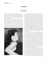
John RadovichApril I, 1921-June 27, 1981On Saturday, June 27, 1981, fishery science lostJohn Radovich, who died of a heart attack whileplaying tennis. He was 60 years old.John Radovich’s involvement with the sea beganwhile he was in the U.S. Navy (1943-46), where hebecame a diver. After the war, he graduated from theUniversity of Southern California with a degree inzoology. He later obtained a master’s degree in publicadministration at Sacramento State University, and atthe time of his death was in the latter stages of worktoward a Ph.D. degree at University of California,Davis.In 1949, John joined the California Department ofFish and Game as a seismic observer, and later becameaffiliated with the Sea Survey Project. He becameAssistant Director of the California StateFisheries Laboratory at Terminal Island, spent 1955 inSacramento as Assistant Marine Resources BranchChief, and in 1956 became leader of the PelagicFisheries Investigations at Terminal Island. In 1963 hebecame Chief of Marine Resources Branch in Sacramento.Operations Resource Branch was created in1969 with John at its helm. In 1979 he was appointedSenior Marine Advisor to the Director of the CaliforniaDepartment of Fish and Game.Radovich was involved with a number of professional,scientific, and fishery management organizationsand committees. He was a member of the AmericanInstitute of Fishery Research Biologists and, at thetime of his death, president. He was a member of theAmerican Fisheries Society and Pacific FisheriesBiologists, as well as a Research Associate inOceanography, Marine Life Research Group, ScrippsInstitution of Oceanography. He served on a numberof advisory committees dealing with living marine resourcesresearch. John was a member of the Scientificand Statistical Committee of the Pacific FisheriesManagement Council and was chairman of this committeeat the time of his death. John was deeply involvedwith CalCOFI from its inception, and was amember of the CalCOFI Committee from 1957 to1963 and from 1975 to the time of his death. Over theyears, his influence and guidance helped mold Cal-COFI policies and research activities.John’s numerous papers and publications concerningfisheries, population dynamics, and biologicaloceanography are a matter of record and need not beenumerated here.John Radovich and sea survey equipment, 1950.I knew John as a supervisor, a colleague, andmostof all-as a friend. He was a many-faceted individual.He had numerous interests, all of which hepursued with vigor. He was a yachtsman and a recreationalfisherman. As a sports fan he was unsurpassed,especially with respect to USC. He was very competitiveat tennis, both on and off the court, where heenthusiastically discussed previous or future matches.At conferences, workshops, or meetings, John’senergy was very evident-be it during the meeting,while dining, in after-meeting scientific or philosophicaldiscussions, or in recreational activities. His enthusiasmwas infectious; what might start out as arather routine discussion of a research project or proposalproblem would end up with John eagerly suggestingpossible approaches or solutions.John was a gourmet, a cook, and really enjoyedboth consuming and talking about fine foods andwines. He liked fine art and enjoyed viewing it. Infact, most activities in which John participated wereapproached with keen interest, warmth, and deterrnination.John Radovich-scientist, colleague, and friend-will remain deeply impressed in our memories. Tohis wife, Marie, and his sons, Bob and Don, I expressour deep sympathy. It is with both sadness and honorthat we dedicate this volume to him.Herbert W. Frey5

REPORT OF THE CalCOFI COMMITTEECalCOFI Rep., Vol. XXIII, 1982Part IREPORTS, REVIEW, AND PUBLICATIONSREPORT OF THE CALCOFI COMMllTEE FOR 1981With deep regret the CalCOFI Committee reportsthe loss of committee member and long-time friendJohn Radovich of the California Department of Fishand Game. The committee respectfully dedicates thisvolume of the Reports to John, who gave himself unstintinglyto CalCOFI during its formative years. Wehave asked new member Herbert Frey to write amemorial to John; it appears on the preceding page.The year was one of continued evolution in Californiafisheries and marine science, and CalCOFI memberswere active in the scientific aspects of managementas well as in studying the ecology of theCalifornia Current. A major CalCOFI cruise year(seven cruises) was completed with the WV DavidStarr Jordan (NMFS) and the WV New Horizon(SIO), featuring the introduction of a new anchovybiomass assessment technique necessitating nearly athousand vertical plankton tows for anchovy eggs andearly larvae. The “egg production method,” as thisnew technique is called, also required samplingspawning females by trawl. This was accomplished bythe combined efforts of the Jordan and a vessel charteredby the California Department of Fish and Game.Recognizing the potential widespread use of this newtechnique, the Coastal Division of the SouthwestFisheries Center is preparing a handbook on its useand interpretation. During the 1981 cruise year, theegg production method was calibrated with the larvalcensus method, and the results were presented to thePacific Fishery Management Council. This year theCalCOFI cruises added four 48-hour stations, whoseobjectives were to relate the larger-scale patterns ofchlorophyll, productivity, and zooplankton biomass tophysical structure and to compare patchiness of biologicalfeatures on large and small scales.The CalCOFI Conference this year was held at theUniversity of Southern California’s Idyllwild ConferenceCenter and featured the symposium “Reminiscencesof California Fishery Research and Manage-ment. ” Besides the six symposium papers reprinted inthis volume, forty-three additional papers were presented.A round table discussion on the state ofCalifornia fisheries was chaired by Herbert Frey ofCalifornia Department of Fish and Game. A plenarysession with the Eastern Pacific Oceanic Conference(EPOC) highlighted the last day of the meeting; Cal-COFI Coordinator Reuben Lasker presented an overviewof present and future CalCOFI activities toEPOC participants.The CalCOFI committee has continued to pursue anintrospective course in this year of shrinking budgetsand greater demand for resources. The future of Cal-COFI continues to be of concern. Thus letters weresent to a large list of “friends of CalCOFI” solicitingtheir comments on what they think the future activitiesof CalCOFI should be. Almost a hundred correspondentsreplied, and we are in the process of consideringeach suggestion.In 1981 we published CalCOFI Atlas No. 29: Teleconnectionsof 700 mb Height Anomalies for theNorthern Hemisphere, by Jerome Namias. No. 30 ishaving its final artist’s review at this writing; it isVertical and Horizontal Distribution of SeasonalMean Temperature, Salinity, Sigma-t, Stability,Dynamic Height, Oxygen and Oxygen Saturation,1950-1 978 in the California Current, by RonaldLynn, Kenneth Bliss, and Lawrence Eber of theSouthwest Fisheries Center. Abraham Fleminger is theeditor of the Atlas series.The reviewers and editorial staff of this volume,particularly Julie Olfe, are to be congratulated for theirexcellent work.The CalCOFI CommitteeIzadore BarrettHerbert FreyJoseph Reid7

FISHERIES REVIEW: 1980 and 1981CalCOFI Rep., Vol. XXIII, 1982TABLE 1Landings of Pelagic Wet Fishes in California in Short Tons in 1964-81Pacific Northern Pacific Jack Pacific MarketYear sardine anchovy mackerel mackerel herring squid Total1964 6,569 2,488 13,414 44,846 175 8,217 75,7091965 962 2,866 3,525 33,333 258 9,310 50,2541966 439 31,140 2,315 20,431 121 9,512 63,9581967 74 34,805 583 19,090 136 9,801 64,4891968 62 15,538 1,567 27,834 179 12,466 57,6461969 53 67,639 1,179 26,961 85 10,390 105,3071970 22 1 96,243 311 23,873 158 12,295 133,1011971 149 44,853 78 29,941 120 15,756 90,9471972 186 69,101 54 25,559 63 10,303 104,9931973 76 132,636 28 10,308 1,410 6,031 150,4891974 7 82,691 67 12,729 2,630 14,452 112,5761975 3 158,510 144 18,390 1,217 11,811 190,0751976 27 124,919 328 22,274 2,410 10,153 160,1151977 6 111,477 5,975 50,163 5,827 14,122 187,5701978* 5 12,607 12,540 34,456 4,930 18,898 83,4361979* 17 52,768 29,392 17,562 4,651 18,954 123,4341980* 38 46,873 32,349 22.225 7,109 16,021 124,6151981* 31 57,355 42,477 15,513 6,444 24,840 146,660*Preliminaryem Area. During 1980 the price for anchovy rangedfrom $49-$56 per ton in southern California.Sampling indicated the age composition of anchoviestaken by the Southern Area spring fishery was94% 1979 and 1978 year-class fish, with very fewolder fish.During 1980 an estimated 4,600 tons of anchovieswere used for live bait and 1,300 tons for other nonreductionpurposes.Calendar year 198 1 began with approximately18,000 tons of the 1980-81 season quota having beentaken.Monterey area boats did not actively fish for anchoviesuntil April. In early May effort toward anchoviesstopped for the remainder of the season whenmarket squid appeared in Monterey Bay, and thismore lucrative fishery began.The season closed with 4,736 tons (Table 2) havingbeen landed in the Northern Area.In the Southern Area the wetfish fleet began fishingimmediately after the holiday season. With a price of$60.50 per ton, interest was high; some 27,000 tons ofanchovies were landed prior to the February-Marchclosure.When the season resumed on April 1 , fishing effortonce again was brisk, even though the price had fallento $55 per ton. Landings averaged 3,000 to 6,000 tonsper week into May. As the landings approached theSouthern Area reduction processing quota, on May 26the California Fish and Game Commission authorizedthe California Department of Fish and Game to increasethis quota to 90,000 tons, if necessary. Thisaction was never taken, since landings dropped offdramatically the second week of June. Anchovy re-TABLE 2Anchovy Landings for Reduction in the Southern and NorthernAreas from 1966 to 1981, in Short TonsSouthern NorthernSeason Area Area Total1966-67 . . . .. ... , .. . . . . . 29,5891967-68 ................ 8521968-69 . . .. . . . . .. .. . .. . 25,3141969-70 . . . . . . . . . .. . . .. . 81,4531970-71 . . . . . . . . . . . . . . . . 80,0951971-72 . . . . . . . . . . . . . . . . 52,0521972-73 . . . . . . . . . . . . . . . . 73,1671973-74 . . . . . . . . . . . . . . . . 109,207197475 ................ 109,9181975-76 ___._........... 135,6191976-77 . . . . . .. .. .. . . . . 101,4341977-78 . . . . . . . . .... . .. . 68,4761978-79 . . . . . . . . . . . . . . . . 52,6961979-80* . . . . . . . . . . . . . . . 33,3831980-81* . . . . . . . . . . . . . . . 62,161*Preliminary8,021 37,6105,651 6,5032,736 28,0502,020 83,473657 80,7521,314 53,4262,352 75,51911,380 120,5876,669 116,5875,291 140,9065,007 106,4417,212 75,6881,174 53,8702,365 35,7484,736 66,897mained largely unavailable until the season closedJune 30 with a total catch of 62,161 tons.On July 1, the U.S. Department of Commerce establisheda reduction quota for the 1981-82 season at408,100 tons. However, the Fish and Game Commissionagain set a lower reduction processing quota at150,000 tons.In the Northern Area the season opened on August1, with Monterey fishermen showing little interest infishing for anchovies. On September 22, two boatslanded fish, and they were later joined by a third boatin November. Fishing was moderately successful, andby the end of December 3,500 tons had been landed.In the Southern Area the 1981-82 season opened onSeptember 15, but the wetfish fleet showed no interest9

FISHERIES REVIEW 1980 and 1981CalCOFI Rep., Vol. XXIII, 1982TABLE 3Permits Issued and Quotas by Gear and Area for the1979-80 Herring Roe FisheryQuotaArea Gear Permits (short tons)San Francisco Bay Gill net (odd) 109 1,500Gill net (even) 109 1,500Purse seine 27 1,500Lampara 27 1,500Tomales and Bodega bays Gill net (odd) 34 605Gill net (even) 34 605Beach seine 1 -Humboldt Bay Gill net 4 50Crescent City Gill net 3 30Total 347 7,280were exceeded in all areas except Tomales Bay, whereonly one-half the 1,210-ton quota was taken. Theplatoon system in Tomales Bay tends to keep the catchdown because the off-week platoon is unable to fishduring periods of peak spawning activity.The 1981 roe fishery catch declined for tworeasons. Herring spawned earlier in 1981, and by thetime the regular season opened on January 5, over halfthe season’s spawning had occurred. Fishing did notbegin until January 16 because fishermen went onstrike when herring prices were lowered. During thestrike the season’s largest spawn occurred simultaneouslyin Tomales and San Francisco bays. When fishingbegan after the strike, over 80% of the spawningactivity had ended in San Francisco Bay, and only onelarge spawn occurred in Tomales Bay during the remainderof the season.The herring spawning biomass was estimated in1980 and 1981 for Tomales and San Francisco bays.The Tomales Bay population was estimated at 6,023tons and 5,576 tons in 1980 and 1981. The decline in1981 reflects normal variation around a long-termaverage population size of 6,000 tons. The San FranciscoBay population estimates have increased recentlybecause of improved survey techniques, whichnow emphasize surveying subtidal rather than interdialspawning areas. San Francisco Bay spawning biomassestimates were 52,900 tons in 1980 and 65,400 tons in1981.The base price paid to fishermen peaked in 1980 at$2,000 per ton for 10% roe recovery and ranged from$1,000 to over $3,000. Gill net catches generally havea higher roe recovery than roundhaul landings.Japanese consumers balked at retail prices for herringroe that reached $60 a pound in 1980, and thebase price for herring was dropped to $1,200 per ton atthe start of the 1980 season in December. When theregular season opened in January 198 1, the base priceAreaTABLE 4Permits Issued and Quotas by Gear and Area for the1980.81 Herring Roe FisheryQuotaGear Permits (short tons)San Francisco Bay Gill net (x) 100 1,250Gill net (even) 110 1,500Gill net (odd) 110 1,500Purse seine 23 1,500Lampara 29 1.500Tomales and Bodega bays Gill net (even) 34 600Gill net (odd) 34 600Beach seine 1 -~~Humboldt Bay Gill net 4 50Crescent City Gill net 3 30Total 448 8,530for herring was dropped again to $600 per ton.Fishermen struck, and later settled on a base price of$800 per ton; this was eventually raised to $1,000 latein the season after catches declined. The roe fisherymay never be as lucrative as it once was, but pricesremain at a level where it is still a viable fishery, withan ex-vessel value of $6 million in 198 1.GroundfishCalifornia commercial and recreational fishermenlanded 45,309 tons of groundfish in 1980. Rockfish,Dover sole, and sablefish were the leading species inthe catch, with respective landings of 16,868 tons,8,538 tons, and 4,628 tons.The trawler fleet landed 36,509 tons, the majorityof the catch. Of this total, midwater trawlers landed713 tons of Pacific whiting and 4,078 tons of widowrockfish. Fishermen using line, trap, and gill netslanded an estimated 5,500 tons of groundfish. Thiscatch was predominated by rockfish and sablefish.Recreational fishermen caught an estimated total of3,300 tons of groundfish, most of which wererockfish.The 1980 landings were the result of increased effortby a larger fleet. Significant events in 1980 werethe further development of the midwater trawl fisheryand the decline in the trap fishery for sablefish.Groundfish landings continued to increase in 198 1.Landings by commercial and recreational fishermenwere 48,797 tons. The major species in the catch wereseveral species of rockfish (20,710 tons), Dover sole(10,143 tons), and sablefish (7,283 tons). Otherflounders, lingcod, and Pacific whiting were also importantin the catch.The trawler fleet increased to 193 vessels; the additionswere new, larger, more mobile vessels, andmany were from Oregon or Washington.12

FISHERIES REVIEW 1980 and 198 1CalCOFl Rep., Vol. XXIII, 1982The midwater trawl fishery for widow rockfish expandedin 198 1. The fleet extended its operations fromoff Eureka to the San Francisco area. The annual catchof widow rockfish was 4,129 tons. The Pacific whitingcatch declined to 2,674 tons concurrent with theincrease in widow rockfish.Sablefish landings increased to 7,283 tons, ascatches by all gears increased.The increasing trend of the groundfish fishery continued.Innovative harvesting, processing, and marketingtechnology contributed to its development.Groundfish continued to be important to recreationalfishermen. Rockfish and lingcod were the majorspecies in the recreational catch.Dungeness CrabStatewide landings of Dungeness crab (Cancermagister) totalled 13.6 million pounds during the1979-80 season, compared to 8.3 million poundslanded during the 1978-79 season.Landings for Crescent City, Trinidad, Eureka, andFort Bragg were 5.7, 1.1, 5.5, and 0.7 millionpounds , respectively. The northern California seasonopened December 1, 1979, but price disputes slowedeffort until December 13, when a price of 509 perpound was agreed upon. On February 5, 1980, theprice jumped to 759 and remained at that level the restof the season. Crab condition at the start of the seasonwas good, and 85% of the season’s catch came acrossthe docks by the end of January. Only 46,000 poundswere landed during the season extension from July 16to August 3 1. Approximately 380 vessels engaged inthe north coast fishery.San Francisco area landings totalled 633,000pounds. The 1979-80 season opened on the secondTuesday in November, and price was settled the sameday at $1.05 per pound. In December the pricedropped to 609 but climbed back to $1.15 by the endof the season. Only 2,700 pounds were landed duringthe season extension from July 1 to 31. The seasonextension excluded the Bodega Bay area where softand filling crabs were dominant during May and June.Landings in the Monterey and Morro Bay areas totalledonly 1 1,500 pounds.The statewide Dungeness crab landings during the1980-81 season totalled 12.0 million pounds.In northern California, total landings for CrescentCity, Trinidad, Eureka, and Fort Bragg were 6.4, 0.8,3.3, and 1 .O million pounds, respectively. The seasonopened December 1, but gear was not set until December2, when fishermen agreed to 599 per pound.Exceptionally good weather and open markets contributedto record landings of 8.2 million pounds duringDecember. The previous high for any monthlyperiod was 7.3 million pounds landed during December1977. The price jumped to 75Q in January,$1 .OO in February, and leveled out at $1.25 in March.Only 1,600 pounds were landed during the season extensionfrom July 15 to August 3 1. Approximately 400boats participated in the fishery.The central California fishery opened the secondTuesday of November, and fishermen received $1.10per pound for crab. The price dropped to 68Q when thenorthern California season opened, but reached $1.30in February and remained there to the end of the season.Total landings for the San Francisco area were515,000 pounds. Only 6,000 pounds were landed inthe Monterey-Morro Bay areas.Pelagic Shark and SwordfishThe number of vessels engaged in the drift gill netfishery for shark grew rapidly in 1980 to 116 from30-40 the previous year. As a result, total shark landingsin southern California climbed from 2.3 millionpounds in 1979 to 3.2 million pounds in 1980. Peakshark catches occurred in August and September.The composition of the catch was 58% threshershark, 10% swordfish, 3% bonito shark, and 29% blueshark. The blue shark catch prompted most drift gillnetters to increase mesh size of their nets: some to aslarge as 20 inches stretched mesh, from an initial sizeof only 8 inches. The most popular sizes appear to be14 and 16 inches.Harpoon swordfish landings reached 1.2 millionpounds in 1980, about one-third higher than the previous1 O-year average.Harpoon success, which is associated with the“finning” behavior of swordfish, was greatest duringthe months of July through November, with peak successin September.Gill net swordfish landings occurred somewhatlater, with peak success in November. Prior to the driftgill net fishery, it had been assumed that whenswordfish were no longer seen “finning,” they hadleft local waters. It now appears that swordfish mayremain in local waters in large numbers as much as 2months longer than was previously believed.In September 1980 California Assembly Bill 2564passed, restricting the number of drift gill net permitsthat could be issued. By the end of the 1981 fishingseason 150 vessels had participated in this fishery.Shark landings declined in 1981. The southernCalifornia season total amounted to 1.9 millionpounds. The season looked promising in April throughJune, with a good showing of fish; however, beginningin July catches slowed to the point where mostboats discontinued fishing.Very few fish “finned” for the harpoon fleet in13

FISHERIES REVIEW 1980 and 1981CalCOFI Rep., Vol. XXIII, 19821981. There were only 2,200 swordfish harpoonedduring the entire season. If the harpoon fleet’s successwas the only indicator of seasonal abundance ofswordfish in local waters, then one might concludethat few fish migrated into California waters in 198 1.However, beginning in September, the drift gill netfleet began catching subsurface swordfish in largenumbers. By the end of October swordfish landings bydrift gill nets had exceeded the entire season harpooncatch by a factor of two. November, which normallyrepresents the peak in gill net landings, would likelyhave doubled the catch again, but the Director of theDepartment of Fish and Game closed the season inresponse to a quota established by Assembly Bill2564. This quota is based upon the success of theharpoon fishery and not upon the condition of theswordfish resource.Southern California Recreational FisheryCommercial Passenger Fishing Vessel (CPFV)anglers in southern California enjoyed good fishing forsurface species during 1980. Pacific bonito contributedheavily to landings, with over 561,000 taken.The moderately strong 1979 year class made up mostof the catch and enabled bonito landings to reach a5-year high. Fishing for kelp bass and sand bass improvedover the previous 5-year average (498,000),with 585,000 landed. Improved sand bass catcheswere responsible for most of the increase; kelp basscatches remained relatively stable. Pacific mackerellandings continued to increase from a low point of51,000 in 1976. By year’s end, they had reached1,315,000 because of large landings of 1976 and 1978year-class fish.Fishing for albacore improved from the previousyear, with 21,000 landed-double the 1979 catch.Albacore catches were depressed because of warmwater conditions, the same phenomenon that accountedfor good fishing on other surface species.Catches of two species with low population levelscontinued to decline. California barracuda landingstumbled to a 4-year low of 28,000 fish. White seabasscatches were also depressed, with 1,000 landed. Only1978 produced fewer fish for CPFV anglers. Rockfishcatches also were down in 1980, with 3,300,000landed, well below the previous year’s mean of3,700,000.Throughout the year the California Department ofFish and Game, under a contract with the NationalMarine Fisheries Service, conducted the Californiasegment of the National Marine Fisheries StatisticsSurvey. The study was designed to estimate catch andeffort for ocean anglers. Preliminary estimates ofangler effort showed there were between 8.18 and9.08 million angler-trips in southern California during1980. Catch data were not available.Partyboat anglers continued to do well as 1981turned into a near repeat of 1980. Surface fish werestill abundant, and anglers’ catches reflected that fact.Most 198 1 partyboat data have been processed and areavailable for analysis, but information for severalmonths is still unprocessed and not available in a usableform. Preliminary data from CPFV showed bonitolandings were down 20% from the previous year butwere still expected to reach 454,000. Fishing for kelpbass and sand bass improved by 21%, with the catchexpected to reach 702,000 fish. The entire increasecan be attributed to improved kelp bass landings.Landings of Pacific mackerel declined significantly,with only 1,004,000 fish taken, 21% below the 1980take. Lack of a strong incoming year class to replacethe 1976 and 1978 year classes is responsible for this.California halibut catches doubled from the previousyear, with over 13,000 expected to have beenlanded. Strict enforcement of the 22” size limit is apparentlyadding substantially to catches in the fishery.Landings of California barracuda increased dramatically,with the catch projected to reach 77,000 for theyear. Increased catches can be attributed to an influxof adult fish from Mexico, because of warm water,rather than to an increase in the local population.White seabass landings also benefited from warmwater, with an anticipated 1,600 fish taken, up 60%from the previous year.Albacore fishing improved slightly, with approximately22,000 fish landed. The season was short; mostfish were taken during July and August. Anglers whosought rockfishes were rewarded with improvedcatches. The 198 1 catch should approach the previous5-year mean of 3.7 million fish.Marlin fishing off southern California was exceptionallygood during 198 1. The season started the earlieston record (June 27) and ran through November.In total, 1,540 marlin were taken, with the month ofSeptember producing 790 fish, a normal season’scatch under average conditions. Offshore anglers alsowere rewarded with exceptional bigeye tuna fishingduring the summer. Although the number of fishlanded was small (approximately 500), their large size(50 to 250 pounds) made most fishermen happy.Dennis BedfordSteven CrookeTom JowRichard KlingbeilRobert ReadJerome SprattRonald Warner14

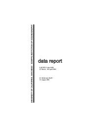
STAUFFER AND CHARTER: 1981-82 NORTHERN ANCHOVY SPAWNING BIOMASSCalCOFI Rep., Vol. XXIII, 1982THE NORTHERN ANCHOVY SPAWNING BIOMASS FOR THE 1981 -82 CALIFORNIAFISHING SEASONGARY D. STAUFFER AND RICHARD L. CHARTERNational Oceanic and Atmospheric AdministrationNational Marine Fisheries ServiceSouthwest Fisheries Center .La Jolla, California 92038ABSTRACTThe biomass of the central subpopulation of thenorthern anchovy during the 1981 spawning season isestimated to be 2,803,000 short tons, based on thelarva census method. Anchovy stock was surveyedover its geographic range on four cruises during thesix-month period from January to June. The anchovylarvae in the plankton samples were sorted, counted,and measured, and the data were summarized to formlarva census information for estimating the anchovyspawning biomass. The resulting 1981 estimate of2,803,000 tons is approximately 58 percent greaterthan the 1980 estimate of 1,775,000 tons. The optimumyield for the central subpopulation in the1981-82 fishing season is 601,000 short tons, asspecified by the yield formula given in the PacificFishery Management Council's Northern AnchovyFishery Management Plan. Within the U.S. 200-mileFishery Conservation Zone, the optimum yield is420.700 tons.RESUMENLa biomasa de la subpoblacion de Engruulis morduxdurante la temporada del desove en 1981 se calcu16ser de 2,803,000 toneladas cortas, basado en elmktodo de censo de larvas. La existencia de anchovetafue reconocida durante cuatro cruceros por toda suextension geografica, durante un period0 de seismeses entre enero y junio. Las larvas de anchoveta enlas muestras de plancton fueron separadas, contadas, ymedidas, y 10s datos fueron resumidos para formar lainformacion del censo de larvas para estimar labiomasa de desove de anchovetas. La estimacion resultantepara 1981 de 2,803,000 toneladas es aproximadamenteel 58 pOr ciento mas que la de 1980, de1,775,000 toneladas. El rendimiento optimo para lasubpoblacion central durante la temporada de pesca en1981 -82 es 601,000 toneladas cortas, especificadopor la formula de rendimiento presentada por elPacific Fishery Management Council en su Plan deAdministracion de la Pesqueria de Anchoveta delNorte. Dentro de las 200 millas que abarca la Zona deConservacion de la Pesqueria de 10s EE.UU., el rendimientooptimo es 420,700 toneladas.[Manuscnpc received February 12, 1982.1INTRODUCTIONThe harvest plan for northern anchovy, Engruulismordux, in California is specified in the PacificFishery Management Council's (PFMC) Northern AnchovyFishery Management Plan (FMP), first implementedin 1978. The optimum yield for the U.S.fishing season is set according to the optimum yieldformula given in the FMP and based on the currentestimate of the spawning biomass. The purpose of thisannual report, the fourth in a series, is to document the1981 estimate of the spawning biomass of northernanchovy for the 1981-82 California fishing season.The 1981 biomass estimate is derived by the larvacensus procedure first developed by Smith (1972) anddocumented in Appendix I of the Anchovy FMP(PFMC 1978). Stauffer and Parker (1980) later developedthe calibration for an annual larva census fromthe six-month winter-spring larva census. The 1981anchovy larva data were collected on four cruisesduring winter and spring in the 1981 CaliforniaCooperative Oceanic Fisheries Investigations (Cal-COFI) egg and larva survey. This survey was directedby the National Marine Fisheries Service, SouthwestFisheries Center (SWFC). Other agencies cooperatingin the multicruise survey were Scripps Institution ofOceanography (SIO), Instituto Nacional de Pesca,Mexico (INP), and National Ocean Survey (NOS).Samples from Mexican waters were taken by permissionof the Secretaria de Relaciones Exteriores underdiplomatic note numbers 315052, 315576, 31561 1,315984, and 316422.LARVA SURVEYThe 1981 egg and larva survey of the central subpopulationof the northern anchovy was part of the1981 triennial CalCOFI survey of the California Currentregion. The 1981 CalCOFI survey comprised sixmultiship cruises and sampled CalCOFI stations fromline 60 at 38"N off San Francisco to line 137 at 25"Noff central Baja California, Mexico, out to station90-160 to 240 nautical miles offshore (Figure 1). Tosurvey and estimate the spawning biomass of thecentral subpopulation of northern anchovies by July 1,1981, as required by the FMP, we processed andanalyzed plankton samples from only eight of thetwenty-four CalCOFI regions (4, 5, 7, 8, 9, 11, 13,15

STAUFFER AND CHARTER 1981-82 NORTHERN ANCHOVY SPAWNING BIOMASSCalCOFI Rep., Vol. XXIII, 1982L -1Figure I. CalCOFl basic station plan. The geographic range of the central subpopulation of northern anchovy is within the eight numbered regions.and 14) and from the four cruises conducted in thewinter and spring. Approximately 130 CalCOFI stationswere routinely occupied per cruise within theseeight regions. As outlined in Figure 1, these geographicregions coincide with the range of the centralsubpopulation (Vrooman et al. 1980). The four winterand spring cruises covered the major portion of theanchovy spawning season (Stauffer and Parker 1980).The anchovy survey cruises were scheduled at approximatelysix-week intervals beginning in earlyJanuary (Table 1). Each cruise was about four weekslong. The January cruise was conducted over CalCOFIlines 110 through 60 by the R/V David Starr Jordanfrom January 7 to February 1. The second cruise,TABLE 1Schedule of the 1981 Egg and Larva CruisesCruise Cruise Survey Vesselnumber month quarter name Date CalCOFI area8101 January Winter Jordan 1/7-2/1 Lines 110 to 608102 February Winter (1) Jordan 2/12-3/10 Lines llOto60withinregions 4,7,8,11,and 13(2) New Horizon 2/12-3/8 Lines 60 to I10 withinregions 5,9, and 14;lines 1 I3 to 1308104 April Spring (I) Jordan 3131.427 Lines 110 to 100 inregion 11; lines97 to 60(2) New Horizon 4/74/28 Lines 100 to 1338105 May Spring (1) Jordan 5/18-6113 Lines 90 to 110(2) New Horizon 5/19-618 Lines 87 to 6016

STAUFFER AND CHARTER 1981-82 NORTHERN ANCHOVY SPAWNING BIOMASSCalCOFl Rep., Vol. XXIII, 19828102, was run with two ships, Jordan and RIV NewHorizon, beginning February 12 and finishing March10. The cruise plan for the Jordan included an eggsurvey of CalCOFI regions 4, 7, 8, 11, and 13 toestimate the anchovy biomass by the egg productionmethod (Parker 1980). Stormy weather in Februaryprevented the ship from surveying the stations in region9 during cruise 8102. The first cruise of thespring quarter, 8104, began March 31 and ended April28. The Jordan, conducting a second egg survey inregions 7, 8, and 11, occupied inshore stations onlines 110 to 100 and all routine stations on lines 97 to60. The New Horizon surveyed the southern lines beginningwith line 100, duplicating occupancy of region11. The last cruise, 8105, began May 18 andended June 13. The Jordan surveyed from lines 90 to110, the New Horizon from lines 87 to 60.The plankton samples were collected and processedwith methods identical to the 1979 and 1980 surveysreported by Stauffer (1980) and Stauffer and Picquelle(1981). The plankton was sampled with a CalCOFIbongo net towed at a 45" angle from a maximum depthof 200 meters (Smith and Richardson 1977). Theplankton samples from the starboard half of the bongonet were sorted. All of the plankton in a sample wassorted if the station was beyond 200 miles from shoreor if the plankton volume was less than 26 ml; otherwise,a 50 percent aliquot of the sample was sorted. Inall, 534 samples were collected and processed. Nineteenstations in region 11 were occupied twice duringcruise 8104. The larva counts for these paired sampleswere averaged for the cruise. Because cruise 8105ended June 13, time was too short to sort all theplankton samples for the July 1 deadline. Therefore,samples were not sorted for the stations in region 5offshore of central California-a region with few anchovylarvae in May in the past. The larva data wereentered into the computerized CalCOFI data managementsystem where the data are edited, filed, processed,and summarized into larva census values forwinter and spring quarters.SURVEY RESULTSThe geographic distribution of anchovy larvae in1981 has expanded somewhat farther offshore comparedto the past three years. The number of larvae perstation was low in the January cruise. The number oflarvae per station in the February-March cruise increasedtenfold over the January samples. The peakoccurred in the April cruise, with the number of larvae50 percent greater than in the February-March cruise.By May-June the number of larvae per station haddecreased to a level similar to that in January. Asshown in Figure 2, larvae in northern regions 4 and 5were most abundant in the winter quarter cruises. OffBaja California, anchovy larvae were most abundantduring March and April. Few larvae were taken therein the January and June cruises. The Southern CaliforniaBight, represented by region 7, contained thelargest portion of the anchovy larvae. For the first timesince 1975, a number of anchovy larvae were found inoffshore region 9 during the April cruise. Unfortunately,stations in region 9 were not occupied duringthe February-March cruise. The large size of the larvaein region 9 suggests that the larvae were relativelyold and were probably carried offshore by the CaliforniaCurrent and upwelling plumes arising off centralCalifornia. The first major upwelling of the 1981 seasonoccurred from March 26 to April 9 off central andsouthern California (A. Bakun, Pacific EnvironmentalGroup, pers. comm.).Of the 255 stations occupied in the winter quarter,56 percent, or 143 contained anchovy larvae. For thespring quarter, 51 percent, or 134 out of 260 stationscontained anchovy larvae. The larva census compiledfor the eight regions of the central subpopulations is11,127.4 X 109 larvae for the winter quarter and14,164.3 X 109 larvae for the spring quarter. Thecombined winter-spring larva census, L ws, is25,92 1 ..7 X 109 larvae (Table 2).TABLE 2Estimated Larval Abundance (10l2 larvae) for the CentralSubpopulation from Appendix I, Table 2, FMPSpawner biomassWinterin millionsYear Winter Surine & smine Annual of short tons19511952195319541955195619571958195919601961196219631964196519661969197219751978197919801981,298,4071.2104.4695.5881.9115.9548.1146.3417.552,9924.81417.3778.94119.15515.10319.7568.21329.7546.7046.546-11.127,690,457,373,9881.7091.2064.3085.2368.1557.5476.71423.56724.81814.38322.69015.8656.53814.3354.0714.1849.124-14.164,988,8641.5835.4577.2973.11710.26213.35014.49615.0997.70628.38142.19523.32441.84530.96826.29422.54833.82510.88815.670-25.2921.841 ,1801.600 ,1565.208 ,5107.838 ,7688.618 ,8454.944 ,48511.960 1.17215.087 1.47915.440 1.51415.713 1.54011.827 1.15930.478 2.98643.407 4.25429.599 2.90147.540 4.65936.452 3.57230.594 2.99828.373 2.78136.768 3.60313.306 1.30417.580 1.723'18.110 1.775228.603 2.8033Spawner biomass in tons is calculated from annual larvae abundance;spawner biomass = 9.8 X IO-* X larvae abundance, from Smith 1972.IStauffer and Parker 1980*Stauffer 19803Stauffer and Picquelle 1981.17

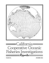
STAUFFER AND CHARTER 1981-82 NORTHERN ANCHOVY SPAWNING BIOMASSCalCOFI Rep., Vol. XXIII, 1982BIOMASS ESTIMATEThe larva census estimates of anchovy biomass forthe years 1951-69 developed by Smith (1972) arebased on annual larva census values. Stauffer andParker ( 1980) expanded the winter-spring larva censusto an annual larva census, L, with the regressionequation,L = 1.062 Lws + 1,743 X lo9.The equation is based on larva census data for195 1-75 summarized by CalCOFI regions as outlinedin Figure 1. From this equation, the 1981 annual larvacensus is 28,602.7 X lo9 larvae. The estimate ofthe 1981 spawning biomass, with Smith’s (1972)equation,B = 9.8 X 1OP8L,is 2,803,000 short tons. This is a 58 percent increaseover the 1980 estimate of 1,775,000 tons, and is thethird consecutive year with an increase in the biomassestimate since the 1978 low of 1,304,000 tons (Figure3). The 1981 larva census values for the winter andspring quarters and the resulting biomass estimate arenearly identical to survey results for 1964 and, morerecently, 1972.OPTIMUM YIELDThe optimum yield for the 1981-82 fishing seasonfor the estimated biomass of 2,803,000 tons is601,000 tons based on the formula specified in theNorthern Anchovy FMP (PFMC 1978). The optimumyield in the U.S. Fishery Conservation Zone (FCZ) is70 percent or 420,700 short tons, The U.S. capacity toprocess anchovies, including live bait, is estimated tobe 371,885 tons. The difference of 48,815 tons isavailable to joint ventures or to foreign fisheries withinthe U.S. FCZ as TALFF (Total Allowable Level ofForeign Fishing). The 1981-82 quota for the U.S.commercial fishery was set at 359,285 tons by NationalMarine Fisheries Service. However, theCalifornia Fish and Game Commission established a150,000 short-ton limit on the amount of northern anchovythat could be processed by shore-based reductionplants in California because of the discrepancybetween the 1980 estimates of biomass using the larvacensus method and the newly developed egg productionmethod (Stauffer and Picquelle 1981).ACKNOWLEDGMENTSWe thank many people for their efforts in collectingand processing the CalCOFI egg and larva data used inthis estimation. They include Scripps Institution ofOceanography (SIO) plankton sorting group, SouthwestFisheries Center CalCOFI group, and crews ofNOAA Ship WV David Starr Jordan and SI0 WVNew Horizon. We could not have accomplished thistask without everyone’s full cooperation and extraeffort.I/\ILITERATURE CITEDPacific Fishery Management Council. 1978. Northern Anchovy FisheryManagement Plan. Federal Register, 43(141), Book 2:31655-31879.Parker, K. 1980. A direct method for estimating northern anchovy, Engraulisrnordax, spawning biomass. Fish. Bull., U.S. 78:541-544.Smith, P.E. 1972. The increase in spawning biomass of northern anchovy,Engraulis rnordax. Fish. Bull., U.S. 70849-874.Smith, P.E., and S.L. Richardson. 1977. Standard techniques for pelagicfish egg and larva surveys. FA0 Fisheries Tech. Paper (175), 100 p.Stauffer, G.D. 1980. Estimate of the spawning biomass of the northernanchovy central subpopulation for the 1979-80 fishing season. Calif.Coop. Oceanic Fish. Invest. Rep. 21:17-22.Stauffer, G.D., and K.R. Parker. 1980. Estimate of the spawning biomassof the northern anchovy central subpopulation for the 1978-79 fishingseason. Calif. Coop. Oceanic Fish. Invest. Reu. 21:12-16.01 4 , I I I I I Stauffer, G.D., and- S.J. Picquelle. 1981. Esiimate of the spawning1950 1955 1960 1965 1970 1975 1980 biomass of the northern anchovy central subpopulation for the 1980-81YEARFigure 3. Estimated spawning biomass for the central subpopulation of northemanchovies, 1951-81.fishing season. Calif. Coou. Oceanic Fish. Invest. Reo. 22:8-13.Vrooman, A.M., P.A. Paloma, and J.R. Zweifel. 1980: Electophoretic,morphometric, and meristic studies of subpopulations of northern anchovy,Engraulis rnordax. Calif. Fish and Game, 67(1):39-51.19

PUBLICATIONSCalCOFI Rep., Vol. XXIII, 1982analysis for fisheries management plans. Ann Arbor SciencePublishers, Inc., Ann Arbor, Michigan.Kaupp, S.E., and J.R. Hunter. 1981. Photorepair in larval anchovy,Engraulis mordax. Photochemistry and Photobiology33:253-256.Lasker, R. 1981. Factors contributing to variable recruitment ofthe northern anchovy (Engraulis mordax) in the CaliforniaCurrent: contrasting years, 1975 through 1978. Pp. 375-388 inR. Lasker and K. Sherman (eds.), The early life history of fish:recent studies. The Second ICES Symposium, Woods Hole,2-5 April 1979. Rapp. P.-v. Kiun. Cons. Int. Explor. Mer 178,605 p.. 1981. The role of a stable ocean in larval fish survival andsubsequent recruitment. Pp. 80-87 in R. Lasker (ed.), Marinefish larvae: morphology, ecology, and relation to fisheries.Washington Sea Grant Program, Univ. Wash. Press, Seattle., ed. 1981. Marine fish larvae: morphology, ecology, andrelation to fisheries. Washington Sea Grant Program, Univ.Wash. Press, Seattle, 131 p.Lasker, R., J. Pelkz, and R.M. Laurs. 1981. The use of satelliteinfrared imagery for describing ocean processes in relation tospawning of the northern anchovy (Engraulis mordax). Rem.Sens. Environ. 11:439-453.Lasker, R., and K. Sherman, eds. 1981. The early life history offish: recent studies.The Second ICES Symposium, Woods Hole,2-5 April 1979. Rapp. P.-v. RCun. Cons. Int. Explor. Mer 178,605 p.Mais, K.F. 1981. Age-composition changes in the anchovy Engraulismordax central population. Calif. Coop. Oceanic Fish.Invest. Rep. 22:82-87.. 1981. California Department of Fish and Game assessmentof commercial fisheries resources cruises, 1980. Calif.Coop. Oceanic Fish. Invest. Data Rep. 3O:l-64.Mallicoate, D.L., and R.H. Parrish. 1981. Seasonal growth patternsof California stocks of northern anchovy, Engraulis mordax,Pacific mackerel, Scomber japonicus, and jack mackerel,Trachurus symmetricus. Calif. Coop. Oceanic Fish. Invest.Rep. 22:69-81.Methot, R.D., Jr. 1981. Spatial covariation of daily growth ratesof larval northern anchovy, Engraulis mordax, and northernlampfish, Stenobrachius leucopsarus. Pp. 424-43 1 in R.Lasker and K. Sherman (eds.), The early life history of fish:recent studies. The Second ICES Symposium, Woods Hole,2-5 April 1979. Rapp. P.-v. RCun. Cons. Int. Explor. Mer 178,605 p.Miller, D.J., and R.S. Collier. 1981. Shark attacks in Californiaand Oregon, 1926- 1979. Calif. Fish Game 67(2):76- 104.Moffatt, N.M. 1981. Survival and growth of northern anchovylarvae on low zooplankton densities as affected by the presenceof a Chlorella bloom. Pp. 475-480 in R. Lasker and K. Sherman(eds.), The early life history of fish: recent studies. TheSecond ICES Symposium, Woods Hole, 2-5 April 1979. Rapp.P.-v. RCun. Cons. Int. Explor. Mer 178, 605 p.Moser, G.H. 1981. Morphological and functional aspects ofmarine fish larvae. Pp. 90-131 in R. Lasker (ed.), Marine fishlarvae: morphology, ecology, and relation to fisheries.Washington Sea Grant Program, Univ. Wash. Press, Seattle.Moser, G.H., and J.L. Butler. 1981. Description of reared larvaeand early juveniles of the calico rockfish, Sebastes dallii. Calif.Coop. Oceanic Fish. Invest. Rep. 22238-95.O’Connell, C.P. 1981. Estimation by histological methods of thepercent of starving larvae of the northern anchovy (Engraulismordaxj in the sea. Pp. 357-360 in R. Lasker and K. Sherman(eds), The early life history of fish: recent studies. The SecondICES Symposium, Woods Hole, 2-5 April 1979. Rapp.P.-v. Riun. Cons. Int. Explor. Mer 178, 605 p.. 1981. Development of organ systems in the northern anchovy,Engraulis mordax, and other teleosts. Amer. Zool.21:429-446.Owen, R.W. 1981. Fronts and eddies in the sea: mechanisms,interactions and biological effects. In A.R. Longhurst (ed.),Analysis of marine ecosystems. Academic Press, p. 197-233.. 1981. Microscale plankton patchiness in the larval anchovyenvironment. Pp. 364-368 in R. Lasker and K. Sherman(eds.), The early life history of fish: recent studies. The SecondICES Symposium, Woods Hole, 2-5 April 1979. Rapp. P.-v.RCun. Cons. Int. Explor. Mer 178, 605 p.Parrish, R.H., C.S. Nelson, and A. Bakun. 1981. Transportmechanisms and reproductive success of fishes in the CaliforniaCurrent. Biol. Oceanogr. 1(2):175-203.Paulson, C.A., and J.J. Simpson. 1981. The temperature differenceacross the cool skin of the ocean. J. Geophys. Res.86(C11):11,044-11,054.Perry, M.J., and R.W. Eppley. 1981. Phosphate uptake byphytoplankton in the central North Pacific Ocean. Deep-seaRes. 28:39-49.Reid, J.L. 1981. Role of the southern ocean in the general circulation,EOS, Trans. Amer. Geophys. Un. 62(45):920. (Abstract). 1981. On the mid-depth circulation of the world ocean. InB.A. Warren and C.Wunsch (eds.), Evolution of physicaloceanography. MIT Press, Cambridge, Massachusetts, andLondon, p. 70- 11 1.. 1981. On the deep circulation of the Pacific Ocean. InProceedings of a Workshop on Physical Oceanography Relatedto the Subseabed Disposal of High-Level Nuclear Waste, BigSky, Montana, 14-16 January 1980, edited by Me1 G. Marietta.Albuquerque, N.M. Sandia Corp., p. 144-184.Schmitt, W.R. 1981. Ocean energy on parade. In G. L. Wick andW. R. Schmitt (eds.), Harvesting ocean energy. Unesco Press,p. 17-28.. 1981. Wind energy. In G.L. Wick and W.R. Schmitt(eds.), Harvesting ocean energy. Unesco Press, p. 149-171.Schulz-Baldes, M., and L. Cheng. 1981. Flux of radioactive cadmiumthrough the sea-skater Halobates (Heteroptera: Gerridae).Mar. Biol. 62:173-177.Shulenberger, E., and J.L. Reid. 1981. The Pacific shallow oxygenmaximum, deep chlorophyll maximum, and primary productivity,reconsidered. Deep-sea Res. 28:901-9 19.Simpson, J.J., and T.D. Dickey. 1981. The relationship betweendownward irradiance and upper ocean structure. J. Phys.Oceanogr. 11(3):309-323.. 1981. Alternative parameterizations of downward irradianceand their dynamical significance. J. Phys. Oceanogr.11(6):876- 882.Smith, P.E. 1981. Time series of anchovy larvae and juvenileabundance. P. 201 in R. Lasker and K. Sherman (eds.), Theearly life history of fish: recent studies. The Second ICES Symposium,Woods Hole, 2-5 April 1979. Rapp. P.-v. RCun.Cons. Int. Explor. Mer 178, 605 p.. 1981. Fisheries on coastal pelagic schooling fish. Pp.1-31 in R. Lasker (ed.), Marine fish larvae: morphology, ecology,and relation to fisheries. Washington Sea Grant Program,Univ. Wash. Press, Seattle.Smith, P.E., L.E. Eber, and J.R. Zweifel. 1981. Large-scale environmentalevents associated with changes in the mortality rateof the larval northern anchovy. P. 200 in R. Lasker and K.Sherman (eds.), The early life history of fish: recent studies.The Second ICES Symposium, Woods Hole, 2-5 April 1979.21

PUBLICATIONSCalCOFI Rep., Vol. XXIII, 1982Rapp. P.-v. RCun. Cons. Int. Explor. Mer 178, 605 p.Soutar, A., S.R. Johnson, T.R. Baumgartner. 1981. In search ofmodem depositional analogs to the Monterey formation. InThe Monterey formation and related siliceous rocks of California.SOC. Econ. Pal. & Min. Special Publ. Pacific Sect.,p. 123-147.Soutar, A,, S. Johnson, K. Fischer, and J. Dymond. 1981. Samplingthe sediment-water interface-evidence for an organicrichsurface layer. Fall Meeting Am. Geophys. Union (1981.(Abstract).Spencer, D.W., and A.W. Mantyla. 1981. Hydrographic, nutrientand oxygen data. In A.E. Bainbridge (ed.), GEOSECS AtlanticExpedition Atlas, Vol. 1. National Science Foundation,Washington, D.C.Spiess, F.N., K.C. Macdonald, T. Atwater, R. Ballard, A. Carranza,D. Cordoba, C. Cox, V.M. Diaz Garcia, J. Francheteau,J. Guerrero, J. Hawkins, R. Haymon, R. Hessler, T.Juteau,M. Kastner, R. Larson, B. Luyendyk, J.D. Macdougall, S.Miller, W. Normark, J. Orcutt, C. Rangin. 1980. East PacificRise: hot springs and geophysical experiments. Science207(4438): 1421 - 1433.Spratt, J.D. 1981. California grunion, Leuresthes tenuis, spawn inMonterey Bay, California. Calif. Fish Game, 67(2): 134.. 1981. Status of the Pacific herring, Clupea harenguspallasii, resource in California 1972 to 1980. Calif. Dept. FishGame, Fish Bull. (17l):l-99.Stauffer, G.D., and S.J. Picquelle. 1981. Estimate of the spawningbiomass of the northern anchovy central subpopulation forthe 1980-81 fishing season. Calif. Coop. Oceanic Fish. Invest.Rep. 22:8-13.Sunada, J.S., P.R. Kelly, I.S. Yamashita, and F. Gress. 1981.The brown pelican as a sampling instrument of age group structurein the northern anchovy population. Calif. Coop. OceanicFish. Invest. Rep. 22:65-68.Swift, J.H., and K. Aagaard. 1981. Seasonal transitions and watermass formation in the Iceland and Greenland seas. Deep-seaRes. 28(10A): 1107- 1129.Swift, J.H., and T. Takahashi. 1981. The contribution of theGreenland Sea to the deep water of the Arctic Ocean. EOS,Trans. Amer. Geophys. Un. 62(45):934. (Abstract)Theilacker, G.H. 1981. Effects of feeding history and egg size onthe morphology of jack mackerel, Trachurus symmetricus, larvae.4. 432-440 in R. Lasker and K. Sherman (eds.), Theearly life history of fish: recent studies. The Second ICES Symposium,Woods Hole, 2-5 April 1979. Rapp. P.-v. RCun.Cons. Int. Explor. Mer 178, 605 p.Vrooman, A.M., P.A. Paloma, and J.R. Zweifel. 1981. Electrophoretic,morphometric, and meristic studies of subpopulationsof northern anchovy, Engraulis mordax. Calif. Fish Game67( 1)): 39- 5 1.Webb, P.W. 1981. The effect of the bottom on the fast start offlatfish Citharichthys stigmaeus. Fish. Bull., U.S. 79(2): 271-276.Webb, P.W., and R.T. Corolla. 1981. Burst swimming performanceof northern anchovy, Engraulis mordax, larvae. Fish.Bull. U.S. 79(1):143-150.Weihs, D. 1981. Swimming of yolk-sac larval anchovy (Engraulismordax) as a respiratory mechanism. P. 327 in R. Lasker and K.Sherman (eds.), The early life history of fish: recent studies.The Second ICES Symposium, Woods Hole, 2-5 April 1979.Rapp. P.-v. Rkun. Cons. Int. Explor. Mer 178, 605 p.Weihs, D., and H.G. Moser. 1981. Stalked eyes as an adaptationtowards more efficient foraging in marine fish larvae. Bull.Mar. Sci. 31(1):31-36.Wick, G.L., and W.R. Schmitt, eds. 1981. Harvesting oceanenergy. Unesco Press, 173 p.Wilson, K.C., A.J. Meams, and J.J. Grant. 1981. Changes in kelpforests at Palos Verdes. Pp 77-91 in Coastal Water ResearchProject Biennial Report for the Years 1979-1980. SCCWRP,Long Beach, Calif. 363 p.Young, Y.D., and C.S. Cox. 1981. Electromagnetic active sourcesounding near the East Pacific Rise. Geophys. Res. Lett.8( 10): 1043- 1046.Zweifel, J.R., and P.E. Smith. 1981. Estimates of abundance andmortality of larval anchovies (1951-75): application of a newmethod. P. 248-259 in R. Lasker and K. Sherman (eds.), Theearly life history of fish: recent studies. The Second ICES Symposium,Woods Hole, 2-5 April 1979. Rapp. P.-v. Rkun.Cons. Int. Explor. Mer 178, 605 p.22

SYMPOSIUM INTRODUCTIONCalCOH Rep., Vol. XXIII, 1982Part IISYMPOSIUM OF THE CALCOFI CONFERENCEIDYLLWILD, CALIFORNIAOCTOBER 27, 1981REMINISCENCES OF CALIFORNIA FISHERYRESEARCH AND MANAGEMENTThe California Cooperative Oceanic Fisheries Investigations(CalCOFI) as an organized program is alittle over thirty years old. Yet the groundwork forCalCOFI was laid many years earlier by a group ofdedicated fishery biologists and oceanographers in theCalifornia Department of Fish and Game, the ScrippsInstitution of Oceanography, and the former Bureau ofCommercial Fisheries of the U.S. Fish and WildlifeService. The desire to know how CalCOFI came to bethe organization it is and what role it has played in thefisheries science of California prompted the CalCOFICommittee to invite a select group of people to reviewthis history in a symposium called “Reminiscences ofCalifornia Fishery Research and Management. ” Thesymposium was convened by CalCOFI CoordinatorReuben Lasker.Speaking at the symposium were Frances Clark,former director of the marine division of CaliforniaDepartment of Fish and Game; Richard Croker,former chief of the marine resources branch ofCalifornia Department of Fish and Game; John Baxter,regional manager of the Marine Resources Regionof the California Department of Fish and Game;Patricia Powell, former California Department of Fishand Game librarian; and Arthur McEvoy of North-western University, who is studying the history ofCalifornia fisheries. Another speaker, and also thechairman of the proceedings, was Joseph Reid, ocean-.ographer and director of the Marine Life ResearchGroup at the Scripps Institution of Oceanography.The CalCOFI Committee recorded the talks given atthis symposium; the tapes were transcribed by the RegionalOral History Office of the University ofCalifornia, Berkeley. Each paper was edited and annotatedby the speaker and appears here in its amendedversion. Arthur McEvoy chose to write and submit hisas a formal paper. The University of California’s Instituteof Marine Resources (IMR), with a grant fromthe Van Camp Foundation, provided the funds fortranscribing, editing, and typing the symposium papers.We thank Fred Spiess, director of IMR, for hishelp in this regard. We received permission from JohnWiley & Sons, publishers, to reprint the excellent1981 article by John Radovich, “The Collapse of theCalifornia Sardine Fishery. What Have We Learned?”John’s insight and knowledge of the science and politicsof this fishery add immeasurably to the historicalusefulness of this symposium collection.The CalCOFI Committee23

SYMPOSIUM INTRODUCTIONCalCOF'I Rep., VoI. XXIII, 1982Participants in the 1981 Symposium of the CalCOFl Conference are, from left to right, Joseph Reid, Richard Crdter, John Baxter, Patricia Powell, Mhur McEvoy, andFrances Clark.24

CLARK: CALIFORNIA MARINE FISHERIES INVESTIGATIONS, 19 14-39CalCOFI Rep., Vol. XXIII, 1982CALIFORNIA MARINE FISHERIES INVESTIGATIONS, 191 4-1 939FRANCES N. CLARKThese are exciting times. But also there is much inthe past, and I want to go back about sixty years. Toyou that is probably a long time; it’s just yesterdayto me.Fish and game studies in California started in 1914.At that time, there was a Fish Commission composedof five men who decided that there must be a marinefisheries investigation. So they organized a Departmentof Commercial Fisheries and named NormanBishop Scofield its administrator. The responsibilitiesof this investigation were to gather statistics, to studyfishing methods, fish processing and handling, and tolearn about fishes, their habits, how they migrated,where they appeared on the fishing grounds, whenthey spawned-just the little minor details. We’re stillstruggling !Norman Bishop Scofield, to me, was the father ofcommercial fisheries investigation in California. Hewas born in 1869 in the Midwest and had a bachelor’sdegree in biology before he came to California about1890. He was known throughout the years as N.B., sofrom now on he probably will be N.B. when I refer tohim.When N.B. came to California he registered atStanford as a graduate student, and in 1895 wasawarded a master’s degree with Stanford’s firstgraduating class. While he was a student at Stanford,he studied some of the San Francisco Bay and centralCalifornia fisheries under Dr. Charles Henry Gilbert.You people probably know that Gilbert was the manwho determined, in general, that Pacific Coast salmonreturn to spawn in the streams in which they hatched.Because of N.B.’s interests and his work as a student,he was employed by the Department of Fish andGame from 1897 to 1899. Then he dropped out of thepicture for several years. He was in the East doingsome business; I don’t know what. But Californiaseemed to be his love, and he came back and wasemployed again by the Department of Fish and Gamefrom 1908 until he retired in 1939.He was a man who had the imagination to knowwhat needed to be done, and the ability to find out howto do it and to provide the means for doing it. He tookover the direction of this new fisheries investigation in1915, supposedly to study statistics. You can’t studystatistics without information and figures. So in 1915 alaw was passed that required fish buyers to issue receipts,and that was the beginning of our figures on thecatch.By 1917 N .B. discovered that you can ’t do fisheriesinvestigations without money. California at that timesold licenses for commercial fishing, for sport fishingand for hunting. That was the department’s revenue.But more money was needed, so a law was passedrequiring the dealers to pay two-and-a-half cents perpound for all fish they bought. This, plus the sale offishing licenses, was the sole support for the Departmentof Fish and Game for quite a number of years.Nothing came from the general fund. As the yearswent by, the price per pound was increased, and moremoney came in.By this time Scofield had gotten things organized.There was a way of getting information, and there wassome money, so he looked around to find somebody todirect this new investigation. He selected WilliamFrancis Thompson, who is known to all of us for hiswork throughout the years. He had done some studieson the halibut in Washington and in the northern area,and Scofield admired his work. So Thompson washired and started at Monterey. He stayed there for ayear or two and then decided that the center ofCalifornia fisheries was going to be in southernCalifornia.Thompson employed William Lancelot Scofield,known as Lance Scofield to all of us, to study sardinesand other fisheries in the Monterey area. Thompsontransferred to southern California, where he employedElmer Higgins and a few other people and started thework in that area. Thompson and Higgins used patrolboats to try to explore some of the waters offsouthern California. Thompson mentioned in some ofhis laboratory notes that they had taken eggs that hethought might be sardines. But his chief interest in thisexploration was to try to learn about albacore. At thattime the albacore canning industry was expandingrapidly.By 1918 Thompson and Scofield realized that theinformation they were getting from the dealers andtheir receipts was not adequate. They needed moreinformation for a fisheries investigation. So they setup what we have called the pink-ticket system. It requiredthree receipts: one to the fisherman; a pink copyto Fish and Game-that’s the origin of the term “pinkticket”; and a third copy kept by the dealers.Again, I want to give a little credit to another man,H.B. Nidever. He was working for patrol, first in theSan Francisco area. There he had worked with N.B.when N.B. was first employed. Nidever had tremendousadmiration for the biologists. In fact, he had usup on a pedestal, which was not justified. But he had25

CLARK: CALIFORNIA MARINE FISHERIES INVESTIGATIONS. 1914-39CalCOFI Rep., Vol. XXIII, 1982the ability to work with people, and when he went outto arrest the fishermen, he could almost make thefishermen like him for doing it!So when Nidever and N.B. felt that we needed thisdetailed information, they drew up the plan for thepink-ticket system, which is the basis for much of thedetail that we have from our fisheries. Thus thingswere under way, going nicely. Higgins and Thompsonwere working. They also employed students for ashort time during the summer vacation and occasionallyfor longer terms.By 1920, Oscar Elton Sette was working withThompson, also Harlan Holmes, Tage Scogsberg,whom some of you probably know as the man whowas with Hopkins Marine Station doing biologicalwork in Monterey Bay for a number of years, andLance Scofield. Thompson realized then that theymust have permanent quarters, and the plan for theCalifornia State Fisheries Laboratory at Terminal Islandwas drawn up. The building was constructed andsubsequently occupied in November 192 1.Things were going along nicely, but by 1922 therewere hard times. The depression that followed theFirst World War was with us. At the same time, thecost of living was rising rapidly. Doesn’t that soundfamiliar? But the price of fish dropped rapidly. Therevenue to the California Department of Fish andGame was falling off. The fishermen weren’t fishing;they weren’t being paid; and yet the cost of living wasgoing up. The biologists just couldn’t afford to work:they weren’t paid enough.At the same time, the federal government was payingits biologists more than the California Departmentof Fish and Game was paying. So things fell off. Setteand Higgins left for the Atlantic Coast to work for thefederal government; Holmes went to Seattle to workfor the federal government; and there were very fewworking at the laboratory. That led Thompson andN.B. to realize that California was the training groundfor marine fisheries students. They took the matter upwith the federal government and got some agreement.It was decided that the government would pay part ofthe salary of a few people. I don’t know how it waspaid, how much it was, whether it was a lump sum tothe Department of Fish and Game, or whether it was apart of individual salaries. But I do know that GeorgeRounsefell and Bill Herrington worked a year or twoand then went back into federal government.Then we carry on to mid-1920, when, because theeconomy was looking up, money came in and theprogram was going along nicely. In 1924, the NorthPacific Fisheries Treaty with Japan was signed. Thenin 1926 the United States and Mexico formed an InternationalFishing Commission. I am sure that this waslargely the work of N.B. Scofield, who was made thecommission’s director. They started an investigation,and several people were employed.In 1926 Thompson went to Seattle and took over thework for the fisheries investigation with the UnitedStates and Japan. Lance Scofield, who had beenworking at Monterey, was transferred to southernCalifornia and became director of the work in California.By 1928 things were expanding. Julie Phillips wasemployed, as were Dick Croker, Don Fry, and HarryGodsil. They used the patrol boats to investigate thelocal waters and the populations of sardine, albacore,and other fish along the coast.The commission with Mexico did not prove successfuland had faded away by 1929. Some of its staffwere transferred to the California Department of Fishand Game. Among them were Bert Walford andGeraldine Conner. Walford worked with differentfisheries and did quite a bit with the barracuda. GeraldineConner had been a secretary to N.B. for manyyears, and had been the secretary for the InternationalFishing Commission. Now she took over the pinktickets, a mass of which had been collected. If abiologist wanted to learn what certain fishing boatshad caught, all he had to do was to go through thismass of tickets and try to find the boats he was interestedin.Geraldine Conner is another person for whom Ihave great admiration. Her training had been limited,yet she was the person who had the ability, when therewas a job to do, to know how to do it, and to go aheadand do it. She set up a program to sort and file the pinktickets and make their figures available with details ofboat catches and kinds of fish.That is a quick summary of the first fifteen years.We might pause a moment to consider what had beenlearned, for in the beginning practically nothing wasknown about our fisheries. A little had been learnedabout albacore. Thompson had indicated that therewas some relation between albacore catch and thetemperatures of the water. Gene Scofield, a young sonof N.B., was doing work with the patrol boat Bluefinand some of the smaller boats, and had found andidentified sardine eggs and larvae.The fishing grounds for sardines and mackerel offCalifornia had been well defined. The staff hadlearned the sizes of the fish that were being taken, thefact that spawning abundance varied from year toyear, and that there were differences in the sizes ofyear classes. They knew that fish taken on the fishinggrounds in central and southern California varied tosome extent. The time of the appearance in thefisheries varied for both sardines and albacore. Quite a26

CLARK: CALIFORNIA MARINE FISHERIES INVESTIGATIONS. 1914-39CalCOFI Rep., Vol. XXIII, 1982bit had been learned about tuna. Studies of the barracudahad been made, and of the white sea bass, thePismo clam, and several of the other fisheries alongthe coast.That takes care of the first fifteen years, and we’llstart a new decade. In 1930 the government of Canadaand the provincial government of British Columbiastarted a sardine investigation headed by John Hart,again a man of great ability. He came to California,talked with the people investigating here, and kept intouch by correspondence so that the work in Canadawas integrated with that in California.In 1931 it was realized that something must be doneabout the mass of pink tickets. Their information stillwas not being made available quickly enough. So thepunch-card system, as we called it, started up. It wasreally the beginning of computers, again a tribute toGerry Conner who started the program that developedinto a computer program; she got the machines set upto punch the records, sort them, and make all therecords available on printed copies.In 1931 the sport-fish catch records were started.The Bluefin, the patrol boat that did much of the firstoceanographic work, had explored California andMexican waters. At this time, it was discovered thatthe value of fish oil and meal was greater than thevalue of canned fish. Up to this time, California hadruled that no whole fish could be directly reduced tofish meal and oil: only the trimmings, the offal, andfish that were too crushed or too small for canning. Inaddition, the commission stated that any processorcould reduce only a certain percentage of his totalcatch. Because the demand for fish meal and oil wasso great, the processors appealed to the Department ofFish and Game and obtained a grant of 130,000 additionaltons for use in reducing whole fish into meal andoil.At this time, in order to get around the department’scontrol, two ships had been organized to go offshoreand reduce fish into meal and oil beyond the state’sjurisdiction. So the pressure for the use of sardines,especially, for fish meal and oil was becoming veryheavy. In 1933 the law restricting the amount of tonnageused for fish meal and oil was removed. Then thepressure to increase the reduction of sardines mountedrapidly.By 1933 Don Fry had found, reared, and identifiedmackerel eggs and had established knowledge aboutmackerel spawning. Compared to all of the mechanicalequipment we have now, there wasn’t much inthose days. Don reared his mackerel eggs, it’s rumored,in the home bathtub. That’s the way he wasable to keep the eggs and larvae until they reached asize large enough for them to be identified.In 1934 the Bluefin made five cruises. They were inlocal and southern California waters south to La Paz,and out to Tanner Bank. Much of this was under thedirection of Harry Godsil, but all of the otherbiologists worked at turns on these different projects.Then in 1934 Gene Scofield brought out his report thatsardine eggs and larvae were taken from San Franciscosouth to Cape San Lucas, and offshore for about ahundred miles.In 1935 the tagging of tuna was started, again underthe direction of Harry Godsil. In 1936 Fry brought outthe summary of what he had learned about the mackerelspawning. Phil Roedel was employed in 1936. In1937 sardine tagging was started off British Columbia,Washington, Oregon, and California. John Janssenwas in charge of that program. The California Departmentof Fish and Game and Scripps Institution ofOceanography had released drift bottles off southernCalifornia to learn something about the surface driftsin the area.By 1938 the sardine tagging was producing evidencethat sardines were moving up the coast as far asBritish Columbia and south to Baja California waters.The tuna and mackerel taggings were bringing goodresults. It was particularly exciting in 1938 whenabout thirty-five small sardines, thirty-four to thirtyfivemillimeters in length, were taken in an albacorestomach about thirty miles off the mouth of the ColumbiaRiver and sent to California biologists, thusproving that baby sardines at times occurred even thatfar north.The pressure to use sardines for fish meal and oilwas tremendous. The industry claimed that Californiahad no justification in trying to hold the total catchdown to a basic 200,000 tons a year. Whether that wastoo small or too large no one knew, and probably willnever know. The processors, the reduction people,were vociferous in their resistance to the CaliforniaDepartment of Fish and Game’s attempt to hold downthe catch. Very unpleasant things were said about thebiologists ’ bringing out statements and not knowingthe truth about the facts they had. They couldn’t beproved and probably never can be. The processorswere certainly far from polite in the things they said tous, and they brought pressure on the federal governmentto have somebody come and really learn somethingabout sardines! So Elton Sette transferred backto California and set up a program to study sardines.I’m sure Sette did not relish this problem. TheCalifornia biologists obviously had a very big chip ontheir shoulders. Their feelings had been seriously hurt.They resisted somebody else’s coming in and showingthem that they didn’t know anything.So there were many heated meetings. There was27

CLARK: CALIFORNIA MARINE FISHERIES INVESTIGATIONS. 1914-39CalCOFI Rep., Vol. XXIII, 1982much discussion and final realization that the thing todo was to learn to work together and fuse the twoprograms so they would not overlap, but supplementeach other. Thus with all the pangs, finally CalCOFIwas born. It rapidly became a very lusty infant.Also, in December of 1935 the N.B. Scofield researchvessel was launched. This is the only time theCalifornia Department of Fish and Game has evernamed one of its boats for anything but a fish, but itwas certainly a wonderful tribute to the work that N. B.had done. In 1939 the N.B. Scofield made six cruises,traveled 16,000 miles from northern California toCentral America, and took albacore 800 milesoffshore. In the fall of 1939 N.B. Scofield retired, andhere ends my account of the first twenty-five years offisheries investigation.* * *Question: Tell us something about what you did,Frances.Clark: I came to work for the Department of Fish andGame in 1921, shortly before the move into the StateFisheries Laboratory. I stayed through to 1922, whenpeople left because of lack of funds. I went to theUniversity of Michigan to study for my doctorateunder Alexander Ruthven and Carl Hubbs. I returnedto the California Department of Fish and Game as afisheries biologist in 1926 and continued on until Iretired in 1957.Here is a little anecdote about the beginning. I hadan A.B. in biology from Stanford but was hired as asecretary and librarian. I had a very limited knowledgeof shorthand; I knew nothing about library work. But Ifortunately found that Thompson apparently didn’tcare to dictate letters, and he asked me if I wouldrather have him dictate or write the letters myself forhim to sign. That was much more fun. For two momingsa week I went into Los Angeles to a library schooland learned the rudiments of library work, and in thatway the extensive library developed by Pat Powell gotunder way.Question: I’d like to ask you, Dr. Clark, what was thepublic’s reaction to the factory ships offshore?Clark: I have a feeling that, aside from the fisheriespeople and the industry, people didn’t pay much attention.It was not a major California problem. As youprobably know, they did pass a law that fish meal andoil processed outside of California waters could not bedelivered at California ports. This, in part, shut downthe offshore fish processing. But the thing that reallystopped it was employment. The people who wereworking on the ships offshore worked twenty-fourhours a day; the union said that they could not worklonger than eight hours a day, and the wages had to beincreased. That financially broke the reduction ships,and they had to give up.Question: Through your career did you face any discrimination?I assume at that time you were one of thefew women working in the field of fishery biology.Clark: My personal experience is not that peopledidn’t want to employ women, they just never thoughtof doing so!Blanca Rojas de Mendiola: I am from the Institutodel Mar de Perk I want to tell something about Dr.Frances Clark. She was in Peni in 1953 and in thebeginning of 1954. We learned a lot from her, and allof the people who had the opportunity to work withher at that time appreciate it.28

CROKER: CALIFORNIA FISHERIES RESEARCH, 1929-62CalCOFI Rep., Vol. XXIII, 1982AN ICONOCLAST’S VIEW OF CALIFORNIA FISHERIES RESEARCH, 1929-1 962RICHARD S. CROKERI’m going to talk about the early days of fisheriesand research in California from a somewhat differentviewpoint than anybody else, I’m sure. It just happensthat Herb Frey’s round table, giving some idea of thehazards and pitfalls of fisheries research and management,and Frances’s historical review fit in perfectly.We didn’t get together on this, but it just works outfine.In answer to some of the questions, though, aboutFrances, let’s just say that the fisheries research fieldwas exactly sixty years ahead of the Supreme Court. Ithink it’s a credit to the people in our field that we didget that head start.I’m going to talk somewhat about myself, not becauseof any egotistical trait, but because I want to putthings into perspective, and maybe you will get anidea of my philosophy. An iconoclast originally wassomebody who smashed the icons in the Russianchurches and went to jail for it. I like to smash a lot ofthings, but I never went to jail for it.But looking back, after Reuben talked me into thispresentation, I began to think that things are kind of apattern; things are kind of funny. But I might say thatall this time I have been marching to a different drumbeatthan a lot of people, except that since I married aScottish girl, let’s say that I’ve been marching to adifferent bagpipe! So three times I listened to thatinternal bagpipe and marched off.The first time, to give you a little background, Imarched off to World War 11. The bagpipes alwaysstirred me, and I envisioned myself as climbing out ofthe trenches and slaughtering the enemy. Anyway, Imarched off. 1’11 give you a little anecdote, and it’s atrue one, too. Strangely enough, I was taken in to seemy new commanding officer at my first station. Theadjutant introduced me, and the grim-visaged colonelsaid, “Major, what is his background?” The adjutantsaid, “He’s a fisheries biologist, sir.” The colonelsaid, “For Christ’s sake!” I heard him muttering,“What are we going to do with this bastard?” Then helooked at me, and said, “Lieutenant, have you evercommanded troops?” I said, “No, sir!” in my mostmilitary manner. He looked at me with that wellknownsteely eye, and with precise, grammaticalEnglish he said, “If I were to ask you this questiontwenty-four hours from now the answer would be,‘Yes, sir. ’ You are as of now in command of StudentSquadron 57. ”So from then on, his and my careers both wentrapidly downhill. Not long after, he was court-martialed for accepting bribes from civilian contractors.In disgrace, he committed suicide, and indisgrace his son had to resign from the Army.As for me, when I came back from the service, Iwas made a fisheries administrator with CaliforniaFish and Game. That was a quick step from amediocre biologist to a harassed administrator, andthat’s one step below even a lousy biologist. But Iwant to make the usual disavowal. Any remarks I maymake from now on do not reflect the views of anyagency or company for which I have worked, and mycomments have not been cleared by any of my pastbosses, one of whom was too modest to mention it toyou-Frances herself. So here we go.When I came to work, it was actually a collegevacation in 1928. In 1929 I was a full-time temporary.Like a temporary World War I1 building, a temporaryappointment in state service often becomes permanent.There weren’t very many of us, just a handful,and we all knew each other. We weren’t pioneers byany means. I’m not sure whether we were second orthird generation, but there weren’t many ahead of us,and most of them, as Frances mentioned, were thegreats who laid the groundwork of early fisheriesresearch.In the early thirties there was an extreme shortage ofqualified personnel. I was working, but I wasn’t qualified.There was a great shortage of public support,and there was a great shortage of funds. Frances alludedto the modem equipment that’s now available.You should have seen what we had. If you will look atthe pictures in that book over there, you will see HarryGodsil and me hauling a net. I’d like to tell you aboutthat day for several reasons. This was in 1934, offCoronado Strand. We were after young sardines. Theboat we had was the Bluefin, the patrol boat. We got itfor about one week a month or so, and the rest of thetime it was used to harass illegal fishermen.We also had what we called Bluefin, Jr., a skiff thatmust have weighed a ton, dead weight with nothing init. It was a homble thing, with an outboard motor thatwe had to operate in a well amidships to avoid foulingthe net as it was shot off the stem. Harry and I wentout with a four-man lampara net, and one day beforelunch the two of us made eleven sets on sardines.Now, the reason that Harry and I did it and not somebodyelse was that Harry was short, and I was tall, andour fannies fitted perfectly on the stem of this boat,one above the other! You can see it in the picture.Anyway, we made eleven sets, and we caught sar-29

CROKER: CALIFORNIA FISHERIES RESEARCH, 1929-62CalCOFI Rep., Vol. XXIII, 1982dines in every set. We took them back to the Bluefinand measured them for some reason that is nowobscure. We had lunch and then went out in the afternoonand made eleven more sets. That’s how hard wehad to work with the equipment we had. Every set wemade, while Harry laid out the net, I had to row on theone side with a great big old oar because we couldn’tmake the tight circle with the motor in the middle ofthe boat.Now, there are several significant things about this.One is that there were enough sardines this size tocatch some every time we put the net in the water inbroad daylight. There were enough sardines there tosupport a small but flourishing canning industry in SanDiego. Del Monte packed small sardines in oil, inquarter-pound cans, and the fishermen called smallsizedsardines “quarter oils. ” Del Monte used to keepthe cans a year before putting them on the market, tolet the flavor set, and those sardines were superb. Tothis day-and I have sampled every kind of sardine,everywhere in the world, I’ve only found one packthat would even compare in excellence. I encounteredthe closest thing in 1966 in Ensenada at a plant calledConservas del Pacifico, known as COPASA. Theypacked a Spanish-style sardine. The fish were caughtoff Mazatlan and shipped all the way up to Ensenadaby reefer truck. COPASA also put up the best whiteand red wine produced in Mexico-from the sameplant!Anyway, it was rather significant that that was thekind of equipment we had. Another example is thestory of Don Fry and the bathtub that Frances told.However, it was not mackerel, but lobsters he raisedin the bathtub; he and his wife had to come to ourhouse to take a bath.One time we went out on the Junior, which by nowhad an inboard motor with a big flywheel. Frances,Don Fry, and I went out to tag mackerel off the outerLong Beach breakwater. The first thing that cameright by us-of course, if they had known we wereFish and Game they would have stayed away-was apurse seiner. It swamped our engine, and there wewere stranded, and the three of us sat there. Don and Ipulled our arms off on the great flywheel. Finally,I got mad and said, “Excuse me, Frances”-or“Clarkey,” as we called her in those days. I sat up onthe bow and I cursed that engine until I was blue in theface. Then I marched back to the engine and gave itone turn and chug-chug-chug-chug. Frances said, “Inever knew that swearing was any good at all!”After we finished tagging mackerel, we had madesuch slow progress getting out there that we knew thebottom was fouled. Anyway it had been a long day,and there were no accommodations on board, so we’dgo over the side to scrape the seaweed and the growthoff the bottom. In those days one never mentionedgoing to the bathroom when in a situation like that, sowe could do it while we were scraping off the bottom.So that’s the kind of thing we had to do. One day,the fellow over at the dock where we kept this Juniorphoned me up and said, “Mr. Croker?” I said,“Yeah. ” “I’d like to tell you that the boatJunior sankat the dock.” I just said, “Good,” and hung up.That’s the kind of equipment we had to work with.This wasn’t pioneering; this was second-, thirdgenerationstuff.As I said, there was no respect for us, except amongourselves and our colleagues up and down the coast.We were sort of second-class citizens, and no one tookus at all seriously, no matter what we had to say.You’ve seen that television comedian who alwayssays, “I don’t get no respect.” Well, that was us. . . .Maybe we still don’t.We didn’t have much contact with the outside worldexcept through literature and correspondence. Francesmentioned the library, and Pat will be too modest toindicate the part it played, but it eventually became thefinest fishery library in the world. Occasionally bigshots even in those ancient days would come by, andwe’d have a little seminar. In fact, I remember oneembarrassing situation when I fell asleep during a talk.Gee, did I catch hell.There were our cruises down off the Mexican coastthat Frances mentioned and our contacts at Seattle, sowe knew that our world really extended from PugetSound to Cape San Lucas. It was kind of a parochialsituation; I guess the people in New Brunswick and inHull or Lowestoft in England were the same way.The first profound interrelationship was the sardinegroup of British Columbia, Washington, Oregon, andCalifornia. As the sardines were progressively fishedfarther north, we got together. One way or another,the laboratory and the library achieved a growing respectabroad, but still none at home. We were just likean expert: the farther from home he is, the better he israted.As Frances said, during those prewar years the statefishery laboratory was sort of a prep school for federaljobs. People just graduated and went on, and whenthey left, they always thought-I remember one ofthem telling me-that they were the top people, andthey left the scum behind. That didn’t go over verywell with us. There was-Frances alluded to it, butI’m going to talk about it-a growing rivalry betweenthe federal Fish and Wildlife Service and the threePacific states. It was not California alone. Oregon andWashington were even more bitter. We were trying todo something the federals weren’t doing, and that was30

CROKER: CALIFORNIA FISHERIES RESEARCH, 1929-62CalCOFI Rep., Vol. XXIII, 1982to conduct research and manage the fisheries at thesame time, which was quite different-as I am goingto expound upon-from just conducting research.Up until World War I1 the fish stocks, in general,were in pretty good shape. Some of the minor fisheriesneeded and received some conservation protection.We achieved quite a few things, largely through N.B.Scofield’s influence in Sacramento. He was universallyrespected, and he could get some things done.But he couldn’t buck the big canning industry. Aboutthat time, everybody was beginning to worry if thesalmon could survive both heavy fishing pressure andthe destruction of the environment. There was a greatdeal of interest in salmon at this time. But out on thecoast the sardine was king.World War I1 was an interruption in several ways,and I’ll list about four of them. First, the demand forfood caused intensification of fishing. Many of thetuna boats and the crews were drafted into the armedforces, so the tuna fishery stopped short. All of theother fisheries expanded greatly, however, to meet thedemand, and perhaps some of them kind of overdid it,as in the case of the soupfin shark, for example. Overfishingwas the name of the game. Many of thefisheries biologists and the state’s two research vesselswent off to war, leaving behind only a small, dedicatedgroup to hold the research program together.Another result of the war was that our horizons werebroadened. The biologists returned from service allover the world having seen how the rest of the worldlived and died, having observed fisheries in the field,and having met foreign scientists. It was a broadeningepisode in all our lives-traumatic, in fact. A worldwideview of the fisheries began to emerge. We beganto realize that fish were being caught everywhere andthat fish respected no national boundaries.Another result, only in California, really, was atremendous growth in population that resulted fromthe war. It was unequalled by any migration of westempeoples in historical times, 1 guess. I could see itwhile I was still in the service, even overseas. I don’tknow how many service people I met who planned tomove to California, especially Texans. I like Texasactually. It was great, no kidding! I love the Texans,too. They knew exactly how much they could take youfor, and they told you. I remember my corporal inTexas said once, “Lieutenant, don’t tell anybody, butI’m sick and tired of hillbilly music”-he played theguitar-“and I am going to throw the damn thingaway. As soon as this war is over, I’m coming toCalifornia. ” These new residents overtaxed all publicservices, causing water pollution, water shortages, destructionof aquatic habitat, and most of them fished; itall put a strain on our marine resources.After World War 11, and now we’re getting places,not only was there the broadening I just mentioned,but there also came a change in thinking. Instead ofsingle-species research, a gradual change took place,and we began to think in terms of multiple-speciesfisheries. The multidiscipline concept of the totalocean emerged; we began to think more of the wholepicture. The same occurred in game work and infreshwater work, too.One place where two disciplines got together wasfunny: we’d always laugh. We could always tell anoceanographer by his beard and, before we knew it,the biologists were wearing them, and we couldn’t tellthem apart! Even some of the oceanographers shavedtheirs off. I don’t know whether that had any meaningor not, but they did begin to work together.The several Pacific Coast agencies began to cooperateand formed the Pacific Marine Fisheries Commission.It included the states of California, Oregon, andWashington, and was approved by Congress. It waseither the first or second of the present three interstatecommissions. There are now five states in our commission.The Canadians were invited to sit in, and they contributedgreatly. The U.S. Fish and Wildlife Servicewas also an invited participant. But most of usrealized, though we never said it out loud, that theinterstate commission was in part created to keep thefeds from assuming too big a role.Incidentally, the federal agency changed its name sooften that I can’t keep track of it. But we’ll call themthe feds and, a sort of pejorative, 10s federales. Thoseof you from Mexico, particularly, will know how esteemed10s federales were !Back to the Pacific Marine Commission: at first thecommission was- heavily involved with sardines. Thatdidn’t last long because the fisheries progressivelycollapsed from north to south: B.C., Washington,Oregon, California. Then emphasis shifted to fisheriesstill of mutual concern to the three states andB.C.-the Dungeness crab, the albacore, the bottomfisheries, shrimps, and so on. But from the beginning,really, salmon was the big deal, and the federal salmonprogram became closely integrated with stateprograms. Instead of being kept out, the federal peoplewere brought in, and a marvelous working relationshipdeveloped.In California, everyone began to wonder if the sardinesupply really was inexhaustible. Some peoplewere genuinely concerned, but many in the industryrefused to worry. They were making big money andcouldn’t care less about the future. Others wanted tostay in business, and they just desired to learn if thecollapse was temporary, what caused it, and what, if31

CROKER CALIFORNIA FISHERIES RESEARCH, 1929-62CalCOFI Rep., Vol. XXIII, 1982anything, could be done to bring back the sardines.Eveything you can imagine was blamed, including thescientists, ocean currents, water temperature, sealions, offshore oil exploration, and all sorts of flightsof fancy. But nobody would even dream of saying outloud that it might be heavy fishing, because depletionwas a dirty word.After countless meetings of everyone involved, theMarine Research Committee was formed. The industryproposed it and funded it, and for thirty years youmight say the industry has been the sponsor of aworld-acclaimed ocean research program.We all entered into the new concept with disparatemotives and mixed emotions, but there was always asurprisingly good program even if it didn’t save thesardine fishery or bring back the sardine. In fact, anunderlying reason that it was started was to discreditthose fishery scientists whose studies had led themto believe that the resource could and should besafeguarded by imposing moderate restraints on overfishing.Meanwhile, a number of us went abroad to see howforeign fisheries were operated and to help the developingcountries manage their fisheries. It becamealmost unwritten policy to hire scientists who had hadoverseas service, or to grant leaves of absence so thatresearchers could get the experience that overseaswork involved.Now, let’s list the participating agencies. The severalagencies that were brought together and literallyforced to cooperate, kicking and screaming, had differentviewpoints and responsibilities that were boundto result in friction. It was indeed remarkable that theirresearch staffs could swallow their pride and subordinatetheir feelings to work together.First was California Fish and Game: this agencyhad, and still has, a dual responsibility under statelaw, as Miss Clark stated, to study all aspects of thestate fisheries and recommend appropriate conservationmeasures even if the state legislature is under nomandate to heed any such recommendations. Statescientists accepted the new setup as a slap in the face,as it was intended to be, and kept right on working.Very little of Marine Research Committee funds everfiltered down to California Fish and Game because,after all, if the sardines disappear, it’s the fault ofCalifornia Fish and Game.Personally, a second drumbeat sounded when Icame back and took an administrative job. I heard thebagpipes. When I signed on back there, like the airtraffic controllers, I had to take an oath to do my job,and that job was to save the fishery resources. I didn’t,and that made a profound impression on me. If Isometimes sound a little bitter, I am, because Icouldn’t find any way to save the sardine resourcefrom disappearing. Maybe nobody could anyway. Itook it personally and waited for the next bagpipe.The second agency was the federal Fisheries Service,which, as I said, we called Zos federules. Thisstaff had no management responsibility or expertise.Remember now, the Fish and Wildlife Service didn’tmanage or regulate any fishery except in Alaska, andthe less said about their efforts up there the better!(Not that the state of Alaska has done too much better.)I mean the Fish and Wildlife Service just wasn’tset up for managerial responsibility. They were responsibleto no one for anything except their conductof research, at which they were and still are goodbetterthan good. If the sardines disappear, too bad,but the research was good, and this was a great way toget a foothold in California anyway.The third participant was the university and academygroup-Hopkins Marine Station, Cal Academy,and Scripps. Their staffs conducted pure research onthe fish and the ocean, and this was a good way to getoutside funds, which were indeed put to good use.Their research was and is of top quality. We must notethat one agency was included largely so its very wiseand diplomatic director could act as an arbitrator andpeacemaker among the big three. Now I’d like to expressmy thanks to Bob Miller for a job done wellabove and beyond the call of duty, and for keeping thebrass working together.There came a change in attitudes toward Fish andGame biologists. I’m speaking of the working stiffs.As a result of the long, drawn-out death agonies of thesardine fisheries, there was a great change in the relationshipbetween the staff of Fish and Game and itsconstituents-the fishing industry and the sportsfishermen. After all is said and done, these two groupspaid the salaries of the state biologists through varioususer fees, so how the fishing public perceived thestaff, no matter right or wrong, is important to allconcerned.In general, before World War I1 the biologists weremore or less tolerated with amusement. We liked ourcustomers, and they sort of liked us. We were welcomein each other’s homes and on their fishing boats.The legislature rather ignored us, but our bossespushed through much useful conservation legislationwith respect to several minor fisheries-those inwhich the participants didn’t have much politicalclout. Many of these fisheries, including the salmonand trawl fisheries, whose fishermen actually askedfor more restrictions, continued to fare well.I would like to put in a word for fishermen. I saidthat we liked them and they liked us. I can honestlysay now I don’t think there is any greater bunch of32

CROKER: CALIFORNIA FISHERIES RESEARCH, 1929-62CalCOFI Rep., Vol. XXIII, 1982people to work with, whether you are for them oragainst them, than fishermen-sport fishermen orcommercial fishermen, and the fish packers and dealersand the whole rigmarole. I have worked with thesepeople literally all over the world, and there are nopeople like fishermen. You can make friends withthem, you can empathize with them, and sympathizewith them, and they with you, I think. To reiteratemore or less what the people up here said earlier,we’re working with people, not fish. If you are inmanagement research, and I think maybe ivory towerresearch, too, there are people involved. You run intopeople as you go along, and you have great timesahead of you working with the fishing industry and thesports fishermen.I remember once when there was some kind of hassleup in the legislature, and the then assemblymanfrom San Pedro, good old Vince Thomas, had a brightidea. He invited the assembly committee to go out on aFish and Game boat and observe a commercial fishingboat in action. So special permission was granted to apurse seiner to set a net in a closed area in Catalinabecause it would be calm and the legislators wouldn’tget seasick. The fishermen chose a crew composedentirely of old captains, all Yugoslav and Italian boatcaptains. So when they set the net, I could see howincompetent we were. They could do everything rightwhen it came to locating the fish and starting the set,but, boy, when they started to haul them in, theyweren’t as good as their crewmen.But anyway, the assemblymen and assemblywomenthat were there were very impressed by the rapport thatexisted between our patrol, enforcement, and researchpersonnel and the fishermen. Some of our people,both on enforcement and research, had taken the troubleto learn enough Serbo-Croatian to talk with theYugoslav fishermen and enough Italian or Sicilian totalk with the Italian fishermen. We went aboard eachother’s ships, the purse seiner and the Scofield, or itmight have been the Yellowfin. We ate in the galleysof the fishermen and on our boat. The legislators wereimpressed with that rapport, even though we were onopposite sides during some squabbles. I think that’simportant, and you all have a great opportunity tomake real friends. Some of them are miserable rascalsand, you can imagine, crooks. But they were greatguys!I met a man from the Better Business Bureau oncewho said that the most charming people he ever metwere bunco artists. And some of the fish canners were.So there was a friendly feeling at first, and it persistedon a personal basis. But as the sardine industry faltered,attitudes changed. The state biologists steppedup their talk about the need for catch restrictions,based on what seemed to them to be a classic andactual drop in sardine abundance.This was threatening to the sardine industry. If therecommendations were put into effect, their moneymakingmachine would have to slow down. Theindustry took various delaying actions. One was toconvince the legislature that the scarcity was temporary.Another was to fish even harder, following theold Japanese theory of conservation, which is “wiseuse” interpreted as “catch the fish before someoneelse does.” We call it the Alaska ethic. If it moves,shoot it or catch it. If it doesn’t move, chop it down ordig it up! Since the new administration came toWashington, we call it the James Watt syndrome.The crowning success of the sardine industry was tobring in outside scientists who might, just might, endorsethe theory that ocean fisheries are inexhaustible.To cloud the picture and cast doubt on the managementbiologists, the Marine Research Committee wasestablished. It was founded on the premise that researchshould be stepped up and carried on until thesardine is wiped out, no matter what wipes it out, andby then no one would care.In any event, the research goes on, and now we’rein a peculiar position. Herb Frey mentioned to me thismorning that if the sardines did reappear, the industrywouldn’t know what to do with them. They’ve losttheir markets; the fish would just be a nuisance. Thereare lines set up for mackerel and tuna, mostly tuna,and maybe if the sardines came back, nobody wouldreally care except the sport fishermen and the baithaulers.Meanwhile, the Department of Fish and Game’sother customers-the sport and commercial fishermenwho fish for the predatory fish that depend on sardinesfor food-were screaming at the department for notdoing something to save the sardines. Right or wrong,those fishermen were convinced that the purse seinefleet was destroying the sardine resource, not to mentionthe mackerel.This morning Paul Smith mentioned something Ihad completely forgotten: that there was once an initiativemeasure on the ballot to prohibit all purseseining south of central California, and it won a millionyes votes. A million out of three million voterswanted to do away with purse seiners altogether. Sothere was some very large public appreciation of trouble,trouble, trouble. The sportsmen pounded us andgave us hell for letting it happen.By now-about 1960-instead of being ignored ortolerated, the state biologists were denounced fromboth sides. It became frustrating to watch an industrydie while we continued really useful research, whichwas doomed from the start never to answer to33

CROKER: CALIFORNIA FISHERIES RESEARCH, 1929-62CalCOFI Rep., Vol. XXIII, 1982everyone’s satisfaction the simple question: wherehave the sardines gone and why?About then I heard the third skirl of the bagpipes. Ihad become aware of the world crisis in resources andenvironment, and world hunger and shortage of water,and all those things. I marched off again to try to dosomething, and I found I couldn’t even lick that. Sofinally I gave up. I said to hell with it and I’ll gofishing!* * *Question: What was the role that Wib Chapmanplayed in the organization of the association betweenthe feds and the state and the academic people?Croker: You’re asking a complex question about avery complex person: a man of vision, one of my bestfriends, the man with whom I have disagreed morethan anyone else. As far as I know, at least in hisproductive years, he never worked for the feds or theFish and Wildlife people. He never worked for CalFish and Game. In fact, he was at the Academy ofSciences in San Francisco and later was to become thefisheries honcho, head man in the U.S. Department ofState. He left State and turned it over to Bill Herrington,who also got his schooling in San Pedro, rightnear the lab. Then Wib went to work for the tunapeople. It was while he was with the Academy that hehelped bring the various agencies together.I remember one enlightening conversation I hadwith him during his tuna industry days. He was beingvery antagonistic toward what he called, in his inimitableway, our parochialism. He spoke in lofty termsof five hundred, a thousand million tons, and how theworld is full of fish, and people have got to eat, andwe in California were so parochial.Then I said to him, “Wib, remember, as you streamaround the world writing your wonderful long lettersand flying on exotic airlines, you’re in the jet set, andhere I am, stuck in California. I too spend time in thejet set, but mostly I am in the DC-3 set. I have to takecare of the salmon and the shrimp and the crab and thesport fisherman and all the nitty gritty. I just can’tafford to spend all of my time in a 707 or a DC-8 likeyou can.” Wib realized what I meant, that he couldtake care of the big world picture without being on thefiring line, while my staff and I had to stay home andfight the local wars. He thought about it for a while,and we saw eye-to-eye from that time on. But I nevercould swallow his idea that the total supply of all kindsof fish in the world was inexhaustible, and we couldexpand world fisheries ad infinitum. There we had todisagree.From the time we had this little conversation, he dideverything in his power to bring all the agencies closertogether. He was not a disruptive factor as far as I wasconcerned.Clark: Although my answer was, no, Wib Chapmannever worked with us, many times he did workfor us,and in his wonderful way he did a great deal for us.Question: Is this Gilbert whose name came up todaythe same one who conducted the Philippine fish survey?Croker: Yes. Several people pioneered ichthyologicalresearch and laid the groundwork for Carl Hubbs tocarry on for so long; they were Gilbert, Evermann,Jordan, and, a little bit later, Snyder. Snyder once toldme about a trip to Kodiak or somewhere where thecrew kept drinking all of his alcohol for preservingspecimens. So he put some formaldehyde in the alcoholand put a big sign on it that said, “I have addedformaldehyde; it will poison you, ” and the entire crewgot sick!I remember a scientist from Montana who was, Ithink, with Gilbert during early work in the Philippines.He got so seasick that when they put ashore, hesomehow got home-I don’t know how-and henever again left Montana. He gave up fisheries work!Seasick all the way to Manila. So those were thepioneering days.Question: Dick, I would be awfully disappointed ifyou didn’t tell the folks your perception of how peoplefelt about a fishery biologist back in the early years.You know what I mean.Croker: Oh, this is going to be tough on the interpreter,but I’ll give it in English. I told you that wedidn’t get no respect. That double negative is all rightin Spanish. One of our fellows received a letter fromhis mother asking, “Son, what are you doing now?”It’s alleged that he was so ashamed to admit being afishery biologist that he wrote, “Dear Mom, I am sureyou would be happy to know that I am the piano playerin a whorehouse.” Times have changed, I hope!34

BAXTER MARINE RESEARCH COMMITTEE AND CalCOFICalCOR Rep., Vol. XXIII, 1982THE ROLE OF THE MARINE RESEARCH COMMITTEE AND CalCOFlJOHN L. BAXTERI feel quite honored to be on a panel with Frances N.Clark and Richard S. Croker. Clark hired me, and atthat time she was director of the California StateFisheries Laboratory, and on a pedestal much higherthan I could reach. And Croker was the chief of thethen Marine Fisheries Branch, a very important jobindeed. So, as you can see, I feel a little bit out ofplace here, but I acknowledge that I am a secondstringer. Actually, they intended this speaker to bePhil Roedel, and that would have been much moreappropriate. I am like the baseball player who wasinserted in the eighth inning and then was pinch hit forin the ninth. So that’s a good analogy for my relationshipwith CalCOFI.My talk is titled “The Role of the Marine ResearchCommittee and CalCOFI,” and results from a lot oflibrary research that I hope will make sense to you andwill fit in with this symposium. The Marine ResearchCommittee (MRC) was established by an act of thelegislature in 1947. Croker generally covered thereasons and some of the behind-the-scenes occurrencesthat led to its establishment. The statute describedit as consisting of nine members, three ofwhom were ex ofJicio members with the same rightsand powers as the other members. The three were thepresident of the Fish and Game Commission, theexecutive secretary of the then Division of Fish andGame and later the director of the Department of Fishand Game (DFG), and one employee of DFG designatedby the Fish and Game Commission. Thismember was, from the very start, Dick Croker. Of theother six members, at least five were to be experiencedin and actively engaged in the canning or reduction ofCalifornia sardines.Members served without compensation. An addedtax of fifty cents per ton or a fraction of each ton ofsardines purchased, received, or taken was leviedagainst the industry. That money was put into the Fishand Game Preservation Fund and dispersed by themajority of the Marine Research Committee solely tofinance research in developing the commercialfisheries of the Pacific Ocean and developing marineproducts susceptible to being made available toCalifornians.In 1953, this law was changed. The tax was increasedto a dollar a ton for sardines and, in addition,the dollar a ton was levied on Pacific mackerel, jackmackerel, squid, Pacific herring, and anchovies. Beginningin 1956 the membership of the committee waschanged. The three ex oficio members representingthe Fish and Game Commission and the Department ofFish and Game were replaced. The six members representingthe industry remained, but one member fromthe public at large, one from organized labor, and oneto represent organized sportsmen were added.The first meeting of MRC was held on April 28,1948, at the California Academy of Sciences (CAS) inSan Francisco. At that meeting, Julian Burnette, anold reductionist, was elected chairman of MRC, aposition he held until February of 1967, when he wasreplaced by Charles R. Carry. Julian was the onlymember who served during the entire thirty-one-yearlife of MRC. Mr. Carry continued as chairman until itsfinal meeting, which was held June 29, 1978, in LongBeach. Incidentally, Dick Croker was elected secretaryat that first meeting in 1948, and he held thatposition until 1962 when he retired. He was followedby Phil Roedel, Doyle Gates, Laura Richardson, andHerb Frey.During the thirty-one years that the MRC was inexistence, revenues collected under the special tax totaledonly $3,350,000. Of this, approximately$923,000 came from sardines, $977,000 from themackerels, $1,200,000 from anchovies, $231,000from herring, and $215,000 from the squid fishery.The largest budget ever adopted by MRC was$185,000 in 1970-71, and more than half of this wasfrom carry-over funds that hadn’t been expended earlier.This, incidentally, was during the time the anchovyfishery was growing at a pretty good rate.Of course, this money represents only a small partof the total picture. It has been estimated by many thatthe “seed money” provided by MRC was important instimulating revenues that in recent years have greatlyincreased. The CalCOFI program has been over$4,000,000 a year. That $4,000,000 per year fromother sources was all spent on things over which MRCexercised some purview.In the early years, the MRC funds ranged fromabout $65,000 to $180,000; they played a very importantpart in keeping the cooperative sardine programgoing. They assisted the U.S. Bureau of CommercialFisheries (BCF) through some tough years with itsboat schedules, and provided assistance for boat crewsfor the DFG. The majority of MRC’s monies in thefirst five years went to those kinds of programs.From 1950 through 1960, Scripps Institution ofOceanography (SIO) used from $30,000 to $70,000per year, to assist with research. It’s obvious that althoughthe budget of MRC was rather small, it helped35

BAXTER MARINE RESEARCH COMMI’lTEE AND CalCOFICalCOFI Rep., Vol. XXIII, 1982the research organizations over some tough financialtimes in the early years. In the later years, MRCserved as a rather small tail wagging a rather largedog, which the CalCOFI program has become.Also, this influential group of men, particularly theindustry representatives, played a large part in encouragingthe University of California to fund SI0 forits CalCOFI part of the program. MRC memberscould talk to the president of the University of California,and also they played a large part in the foundingof the Institute of Marine Resources (IMR). Whereasin 1949-50, MRC funding was $97,500, the threemajor agencies by that time were expending about$600,000 a year on the cooperative sardine fisheryinvestigation. Ten years later, in July of 1960, MRCwas supplying about $60,000 to Scripps, Fish andGame, and BCF, and their budgets for the programtotaled $950,000. As pointed out earlier, the CalCOFIprogram is today about $4,000,000 per year.Through the forties and fifties, the major differencesamong scientists working on sardines hinderedthe implementation of management measures. AlthoughI don’t pretend to understand the total picture,the basic difference between BCF and DFG scientistswas that BCF held that year-class size was independentof spawning-stock size. This basic disagreementwas later softened when different leadership, uponfurther examination of the data, reached a decisionmore compatible with the DFG’s views.The matter was finally put to rest by Garth Murphyin his 1966 thesis on sardine population biology. Hestated: “Thus, the long series of poor year classes(1949-1963) at small stock sizes in the face of varyingoceanic climate suggests that Marr’s conclusion thatyear-class size is independent of stock size is untenable.” Further, “it seems clear that the population wasoverfished in an economic sense, and overfished in thebiological sense, too, in that the heavy mortality inducedby the fishery removed the ‘cushion’ againstpoor spawning success provided by older fish. ”The net effect of this disagreement between majoragencies over the relation of spawning-stock size andyear-class size, in my view, continued overfishing ofsardines until they were driven to the critically lowpoint where the population is today. The first legislationrestricting the size of the sardine catch was passedin 1969. MRC at last passed a motion recommending acomplete moratorium on the take of sardines at theirSeptember 1967 meeting. This legislation wasstrengthened in 1974 by further restricting the uses ofincidentally caught sardines.Now, back to the beginnings. On May 19, 1948, theMRC met in La Jolla. At that time, Robert C. Millerwas chairman of the Technical Committee (he is theone Dick Croker referred to as having a very large partin holding this thing together in the early years). Boboutlined the following lines of research to be pursuedby the then California Cooperative Sardine ResearchProgram: (1) physical-chemical conditions in the sea;(2) organic productivity of the sea; (3) spawning survivaland recruitment of sardines; (4) availability ofthe stock to fishermen, that is, the behavior of the fishas it affects catch, abundance, distribution, and migration;(5) fishing methods in relation to availability;and (6) dynamics of the sardine population andfishery.This forerunner of the later CalCOFI program wasmade up of representatives from SIO, CAS, BCF, andDFG. The California Cooperative Sardine ResearchProgram was renamed the California CooperativeOceanic Fisheries Investigations (CalCOFI) in June of1953 to recognize the expansion of the sardine programto include work on other species. In 1952, theHopkins Marine Station of Stanford University (HMS)joined the program. In 1965 or ’66, San Diego StateCollege was included. In 1974, HMS dropped out ofthe MRC part of the program, and its work in MontereyBay was taken over by Moss Landing MarineLaboratories. From 1974 through 1977, MRC fundedphytoplankton studies by UC Santa Cruz in MontereyBay. These, then, have been the agencies that benefitedfrom MRC’s funds over the years.Informal cooperative scientific studies betweenCalCOFI and Mexican scientists were begun in the fallof 1971 and continue to this day.Much of the future course of CalCOFI was determinedin the late 1950s. At the May 3, 1957, MRCmeeting a special technical committee was appointedby the chairman to examine the objectives of Cal-COFI, to define the problems involved in attainingthese objectives, to assess progress on the solution ofproblems, and to assign priorities to the remainingproblems. This committee was affectionately knownas the Three John Committee and was made up of JohnIsaacs of SIO, John Marr of BCF, and John Radovichof DFG. Elton Sette was named as an independentscientist to serve as special advisor to the chairman ofMRC and to attend all meetings of the special technicalcommittee to offer his advice and commentswhenever he considered it necessary to expediteprogress or agreement. Jack Marr was the chairman ofthis committee.At the December meeting of MRC, the specialtechnical committee presented its report, which notedthat the research program of CalCOFI, conducted bythe five agencies under MRC, had made real contributionstoward understanding the fisheries but lackedeffective coordination. To remedy these shortcom-36

BAXTER: MARINE RESEARCH COMMITTEE AND CalCOFICalCOFI Rep., Vol. XXIII, 1982ings, the committee recommended that control of theprogram be vested in a four-person committee. Therewould be one member each from DFG, from BCF,and from SIO. Each committee member would be theperson actively directing his agency’s share of theCalCOFI program. The fourth member and chairmanwould be a full-time scientific advisor hired by theMRC for this purpose. MRC and the three majoragencies endorsed the plan, and thus was born theCalCOFI Committee.The high priorities proposed by the Three JohnCommittee were (1) to further describe and investigatethe causes of the sardine’s catastrophic decline; (2) todetermine the population subgroups and their rate ofintermixing; (3) to further study the dynamics to determinethe vital statistics of the sardine population;that is, to derive an independent measure of recruitmentand appraise the best methods for determiningthe size of the spawning stock to a degree of accuracyconsistent with other associated measures; and (4) tocomplete descriptive oceanographic studies of thegeneral circulation and of seasonal and other changes.An early objective of the California CooperativeSardine Investigation, the forerunner of CalCOFI, wasto seek out the underlying principles that governed thePacific sardine’s behavior, availability, and totalabundance. By 1960 the CalCOFI Committee formulatedslightly different objectives: to acquire knowledgeand understanding of the factors governing theabundance, distribution, and variation of the pelagicmarine fishes, emphasizing the oceanographic andbiological factors affecting the sardine and its ecologicalassociates in the California Current system. Theultimate aim of the investigation was to obtain an understandingsufficient to predict, thus permitting efficientuse of the species and perhaps manipulation ofthe population. These restated objectives formalizedsome aspects of the research that had long been recognized:(1) that no pelagic fish such as the sardine canbe studied in nature as a creature isolated from itsnatural associates, (2) that such research is ultimatelyresponsible to the needs of society, and (3) that theultimate goal of this responsibility is attaining sufficientunderstanding to guide society in using the resource.Quite a change from earlier objectives.After a year of search, Garth Murphy was selectedas coordinator in November 1958. His chief responsibilitieswere to coordinate the agency programsthrough the CalCOFI Committee and to look into thesardine problem. His studies on sardine populationdynamics culminated in a 1965 Ph.D. dissertation entitled‘‘Population Biology of the Pacific Sardine(Sardinops caerulea). ” This study showed that themaximum sustainable yield of the pre- 1949 sardinepopulation was 471,000 tons for a spawning populationsize of about 1,000,000 tons. During this periodthe catch averaged 570,000 tons. In addition, theheavy fishing left too few older individuals to cushionthe population against reproductive failure. Themaximum sustainable yield of the 1960s populationwas 57,000 tons for a population of 178,000 tons.During his work with CalCOFI, Murphy receiveddata indicating that the rise of the anchovy was apparentlyin response to an environmental void created bythe decline of the sardine. Murphy states, “If this isso, the validity of a sustainable yield of sardines canbe questioned, for the reduced sardine population requiredto generate the yield would also release resourcesto the anchovies. The subsequent increase ofthe anchovy would surely alter the parameters of thesardine population in such a way as to reduce themaximum sustainable yield. As a converse, the presentsituation is not likely to alter rapidly, even if sardinefishing is stopped, unless man or nature acts toreduce the anchovy population somewhat. It appearsthat judicious use of all ecologically similar specieswithin the trophic level offers the only hope of sustainedyield. ’ ’As a result of Murphy’s work, and that of manyothers in CalCOFI’s other agencies, the CalCOFICommittee proposed the famous anchovy experimentin March of 1964. At that time, the CalCOFI Committeewas made up of Garth Murphy, coordinator;John Isaacs from SIO; E.H. Ahlstrom from BCF, whoreplaced Marr in 1959; and Baxter, from DFG, whoreplaced Radovich in 1963.This proposal was developed considering the followingthree factors: (1) the basis for the suggestedexperiment, although the most complete everachieved, still is not precise enough to foresee exactlyhow many anchovies and sardines should ultimatelybe taken; (2) a careful stepwise approach, such as wasused in South Africa, is the only defensible experiment;and (3) there are time lags in response of sardineand anchovy populations to new factors. Their lifehistories suggest that at least three years would berequired for population responses to be detected, evenin a regime of favorable environment, and there arealso time lags in scientific analysis, especially whendealing with new problems. Thus it is necessary tocarry out measurements that can follow events closelyand that will yield results that are readily interpreted.With these three factors in mind, the approach wasdivided into three phases. The CalCOFI Committeebelieved three years was the minimum for each phase.In phase I, the objective was to initiate a conservativefishery on anchovies and reduce sardine fishing justenough to produce an observable change in the system37

BAXTER: MARINE RESEARCH COMMmEE AND CalCOFICalCOFI Rep., Vol. XXIII, 1982and just enough to improve our preliminary appraisalsof the magnitude of the anchovy resource. During thisphase, a limit of 200,000 tons should be placed on theanchovy fishery, and the sardine fishery should belimited to 10,000 tons. Percentages were also establishedfor north and south of the Baja California border.The amounts to be removed during phase 11, and theareal distribution of the limits of these species mustawait the results of phase I. We hazarded a guess atthat time that during phase I1 the anchovy quota mightbe raised about fifty percent, providing the results ofphase I are not widely different from preliminary expectations.Phase 111, we felt, couldn’t be specified at all beyondindicating its objective, which was to restore thepredecline balance between sardines and anchoviesand maximize the harvest consistent with all usesfood,recreation, and so forth.Although the great experiment really has nevercome off, as a result of CalCOFI’s and MRC’s activeparticipation in the program, the Fish and GameCommission took a big step in 1964. They changedtheir policy on allowing the reduction of anchovies,which had been banned since about 1920, and permitteda quota of 75,000 tons. Because of many restrictionsand small fishing zones, it was almost impossiblefor the fishery to really develop.A fishery has continued since, with catches of up to165,000 tons. Opposition by sportsmen and even othercommercia1 groups was so great over the years that thefishery has never operated as the “experiment” thatthe proposal called for.Anyway, shortly after receiving his Ph.D. in late1965, Murphy left CalCOFI and took a position at theUniversity of Hawaii. In fact, I am told he is the onlyperson known who went from a graduate student to afull professor and took a cut in pay! Phil Roedel, whoreally should be up here instead of me, succeededDick Croker as secretary of MRC and was named theacting coordinator after Murphy left, a position heheld until the mid-seventies. Then Marston Sargentcame on and served as the MRC coordinator frommid-1971 until his retirement in 1974. Thereafter, Iguess a number of people have served as coordinator-HerbFrey, I know, for a number of years,then George Hemingway, and now Reuben Lasker.I was asked to speak on the role of MRC and Cal-COFI, and what I have discussed is a combination oftheir roles and a history of their activities. The MarineResearch Committee was established at a time whenthe sardine fishery was showing very strong signs ofoverfishing. California Fish and Game was urgingcurtailment of the catch, and had been for a number ofyears. Others were questioning that fishing was thecause of the failure of the sardine fishery. The industryagreed to tax itself to fund needed studies. Whatstarted as a delaying tactic to avoid management resultedin a research program that has provided muchbetter understanding of the California Current system,and technological development that otherwise mightnot have been possible.Of course, we lost the sardine, and I leave it to youto decide whether it was all worth it. CalCOFI continuestoday even without MRC. Would it have gottenstarted and prospered as it has without the small startMRC provided, without the coordination made possibleby MRC, without the political clout that MRC andits members exerted, which resulted in added fundingfrom other sources for furthering the CalCOFI researchprogram? Again, you decide. Thank you.* * *Lasker: Jack, I wonder if you would consider today’svery large anchovy fishery as the experiment you weretalking about, considering that a total of 300,000 tonsof anchovy is now being taken from both sides of theborder.Baxter: I considered that, and I conveniently left itout, but, yes, I agree. Of course, it hasn’t gone on forthree years. We haven’t monitored as closely, I think,as our origial experiment envisioned. But even withthe drop in anchovy biomass on our side of the borderin recent years, the sardine has failed to reestablishitself. It makes me wonder, too, but I still think it wasworth the try.Question: Jack, may I answer Lasker’s question?The reason we can’t really come off with the experimentis that there are not enough sardines left. Rememberthat we were going to cut the harvest of thesardines to 10,OOO tons. At this time I don’t think thereare 10,000 tons or close to 10,000 tons of spawningbiomass left.Comment: It’s too small to measure by our presentmethods anyway.38

REID: AN OCEANOGRAPHER’S PERSPECTIVECalCOFI Rep., Vol. XXIII, 1982AN OCEANOGRAPHER’S PERSPECTIVEJOSEPH L. REIDI suppose it’s my turn now to add what I can aboutan oceanographer’s perspective on this system. I thinkperhaps I’d better say how I got into the trade, becauseI came in sideways and unexpectedly. I enteredScripps as a graduate student in physical oceanographyin 1948, my interest in the ocean having beenengendered by some naval service. I was a student ofWalter Munk’s for a while, but he couldn’t quite keepup with me, so I got some half-time research support,the usual kind a graduate student gets, from MarineLife Research.About 1950 or ’51 I began to attend these conferences.Well, I felt myself a very sharp young physicaloceanographer who was certain to straighten thesepeople out in a very short period of time. I could notunderstand-as you will, I think, from having heardwhat these people have said, particularly Jack Baxter-whyall of these people, the feds on one side andthe loosely called confederates on the other side, werehaving such terrible battles. I really thought they assembledannually to hear me tell them about the physicaloceanography of the California Current. It took mea while to come up to speed on this.But the format of the conference was a little differentin those days. There was a higher proportion ofbusiness discussed at that time, although the papersgiven still dominated the sessions. I would usuallygive a paper, and being very full of the kind of researchthat could be done in physical oceanography, Iwould talk for fifteen minutes or so about geomagneticelectrokinetographs (GEK’s), acceleration potential,geopotential anomalies, electromotive forces, andthings of that kind. About half-way through my talk,Frances would look at me and say, “Joe, what do youreally mean?” . . . I think it might be useful if questionsof that nature were asked more frequently in themiddle of these presentations. Of course I did havesomething to say, but I need not have said it quite inthose words. By the time I thought about it and expressedit in a more rational way, nobody had anytrouble understanding it. It really wasn’t all that complicated.In fact, I think some biologists read my papersin physical oceanography in preference to othersbecause at least they can understand what I’m saying,and if they can, they should thank Frances.Then I would finally get to the end of my spiel, andRoger Revelle would get up and say, “That’s not so. ”And I would say, “Yes, it is!” And we would argue.Here I was, the lowest graduate student on the totempole at Scripps. I don’t mean to imply that Roger wasalways wrong or always right, but in those days, itdidn’t matter at all whether Roger was right or wrong;he would win those arguments. There was just noquestion of it. I would look out into the audience, andthere would be Ahlie Ahlstrom and Dick Croker andthe like, grinning like apes at my discomfiture, ofcourse. Then as I left the stage, Frances would look atme with her kind, sweet smile and pat me on the back.Our technical director, Bob Miller, whose name hascome up before, would take me out and buy me adrink. That was, I guess, one of his job requirementsunder those circumstances, one of his many functionsto keep the place going. Then we would be ready tocontinue.What was oceanography in those days, and whatwere we doing? I suppose the state of physical oceanographyin that period-and, in fact, of oceanographyin general-could be summed up in the 1942 work ofSverdrup, Johnson, and Fleming because, of course,the war had intervened, and very little had been donein most fields of oceanography during that period. Itwas Harald Sverdrup himself who started the work inphysical oceanography here, and he was one of themajor protagonists in the proposals that got CalCOFIstarted. We began with his ideas and the people that hehad trained or had begun to train. The physical oceanographersin those days were Bob Reid and Paul Horrerand Warren Wooster, who had come a little earlierthan I had, joined shortly by Feenan Jennings. I don’tknow what you think of this motley crew, but that’swhat was assembled out at the Scripps Field Annex atPoint Loma in those days.What was there to work with? Up to that timeoceanography had been dominated almost entirely bythe work of the Scandinavians and more lately by theGermans, with some from the U.S. The work waseither large-scale exploration-the Dana expeditions,the Carnegie, the Deutschland, trying to get at thegeneral circumstances of the ocean-or of localizedbays and estuaries. Nansen had done his work on thesource waters of the North Atlantic; Brennecke hadworked on the source at the other end, in the WeddellSea; and we knew at least that the major deep watermasses of the world ocean were formed mostly in theAtlantic. But the kinds of studies that they were able tomake were limited to statements about the general circulationor the mean flow, with little time or moneyfor finer-scale work on variability.However, these people were very sharp. In fact,there is a wonderful paper by Helland-Hansen and39

REID: AN OCEANOGRAPHER’S PERSPECTIVECalCOFI Rep., Vol. XXIII, 1982Nansen in 1909. They had gone to sea making traditionalhydrographic casts, measuring what they could,and when they analyzed their data, they found notlarge-scale smooth fields but rather wobbly ones.There would be a station-to-station variation of thedepth of various isotherms. Of course, they didn’t getto sea very often, and they couldn’t repeat their measurementsas much as they liked, but they at leastthought about them and wrote about the patterns. Theydidn’t know whether the patterns represented meanflows on a smaller scale than people had supposed, orwere waves of some kind, huge solitary waves, orwere little anticyclonic and cyclonic gyres. They wereable to repeat a few of their lines here and there andfound that things changed in time as well as in space.Their work was limited by the facilities at hand, butthey did say such things as, “Gee, it looks differentfrom time to time. We really should try to augment ourwork and repeat lines whenever we can, make ourobservations as close together as possible to avoidaliasing, and whenever possible, stay in one place fora while, repeating the observation to get some feelingfor the time variation.” That was 1909. Now, thatwould have been a perfect prospectus for the AtlanticMODE operation if anyone in the MODE group hadever read the paper, but I don’t think they had.That was the background in which we were working.Some notions of the general circulation were athand in 1948 when the cruises were planned, but wehad little feeling for the kind of spacing required todefine the field of flow and patterns of the othercharacteristics, and at what intervals we would have tooccupy these stations to follow their time-fluctuations.Cruise I of MLR and CalCOFI went out in March of1949, and I was on the Horizon (the old Horizon, notthe New Horizon). We also had in that early periodsuch ships as the Paolina-T and the Crest. May I havea show of hands of people in this group who were everat sea on the Paolina-T? Bravo. Well, I don’t have totell you what she was like. She was a perfectly seaworthyvessel. She would never sink-though we kepthoping! She just didn’t care which end was up.You remember perhaps what our 1949 pattern waslike. We had about twelve lines spaced 120 miles apartgoing offshore from the west coast of North America,and the stations were spaced about forty to sixty milesapart along each line. We found out from the first fewcruises that we hadn’t done it quite right. We discoveredby our own examination, not from anyone else’ssage advice, that we would have to tighten this line ofstations and spacing in order to get what we wereafter. I think I’m talking mostly about the physicaloceanographic aspects of it, but it certainly proved tobe true, and perhaps might have been noticed evenearlier, in the egg and larva work. I’m not going tocriticize the biologists at this stage; I am sure there areenough of them to do it for each other.But this was a primitive period of physical oceanography.Out in the California Current we foundstrange shapes that did not fit any of the concepts wehad in mind. There were unexpected loops and whorlsin the temperature field on various scales. We calculatedthat the topography of this sea surface had undulationson a scale that we hadn’t anticipated. And whatwere these?At that time, someone decided they must be internalwaves of a semidiurnal period, and we invited a verydistinguished Austrian oceanographer, Albert Defant,to come and work on it. He came for a year or so andtried to make some accounting in terms of the conceptof semidiurnal internal waves, but that wasn’t the rightanswer. In fact, when he left, I was assigned to carryout, on the later cruises, the same kind of calculationsthat he had made for the earlier ones. But it seemedobvious to me that this was wrong, and I was able bythat time-believe it or not, with Frances’s encouragementand Roger Revelle’s education-to approachpeople in the right way and say that we should not dothis sort of smoothing any more.The program, of course, was not just physicaloceanography, but was intended to include biologyand chemistry as well. Warren Wooster was a chemicaloceanographer in those days before he moved moreinto the physical end. We did try to measure oxygen,which we did successfully. We were not so successfulwith nutrients at that time. We tried in the first year orso, in fact, to measure chlorophyll, but our primitivetechniques were not good enough. Finally, thechlorophyll program was dropped and only recentlyreinstituted.We did, on the basis of, say, the first ten years ofdata, begin to find some reasonable patterns relatingsome variables to others. As you recall from readingthe proceedings of the 1958 Rancho Santa Fe Symposium(CalCOFZ Reports, Vol. VZZ), people such asJohn Radovich had even then been able to establishrelations between some patterns of fish distributionsand the sea surface temperature anomalies. There wererelations between those two and various kinds of fishthat were taken both commercially and by the sportsfishermen; that is, there were nonseasonal northwardand southward movements of various species that tiedin rather well with variations in the physical characteristicsof the ocean.Also, even at that period, the data showed an inverserelation between the temperature and the zooplanktonvolume. With only seven or eight years ofdata, the statistics were not as convincing as one40

REID: AN OCEANOGRAPHER’S PERSPECTIVECalCOFI Rep., Vol. XXIII, 1982would like, but I think both of those conjectures havebeen borne out by the following twenty years of data,as shown in the recent studies by Bernal and Chelton.So we have accomplished some things and establishedsome relations and patterns, but we haven’t learnedeverything. We certainly have not yet learned enoughabout the system to make a firm prediction about thesuccess of each year class of the major fisheries.Now, does that make us unique in studying theocean? I don’t know. We’ve done a number of thingsin the California Current domain, including work withdrogues and direct measurements of flow with GEK’s.We’ve studied such things as inertial rotation andupwelling; I won’t try to list all of the things thebiologists have done in this program.But in general, what have the CalCOFI meetingsachieved? What has been discussed or, to put itanother way, what has not been discussed at thesemeetings in the thirty years that I have been attendingthem? I remember that, at the time, the earlier conferencesseemed to be dominated by minutely detailedpresentations of successions of year classes of variousspecies beginning from before the time of the Flood.After all, I suppose Noah was the first oceanographer.(I mean Noah the biblical character, not the governmentalbody. But I think the record shows that afteronly one major cruise he left the field and took upgrowing grapes.) But as a newcomer to the field, Ifound some of those presentations as dreadful a boreas some of my discussions of the GEK must haveseemed to Dick Croker and to Ahlie and others.After all, I expected that the physical oceanographerswould have the whole problem solved within ayear or two. (I was very young.) But after a while itbegan to appear that the problem was a great deal morecomplicated, difficult, and in fact much more interestingthan I had imagined. The sum of all of thosecharts on long, long sheets of butcher paper (audiovisualaids were rather primitive at that time) began totake some kind of effect.The term ecology was not used so frequently or solightly in those days, but is that what we were up to,even then, whether we recognized it or not? The topicsdiscussed covered everything-winds, currents, temperatures,eggs and larvae, salinities, nutrients, chlorophyll,oxygen, food webs, internal waves, diurnalmigration, inshore and offshore populations, eddies ,spawning seasons, upwelling, narrow- and widerangingspecies, larval survival, catch per unit effort,competition among species, chlorophyll maximum,and light penetration. I know I’ve left out a number ofitems, but we can’t go on all day with this.How many times have you heard someone in thisfield suggest that there should be a meeting involvingpeople in all of the disciplines appropriate to fisheries,or to ocean circulation, or to the nutrient distributions,or to ocean productivity? Anyone who has attendedCalCOFI meetings for any length of time and listenedcarefully would have learned that no one of theseproblems can be attacked separately. We must takebits of information from all of these fields and putthem together. Each contributes to the understandingof the others. They are simply different aspects of thesame problem.At CalCOFJ we have for years maintained a breadthof view and assembled a range of disciplines andinterests that is outstanding among the meetings I attend.Indeed, so many scientific meetings are becomingmore and more narrowly focused. This may beproper in some cases, of course, but we should at leastsee that some meetings are broad enough to encouragepeople from wide ranges of disciplines to attend andexchange information and ideas.At last year’s meeting, we had an excellent, concisepresentation on the state of the fisheries, with somehistorical review. Later John Hunter stated, amongother things, that the anchovy population off southernCalifornia eats about thirty million tons of copepodseach year. Now, it’s not the first time 1 had heard that,or analogous information, but somehow the context inwhich his facts were put really got to me. All of asudden, I realized that what we have done in Cal-COFI’s history is to assemble the world’s greatest andmost nearly complete set of background informationbearing upon an ecosystem of this scale. Of coursewe’ve not done enough. The word ecology has beenused much too lightly by many people, and we arenot yet ready to say that we understand thisecosystem-that is, that of the waters off theCalifornias-but are we not in a much better positionthan most such groups?This may be what the creators of this program hadin mind, or they might have, more than thirty yearsago, expected easier and narrower solutions. I don’tknow, but in any case, I think they have built verywell. It is our turn now to continue putting these manypieces of information together to try to understand thesystem. I think the burden is on us for two reasons.One is that we owe it to the people who created andsupported the program. The other is that we may alreadybe closer to understanding our system than anyother group is for its own particular part of the ocean.It would be dreadful if we fell behind.I would like to mention a little more about thepeople who have spoken today. As I said, in her presentationFrances did not talk very much about thescience she did. She made very little reference to herscience, though she has done a great deal. Instead, she41

REID: AN OCEANOGRAPHER’S PERSPECTIVECalCOFI Rep., Vol. XXIII, 1982and the others have talked mostly about the beginningsof this field, the means by which these programs werecreated, funds obtained, equipment arranged for,labors of Hercules performed, problems faced at eachstage.Now, I and many of you have made no such contributionsas yet. We’ve been simply riding along ontheir shoulders. They’ve made it possible for us to dowhat we have done and to continue doing what we aredoing. They know this. Do you? If you do, do youmake the mistake of thinking that all of their effortswere spent in management and none in science? If so,look at the record and think again.42

POWELL: PERSONALITIES IN CALIFORNIA FISHERY RESEARCHCalCOFI Rep., Vol. XXIII, 1982PERSONALITIES IN CALIFORNIA FISHERY RESEARCHP. PATRICIA POWELLGood afternoon, my friends. I’ve attended manyCalCOFI meetings, but this is the first time I haveparticipated in the program. I am very honored to behere, and I thank Dr. Lasker for inviting me.I feel inadequate in the presence of all these peoplewhose brilliant scientific research, compassion, understanding,and ideas have made this conference significantin developing ocean research in the easterntropical Pacific. I’ve only been an observer who hasbeen included as part of this team. I am very gratefulfor this. To me, CalCOFI is a group of people whohave worked together in spite of their personal differences,and anyone who has been associated with themin their work has been considered part of the team.Looking at the 1950 progress report, which was thefirst one published, I was delighted to find my namelisted in the back as one of the people working on theprogram together with the most prominent scientists,the ship cooks, the crew, clerical assistants, technicians,and all persons who contributed to the launchingof CalCOFI. I thought this was beautiful.When I was twelve years old, I had to write a paperfor some school assignment, and it just so happened Icame across a description of Scripps Institution ofOceanography. I wrote about it, and I felt I’d love towork there. To me, assisting this institution would bethe most wonderful thing I could do. Well, twenty-fiveor more years later, I began to work with the Departmentof Fish and Game, California State FisheriesLaboratory, which was engaged, in part, in similarresearch. I felt like a pilgrim who had come homewhen I began to participate, such as I did, with thisresearch. I was hired as a librarian. I knew nothingabout biology or marine science. But I had the wholewealth of published research in these fields to organize,index, and pass on to persons engaged inmarine research. I felt that I finally was participatingin the work that I really wanted to do.There is a saying that what mind can conceive, mancan achieve. CalCOFI to me is an example of that.Also it is said that when there is an idea whose timehas come, it will come about. The idea for expanded,cooperative ocean research came in the postwar years,and the timing was right. Dick Croker said today thatmany people who had served in World War I1 hadtraveled far from their home localities and jobs, from aroutine or sometimes sedentary existence. They hadbeen exposed to many peoples and many differentkinds of activities and places. Also, World War I1made this a nation that worked together as a team. Wecame out of the war with a feeling of exultation athaving won. The Californians in the field of marinescience came back to settle down to their jobs, withexpanded concepts of research. They were the WibChapmans, the Benny Schaefers, the Dick Crokers,and numerous others who would probably have gonetheir separate ways had it not been for the war.There was an excitement in the air in the late 1940s.New activities, new opportunities opened up in manyfields. The fishing industry was bursting wide open.People used to come into our laboratory and our library,looking for information on the fishing industry,boat building, marine research of all kinds. Theywanted to go into fishing. They wanted to learn aboutit and expand it. Students wanted to take up marinebiology or oceanography as a profession. The timereally was right for expansion. And the right peoplehappened to be at the right place at the right time tobring it about. The failure of the sardine fishery wasthe crisis that brought together the fishing industry,businessmen, and the scientific community, andevolved the present CalCOFI program.Again I refer to Wib Chapman, Elton Sette, AhlieAhlstrom, John Isaacs, and many, many others. WibChapman was working as curator at the CaliforniaAcademy of Sciences. He envisioned feeding theworld through expanding fisheries. He became acrusader while he was at the California Academy ofSciences, writing letter after letter to people in placesof importance, saying that there should be a nationaloceanographic program. I remember one letter whichsaid that we were the only country in the world that didnot have a research program to study ocean currents,the fluctuations of fisheries, and our marine resources.When the sardine fishery failed, the fishing industryformed a California Fishing Product Institute. Dr.Sette was engaged as its consultant. Dr. Chapman andDr. Sette worked together to organize a multidisciplinarycooperative research program that would expandthroughout the entire North Pacific Ocean and includephysical oceanography, biological oceanography,meteorology, and geophysics. All significant researchand industry personnel in these fields were contactedand asked to cooperate.One of the first meetings of these groups is describedin a letter written on January 20, 1947, by aColonel I. M. Isaac, chairman of the California FishingProducts Industries, to Don Loper, lobbyist for thesardine industry. Colonel Isaac said, “A recent meetingwhich was held at the California State FisheriesLaboratory included Dr. H. U. Sverdrup of the ScrippsInstitution; W. M. Chapman at the California Acad-43

POWELL PERSONALITIES IN CALIFORNIA FISHERY RESEARCHCalCOFI Rep., Vol. XXIII, 1982emy of Sciences; Dr. Frances N. Clark and R. F.Croker, California Fish and Game; MontgomeryPhister, Van Camp Seafood Company; and Mr. DaveRubinette, I. M. Isaac, W. M. Morehead, and D. T.Saxby, all from the research committee of CaliforniaSardine Products. It was a unanimous opinion of allauthorities present at this meeting that expandedoceanographic research was imperative if the importantfisheries resources of the Pacific Ocean are to beon a competitive footing with those of foreign countries.’ ’Now, that meeting took place in late 1946. It wasperhaps the first time industry personnel and scientistssat down together to find political and economicmeans of solving this problem and to bring about actionin the California legislature to create a marineresearch committee and to propose a tax of fifty centsa pound on sardine landings. Well, this isn’t the subjectof my talk, but that meeting really stirred myimagination and aroused my excitement. It was held inmy library, and I was present as an uninvited observer.Dr. Frances Clark is a brilliant scientist. She wasmy boss and exceptionally patient. She had been interestedin the library and organized it herself accordingto standard library procedures. For the first threeyears I worked there, she taught me marine biology. Iasked her a million questions, and she never once wasimpatient or annoyed, although she was very, verybusy. Then she felt that I should extend my knowledgeand attend the meetings about fisheries research to findout what was going on, so I would know what to buyfor the library, what to catalog and index, and how tomeet the needs of not only our scientists but also ofoutside agencies. Dr. Clark is extremely modest abouther accomplishments, but many young biologistscame to me and said they wanted to work with theDepartment of Fish and Game because they wanted towork under her and be trained by her, which is a verygreat compliment to a wonderful lady.Dr. Chapman used to come to our library; he lovedliterature and was an inveterate collector of books,reprints, reports, and any publication containing oceanscience or fisheries information. He would tell me ofnew laboratories that had opened and how I could getmaterial from them. So he and I established a rapport,as I had with Dr. Benny Schaefer and others wholoved to acquire information and get it to the attentionof others who wanted or needed it. Dr. Chapman wasconstantly going from country to country, promotingmarine research, but often he would take the time towrite me a note or to send me documents and papersfrom meetings he attended that I could not get otherwise.I found him a most human, warm, and interestingperson. Dr. Clark told me this story about him: shesaid that when she was acting chief of the Bureau ofMarine Fisheries in San Francisco, and they sometimestended to forget her, Wib Chapman always madesure that she was never overlooked in any conversationor discussion or any situation that arose. That wastypical of the man.One of the things that I loved about CalCOFI wasthe meetings. I attended them in the daytime, listenedintently, and diligently took notes, trying to be quiet.It was not until the happy hour, when I could sit at thetable and talk with people, that I really came to life,and it wasn’t the fruit of the vine that did it. It was thestimulation of talking to these people and asking themquestions and getting answers to things that any highschool student should have known, but I didn’t know.All my questions were patiently and fully answered. Itwas my first graduate education in fisheries and scientificresearch, so to speak, and it was a delightful one.But, also, I’m a very outspoken person. So I didn’thesitate to express my own thoughts on what theywere doing and how the research should go; of coursethis was very presumptuous, but I never once was putdown. I was politely listened to, and sometimes myadvice was taken, which was very surprising! My librarywork supplied me with a wonderful source ofknowledge about fisheries.After the happy hour and dinner, the group wouldretire to the conference room, and then there would bean open discussion led by Professor Isaacs, Dr.Wooster, Dr. Ahlstrom, Dr. Tully, and many others.Anyone present participated in these meetings. Youcould say what you pleased, and attention would bepaid to anything that was said. The ideas that came outof those meetings were absolutely fascinating. I canremember when Professor Isaacs first brought up theidea of an unmanned buoy. Surprisingly enough,everybody accepted it. Well, it was surprising to me.The idea became a significant part of later researchprograms. But in the beginning it was just thrown outby Professor Isaacs in one of those evening discussionsthe way you throw a bone to a dog to gnaw on.He just wanted to get some feedback on it, whichhe did.Another time he said that since there was a watershortage in California we ought to lasso an iceberg andhaul it to southern California and anchor it offshore asa source of fresh water. Since then I have found quitea few papers expounding such plans as practical,particularly in the Red Sea area and in the parts ofother continents where water is scarce. I don’t knowwhether it could be done or not, but it has been takenseriously. Those meetings would go on until ten oreleven o’clock at night. When people who had conceivedthe CalCOFI program got together, there was44

POWELL PERSONALITIES IN CALIFORNIA FISHERY RESEARCHCalCOFI Rep., Vol. XXIII, 1982seldom friction in their differences of opinion. Yetthere was an abundance of divergent ideas.I also was impressed that published reports, such asthe Three Johns Report discussed earlier, were expectedto be unanimous before they were presented tothe chairman of the Marine Research Committee.When groups that have widely diverse ideas of whatshould be done can come up with a unanimous opinion,it is remarkable. This reflects the caliber of thepersonalities involved.Dr. Chapman, as you have said, had joined the jetset. I was fortunate enough to go to Ghana at therequest of that government to organize a fisheries libraryand set up a system of obtaining information tocontinue it. Later, I went to all the west coast countriesof Africa to see what marine fisheries informationfacilities they had. While I was in Abidjan for twodays, to my surprise Dr. Chapman came on FA0 business.He arrived about eight o’clock one night. He sawme in the hotel lobby, came up and put his armsaround me and gave me a great big bear hug. Heturned to the people with him and he said, “Take herto the bar. As soon as I get into something comfortable,I’ll be down.” So for the next two hours, wetalked about CalCOFI and the work that was beingdone and had been done and what future plans were; itwas a delightful evening. I thought I was a nobodycompared to the people who formed CalCOFI, but tohim I was an interested participant, and my interestmerited attention.Dr. Ahlstrom was conservative, but open-mindedand a very disciplined scientist. I had great respect forhis ideas. He wasn’t outgoing like Dr. Chapman, buthe never hesitated to speak up and say what he wantedto say. One morning at one of the CalCOFI meetingshe called me to one side and told me about the newlaboratory that had just been built in La Jolla. He said,“Pat, I would like you to be our librarian.” Well, thisstartled me. I was speechless for once. The rest of theday I was on cloud nine and didn’t hear what wassaid-not that I wanted to leave my job, but I thoughtthis was a great honor.During the next few weeks, I filled out the formsthat the federal government required, and he offeredme the job at a high government rating. He had toldme that I would have a chance for advancement, that Icould attend meetings, and would not be inhibited inany way. I could run the library to suit myself. Dr.Clark and Dick Croker and my other supervisors inCalifornia Fish and Game had always given me a freehand. I didn’t consider I was under supervision. Thatwas my library, and I was going to see that it was runthe way I thought it should be.When it came down to really deciding, I found Icouldn’t leave my library. I couldn’t leave the people Ihad worked with. I was part of their team, and thehardest thing that I ever had to do was to tell Dr.Ahlstrom that I couldn’t accept the job, but would helpin any way I could. He was so gracious in his acceptancethat from that time on whenever I saw him, Ialways felt a warm rapport with him.Dr. Sette was an entirely different person. He was,to me, an intellectual giant, very quiet, but-as thesaying goes-still waters run deep. I was fascinatedby the way he would conduct his meetings, and by hiscomments. I would get into a discussion with himwhen he had the time, and he, too, showed me all thepatience in the world.I got to know Dr. Sette very well, particularly afterhe retired and had his office in our Menlo ParkLaboratory. One of the great loves of his life was hislibrary. It was well organized and documented, especiallyhis extensive reprint collection. Whenever I wasin Menlo Park, he would ask me to lunch, always adifferent place, and discuss the disposition of his library.I told Dr. Sette I would do what I could to helpkeep his collection intact. I visited him in the hospitala few days before he died. He could barely speak. Helooked up at me with those big blue eyes of his, and Isaid, “Can I do anything for you?” He nodded andsaid, “Yes, take care of my library,” which touchedme very much.His reprint collection is intact, and his index cardsare located in the Marine Resources Library in LongBeach. We had no room for the bound volumes there,but they are in Menlo Park, at the California MarineResources Laboratory. There is a listing of all hismaterial. Most is bound volumes, like the Journal ofMurine Research of the Sears Foundation, and can befound in major university libraries. This list can beuseful in checking on literature sources he used in hisresearch.John Isaacs just delighted my heart, too. He was abrilliant man whose ideas came fast and furiously, andhe was flamboyant in the way he expressed himselfand in the things that he did. I used to be amused at theCalCOFI evening meetings when he would suggestseemingly impossible ideas to be researched, or makecomment on others’ ideas just to throw them off balance.He was annoyed when addressed as Dr. Isaacs.He said he was a professor, didn’t want to be called adoctor, and didn’t wish to have his name associatedwith a doctoral degree.Once we had a meeting at Goleta. I always went outfor early morning walks; I loved to bird-watch. Also,many wonderful people in CalCOH would get up atsix o’clock in the morning to go walking before themeeting began. Frances Clark started me bird-45

POWELL: PERSONALITIES IN CALIFORNIA FISHERY RESEARCHCalCOFI Rep., Vol. XXIII, 1982watching and helped introduce me to birds, trees, wildflowers, and many other interesting aspects of nature.Often others joined us. As usual, at Goleta I was outearly one morning, and met Professor Isaacs. As wewalked along together he said, “Pat, you must be oneof the original women’s libbers.” I said, “No, I’m nota women’s libber. I enjoy my status as a woman andthe courtesies that men show me.” We went into thecafeteria for breakfast. When we went to pay our bill,he said, “Pat, since you’re not a women’s libber, I’llpay for your breakfast, and I’ll carry your tray foryou!”Later that evening, before the social hour, he cameto me and asked, “Did you bring any liquid refreshment?”I said, “No, I didn’t have time to get any.”He said, “I have my car here. Let’s go into town.” Sowe went in and found a store and he bought all sorts ofcrackers and nuts and goodies and a quart of WildTurkey. When we got back to the dormitory, hehanded me the package, saying, “Now, why don’tyou take this to your room and invite people in. I’msorry, I have some business to attend to, but I’ll stopby later on.” It’s a side of him that I think manypeople did not get to know.I was national chairman of the biological sciencessection for the Special Libraries Association one year,and part of my job was to set up a program includingtours and a luncheon with a keynote speaker. It was tobe at the Hilton Hotel in San Francisco. About sixmonths before the meeting I saw Professor Isaacs atour Long Beach laboratory. I asked if he would be thekeynote speaker for the meeting. His answer was,“Pat, I’ll be glad to. I llke librarians. Check with mysecretary to see if that day is free.”The day was free and the day came. I met him at theairport and took him into San Francisco, where we hadprovided accommodations for him. He would not acceptan honorarium. On the way into town, I said,“Professor Isaacs, please don’t talk down to thisgroup. These special librarians are experts in theirfields.” He looked at me very seriously and said,“Pat, I never talk down to anyone.”He gave a talk that the librarians would neverforget. He brought his underwater pictures of fish.Everybody was fascinated. Years later people havetold me how much they enjoyed his presentation.He told me at the time that he and his sister had runa boutique in Maiden Lane in San Francisco, whichrather surprised me. Later on, Mrs. Isaacs, a memberof the People-to-People organization in La Jolla, askedme to help get books together for the marine school inEnsenada. When the time came to deliver the books,she asked me to come down and have dinner with herone Sunday and spend the night. Professor Isaacs wasaway. I went and had a delightful weekend and enjoyedtheir home very much.That night when I went to bed, on my bedside tablewas a book of short stories by Saki (H. H. Munro),who was one of my favorite English writers. The nextmorning I commented on it, as well as the fact that theroom was full of books of significant literature, ofpoetry, travel writings, and biographies, as well aslight fiction. I commented on the fact that the shortstories by Saki were by my bedside. She said, “Oh,yes, that was one of Professor Isaacs’ favorites, andmine too. We used to go salmon fishing when we werefirst married, and I would read him those stories andthe poetry he loves while we were fishing.”At another time, at a San Clemente conference,Paul Smith told me that Roger Hewitt was writing ahistory of CalCOFI, and that he was a young lieutenant,fresh out of the Navy. I thought, “What doeshe know about CalCOFI? Who is he to be writing ahistory of CalCOFI? He has no idea of all that hasgone before, and he really has no access to some vitalinformation.” Much to my regret, I told him myopinion of his lack of background for such an undertaking.I really embarrassed myself. Well, Iapologized, but he told me today that I could tell this,and he said that what I really asked him was what rightdid he have to write about history if he hadn’t livedthrough it! I felt so strongly that any history of Cal-COFI should have a personality reflecting the personalitiesof all the wonderful people that created andguided it so brilliantly and successfully.Now, I would like to tell another story. I want to tellyou about Dr. Schaefer. When he used to come to theCalifornia State Fisheries Laboratory to see Dr. Clarkand others, he never failed to come into the library tosay “hello.” Then, since he read Russian fluently, hewould translate all of the titles of Russian publicationsin the library into English for me. Finally one day hesaid, “Pat, I learned how to read Russian in six hours,and you can do the same if you put your mind to it.”He overestimated my ability, but he never failed to tryto help, if he could, in any way.Another story I think is interesting concerns AnatoleLoukashkin, from the California Academy of Sciences.Anatole is such a conservative, perfect individual. Healways appeared correctly dressed, and he wouldnever say anything off color. CalCOFI met in Avalonone year in December, and Anatole was there wearingthe long coat and black hat that he always wore. Hecustomarily carried a little container of brandy in hisvest pocket. After the luncheon meeting one day, hebrought out the brandy. Gertrude Cutler, LauraRichardson, and I were there, and he shared it with us.Then we walked back to town from the meeting,46

POWELL: PERSONALITIES IN CALIFORNIA FISHERY RESEARCHCalCOFI Rep., Vol. XXIII, 1982which was up the hill in the clubhouse. Since it wasclose to Christmas, and having had the brandy, westarted singing Christmas carols. We went all overAvalon, belting out Christmas carols at the top of ourvoices, with Anatole singing as loudly as we were. Ithought this was a charming insight into the dignifiedAnatole.Another thing I want to say-one night, and I thinkit was at Torrey Pines, we moved from room to roomwhere there were still drinks available. I walked into aroom where Joe Reid and Professor Isaacs were lyingon the floor on their backs, with their heads against theentrance to the bathroom, stretched out. They hadtheir socks off and two peanuts, which they maneuveredwith their big toes. They were trying to see whocould be the first to get his peanut to the entrance ofthe room. I think Isaacs won because he was longerthan Joe, and his toe was bigger!Well, I know my time is up. I could go on indefinitely,telling stories, but these are some of the thingsthat have made CalCOFI very special to me. In fact,I’ve had a love affair with it for thirty-four years.Thank you for having me here!* * *Reid: I believe that Dick Croker wants to interject onemore sentence into his diatribe.Croker: When I heard from Reuben that they weregoing to write all this stuff down, I remember that Iwoke up during the night and thought of a sentencethat goes like this: With all of the trials and tribulationsand frustrations and minor victories, I enjoyed almostevery minute of my career, and I would start rightwhere I did a second time around and go through itagain.47

McEVOY: SCIENTIFIC RESEARCH AND THE 20TH-CENTURY FISHING INDUSTRYCalCOFI Rep., Vol. XXIII, 1982SCIENTIFIC RESEARCH AND THE TWENTIETH-CENTURY FISHING INDUSTRYARTHUR F. McEVOY’The 1981-82 California Sea Grant College Programdirectory includes two projects devoted to the historyof public policymaking for the fisheries.’ This indicates,I think, a new and salutary trend in the studyand management of natural resources in the publicdomain. Long isolated in their various specializations,scientists and scholars interested in natural resourceshave, since the 1960s, begun to look across disciplinaryboundaries for new perspectives on problems thatdraw their common concern. They have also begun toexamine their own role in the making of policyanalyzingthe ways in which scientists and otherscholars, successfully or not, have tried at variousstages in our history to contribute their expertise todeveloping government policy for resource use.For students of law and society, J. Willard Hurst ofthe University of Wisconsin Law School set the examplein 1964 with the publication of his monumentalstudy of the role of law in the history of the Wisconsinlumber industry.2 Hurst’s work moved beyond themore typical, doctrinal study of legal change toanalyze the ways in which law worked in society, bothas an instrument and as a measure of social change.Harry N. Scheiber of the School of Law at the Universityof California, Berkeley, is likewise well knownfor his studies of property law and police power, and iscurrently completing a major work on the developmentof natural resource law in Calif~rnia.~ My ownwork on law, ecology, and economic development inthe California fisheries builds on the foundation laidby Hurst, Scheiber, and others, and accords the resourcesthemselves their rightful places as independentagents of historical change.Clearly, natural resources are more than merecommodities to be brought into the market as technologyand demand dictate. They have histories of theirown: they influence the course of human affairsthrough their independent dynamism and through theircharacteristic responses to human activities. In muchthe same way as Hurst and his followers have changedthe study of law and society, several historians since1970 have begun to move away from the traditionalemphasis in environmental studies on intellectuals ’ideas about their natural surroundings. These historiansare making an effort to understand (1) how theecology of natural resources affects their use and (2)the development of social institutions governing thatuse .4*Department of History. Northwestern University. 633 Clark Street, Evanston. Illinois 60201‘Please see “Literature Cited,” at the end of this paper, for all numbered references.Among natural scientists, Ciriacy-Wantrup set asimilar example in a 1952 text on resource conservation,defining conservation as a dynamic processinfluenced by social, economic, and political institutionsas much as by the character of the resourcesthemselve~.~ More recently, Richard A. Walker admonishedus not to forget that we do not address resourcepolicy questions innocent of history, politics,or of “commitments to pre-existing threads of ideologypassed down from those who have grappled withsimilar problems before. ”6 Walker trenchantly observedthat effective resource management requiresthe understanding and manipulation of the humanprocesses that lead people to use nature in particularways, as well as of the physical and biological processesthat we try to harness to our advantage.’Fishery science also has begun to take these issuesseriously. The awakening here began soon after WorldWar 11, when economists interested in the “commonproperty” problem pointed out that fishery depletionwas as much a matter of economic institutions as itwas one of biology or population dynamics.* TheFisheries Conservation and Management Act of 1976(FCMA) institutionalized this awareness by mandatingthe harvest of socially and economically optimizedyields (OY) from the stocks under its view.9 Unlikethe earlier, more “objective” concept of maximumsustainable yield (MSY), OY is by itself a slippery andill-defined standard for policy, but it does oblige lawmakersto make explicit decisions about social andeconomic concerns-to look at the human side of resourceuse-when they set guidelines for industry.All of these developments have their roots in theincreasing postwar awareness of the interdependenceof different economic activities and of the economyand the environment from which it draws resources.The 1970s, especially, brought a great blossoming ofintegrated research and legislation along these lines, inmany areas of resource policy. The inflation of energyprices, the collapse of the international monetary system,and the emergence of major problems in agricultureand the fisheries worldwide stimulated the newdevelopments of the last decade.*OIn spite of these advances, however, there remainsthe old problem of bringing scientific knowledge ofnatural resources to bear on the legal processes it isdesigned to inform. Governments and universities investa great deal of money and energy to illuminatealternatives available to policymakers, but as often asnot they have little practical effect. Nowhere is this48

McEVOY SCIENTIFIC RESEARCH AND THE 20TH-CENTURY FISHING INDUSTRYCalCOFI Rep., Vol. XXIII, 1982more apparent than in the area of fisheries management-auniquely public concern, but one heavilyburdened with traditional ideologies and vested intereststhat make it almost impossible for government toact effectively on the basis of scientific information ofwhatever character. Scientists in the pay of theCalifornia Fish and Game Commission, for example,pointed repeatedly to the impending collapse of thestate’s sardine fishery and pleaded annually for harvestrestrictions for many years before the stocks finallydid collapse in the late 1940s. What was it about thecharacter of government research and policymaking ,and the relationship between them, that prevented enlightenedadministration of the public’s trust in thisvaluable resource?California’s public effort to adapt modern, integratedscientific research to the management of commercialfisheries began during the World War I era.The institutional structure of modern, industrialbureaucraticfishery management took shape duringthis period, when technological progress and growingmarkets gave birth to the motorized, oceangoingfisheries of the twentieth century. From the very outsetof the modern regime, there have been repeated callsfrom biologists, politicians, and even the industry itselffor a coherent, scientific approach to fishery management,although it is only in the last decade or sothat we have seen much real progress toward that end.The obstacles to integrated research and policymakingthat scientists and lawmakers of the World War I erafaced, moreover, were identical to those that confronttheir modern heirs. Many of the ideological and institutionalstumbling blocks that thwarted effective useof scientific knowledge in the century’s second andthird decades were inherited from the nineteenth century,and continued through the twentieth to hamperCalifornia’s efforts to undertake the multidisciplinary,integrated research and policymaking that its modernfisheries needed.The scientists who came during the World War I erato study management problems in California’s thennewtuna, sardine, and other pelagic fisheries broughta legacy of more than a century of governmentsponsoredefforts to apply scientific knowledge to thelawmaking process. According to Hurst, indeed, “nopart of the legal history of the United States is moreimportant than the relation between substantive publicpolicy and the acquisition and application of scientificand technical knowledge.”” The United States has along history of cooperation between scientists andgovernment. It began in the very earliest years of therepublic, when the Jefferson administration establishedthe Army Corps of Engineers in 1802 and in thefollowing year packed Lewis and Clark off to takestock of the Louisiana bargain. The Smithsonian Institution,the National Academy of Sciences, and thecolleges of agriculture all date from the Civil Waryears or earlier.I2 Efforts at wildlife conservationbegan at midcentury, when the environmental costs ofindustrialization began coming due. As pollution andwaterpower development began to take their toll onthe salmon fisheries of the Northeast in the 1860~~New England state governments founded administrativeagencies to study fishery problems and draft remedialstatutes.13 In 1870 California organized its ownState Board of Fish Commissioners, which quicklybecame one of the most progressive and most emulatedin the country.14 A year later, the federal governmentfounded the United States Fish Commissionas an arm of the Smithsonian Institution. In 1903, onthe eve of the industrial revolution in fishing, Congresstransferred the federal fishery agency to theCommerce Department, where it now survives as theNational Marine Fisheries Service.lSState and federal governments conceived of theirconstitutional obligation to secure the blessings of libertyfor their constituents in two ways. On the onehand, to be sure, liberty meant the pursuit of profitableself-expression unhampered by arbitrary incursions ofstate power. The California Constitution of 1879, forexample, protected citizens’ right to enter public landsand lands sold by the state to private owners in order tofish the waters that flowed through them.16 Libertyalso meant, on the other hand, possessing options, orbeing free to choose from a wide range of opportunitiesto make one’s fortune.” Here lay the ruisond‘itre of government-sponsored research and developmentin the nineteenth century: to provide citizenswith technical information and access to tools and resourceswith which to increase their mastery over theirphysical and market environments.Beginning in the Civil War era, as Hurst observed,the people of this nation began to realize that the mostimportant limitations on their opportunities to usenatural resources stemmed not from the sheer physicaldifficulty of recovering them and bringing them tomarket, but rather from their ignorance of how thenatural environment worked and how most efficientlyto work with it.I8 From this first acquaintance with thecomplexity of resource ecology came the approach ofthe early fishery agencies, with their emphases on describingthe morphology and life histories of importantspecies, transplanting exotic varieties to depleted orunproductive waters, and artificially propagating thesalmon and trout species most in demand.I9There were serious deficiencies, however, in thestructure of nineteenth-century public resource agenciesand the methods they used-deficiencies that49

McEVOY: SCIENTIFIC RESEARCH AND THE ZOTH-CENTURY FISHING INDUSTRYCalCOFI Rep., Vol. XXIII, 1982would make heavy baggage indeed for fishery managersin the industrial age. One was that, with few exceptions,neither state nor federal governments madeany effort to coordinate the research and developmentactivities of their constituent agencies across relatedresource policy fields, nor any effort to establishexplicit priorities for their work.2o Related to this wasthe problem of divided jurisdiction: each agency hadits own narrow policy concerns and its own goals andtactics for implementing them. This often led to interagencyconflict, which in turn permitted specialinterests to harness particular agencies to their ownpurposes .Finally, and most important, a fundamental weaknessin the nineteenth-century approach was that theprimary objective of public research was to create opportunitiesfor continued economic growth rather thanto discover where the ecology of natural resourcesobstructed increasing harvests of timber, fisheries, andother resources. Recognizing inherent limitations inthe use of particular resources and their interrelatednesswith others would have obliged public agencies tomake conscious trade-offs between increasing theyield of one resource or another, or between increasingyields in the short term and conserving a resource’sproductivity for future use. Governments, though,justified the regulatory power they vested in their administrativeagencies by maintaining that they gave toindustry as well as took away from it, that in additionto policing industry’s use of natural resources theyalso created opportunities for industry to use resourcesin new and more efficient ways and thus to grow.Promotion and regulation thus went hand in hand inthe public management of natural resources. Americancitizens believed they paid taxes so that governmentcould expand their field of options, not restrict it. Thiswould create serious political problems for twentiethcenturyagencies like the California Fish and GameCommission or the federal Environmental ProtectionAgency, which tend to be both regulatory and inhibitive,rather than promotional, vis-&vis the economy.John Radovich pointed out, for example, that thefederal and California state fishery agencies have fromthe outset had two very different missions: that of thefederal has been to promote the development of thefishing industry; that of the state has been, in thewords of its charter, to “restore and preserve the fishin state waters.”22 The contrast stems from the differencein each agency’s charter and in the opposingconstituencies that each of them served. Federal involvementin the fisheries dates from early in the Republic, when Congress generously subsidized the codfisheries because it believed they were strategicallyvaluable nurseries of seamen for the navy and the mer-chant marine. In return for bounties on the catch,Congress demanded that the industry conform to federalregulations as to vessel safety, the citizenship ofcrews, and the like; the industry was in surprisingdegree federally controlled. Whaling, likewise, benefitedfrom federal subsidies to U.S. shipping becauseit was an important source of foreign exchange in theearly economy.23 The state agency, on the other hand,was the child of well-to-do sportfishing enthusiastswho wished to restrict access to game fish to ensure anadequate supply for their purposes. These sportsmenhave always played major roles on fish and gamecommissions in California, though at no time as significantlyas they did in the commission’s first halfcenturyorThe interests of these two groups and their captiveagencies converged in the late nineteenth century.Each took a great deal of satisfaction from artificialpropagation, for example, because it seemed somiraculously to keep fishermen employed andsportsmen entertained. Hatcheries, indeed, consumedby far the largest share of state and federal fisheryagencies’ fiscal resources until well into the twentiethcentury, though there was not a shred of hard evidencethat they had the slightest effect on the abundance ofthe stocks con~erned.~~ There were good, objectivereasons for this emphasis. The empirical, unsophisticatedcharacter of most nineteenth-century researchmeant that most advances in fishery managementcame not from specialists but from interested amateurslike Livingston Stone, a Unitarian preacher who tookup field research in California for his health, and becamethe guiding force of the country’s hatcherymovement.26 Stone persisted in what John N. Cobblater called an “idolatrous” faith in the hatcherypanacea because, as Stone put it, “should the Commissionmake a success of a single river . . . it wouldpay for all that has been expended in this direction.”27That public promotional-regulatory efforts couldreplace what economic profligacy had destroyed becamea shibboleth of U.S. natural resource policy thatproved very hard to discredit. A U.S. Bureau ofFisheries agent, for example, observed in the earlyyears of the twentieth century that ‘‘through restrictivelegislation and artificial propagation, ” California hadmaintained the productivity of its salmon fisheries “inthe face of most unfavorable conditions. ”28 Perhapsthe most significant legacy from nineteenth-centuryfishery managers to their harassed industrial-era successorswas this faith in the ability of public agenciesand their scientific hirelings to rehabilitate damagednatural systems, abetted largely by economic andecological circumstances only remotely related to thefisheries themselves. (These included changes in50

McEVOY: SCIENTIFIC RESEARCH AND THE 20TH-CENTURY FISHING INDUSTRYCalCOFl Rep., Vol. XXIII, 1982temperatures and precipitation, the decline of hydraulicmining in the Sacramento watershed, and otherfactors.)29Weaknesses built into the structure of public resourceadministration during the nineteenth centurycame into sharp focus during the early years of thetwentieth, when state and national governments madenew efforts to incorporate deliberate planning and advancedscientific research into the regulation of extractiveindustries for the now-mature industrial economy.Theodore Roosevelt’s administration, highlytouted for this conservationism by contemporary partisansand by historians, made concerted efforts to bringinteragency coordination and expert planning to naturalresource development, especially in forestry andwatershed reclamation. In forestry, these efforts failedto surmount competition between special interests entrenchedin the USDA’s Forest Service and in theDepartment of the Interior. Efforts at planned, multiple-purposewatershed development fell before theresistance of the U.S. Army Corps of Engineers, theoldest expert agency in government. The Corps’ oppositionwas crucial to the defeat of the multiple-useconcept in the Water Power Act of 1920; Samuel P.Hays marked this defeat as the end of the ProgressiveConservation movement.30 During the New Deal,likewise, the Tennessee Valley Authority began as amultipurpose, multiple-agency program to enhanceeconomic development and social welfare in a chronicallyimpoverished area, but quickly became littlemore than just another power company.31 On the WestCoast, the California Fish and Game Commission enteredthe century “one of the oldest and most highlyrespected public agencies in state government” anywhere,but by the end of the World War I period wasone of the most harassed.32Public research and administration efforts did increasegreatly in sophistication with the onset of thenew age, however, especially in the fisheries. By 1910serious declines in the productivity of fisheries in theNorth Sea and on the west coast of North Americafinally made clear to anyone who would pay attentionthat unregulated harvesting could in fact destroy valuablefisheries.33 This realization, coupled with thephenomenal growth that motorized, seagoing vesselsand wartime demand for processed food brought toCalifornia fisheries, led to major changes in the structureof the state’s fishery management effort andbrought it forward into what became essentially itsmodem form.34The Fish and Game Commission began by retainingWilliam F. Thompson, who in 1915 had published apathbreaking study of the North Pacific halibut fisheryfor the government of British Columbia. Thompsonwas the first to incorporate some knowledge ofeconomic development into his treatment of fisheryproblems .35 Charged with researching the nowimportantsardine fishery and ensconced in a new laboratoryat San Pedro, Thompson hired a skilled teamof young biologists with training at California universities,including Frances N. Clark, John 0. Snyder,and F.C. Weymouth. Thompson’s team introducedCalifornia to the catch-per-unit-effort measure-aneconomic index as opposed to a strictly biological orphysical one-and stressed for the first time the criticalimportance of analyzing natural fluctuations insardine populations and their potential impact on theindustry. The team’s mission was to try to pinpoint thefishery’s sustainable yield and sound the warning tothe commission when the industry reached it.36Other areas of government became interested infisheries research, as well. USDA, in the service of arapidly modernizing agricultural sector, commissionedseveral studies during the World War I era onthe use of fishery byproducts for fertilizer andfeedstock^.^' USDA’s efforts, begun in an attempt tofind profitable uses for cannery waste and for specieswith little or no commercial value, ironically generateda huge industry devoted to producing fishmealfrom whole sardines as well as from cannery offal.This new interest became one of the Fish and GameCommission’s most intransigent foes during the interwarperiod and was ultimately responsible for the demiseof the sardine stocks.38 The California StateBoard of Health, after several people in other statessuccumbed to botulism from canned California sardines,worked with the canning industry to establishand enforce quality control standards for sardines .39The U.S. Bureau of Fisheries, meanwhile, experimentedwith processing methods for differentspecies of fish that it felt had commercial potential.The bureau worked throughout the 1920s to improvethe technology of sardine canning to help the industryprovide a cheaper and better product.40 Supposedly,this would have fattened the canners ’ profit marginsand relieved them of their dependence on the moreprofitable and resource-intensive production of fishmeal,but in the absence of meaningful state controlson byproduct manufacture the bureau’s promotionaleffort came to naught.41All of these other agencies’ efforts served particularconstituencies desiring a steadily increasing supply ofcheap raw material from the fisheries. Originallyformed to serve a small group of well-to-do sportsmen,the Fish and Game Commission stood aloneagainst these powerful and focused interests and hadsole responsibility for recommending to the legislaturewhere limits might be set. The commission’s mandate,51

McEVOY: SCIENTIFIC RESEARCH AND THE 20TH-CENTURY FISHING INDUSTRYCalCOFI Rep., Vol. XXIII, 1982“to restore and preserve the fish in state waters,” wastoo broad to achieve without specific legislativepriorities and adequate resources for meeting them.Thus, whatever conclusions scientists could drawfrom their rudimentary study of such a complexecological system as the California Current provedvulnerable to focused political attack from industrialand agricultural interests, all with coherent programsof their own and many friends in government. “Mustthe scientist always be on the defensive?” complainedan anonymous researcher in the commission’s quarterlymagazine, California Fish and Game.42 “Thereis probably no division of state government,” wailedthe commissioners themselves in 1928, ‘‘confrontedwith such difficult and uphill problems, and yet moresubject to critical scrutiny, than the Division of Fishand Game. ”43 The interwar commissioners mighthave remembered the cry of their similarly beleagueredpredecessors early in the agency’s history,who observed that “neither the fish, the public, northe future of the business appear to have manyfriends. Faced with so powerful an array of specialinterests, all demanding that the government promoteincreased harvests, the commission could do little butplead with the legislature for restrictions. Thompsonadmitted as much in 1919. “As in the case of the greatmeat packing corporations, ” he wrote,the public is demanding an actual regulation ofthe whole fishing industry . . . The question ofeconomic control is, however, not at presentplaced in the hands of the Fish and Game Commission.It is the Commission’s concern to insurea supply, then to aid in its proper and efficientuse, and not-at present-to exercise any legalcontrol over the economic phases of the industries.45In defense of the badly damaged inland salmonfisheries, likewise, the Fish and Game Commissionpleaded with the California State Division of WaterRights to guarantee minimum stream flows in salmonrivers, but to noThere were demands like those to which Thompsonreferred, however. Market fishermen in the Bay Areawanted the state to manage the industry so that theymight be freed from the power of wholesale fish distributorsto fix ex-vessel prices at low levels. Consumers,outraged at the high cost and low quality of bothfishery and agricultural produce, demanded publicmarkets for those commodities. Within the Fish andGame Commission, scientists, lawyers, and commissionerspointed repeatedly to the futility of undertakingconservation research without the power topromulgate even emergency conservation measures,and repeatedly asked for authority to set catch limitson sardines and salmon. Bills toward these endspassed the state legislature in 1915 and 1919, but metboth times with gubernatorial vetoes.47 As the sardinefishery collapsed in the mid- 1940s, the commissionfinally asked for power to limit the number of plantsproducing fishmeal so that a smaller number of fmsmight more profitably share the reduced supply andthus have less incentive to deplete the stocks stillfurther. The state Attorney General again informed thecommission that it did not have the power to regulateeconomic conditions in the fishery, even if to conservationistends .48Milner B. Schaefer pointed out in the 1960s that thecommission’s early disquiet with the fishmeal industrystemmed from its knowledge that the state lacked thecapacity to regulate an industry of the scale that fishmealproduction was assuming in the 1920~.~~ Thiswas, in fact, the root of the state’s inability to save thesardine, despite the certain knowledge of its scientiststhat the sardine would not long support harvests asintense as those the processors were taking, that increasingharvests were bringing only steady or decreasingcatches per unit effort, and despite the annualwarnings after 1930 that the fishery’s collapse mightbe imminent. When it came, the collapse was spectacular.The shadow of this failure of the state totranslate knowledge into effective law hangs over thecommission, through no fault of its own, to this day.The great growth in the funding, reach, and powerof public resource agencies like the California Fishand Game Commission that took place during theWorld War I era left unsolved two fundamental problems.First, the fragmented structure of decisionmakingin public resource management served todiffuse responsibility for making policy in areas that,under the pressure of economic growth andtechnological change, were steadily becoming moreinterdependent. This decreased the likelihood thatprudent, informed policymaking would take place inany of them. The traditional quid pro quo of policeregulation to promote economic growth gave interestsfavoring intensified harvesting of depletable resourcesa distinct advantage over those whose mission was tolimit exploitation within ecologically prudent bounds.Second, this dispersion of authority among severalagencies-and the consequent ability of growthoriented,narrow interests to capture and use them tofocus their political power onto the lawmakingprocess-made it ever less likely that a broad range ofinterests would be represented fairly.5o In the case ofthe fisheries, the underrepresented interests includedthose of the consumers, the fishermen, future genera-52

McEVOY: SCIENTIFIC RESEARCH AND THE 20TH-CENTURY FISHING INDUSTRYCalCOFI Rep., Vol. XXIII, 1982tions of Californians, and even, in the last analysis,the producers and consumers of fishmeal themselves.Much progress toward solving these problems hastaken place since World War 11. Economists, naturalscientists, and legal scholars have begun to convincelawmakers that the fisheries and other resource industriesare, in fact, human industries and that their regulationis a social and economic problem as well as amathematical or biological one. Since the late 1960sfishery agencies have abandoned MSY as an objectiveof fishery reg~lation.~~ FCMA, like most of the environmentallegislation of the 1970s, enjoins managementagencies to consider the social, political, andeconomic interests of all the constituencies affected bytheir industrial policing. FCMA also, as John E. Kellypointed out, provides an institutional framework forbalancing conflicting local and national interests.Power to set optimum yields is vested in regionalcouncils representing affected constituencies, andpower to promulgate actual regulations lies at the federallevel, where each of these functions might mosteffectively be carried out.s2Scientific policymaking is not and never has been a“scientific,” politically neutral process. Samuel P.Hays, in Conservation and the Gospel of EfJiciency,showed how delegating power over the economic useof resources to technically expert agencies has profoundlyantidemocratic implications .53 But, as Hurstreminded us, democracy and liberty have two aspects:they entail both being left alone in the pursuit of profit,and having options to pursue it. Two hundred yearsago proponents of the new, more powerful centralgovernment outlined in the 1787 constitutionanswered the fears of local interests by observing thatuncoordinated, decentralized government in the stateshad in fact failed to protect the liberty and security thatthe states felt were threatened by powerful nationalgo~ernrnent.~~ At this point, it should be clear thatonly by rationally planning resource use, by severelyrestricting citizens’ license to use the fisheries andother resources, can government hope to preserve theopportunities of future citizens to use them at all.We should also remember, when we quail at thepower of recently established environmental and resourceagencies and the ambiguity of their mandates,that the common law-the foundation of our legalculture-never has required that we base regulation onperfect knowledge of the resources themselves. TheCalifornia Supreme Court, for example, in a 1925 decisionupholding the authority of the Fish and GameCommission to set quotas on the production of fishmeal,said only that “experience has proven” thatfisheries may be depleted by a very few years of intensiveharvesting, and that the state had the power toregulate or prohibit use of the fisheries in any way itchose so long as doing so tended to preserve the public’sinterest in its commonly owned wildlife resources.In that case, industry’s claim that there wasno apparent limit to the supply of sardines in theCalifornia Current and that the state could point to noimminent, objective danger to the stocks from thefishmeal industry was immaterial, though the “contrarywas not unsupported by the facts” in the case athand. The state, moreover, had every right to delegate‘‘a large measure of discretion” to administrativeagencies and their scientific advisers to protect thatIntelligent eyeballing, as it were, is all that thelaw requires. That intelligent eyeballing failed to savethe sardine fishery in the interwar period was a functionof the powerlessness of the scientists who foresawits doom and the corresponding ability of focusedeconomic and political interests to keep the Fish andGame Commission powerless. The common law ofwildlife empowers the state to protect its fisheries as itsees fit; however, it was up to the legislature to establisheffective means of doing so.“One might argue,” Walker noted, “that in ademocracy the necessary role of science is in the formulationof political positions on major issues, not inthe provision of technical solutions to those issues. ’’56This, in fact, is what scientists and scholars in publicservice have always done, whether or not they havebeen explicit about it or even conscious of it. Ultimately,choices and trade-offs are made politically,and the reason we put scientists on the public payroll isto help us make those choices in an informed way.With FCMA and the other now-embattled environmentalacts of the late 1960s and 1970s, Congressrecognized that resource management is every bit asmuch a political problem as it is a scientific one. Thesuccess of those programs, in turn, will demand thatscientists bring to their work a knowledge of historyand a willingness to examine critically their own assumptionsand ideologies. In proposing and effectingintelligent resource policy, scientists must vigorouslyexercise their citizenship as well as their expertise onbehalf of the whole people, now and in the future.LITERATURE CITEDCalifornia Sea Grant College Program Directory, 1981-82. 1981.“Law, Ecology, and Economic Change: The California Fisheries,185&1980” and “A History of the Commercial Fishermen of MontereyBay-The Role of Public Policy.” Institute of Marine Resources,La Jolla, Calif.Hurst, J.W. 1964. Law and economic growth the legal history of thelumber industry in Wisconsin, 1836-1915. Harvard Univ. Press,Cambridge.Scheiber, H.N. 1971. The road to Munn: eminent domain and theconcept of public purpose in the state courts. Persp. Amer. Hist.5 : 329- 402.53

McEVOY: SCIENTlFIC RESEARCH AND THE 20TH-CENTURY FISHING INDUSTRYCalCOFI Rep., Vol. XXlII, 1982. 1971. Property law, expropriation, and resource allocation bygovernment, 1789-1910. J. Econ. Hist. 33:232-251.Scheiber, H.N., with C.W. McCurdy. 1975. Eminent domain law andwestern agriculture, 1849-1900. Agri. Hist. 49:112-130.See also: McCurdy, C.W. 1975-76. Stephen J. Field and public landlaw development in California, 1850-1866: a case study of judicialresource allocation in nineteenth-century America. Law SOC. Rev.10:235-266.4. Walker, R.A. 1973. Wetlands preservation and management onChesapeake Bay: the role of science in natural resource policy. Coast.Zone Manag. J. 1:75-101.5. Ciriacy-Wantrup, S.V. 1968. Resource conservation: economics andpolicies. 3rd Ed. Univ. Calif. Div. Agri. Sci. Berkeley, Calif.6. Page 99 in number 4 above.7. Page 93 in number 4 above.8. Gordon, F.S. 1954. The eco wmic theory of a common-property resource:the fishery. J. Polit. Econ. 62:124-142.Cheung, S.N.S. 1970. The structure of a contract and the theory of anonexclusive resource. J. Law Econ. 13:49-70.See generally: Christy, F.T., and A. Scott. 1965. The common wealthin ocean fisheries: some problems of growth and economic allocation.Resources for the Future. Johns Hopkins Press, Baltimore.9. 90 Statutes at Large 331, codified at 16 USC sec. 1801-1882 (suppl.2, 1976).See also; Young, O.R. 1981. Natural resources and the state: thepolitical economy of resource management. Univ. Calif. Press,Berkeley and Los Angeles, ch. 4.IO. Brown, L.R., and E.P. Eckholm. 1974. By bread alone. Praeger,New York, p. 5, 68-70.Brown, L.R. 1975. The world food problem. Science 190:1059.Ehrlich, P.R., A.H. Ehrlich, and J.P. Holdren. 1977. Ecoscience:population, resources, and environment. W.H. Freeman & Co., SanFrancisco, p. 292-293.11. Hurst, J.W. 1977. Law and social order in the United States. CornellUniv. Press, Ithaca and London, p. 157.12. Page 177 in number 11 above.13. U.S. Commissioner of Fisheries. 1978. Report. xlix.14. California Statutes 663. 1869- 1870.See also: Nash, G.D. 1964. State government and economic development:a history of administrative policies in California, 1849-1933. Inst. Govt’l. Studies, Univ. Calif. Printing Dept., Berkeley, p.201-205.15. Goode, G.B. 1880. The first decade of the United States Fish Commission.In U.S. Commissioner Fisheries, Report (1880), p. 60.Stroud, R.H. 1966. Fisheries and aquatic resources: lakes, streams,and other inland waters. In H. Clepper (ed.), Origins of Americanconservation. Ronald Press CO., New York, p. 86-87.16. California Constitution, Article 1, section 25. See: Re application ofParra, 24 CA 339, 141 P 393 (1914).17. Hurst, J.W. 1956. Law and the conditions of freedom in thenineteenth-century United States. Univ. Wis. Press, Madison, p. 6.18. Page 102 in number 17 above.19. Idyll, C.P. 1966. Fisheries and aquatic resources: coastal and marinewaters. In H. Clepper (ed.), Origins of American conservation.Ronald Press Co., New York, p. 78.20. Page 182 in number 11 above.21. See generally: Hays, S.P. 1959. Conservation and the gospel of efficiency:the progressive conservation movement, 1890- 1920. HarvardUniv. Press, Cambridge.22. Radovich, J. 1981. The collapse of the California sardine fishery:what have we learned? In M.H. Glantz and J.D. Thompson (eds.),Resource management and environmental uncertainty: lessons fromcoastal upwelling fisheries. John Wiley & Sons, Inc., New York, p.117. (Reprinted in this volume.)23. Taylor, G.R. 1951. The transportation revolution, 1815-1860. Theeconomic history of the United States, IV. Holt, Rinehart & Winston,New York, p. 369-370.24. Page 297 in number 14 above (Nash).25. McEvoy, A.F. 1979. Economy, law, and ecology in the Californiafisheries to 1925. Ph.D. dissertation, University of California, SanDiego, p. 275-278.26. Hedgepeth, J.W. 1941. Livingston Stone and fish culture in California.Calif. Fish Game 27:126-148.See also: Page 191 in number 11 above.27. California Commissioners of Fisheries. 1874- 1875. Report.Cobb, N.J. 1930. Pacific salmon fisheries. U.S. Bureau of FisheriesDocument 1092. In U.S. Commissioner of Fisheries, Report (1930),p. 493.28. Wilcox, W.A. 1905. The commercial fisheries of the Pacific coaststates in 1904. In U.S. Commissioner of Fisheries, Report (1905). p.ILL11.29. Pages 274-275 in number 25 above.30. Pages 208-240 in number 21 above.31. Leuchtenberg, W.E. 1963. Franklin D. Roosevelt and the New Deal,1932-1940. New American Nation Series, Harper & Row, NewYork, p. 164-165.Hawley, E.W. 1966. The New Deal and the problem of monopoly: astudy in economic ambivalence. Princeton Univ. Press, Princeton, NJ,p. 339.See generally: Selznick, P. 1966. TVA and the grass roots: a study inthe sociology of formal organizations. Harper & Row, New York.32. Page 293 in number 14 above (Nash).California Department of Natural Resources, Division of Fish andGame. 1926-1928. Biennial Report, p. 26.33. Cushing, D. 1975. Fisheries resources of the sea and their management.Oxford Univ. Press, Oxford, p. 38-47.34. McEvoy, A.F. (in review) Law, public policy, and industrialization inthe California fisheries, 1910- 1925.35. Thompson, W.F., and N.C. Freeman. 1930. History of the Pacifichalibut fishery. International Fisheries Commission, Report. WrigleyPrinting Co., Vancouver, p. 5.36. Thompson, W.F. 1919. The scientific investigation of marinefisheries, as related to the work of the Fish and Game Commission insouthern California. Calif. Fish Game Comm., Fish Bull. 2.-. 1926. The California sardine and the study of the availablesupply. In Calif. State Fish. Lab., The California sardine. Calif. FishGame Dept. Fish Bull. 11:18-61.37. Turrentine, J.W. 1915. Utilization of the fish waste of the PacificCoast for the manufacture of fertilizer. U.S. Dept. Agri., DepartmentBulletin 150: pp. 1, 16, 27.Weber, F.C. 1916. Fish meal: its use as a stock and poultry food. U.S.Dept. Agri., Department Bulletin 378:18.Bailey, H.S., and B.E. Reuter. 1919. The production and conservationof fats and oils in the United States. U.S. Dept. Agri., DepartmentBulletin 769:39-44.38. Murphy, G.I. 1966. Population biology of the Pacific sardine (Surdinopsraerulea). Proc. Calif. Acad. Sci. 4th Series, 34, p. 76.39. Page 107 in number 32 above (Calif. Dept. Nat. Res.).40. Beard, H.R. 1927. Preparation of fish for canning as sardines. U.S.Bureau of Fisheries, Report, p. 73-80.41. Page 90 in number 40 above.42. Anonymous. 1938. Must the scientist always be on the defensive?Calif. Fish Game 24:290-293.See also: Andrews, R.N.L. 1979. Environment and energy: implicationsof overloaded agencies. Nat. Res. J. 19:487-503.43. Page 26 in number 32 above (Calif. Dept. Nat. Res.).44. California Commissioners of Fisheries. 1880. Report, p. 5.45. Page 6 in number 36 above (Thompson, 1919).46. California Fish and Game Commission. 1922-1924. Biennial Report,p. 47.47. Blackford, M.G. 1977. The politics of business in California. OhioState Univ. Press, Columbus, p. 30-37.Pacific Fisherman Yearbook. 1917. Miller Freeman, Seattle.California State Market Commission, 1917. Annual Report, p. 46.48. California Attorney General. 1946. Opinions 7:293-298.49. Schaefer, M.B. 1967. Problems of quality and quantity in the managementof the living resources of the sea. In S.V. Ciriacy-Wantrupand J.J. Parsons (eds.), Natural resources, quality and quantity: paperspresented before a faculty seminar at the University of California,Berkeley, 1961-1965. Univ. Calif. Press, Berkeley and Los Angeles,p. 99.50. Page 150 in number 11 above.54

McEVOY: SClENTlFIC RESEARCH AND THE 20TH-CENTURY FISHING INDUSTRYCalCOFI Rep., Vol. XXIII, 198251. Larkin, P.A. 1977. An epitaph for the concept of maximum sustainedyield. Trans. Amer. Fish. SOC. 106: 1 - 11.52. Kelly, J.E. 1978. The Fishery Conservation and Management Act of1976: organizational structure and conceptual framework. MarinePolicy 2:31-32.53. Page 275 in number 21 above.54. Hamilton, A. 1961. The Federalist, New American Library ed., NewYork, numbcs 15, 16, 22, 85.See also: Scheiber, H.N. 1978. Federalism and the constitution: theoriginal understanding. In L.M. Friedman and H.N. Scheiber (eds.),American law and the constitutional order: historical perspectives.Harvard Univ. Press, Cambridge, p. 87.55. People v. Monterey Fish Products Company, 195 C 548, 234 P 398(1925), at 402, 405.56. Page 92 in number 4 above.55

RADOVICH: COLLAPSE OF THE CALIFORNIA SARDINE FISHERYCalCOFI Rep., Vol. XXIII, 1982The Collapse of the California Sardine FisheryWhat Have We learned?JOHN RADOVICHAbstractFor a number of years, Federal scientists, employed by an agency whoseprimary goal was to assist the development of the U.S. commercialfisheries, looked for causes, other than fishing, for the F’acZic sardine’sdecline, while California State scientists, charged with the role of protectorof the State’s resources, sought reasons to support the premise thatovefishing was having an effect. At the same time, scientists from ScrippsInstitution of Oceanography looked for fundamental generalizations intheory rather than the activities of man to explain changes in fish populations.For many years, California State personnel struggled without successto gain control over a burgeoning, and later declining sardine fishery.Faced with the possibility that legislation might be enacted, giving theCalifornia Fish and Game Commission control over the sardine fishery,the California fishing industry sponsored the formation of the MarineResearch Committee to collect and disburse funds and to coordinate andsponsor more “needed” research, thereby forestalling any action to allowmanagement of the fishery to come under the authority of the CaliforniaFish and Game Commission. Subsequently, the California CooperativeOceanic Fisheries Investigations (CalCOFI) was formed, under whichcooperative research proceeded.Oceanic conditions (temperature) was found to affect profoundly thedistribution, year-class production, and yield of sardines. Noninterminglingor only partially intermingling stocks of sardines have been described.Considerable attention has been focused on the complementary role ofsardines and anchovies as competing species acting as a single biomasswhile competing with each other as part of that biomass. Confirmation ofthis hypothesis was found to have been based on faulty interpretation ofbasic data. If such a relationship exists, it still needs to be demonstrated.Density-controlling mechanisms, however, which may be of greater importance,include predation, cannibalism, and other behavioral characteristics.Schooling behavior, for instance, which has evolved through naturalselection to decrease mortality from predation, may work toward destructionof the prey species when it is confronted by a fishery which evolvesmore rapidly than does the species defense against it. A model that isconsistent with the results of all the previous studies on the sardine mustbring one to the conclusion that the present scarcity of sardines off thecoast of California, and their absence off the northwest, is an inescapableclimax, given the characteristics and magnitude of the fishery and thebehavior and life history of the species.INTRODUCTIONAt a symposium of the CalCOFI conference held in La Jolla, California,on December 5, 1975, on “The Anchovy Management Challenge,” apaper was presented by W. G. Clark on “The Lessons of the PeruvianAnchoveta Fishery.”’ It is ironic that California’s anchovy researchersfelt compelled to learn lessons from the collapse of the Peruvian fisheryReprinted by permission. From the book Resource Management and Environmental Uncertain@: Lessons fromCoastal Upwelling Fisheries. edited by Michael H. Glantz and J. Dana Thompson. A Wiley-Interscience hblication,John Wiley & Sons, New York, 1981.56

RADOVICH: COLLAPSE OF THE CALIFORNIA SARDINE FISHERYCalCOFI Rep., Vol. XXIII, 1982which the Pacific sardine’s failure could have provided to them as wellas to the Peruvian anchoveta researchers. The observations which followare presented with the hope that a discussion of some of the social,political, and biological factors associated with the decline of the Californiasardine fishery will have useful applications in interpreting eventsnow taking place in our fisheries.After 50 years of fishing for the Pacific sardine, Sardinops sagax(Jenyns), a moratorium on landings was imposed by the CaliforniaLegislature in 1%7, thus bringing to an end yet another act of one of themore emotionally charged fisheries exploitation-conservation controversiesof the 20th century.By the time the moratorium was imposed, however, the sardine fisheryin southern California had already collapsed. The sardine fisheries in thenorthwest had long since ceased to exist with sardines last landed inBritish Columbia in the 1947-1948 season, in Oregon and Washington inthe 1948-1949 season, and in San Francisco Bay in the 1951-1952 season(Table 1).Even before the productivity and exploitation of the fishery peaked,researchers from the (then) California Division of Fish and Game issuedwarnings that the commercial exploitation of the fishery could notincrease without limits, and recommended that an annual sardine quotabe established to keep the population from being overfished.Such recommendations were, of course, opposed by the fishing industrywhich was able to identify scientists who would state, officially orotherwise, that it was virtually impossible to overfish a pelagic species.This debate permeated the philosophies, research activities, and conclusionsof the scientists working in this field at that time. The debateconformed to the basic charters (or ruisons d‘trre) of each agencyinvolved and persists today, long after the United States Pacific sardinefishery has ceased to exist. As a result of deep-rooted social and politicalfeelings concerning the collapse of the Pacific sardine off California,many conflicting hypotheses have arisen, in spite of the completion of avast amount of research.For example, just recently, a prominent representative of a majoroceanographic research institution asserted that it was a “false assumptionthat overfishing killed the former sardine fishery off NorthernCalifornia. . . . The real cause of the disappearance of the Californiasardine was a climatic change.”2 The same official, addressing a groupof scientists, stated that. . . the explanation of the disappearance [of the sardine] seems to be achange of climate that triggered a major biological upheaval. It was veryquiet by our standards, we who live in the atmosphere, but it was violentin that several million tons of one species was replaced by another[an~hovyl.~If this view is valid, one must ask why scientists of the CaliforniaDepartment of Fish and Game supported a moratorium on fishing forsardines. Why did they recommend quotas of 250,000 to 300,000 tons ofsardines as a measure to forestall the collapse which they had predictedwould OCCU~?~ MacCall recently postulated that a safe estimate of themaximum sustainable yield (MSY) for the Pacific sardine, assuming itwere to be rehabilitated, would be about 250,000 metric tons and that ifthe catch had been held to that limit the fishery would still be ~iable.~57

RADOVICH: COLLAPSE OF THE CALIFORNIA SARDINE FISHERYCalCOFI Rep.. Vol. XXIII, 1982TABLE 1. Seasonal Catch (tons) of Sardines along the Pacific Coast (Each Season Includes June through the Fdlowing May.)F'acific NorthwestCaliforniaNorthern CaliforniaTotalBritish Reduction San Southern Cali- Bajar GrandSeason Columbia Washington Oregon Total Ships Francisco Monterey Total California fornia California Total1916- 1917- - - ' 7,710 7,710 19,820 27,530 - 27,5301917-1918 808070 23,810 23.880 48,700 72,580 - 72,6601918-1919 3,6403.640450 35,750 36,200 39,340 75,540 - 79,1801919- 1920 3.2803.280I.000 43,040 44.040 22,990 67,030 - 70,3101920- 19214,4004,400230 24,960 25,190 13,260 38,450 - 42,8501921-19221922- I923I923 - I9241924- 19251925- I9261926- I9271927-19281928-19291929-19301930-1931193 I - 19321932-19331933- 19341934-19351935- I9361936- I9371937- I9381938-19391939- 19401940-1941194 1-19421942-19431943-19441944-19451945-19461946-19471947-19481948-19491949-19501950-19511951-19521952-19531953-19541954- I9551955- 19561956- I9571957-19581958-19591959-19601960-1%11%1-1%21%2-1%31963-19641964-1%51%5-19661966-1%71%7-1%89901,0209701,37015,95048,50068.43080.51086,34075,07073,60044,3504,05043,00045,32044.45048,0805 1.7705.52028,77060,05065,88088,74059,12034,3003,990490--------------------9901,0209701,37015,95048,50068,43080.51086,34075,07073,60044,3504,05043,00071.56065.2108 1,84095,27045,61032,74093,00068,410101,00059,14036,70014,0908,7805,370-------------------80I IO1905605603,52016,69013,52021.96025,97021.60718,63436,33668,47776,147141,099133,718201,2002 12,453118.092186,589115,884126.512136,59884,1032,86994I1217,44212,72782----------------16,29029,21045,92067,31069,01081,86098.020120,290160,050109,62069,07889,599152,480230,854184,470206.706104,936180,994227.874165.698250.287184,3992 13,616237.246145,51931,39117,63047.862131.76933.69915,89749588565 18631724,70 116,1092,3402,2311,2111,01530815123-16,37029,32046,11067,87069,57085,380I14.710133,810182,010146.550121,725167.023256,636411,371411,447583.4 I5306,234426,084440,327283.790436,876.300,283340,128373,844229,62234,26017,72447,974149,21 I46,42615,9794958856518631724,70116,1092,3402,231I.2II1,01530815123-20,13035,79037,820105, I5067,70066,83072.550120.670143,16038.57042,92083,667126.793183,683149.05 I142,709I10.330149,203%,939176.794150,497204,378138,001181,061174,061199,542103.6 I7135,752189,714306,662113,1255.6624,43467.60973.94333,58022.25579,27021.14726.53823.2972.%11.9275.79556832 I7136,50065,11083,930173.020137,270152.2 IO187,260254,480325.170185.1 20164.645250,690383,429595,054560,498726,124416,564575,287537.266460.584587.373504,661478.129554,905403,683233,802121,341183.726338,925353,088129,1045,7114,49268,46574,46133,64322,272103,97137.25628,87825,5284,1722,9426,10371934471------------------------------16,1849.16214.30612,4404,20713,6559.92422.3342 1.44619.8992 1.27014,62018,38427,12022.24719,53127.65737,49066,13084.900174,390153,220200,710255,690334,990411,510260,190238,245295,040387,479638,054632,058791,334498,404670,557582,876493,324680.373573,071579.129614,045440,383247.892130.121189,096338,925353,088145,28814,87318,79880.90578,66847,29832,1%126,30558,70248,77746,79818,7922 1,32633,22322,966"British Columbia data wen supplied by the CMdiPa Bureau of Statistics and the province of British cdumk, Washington data by the Washim Depltment ofFisheries; and Oregon data -by the Fish Commission of Oregon. Deliveries to reduction ships and data for Baja California were compiledby the United States Fish and Wddlife Service from records ofc0mp.d~~ recaving fish. California h b r wen derived from records of the Worth Departmentof Fish and Game."or to the 1931-1932 season, fish landed in Santa Barbara and San Luis Obispo Counties are included in southern California. Subsequent landingsnorth of Point Arguello arc included in Moatcrcy and those south of Point ArgueUo arc included in southern c.liforni..The amount of aardines landed in Baja California prior to the 1951-1952 seesoll is wt known.19,87527.72858

RADOVICH: COLLAPSE OF THE CALIFORNIA SARDINE FISHERYCalCOFI Rep., Vol. XXIII, 1982Clearly, these views conflict. Why, and to what extent, do theseconflicting views persist in scientific circles? Which concepts are inerror? What seems to be the truth? The complete answers to thesequestions, particularly to the last one, are beyond the scope of thispaper. However, it is time to recall a few pertinent events which mayimprove the historical perspective and provide better insights for theinterpretation of the mass of ecological data already accumulated.HISTORICAL REVIEWDifferences in Agency PerspectiveThe California Fish and Game Commission began with the approval ofan act of the California Legislature creating the Commissioners ofFisheries on April 2, 1870, by Governor Haight of California. Theprincipal purpose of the Commission was embodied in the title of thelegislation, “An act to provide for the restoration and preservation offish in the waters of this State.” While the objectives of the CaliforniaFish and Game Commission and its Department of Fish and Game haveexpanded since then, their role as protector of the State’s fish andwildlife resources has remained paramount.In 1871 the U.S. Bureau of Commercial Fisheries was created; theprimary goal of the new Federal Bureau was to assist in the developmentand perpetuation of the United States fishing industries. This goal persiststoday, despite several agency name changes, even though the presentNational Marine Fisheries Service (NMFS) too has broadened its objectivessomewhat in recent years.For many years, federal personnel from the National Marine FisheriesService debated vigorously with personnel from the California Departmentof Fish and Game on what was happening to the Pacific sardine.The Federal scientists, working for an agency whose fundamental charterwas to assist the development and maintenance of U.S. commercialfisheries, looked for reasons other than fishing, for the sardine’s decliningcondition, while the scientists employed by the State (whose basic rolewas protector of the State’s resources) supported the premise thatoverfishing was having a detrimental effect on the standing stock. Thesewere capable, competent scientists using the same data and coming upwith different conclusions in part because they were employed byagencies whose fundamental goals were different.Scientists are directly and indirectly influenced by the values of theirsociety, their institutions, their academic disciplines, as well as by theirpersonal political beliefs. Each scientific discipline is saturated withvalues imposed by its specific profession, and scientists are influencedby the agencies for which they work and to which they owe someallegiance. Thus, the definition of a problem becomes a biological one,a physical one, an economic one, a psychological one, a sociologicalone, even a philosophical one, depending on the researcher’s discipline.As another example, oceanographers frequently define their field asencompassing the ocean and all the sciences that are studied in relationto the ocean. This all-inclusive perspective relegates other sciences(biology, chemistry, physics, and geology) to the position of subdisciplinesof oceanography. Such a disciplinary perspective tends to focusattention away from the effects of local human activities on various59

RADOVICH: COLLAPSE OF THE CALIFORNIA SARDINE FISHERYCalCOFI Rep., Vol. XXIII, 1982marine resources and to extend efforts, instead, toward the investigationof large-scale processes in search of fundamental generalizations toexplain widespread phenomena. One might argue that an elitism tends todevelop, where one finds, for the example given, at the top of the scalethe physical oceanographer, and at the bottom, the biological oceanographer.Carrying this example one step further, perhaps because marineplankton is more dependent on currents, temperature, and other physicaland chemical processes, phytoplanktonologists tend to be more influentialthan other biological oceanographers. Oceanographic institutionsusually have an ichthyologist on their staff who may teach systematicsand distribution of ,fishes, but other fisheries courses are not alwaystaught in the largest oceanographic institutions. From the viewpoint ofa school of oceanography, the solution to most fisheries problemsinvariably involves a large scale, multivesseled, physical and chemicalassault on a large part of the world ocean, because that is how theproblem is conceived-by definition, of course.California State Biologists’ Struggle for Fishery ControlA belief prevalent early this century was that the oceans were inexhaustibleand that man could not affect the species in the sea. Theseconcepts were expounded by McIntosh, who was impressed by the“ . . . extraordinary powers of reproduction of animals and plants in thesea . . . and boldly asserted the inability of man to affect the species inthe sea.”6 This general belief still exists (with some changes) at thepresent time. Others, however, felt that human activities could have aprofound effect on living marine resources.6Concerned with the protection of California’s living marine resources,California state biologists consistently expressed concern about therapidly growing exploitation of the sardine fishery. For example, as earlyas 1920, one such biologist, 0. E. Sette, wrote about the sardine in’Monterey Bay:The possibility of depletion cannot be much longer ignored. . . . wehave de!inite clues to the answers . . . and it but remains . . . to. . . substantiatefacts which we have concerning the age, rate of growth, migration andspawning. . . . It now remains for continuance of this study to solve all theproblems concerned, and insure the perpetuity of our great resource,through the adoption of intelligent conservational measures.’The difficulties and frustrations encountered by the California Fish andGame Commissioners and’ their staff in attempting to gain control overthe burgeoning sardine fishery are well documented in the publicationsand Biennial Reports of the California Divison of Fish and Game (latercalled the California Department of Fish and Game). This early historyof the sardine industry (its growth, economics, and legal regulation) hasbeen summarized by Schaefer et a1.*After the states of Oregon and Washington approved the use ofsardines for reduction to fish meal in the 1930s, there were essentially norestrictions on the quantity of landings or the use made of them in thePacific Northwest. Inasmuch as the California Legislature never delegatedfull authority for regulating the sardine fishery to the Fish and GameCommission, the Commission was forced to attempt to control thefishery through the exercise of the only authority the Legislature haddelegated to it, control over the reduction fishery. Schaefer et a1.8 and60

RADOVICH: COLLAPSE OF THE CALIFORNIA SARDINE FISHERYCaICOFI Rep., Vol. XXIII, 1982Figure 1 Lake Miraflores, the first reduction ship to operate outside the jurisdiction of theState of California, unloading sardines from a purse seiner in the early 1930s.Ahlstrom and Radovichs have summarized the conflicts between canningand reduction interests and the desires of the Commission’s biologists toprotect the resource from overfishing and depletion.During the 1930s, straight reductionists* bypassed State control overthe reduction fishery by operating reduction ships outside the temtorialsea limits, beyond the jurisdiction of the State of Calif~rnia.~ (See Figures1 and 2.) To stop the floating reduction plants, an initiative amendmentto the California State Constitution was passed in November 1938 thatprohibited any fishing vessel from operating in State waters if it deliveredfish taken in the Pacific Ocean to points outside the State withoutauthorization from the Commission. The enactment of this law, combinedwith lower fish oil prices and increased operating costs, ended reductionship operations after 193tL8As early as 1931, N. B. Scofield, the Chief of the Bureau of CommercialFisheries of the California Division of Fish and Game, observed thatthe catch has not increased in proportion to the fishing effort expended,and there is every indication that the waters adjacent to the fishing portshave reached their limit of production and are already entering the firststages of depletion. The increase in the amount of sardines caught is theresult of fishing farther from port with larger boats and improved fishinggear.. . .The Fish and Game Commission has consistently endeavored, throughlegislation and through cooperation with the canners, to restrict the amountof sardines which canners are permitted to use in their reduction plantswith the belief that the canning of sardines is the highest use to which theycan be put and that the excessive use of these fish in reduction plantswould, in time, result in depletion of the source of supply. The majority ofthe canners, on the other hand, have sought to get quick returns from*Straight reductionists were those who reduced all fish received from the fishermen, whilecanners reduced only a part of the catch consisting mainly of heads and offal.61

RADOVICH: COLLAPSE OF THE CALIFORNIA SARDINE FISHERYCalCOFI Rep., Vol. XXIII, 1982Figure 2 The reduction vessel, folarine, unloading a purse seiner, with two other reductionships anchored in the distance.sardine reduction and have made themselves believe there was no dangerof depletion.1°In 1931, the State Division of Fish and Game advocated a seasonallimit of 200,000 tons on the amount of sardines that could be landedsafely with little effect on the standing stock." In 1934, N. B. Scofield12reiterated his view that the catch should be limited to 200,000 tons,indicating that this recommendation had been made 5 years earlier.In 1938, W. L. Scofield4 warned that overfishing was causing a collapsein the supply of sardines. He indicated that if the catch were cut to lessthan the amount replaced annually, the stock could rebuild back to itsformer productive level. He suggested 250,000 tons as the ideal level ofcatch. The 250,000 ton limit was also recommended by F. N. Clark,13*14who suggested that the limit might be raised somewhat during limitedperiods of exceptional spawning survival.Prior to the 1938 initiative amendment to the State Constitution, whichhappened to coincide with the discontinuance of the reduction ships, anattempt had been made in 1936 to pass federal legislation either makingit unlawful to take sardines for reduction on the high seas, or makingsuch operations subject to the laws of the adjacent state. While thislegislation was not passed, the attempt to pass it gave impetus topressures for the establishment of a federal research laboratory on thePacific Coast. W. L. Scofield15 wrote:The [reduction] ship operators, foreseeing future legislation, resorted toa plan (used before and since) by which anti-reduction legislation could bepostponed by asking for a special study of the abundance of sardines andthus disregard the work of the St. F. Lab. [State Fisheries Laboratory] orat least throw doubt upon its findings. The ship operators (mid-1930s)quietly promoted the plan of urging the legislatures of the 3 coastal states62

RADOVICH COLLAPSE OF THE CALIFORNIA SARDINJ! FISHERYCalCOFI Rep., Vol. XXIII, 1982to ask Congress to have the U.S. Bureau [of Fisheries] make a study ofsardine abundance. Wash. and Oregon complied but Calif. legislaturerefused to ask for Fed. [Federal] help. The U.S. Bur. was anxious to geta foothold in Calif. and sent out 0. E. Sette (May 1937). This [was] ashrewd choice because Sette [was] a diplomat and personal friend of Calif.Lab. staff [actually he was a former state fisheries research biologist]. Wetold Sette he was not wanted in Calif. and asked him to go up to Wash. orOregon who had asked for help.* Sette answered that he must work inCalif. because most of the sardines were here (not the real reason) and hepointed out that we could not afford to refuse our cooperation in a U.S.Bur. study of sardines. This was true and we had to grin and bear it. Settestarted his sardine studies with a staff, housed at Stanford University. By1938 a plan of cooperative sardine study for each agency was agreed upon.From this beginning, the two agencies, one state and one federal,expended their efforts in different directions. On the one hand, theState’s research biologists, with the responsibility for determining if andwhen “overfishing” was likely to occur and for making recommendationsfor appropriate management measures to prevent such overfishing, devotedtheir energies along those lines, even though their agency had notbeen delegated the authority to manage fully the commercial fishery. Onthe other hand, the Federal biologists, with no management responsibilitiesin (or obligations to) California, maintained a good rapport with thefishing industry, in that they were dedicated to assist the developmentand maintenance of a viable U.S. fishing industry, and looked for causes,other than fishing pressures, to explain the declines in the sardine fishery.This resulted in numerous debates at meetings and in conflicting scientificviewpoints in technical journals. The debates and conflicts were oftenbased on the same data.Despite warnings by State biologists that collapse of the sardine fisherywas imminent, a large crop of young fish were produced in five successiveyears, 1936 to 1940 (Clark and Mad6). This gave rise to considerablespeculation about the effect of environmental conditions on changes inthe sardine population and to support for arguments by the fishingindustry that nature, not the industry, caused much of the observedsardine population changes. The industry strongly supported the Federalbiologists in their search for reasons, other than man, to explain thefluctuations in the sardine population.The Marine Research CommitteeAfter the large year-classes produced from 1936 through 1940 passedthrough the fishery, the sardine fishery collapsed to a low point in 1947(Table 1). The fishing industry, concerned that legislation might beenacted to give the Commission control over the fishery, again resortedto the delaying tactic of advocating or sponsoring more research. In1947, a meeting was held among representatives of the sardine fishingindustry, United States Fish and Wildlife (later renamed U.S. Bureau ofFisheries), Scripps Institution of Oceanography, California Academy ofSciences, and California Division of Fish and Game. This group formu-*W. L. Smfield related this incident to me, personally, as follows: “When Sette visited usafter first contacting the major local fishing industry leaders, he asked how he could be ofhelp to us. N. B. Swfield told him he could help us best by packing his bags and goingback to Washington, D.C.” 0. E. Sette later personally confirmed this initial dialoguebetween the representatives of the two agencies.63

RADOVICH COLLAPSE OF THE CALIFORNIA SARDINE FISHERYCalCOFI Rep., Vol. XXIII, 1982lated a plan for a Marine Research Committee which would disbursefunds collected from a tax on fish landings and would coordinate andsponsor research “to seek out the underlying principles that govern thePacific sardine’s behavior, availability, and total abundan~e.”’~The Marine Research Committee was created by an act of the CaliforniaLegislature in 1947, and was composed of nine members appointedby the Governor. Five members were specified to be selected frompersons actively engaged in the canning or reduction industry, onemember was the Chairman of the California Fish and Game Commission,one, the Executive Officer of the Division of Fish and Game, anadditional member was taken from the Division of Fish and Game, andthe ninth member was undesignated; the Director of the CaliforniaAcademy of Sciences was appointed to the undesignated position.The work was to be carried out largely by Scripps Institution ofOceanography, U.S. Fish and Wildlife Service, California Division ofFish and Game, and the California Academy of Sciences, under theguidance of a technical committee representing the four agencies. Nowthere were two agencies: the Scripps Institution of Oceanography alongwith the Federal group, looking for reasons, other than fishing, to explainthe sardine’s decline; and State biologists also working, with mixedemotions, on a large-scale program. All of the above were somewhatunder the auspices of a committee whose vote was controlled by themajority of five members from the sardine fishing industry.The composition of the Marine Research Committee was changed in1955 to consist of at least one member representing organized labor, atleast one member representing organized sportsmen, two public members,and the same majority of five from the fishing industry.The difference in perspectives of the biologists of the two fisheriesagencies peaked in a joint paper by F. N. Clark (California Departmentof Fish and Game) and J. C. Marr (U.S. Fish and Wildlife Service)16 inwhich the two authors drew different conclusions that were specificallyidentified from the same data. Also, the authors were careful to point outthat the order of authorship was arranged alphabetically.MORE RECENT RESEARCH EFFORTSCalifornia Cooperative Oceanic Fisheries Investigations (CalCOFI)Coordination of the efforts of the three principal agencies improvedwhen the California Cooperative Oceanic Fisheries Investigations(CalCOFI) Committee was established in December 1957, with theworking head of the unit in each of the three major agencies, ScrippsInstitution of Oceanography, the U.S. Bureau of Fisheries, and theCalifornia Department of Fish and Game, engaged in cooperative work.A fourth member, without voting power, was hired by the MarineResearch Committee, and acted as Chairman.Effects of Temperature on Population Size, Distribution, and FishingsuccessIn 1957 dramatic changes in fish distribution revealed the close relationshipof fish movements, fishing success, and local abundance of manymarine species to seemingly subtle changes in average ocean tempera-64

RADOVICH COLLAPSE OF THE CALIFORNIA SARDINE FISHERYCalCOFI Rep., Vol. XXIII, 1982tures.18 Following these events and the World Sardine Conference thatwas convened in 1959 in Rome, in which the effects of fishing on thePacific sardine were debated at length,i9 a change in attitudes of the twogovernment agencies took place. California scientists became moreaware of the effects of the environment, and Federal researchers beganto appreciate that human activities could in fact adversely affect a pelagicmarine resource.At the 1959 Sardine Conference, Marr pointed out that a relationshipexisted between the average temperature from April of a given year toMarch of the following year and the sardine year-class size (Figure 3).20He also suggested that the northern anchovy, Engraulis mordax Guard,may prefer lower temperature optima than sardines. Radovich showedthat up to the collapse of the fishery in the Pacific Northwest, oceantemperature correlated with an index of latitudinal distribution of youngsardines (Figure 4) and that year-classes of more northerly originatingsardines tended to contribute more heavily to the fishery (Figure 5).21Inasmuch as year-class sizes were estimated from the catch, it was notclear, then, to what extent Marr's correlation with temperature was dueto year-class size or to effect of temperature on the latitudinal distributionof the origin of the year-class and the effect of its early latitudinaldistribution on its subsequent vulnerability to fishing.P410I'' 515 3 .I F p ?4 %,*190CUMULATIVE TEMPERATURE, * SCRIPPS PIERFigure 3 Relationship between year-class size and the sums of monthly mean sea temperature(April through March) at Scripps Pier. After Marr.=65

RADOVICH: COLLAPSE OF THE CALIFORNIA SARDINE FISHERYCalCOFl Rep., Vol. XXIII, 198225 I II 12.0 -2?6411.5-420.5 -Y = 0 47S31 - 6.533r ~0.653I I I0I55 60 165 17.0 17.5AVERAGE ANNUAL SEA SURFACE TEMPERATURE ATSCRIPPS PIER (LA JOLLA. Cn.)IN DEGREES CENTIGRADEFigure 4 The relationship of sea surface temperatures at Scripps Pier to the index of northsouthdistribution of the Pacific sardine from the 1932-1 933 to the 1944-1 945 season. AfterRadovich.2'4"WW0k6- I I I I I I I I5 -4 -0i1940 41 42 43 44 45 46 47 48 1949YEAR CLASSFigure 5 The ratio of the average lunar month catch at Monterey to the average lunar monthcatch at San Pedro of 1-year-old sardines (filled circles), and the cumulative total of eachyear-class of sardines taken in the fishery (open circles). After Radovich.z'Genetic SubpopulationsAnother significant study resulted in delineating genetic strains ofsardines by using erythrocyte antigen^.^^*^^ The studies agreed withClark's conclusion that the sardine population from the Gulf of Californiaand from the southern portion of Baja California were racially distinctfrom a single population to the north.24 VroomanZ3 concluded thatsardines from the Gulf of California, southern Baja California, and thenorthern California populations represented three distinct races, with apoorly defined (and somewhat variable) boundary separating the lasttwo. Unfortunately, by the time that serological techniques had been66

RADOVICH: COLLAPSE OF THE CALIFORNIA SARDINE FISHERYCalCOFI Rep., Vol. XXIII, 1982I 2 3 4 5 6 7 8 &OlderAGERINGSFigure 6 Average age composition of the Pacific sardine in different fishing areas during the5-year period 1941 -1 942 through 1945-1 946. After Clark and Marr.'6developed for separating genetic stocks, sardines had disappeared fromthe Pacific Northwest.There were, however, two good lines of evidence to indicate thatsardines from the Pacific Northwest and those from southern Californiadid not mix randomly: (1) sardines in the Pacific Northwest were muchlarger and older than those in California (Figure 6); (2) there was asignificant difference in scale types of fish from the two areasz5 Whereasthe northern type had relatively small growth during its first year, butgrew more rapidly afterward, the California type scales represented amore rapid growth during the first year and a slower growth thereafter(Figure 7). Also, the northern type scales had well defined annuli (yearlyrings) while the southern types had much fainter yearly rings.Radovich, noting that the sardine temporarily restabilized at a muchlower population regime following the decline in the Pacific Northwest(Figure 8), postulated that the stocks off the Pacific Northwest and offsouthern California were somewhat distinct, either genetically, or due toa strong tendency for fish to favor areas in which they were born (Figure9).zs He suggested that the fishery off the Northwest caught fish from thefar northern stock during the summer, and that by winter much of thisstock had moved off central California, where it was caught by Californiafishermen. The sizes and scale types of fish caught at these areas andseasons certainly suggested such a migration.25 Scale types and sizes offish also suggested that sardines caught in the fall off central Californiashowed up off southern California in the winter the following year. J. L.McHugh (personal communication), in examining sardine samples fromthe Pacific Northwest and from California concluded, on the basis ofmeristic and morphometric variations, that fish from the two areasremained somewhat distinct from each other and did not mix to any greatdegree. The results of this study were never published.Murphy rejected the existence of a far northern sardine stock bysaying " . . . it is not necessary to invoke a third race to explain the67

RADOVICH COLLAPSE OF THE CALIFORNIA SARDINE FISHERYCalCOFI Rep., Vol. XXIII, 1982..-I 2 3 4 5 6 7AGE RINGSFigure 7 Observed growth curves (size on age) of sardines in several areas. After Clark andMarr.’OSPAWNING STOCK SIZE BILLIONS OF FISHFigure 8 Hypothetical curves representing three probable regimes relating Pacific sardineyear-class production to spawning stock size. After Radovich.acollapse of the fishery.”27 He concluded that “ . . . the observed quantitativechanges in the population offer a sufficient explanation of eventswithout introducing the undocumented qualitative change in the population.”In doing so, he ignored the considerable body of evidence thatdemonstrated the stocks were not uniform or randomly distributed.Sardine-Anchovy Interspecific CompetitionDuring the period of the CalCOFI expanded program, it had becomeapparent that the anchovy population was increasing in size,2O givingcause to speculation that the sardine and the anchovy populations may68

RAWVICH: COLLAPSE OF THE CALIFORNIA SARDINE FISHERYCalCOFI Rep., Vol. XXIII, 1982LEGENDGULF OF CALIFORNIA RACEC. Son ~ u c o sFigure 9 Diagramatic representation of four nonintermingling or partially intermingling stocksof Pacific sardines. The three stocks from the lower latitudes were delineated using arithrocyteantigens (Sprague and Vrooman,= VroomanZ3); the far northern stock is suggested from studiesof age and growth (Felin25) and population dynamics (Radovich9. Although the ranges areshown as overlapping, evidence suggests that the adjacent stocks did not generally occupythe same area at the same time. All stocks tended to range farther south during winters of coldyears and farther north during summers of warm years.be acting complementary to each other .28 This speculation was basedmainly on the increase in anchovy population in the 1950s, the cooccurrencesand interrelationships of sardine and anchovy larvae in theCalifornia Current Regi0n,2~.~~ and the distribution of sardine and anchovyscales in the anaerobic sediments of the Santa Barbara Basin (offSanta Barbara, Calif~rnia).~~Murphy and Isaacs in a 1964 report to the Marine Research Commitestimatedthe anchovy abundance in southern California at thattime at about one-half that of sardines in 1940 and 1941, and 6 times theabundance of sardines in the 1950-1957 period. They suggested that thedecrease in sardines between the two periods had been balanced byincreases in anchovies. Murphy presented an additional report at thatwhich also contained a table presenting anchovy and sardinelarval catches from 1951 through 1959.69

RADOVICH COLLAPSE OF THE CALIFORNIA SARDINE FISHERYCalCOFI Rep., Vol. XXIII, 1982YEARFigure 10 Annual biomass from 1936 to 1958 of the Pacific sardine and northern anchovy.The anchovy curve was generated by analog computer from Volterra competition equationsand the sardine biomass was simulated using an analog computer method. After Silliman;”data from Murphyjj and Murphy and l~aacs.~*Sillimar~~~ used data presented at the 1964 Marine Research Committeemeeting and an analog computer to generate population curves ofsardines and anchovies from Volterra competition equations (Figure lo).*He assumed competition for food to be the limiting factor for thecombined biomasses of the two species. Only one point for the anchovybiomass prior to 1951 was used in this simulation, principally becausethe ichthyoplankton surveys of the CalCOFI program had not been fullyimplemented until 1951. The earlier point was in 1940 and resulted fromthe numbers of anchovy larvae taken in surveys made by Department ofFish and Game personnel then. Silliman’s simulated curves have beencited in the literature as examples of competition and as substantiationof the Volterra competition equations.35Smith indicated that the early cruises in 1940 and 1941 were conductedduring the sardine spawning season and excluded an important portionof the anchovy spawning season.3s In addition, the cruises only sampled20% of the area that was later surveyed routinely. He derived total larvaestimates for 1940 and 1941 for sardines and anchovies by comparing the1940 and 1941 values with data obtained from analogous cruises in 1951to 1960, conducted in the same season and covering the same area. Hisresults (Table 2 and Figure 11) show his anchovy biomass values for1940 and 1941 to be an order of magnitude higher than the value Sillimanused. Smith concluded that both the anchovy and sardine populationsdeclined between 1941 and 1951 and subsequently the anchovy populationincreased to over 5 million tons between 1%2 and 1966. Smith’s interpretationis the one commonly held at the present time by scientistsworking in the CalCOFI program, and is in direct contrast to theinterpretation advanced by Silliman.Murphy attributed the increase in the anchovy population to its use ofthe void left by the disappearance of the sardine.*’ He hypothesizes that*The Voltena competition equations are based on the logistic curve and mathematicallydescribe competition between organisms for food or space.70

RADOVICH: COLLAPSE OF THE CALIFORNIA SARDINE FISHERYCalCOFI Rep., Vol. XXIII, 1982TABLE 2.Year! 3401941-195019511952195319541955195619571958195919601%11%21 %319641%51966-1969Sardine and Anchovy Spawner Biomass Estimates by Ratio and Regression MethodsMurphySardineSpawnerBiomass(x 101T)1,2%2,00171657055470966842529321228 I190RegressionSardineSpawnerBiomass(x IWT)55354245065840435 I23429911720 I1321517810422615127"SardineLarvalEstimate(X 10'2)1,634"2.476"3,3432,6852,6332,189 (3,442)"3,1931,9591.7061,1371,453570 (922)97564273 I3795051,098735132"AnchovyLarvalEstimate(X 10'2)5,943"7,104"2,6026,5048,13213,63218,53317,10015,21520,04028,27223,46331,41432,53863,75861,53352,25379,29252,20033,623"AnchovySardineRatio3.642.870.782.423.096.23 (3.96)5.808.738.9217.6319.4641.16 (25.45)32.2250.6887.22162.36103.4772.2171.02254.72"'I 1940, 1941-larval estimates seasonally adjusted."Parenthetic numbers for 1953 and 1959 assume larval numbers biased.rl%9-larval counts 75% complete: adjusted for extra retention of small larvae.After Smith.:'6RatioAnchovySpawnerBiomass(x IWT)2,3592.8712796908562,209 ( 1,404)1.9371,8551,3071,8692,8753,910 (2,418)RegressionAnchovySpawnerBiomass(x 101T)6377971,3351.8 I61,6761,49 I1,9642,7712,2993,0793,1896,2486,0305,1217,7715.1 I63.29Yfood was the major resource for which the two species were competingand, in fact, this assumption was the basis for Silliman's simulation.It was demonstrated by Soutar and Isaacs that the occurrence ofsardine and anchovy scales are aggregated throughout the 1,850 yearrecord in core samples of sediments from the anaerobic Santa BarbaraBasin, and that sardine scales have appeared a number of times with aduration of between 20 and 150 years and with periods of absencebetween occurrences on an average of 80 years.37 Northern anchovyscales were found to be more abundant throughout the time series. Thehypothesis that the Pacific sardine and the northern anchovy are directcompetitors is not supported by the less than significant positive correlationbetween the scale deposition of the two species in the SantaBarbaraIles concluded that, because the growth rates of the smaller yearclasseswere higher, the decline in the sardine population was not due toa reduction in its food supply resulting from environmental changes.39He reasoned that the increase in the length of sardines suggests theenvironment was not saturated with sardines, and hence food was not alimiting factor. He concurred with Murphy,27 that fishing rates for thesardine population lowered reproduction to an extent that a decline wasinevitable and that it was improbable that the population would havedeclined in the absence of fishing pressures. Iles disagrees with Murphy'scontention that the 1949 year-class marked the most significant changein population status. He concurred with MarrZO that recruitment failureset in during the mid-1940s. Iles also contends that the rise of theanchovy population off California was in response to the environmental71

RAWVICH: COLLAPSE OF THE CALIFORNIA SARDINE FISHERYCalCOFI Rep., Vol. XXIII, 1982~,00020,000--\\\\ -50,ooo\1- 20,ooo1 1 1 1 1 1 l 1 1 1 1 1 1 1 1 1 1 1 1 1 1 1 1 1 172

RADOVICH: COLLAPSE OF THE CALIFORNIA SARDINE FISHERYCalCOFI Rep., Vol. XXIII, 1982anchovy scale deposition did not differ ~ignificantly.~~ This suggested thatintraspecific competition for food either did not affect growth rates orwas masked by other factors. On the other hand, he found that anchovyscale widths from groups represented by periods of high sardine scaledeposition rates were significantly smaller than those from groups basedon periods of low sardine scale deposition rates. Anchovies seem to besmaller when sardines are abundant and larger when sardines are scarce.This may be due to interspecific competition for food, although otherexplanations are also possible. Increased selective predation on anchoviescould result in a higher mortality and a smaller average length of theanchovy population. MacCall also pointed out that the record of the pastcentury’s abundance of sardine scales does not reveal a period of lowabundance comparable to the present one and suggested that the presentdepletion was, therefore, not a naturalDensity-Controlling MechanismsIf food does not appear to be the limiting factor related to poor sardineyear-classes, except perhaps at the critical stage of first feeding after theyolk sac has been absorbed, then one should look for other densitycontrollingmechanisms for sardines and anchovies, such as predationand cannibalism. Hunter has found cannibalism of eggs by anchovies canaccount for about 50% of the total egg mortality.42 The percentage wouldvary depending on the density of anchovies and of other food. Such arelationship would constitute a strong density-limiting force, and maywell be the principal interaction between the two species. Sardines eatsardine eggs and larvae and anchovy eggs and larvae.43Radovich suggested that, because man follows aggregations of schoolsand uses communication techniques to concentrate fishing effort onschool groups, each nominal unit of fishing effort expended will take anincreasingly larger portion of a declining pelagic fish populati~n.~-~~ Thecatchability coefficient, then, is a variable function of the population.*Radovich suggested that behavioral characteristics, such as schoolingbehavior, which have evolved through natural selection to decreasemortality from predation, may work toward the destruction of the prey*MacCall used a power function to approximate the catchability coefficienP:Q = d Bwhere Q is analogous to the catchability coefficient, 4. N is the mean population size, anda and /3 are constants.Cf= QNwhere C is the catch in number andf is the number of nominal effort units. If we assumethe two previous equations, it follows thatCf = d o+’At /3 = 0, the catchability coetncient IS a constant and a linear relationship exists betweencatch-per-effort and population. At p = - 1.0, Cf is a constant, and at all other values ofp, Cf bears a curvilinear relationship to population size.Fox calculated a fi of -0.3 for the Pacific sardine fishery from 1932 to 1954.” MacCallestimated a /3 of -0.724 for the With a /3 of these values, if effort is increasedbeyond a critical point, a population collapse is inevitable (Figure 12) instead of reachingsome equilibrium as predicted by Schaefer’s m ~del.~~*~73

RADOVICH: COLLAPSE OF THE CALIFORNIA SARDINE FISHERYCalCOFI Rep., Vol. XXIII, 1982species when it is suddenly confronted by a fishery which evolves morerapidly than does the fishes' defense against it.51THE EP;ID OF THE MARINE RESEARCH COMMITTEEWith the passage of the Fishery Conservation and Management Act of1976, the United States established a conservation zone between 3 milesand 200 miles off the coast within which the United States has managmentauthority over fishery resources excepting tuna. The original utility tothe fishing industry of the Marine Research Committee, that of forestallingmanagment of the resources, was somewhat removed.Therefore, at the request of the California fishing industry, at the endof 1978, the Marine Research Committee was dissolved by an act of theCalifornia Legislature; however, by mutual agreement, the University ofCalifornia, the National Marine Fisheries Service and the CaliforniaDepartment of Fish and Game are continuing the California CooperativeOceanic Fisheries Investigations as a viable cooperative research unit,beginning in 1979.DISCUSSIONFrom the foregoing examination of only a small portion of the workwhich has been done on the Pacific sardine and the northern anchovy, itis apparent that most simplified generalizations are probably incorrect.Any model attempting to describe these populations must be consistentwith the results of all the studies on these species. Following is a briefsummary of the major points in this paper, all of which must beconsidered in any modeling attempt.A model for sardines must account for a population heterogeneity ofsardines that does not randomly mix throughout its geographic range.The evidence suggests the Pacific sardine consists of a clinal distributionof intraspecific populations in which there is limited intermingling and aseries of variable overlapping coastal migrations of more than oneSardines in the Pacific Northwest were distributed farther northin the summer months when the fishery in that areaDuringthe winter months, many of these fish migrated south and were caughtFISHING EFFORT (f)Figure 12 Effect of negative values of f3 on the equilibrium catch curve. At f3 = 0, thecatchability coefficient becomes a constant and the usual parabolic relationship depicted bySchaefer- holds. If /3 = -0.5, as effort is increased above a critical point, x, the yield curvebecomes unstable and the population collapses. Such an event appears to have happenedwith the Pacific sardine. After Fox."74

RADOVICH. COLLAPSE OF THE! CALIFORNIA SARDINE FISHERYCalCOFI Rep., Vol. XXIII, 1982off San Francisco as winter fish.14 Similarly, sardines located off Montereyin the fall supported the winter fishing off southern California.Following the collapse of the fishery off the Pacific Northwest, the winterfishery failed off central California. With the failure of the centralCalifornia stocks, the southern California stock migrated into Mexicanwaters and became unavailable soon after the fall season began.53The model should include the higher vulnerability of the northernstocks and the proper sequence of the stocks’ decline, with the northernstocks declining first. Wisner was able to find only the southern (centralBaja California) “racial” types in the southern California fishery by theperiod 1950-1959, as indicated by vertebral number.54The model must be consistent with variable and somewhat independentspawning success for the different areas along the C O ~ S ~ and , ~ with ~ * ~ ~ , ~ ~different vulnerability of the different stocks resulting from sardinemovements from one fishing area to another during each fishing season.The model must be able to handle major single-season population shiftssuch as occurred in 1954 and 195K21 It must be consistent with higheraverage spawning success and less variability in large populations, andwith a more concentrated inshore distribution of spawn in lower populations.21The model must consider the intraspecific density-dependent relationshipthat seems to have existed for the various sardine stocks.2s It couldspeculate on the effect of sardine population size on anchovy growthrates, but there is no evidence of the effect of anchovy populations onsardine growth rates. It should include cannibalism, as a populationlimiting mechanism. It should relate Ocean temperature to the distributionof spawn success, and should be able to explain the success of the farnorthern 1939 year-class and its exceptional contribution to the fishery.The model must consider the effect of a variable catchability coefficient,which increases as the populationor as a populationbecomes more available to the fishery.21 It must also consider the effecton the population of any major change in the abundance of a strongpredator.51 It must consider the variability in the temporal and aerialdistribution of proper feed in relation to larvae at the time of first feedingand, finally, it must be consistent with results of all the many studies thathave been conducted to date. A detailed model should contain a numberof generalizations, many of which complement each other, and some ofwhich do not.I have presented the beginning of a conceptual framework which, Ibelieve, makes a strong case that the present scarcity of sardinesthroughout their range and their complete absence off the Northwest isnot a natural condition but, instead, is an inescapable climax, given thecharacteristics and the magnitude of the fishery and the behavior and lifehistory of the species.REFERENCES1 W. G. Clark, “The lessons of the Peruvian anchoveta fishery,” California CooperativeOceanic Fisheries Investigations Reports, No. 19, 57-63 (1977).2 C. Smith, Sun Diego Union, January 1979, B-2 (Col. l), B-5 (Col. 4).3 W. A. Nierenberg, “Physics and oceanography,” Richtmyer Memorial Lecture,New York, January 30, 1979.4 W. L. Scofield, “Sardine oil and our troubled waters,” California Fish and Game,24, 210-223 (1938).75

RADOVICH: COLLAPSE OF THE CALIFORNIA SARDINE FISHERYCalCOFI Rep., Vol. XXIII, 19825 A. D. MacCall, “Population estimates for the waning years of the Pacific sardinefishery,” California Cooperative Oceanic Fisheries Investigations Reports, No. 20, 72-82(1979).6 W. F. Thompson, “The scientific investigation of marine fisheries, as related to thework of the Fish and Game Commission in southern California,” Fish Bulletin, Calif. Div.Fish Game, No. 2, 1919.7 0. E. Sette, “The sardine problem in the Monterey Bay district,” California Fishand Game, 6, 181, 182 (1920).8 M. B. Schaefer, 0. E. Sette, and J. C. Marr, “Growth of Pacific coast pilchardfishery to 1942,” U.S. Fish and Wild. Serv., Research Report No. 29, 1951.9 E. H. Ahlstrom and J. Radovich, “Management of the Pacific Sardine,” in N. G.Benson, Ed., A Century of Fisheries in North America. Spec. Pub. No. 7, h er. Fish.SOC., Washington, D.C., 1970, pp. 183-193.10 N. B. Scofield, “Report of the Bureau of Commercial Fisheries,” Thirty-FirstBiennial Report for the Years 1928-1930, Calif. Div. Fish Game, 1931.11 N. B. Scofield, “Report of the Bureau of Commercial Fisheries,” Thirty-SecondBiennial Report for the Years 1930-1932, Calif. Div. Fish Game, 1932.12 N. B. Scofield, “Report of the Bureau of Commercial Fisheries,” Thirty-ThirdBiennial Report for the Years 1932-1934, Calif. Div. Fish Game, 1934.13 F. N. Clark, “Can the supply of sardines be maintained in California waters?”California Fish and Game, 25, 172-176 (1939).14 F. N. Clark, “Measures of abundance of the sardine, Sardinops caerulea, inCalifornia waters,” Fish Bulletin, Calif. Div. Fish Game, No. 53, 1939.15 W. L. Scofield, “Marine fisheries dates,” unpublished report, on file at.CaliforniaState Fisheries Lab., Long Beach, CA, 1957.16 F. N. Clark and J. C. Marr, Population dynamics of the Pacific sardine, ProgressReport, Calif. Coop. Ocean. Invest., 1 July 1953-30 March 1955.17 California Cooperative Sardine Research Program, Introduction, Progress Report,1950.18 J. Radovich, “Relationship of some marine organisms of the Northeast Pacific towater temperatures particularly during 1957 through 1959,” Fish Bulletin, Calif. Dept. FishGame, No. 112, 1961.19 H. C. Davis, “World sardine conference report No. 3 u e s fishing really affectabundance of sardines?” Pacific Fisherman (1959).20 J. C. Marr, “The causes of major variations in the catch of the Pacific sardine,Sardinops caerulea (Girard),” World Scientific Meeting on the Biology of Sardines andRelated Species, Proceedings, 3, 667-791, FAO, Rome, 1960.21 J. Radovich, “Some causes of fluctuations in catches of the Pacific sardine(Sardinops caerulea, Girard),” World Scientific Meeting on the Biology of Sardines andRelated Species, Proceedings, 3, 1081-1093, FAO, Rome, 1960.22 L. M. Sprague and A. M. Vrooman, “A racial analysis of the Pacific sardine(Sardinops caerulea), based on studies of erythrocyte antigens,” Annals of the New YorkAcademy of Science, 97, 131-138 (1962).23 A. M. Vrooman, “Serologically differentiated subpopulations of the Pacific sardine,Sardinops caerulea.” Journal of Fisheries Research Board of Canada, 21,691-701 (1%).24 F. N. Clark, “Analysis of populations of the Pacific sardine on the basis of vertebralcounts,” Fish Bulletin, Calif. Div. Fish Game, No. 54, 1947.25 F. E. Felin, “Population heterogeneity in the Pacific pilchard,” Fishery Bulletin,U.S. Fish and Wild. Serv., 54, 201-225 (1954).26 J. Radovich, “Effects of sardine spawning stock size and environment on yearclassproduction,” California Fish and Game, 48, 123-140 (1962).27 G. I. Murphy, “Population biology of the Pacific sardine (Sardinops caerulea),”Proceedings of the California Academy of Sciences, 34, 1-84 (1966).28 J. L. Baxter, J. D. Isaacs, A. R. Longhurst, and P. M. Roedel, “Mial review ofand proposed program for research toward utilization of the California current fisheryresources,” California Cooperative Oceanic Fisheries Investigations Reports, No. 12, 5-9(1968).29 J. D. Isaacs, “Larval sardine and anchovy interrelationships.” California CooperativeOceanic Fisheries Investigations Reports, No. 10, 102-140 (1965).76

RADOVICH. COLLAPSE OF THE CALIFORNIA SARDINE FISHERYCalCOFI Rep., Vol. XXIII, 198230 E. H. Ahlstrom, “Co-occurrences of sardine and anchovy larvae in the Californiacurrent region off California and Baja California,” California Cooperative Oceanic FisheriesInvestigations Reports, No. 11, 117-139 (1%7).31 A. Soutar, “The accumulation of fish debris in certain California coastal sediments,”California Cooperative Oceanic Fisheries Investigations Reports, No. 11, 136-139 (1%7).32 G. 1. Murphy and J. D. Isaacs, “Species replacement in marine ecosystems withreference to the California current,” Minutes of Meeting Marine Research Committee, 7,1-8, March 6, 1964.33 G. I. Murphy, “Notes on the harvest of anchovies,” Minutes of Meeting MarineResearch Committee, 11, 1-6, March 6, 1964.34 R. P. Silliman, “Population models and test populations as research tools,”Bioscience, 19, 524-528 (1%9).35 E. P. Odum, Fundamentals of Ecology, 3rd ed., W. B. Saunders, Philadelphia,1971, p. 226.36 P. E. Smith, “The increase in spawning biomass of northern anchovy, Engraulismordax,” Fishery Bulletin, U.S. Nat. Mar. Fish. Serv., 70, 849-874 (1972).37 A. Soutar and J. D. Isaacs, “History of fish populations inferred from fish scales inanaerobic sediments off California,” California Cooperative Oceanic Fisheries InvestigationsReports, No. 13, 63-70 (1%9).38 A. Soutar and J. D. Isaacs, “Abundance of pelagic fish during the 19th and 20thcenturies as recorded in anaerobic sediment off the Californias,” Fishery Bulletin, U.S.Nat. Mar. Fish. Serv., 72, 257-273 (1974).39 T. D. Iles, “The Interaction of Environment and Parent Stock Size in DeterminingRecruitment in the Pacific Sardine, as Revealed by Analysis of Density-Dependent 0-Group Growth,” in B. B. Panish, Ed., Fish Stocks and Recruitment, Rapports Et. Procbs-Verbaux Des Rkunions, Cons. Inter. Explor. Mer, Vol. 164, 1973, pp. 228-240.40 R. Lasker, “The relation between oceanographic conditions and larval anchovyfood in the California current: Identification of factors contributing to recruitment failure,Rapports Et. Procks-Verbaux Des Reunions, Cons. Inter. Explor. Mer, 173, 212-230( 1978).41 A. D. MacCall, “Recent anaerobic varved sediments of the Santa Barbara andGuaymas basins with special reference to occurrence of fish scales,’’ Southwest FisheriesCenter, U.S. Nat. Mar. Fish. Serv., La Jolla, CA, Admin. Report No. U-79-24 (1979).42 J. R. Hunter, “Egg cannibalism in the northern anchovy,” unpublished manuscript,Southwest Fisheries Center, U.S. Nat. Mar. Fish. Serv., La Jolla, CA.43 C. H. Hand and L. D. Berner, “Food of the Pacific sardine (Sardinops caerulea) ,”Fishery Bulletin, U.S. Fish and Wild. Serv., 60, 175-184 (1959).44 J. Radovich, “A challenge of accepted concepts involving catch-per-unit-of-effortdata,” Cal-Neva Wildlife Transactions, 64-67, 1973.45 J. Radovich, “An Application of Optimum Sustainable Yield Theory and MarineFisheries,” in P. M. Roedel, ed., Optimum Sustainable Yield as a Concept in FisheriesManagement, Amer. Fish. Soc., Spec. Pub. No. 9, 1975, pp. 21-28.46 J. Radovich, “Catch-per-unit-of-effort: Fact, fiction or dogma,” California CooperativeOceanic Fisheries Investigations Reports, No. 18, 31-33 (1976).47 A. D. MacCall, “Density dependence of catchability coefficient in the CaliforniaPacific sardine, Sardinops sagax caerulea, purse-seine fishery,” California CooperativeOceanic Fisheries Investigations Reports, No. 18, 136-148 (1976).48 W. W. Fox, Jr., “An overview of production modeling,” Southwest FisheriesCenter, U.S. Nat. Mar. Fish. Serv., La Jolla, CA, Admin. Report No. 10, 1-27 (1974).49 M. B. Schaefer, “Some aspects of the dynamics of populations important to themanagement of the commercial marine fisheries,” Inter-American Tropical Tuna CommissionBulletin, 1, 26-56 (1954).50 M. B. Schaefer, “A study of the dynamics of the fishery for yellowfin tuna in theeastern tropical Pacific Ocean,” Inter-American Tropical Tuna Commission Bulletin, 2,247-285 (1957).51 J. Radovich, “Managing Pelagic Schooling Prey Species,” in H. Clepper, Ed.,Predator-Prey Systems in Fisheries Management, Sport. Fish. Inst., Washington, D.C.,1979, pp. 365-375.77

RADOVICH: COLLAPSE OF THE CALIFORNIA SARDINE FISHERYCalCOFI Rep., Vol. XXIII, 198252 F. E. Felin and J. B. Phillips, “Age and length composition of the sardine catch offthe Pacific coast of the United States and Canada, 1941-42 through 1946-47,” FishBulletin, Calif. Div. Fish Game, No. 69, 1948.53 California Cooperative Oceanic Fisheries Investigations, The Sardine Fishery in1956-57, Progress Report, 1958.54 R. L. Wisner, “Evidence of a northward movement of stocks of the Pacific sardinebased on the number of vertebrae,” California Cooperative Oceanic Fisheries InvestigationsReports, 8, 75-82 (1961).78

Part 111SCIENTIFIC CONTRIBUTIONS

BAILEY ET AL.: PACIFIC WHITING LIFE HISTORY AND FISHERYCalCOFl Rep., Vol. XXIII, 1982THE LIFE HISTORY AND FISHERYOF PACIFIC WHITING, MERLUCClUS PRODUCTUSKEVIN M. BAILEY,' ROBERT C. FRANCISNorthwest and Alaska Fisheries CenterNational Marine Fisheries ServiceSeattle, Washington 981 12ABSTRACTThe Pacific whiting is one of the most abundant andimportant fishes of the California Current region. Thisreport synthesizes available data, published and unpublished,on the life history and population dynamicsof whiting. Aspects of the life history described aredistribution, spawning, early life history, feeding, andgrowth. Information on the population dynamics ofthe stock is summarized with attention to stock abundance,recruitment variability, and mortality. A synthesisof the fishery, its development and management,is presented.RESUMENMerluccius productus es una de las especies masabundantes e importantes en la regi6n de la Corriente deCalifornia. En este trabajo se recopilan 10s datos publicadose inkditos sobre el ciclo de vida y dinimica depoblaciones de M. productus. Los aspectos del ciclode vida que se discuten incluyen; distribucih, puesta,fases larvales y juveniles, alimentacibn y crecimiento.La informacih sobre la dinimica de la poblacih seresume en relaci6n con la abundancia de las existencias,variaciones en el reclutamiento y la mortalidad.Se presenta ademis una shtesis de las pesquerias, sudesarrollo y administracibn.INTRODUCTIONCommercially and ecologically the Pacific whiting(also called Pacific hake), Merluccius productus, isone of the most important fish species on the westcoast of North America. It supports a large commercialfishery that has been dominated by foreign nations.In recent years, however, a U.S. fishery hasdeveloped through ventures with foreign nations. Besidesbeing an important resource to man, whiting isan important trophic link in the California Currentecosystem. As a large predator, whiting interacts withother fish and shellfish populations, notably the commerciallyimportant stocks of Pacific herring, Clupeaharengus pallasi; northern anchovy, Engraulis mordux;and shrimp. Whiting is also important as prey inthe diets of marine mammals itnd large fishes.The objective of this synopsis is to synthesize availableinformation on the biology and fishery of the'Current address: College of Fisheries, University of Washungton, Sea&, WA 98195[Manuscrip received January 1 1, 1982.1PAYSON R. STNENSScripps Institution of OceanographyUniversity of California, San DiegoLa Jolla, California 92093coastal stock of Pacific whiting. Since the publicationof a similar synopsis in 1970 (U.S. Fish and WildlifeService 1970), a great deal of new information hasbecome available. Most of this material is unpublishedand thus is generally unavailable to scientists, managers,and fishermen. Further goals of this synopsis areto present new information, particularly concerningthe migration of whiting, and to suggest areas ofneeded research.THE CALIFORNIA CURRENT SYSTEM-THEHABITAT OF PACIFIC WHITINGPacific whiting ranges from the Gulf of Alaska tothe Gulf of California (Hart 1973); however, it is mostabundant within the region of the California Currentsystem. The California Current system is the easternboundary current system of the North Pacific Ocean. Itextends from the coastal divergence of the westwinddrift at 45"N in winter (and 50" in summer) southwardto about 23"N, where California Current water mixeswith equatorial water and bends westward to form theNorth Equatorial Current. The California Current Isystem is composed of (1) an equatorward surfaceflow-the California Current; (2) a seasonally occurringpoleward surface current identified as the DavidsonCurrent north of Pt. Conception, and as theCalifornia Countercurrent in southern California; and(3) a poleward subsurface flow-the California Undercurrent.Numerous gyres, including the SouthernCalifornia Eddy, are semipermanent features of theCalifornia Current system. The individual currents arebriefly discussed below; a more detailed review can befound in Hickey (1979).The flow of the California Current is driven bywinds and is slow, broad, and shallow. Water of theCalifornia Current is subarctic in physical and chemicalproperties at high latitudes, characterized by lowsalinity and temperature. As the water flows southward,it becomes more intermediate in nature throughmixing with the high-salinity and high-temperaturewater of the North Pacific Current and the CentralPacific water mass. Eventually, California Currentwater becomes semitropical off southern Mexico aftermixing with equatorial water.The Davidson Current is the surface poleward flownorth of Pt. Conception that develops in winter. TheDavidson Current appears in October off Vancouver81

BAILEY ET AL.: PACIFIC WHITING LIFE HISTORY AND FISHERYCalCOFI Rep., Vol. XXIII, 1982Island and develops later farther south. It exists off theOregon-Washington coast from October until Februaryand off the California coast from November untilJanuary.The California Undercurrent is a northward flow ofhigh-salinity , high-temperature water occurring seawardof the continental shelf and below the main pycnocline.Wooster and Jones (1970) reported that theundercurrent was found 75 km offshore of Cab0 Colnett,Baja California, and was centered at 200-500-mdepth off the Oregon-Washington coast. A polewardundercurrent develops over the continental shelf in latesummer and early fall (Hickey 1979).LIFE HISTORYStocks and DistributionStocks. At least four distinct stocks of Pacific whitingmay exist. These include (1) a coastal stock rangingfrom Canada to Baja California, (2) a Puget Soundstock, (3) a Strait of Georgia stock, and (4) a dwarfstock found off Baja California. Two of the stocks,hget Sound and the coastal stock, have been identifiedas genetically distinct spawning stocks (Utterand Hodgins 1971).The separate identities of the dwarf and coastalstocks are at present controversial. Ahlstrom andCounts (1955) examined larvae found off BajaCalifornia and were not able to distinguish two separatestocks, thus supporting a concept of one spawningstock. However, MacGregor (1971) and Vrooman andPaloma (1977) discussed several differences in adultdwarf whiting found off Baja California comparedwith the adult coastal whiting found farther north.Dwarf whiting grow slower from age one onwards,mature earlier, and have several different morphometricand meristic characteristics compared with thecoastal whiting. Vrooman and Paloma ( 1977) believedthat these differences indicate separate stocks. However,the differences may not be genetic, and are notinconsistent with changes caused by environmentaleffects in the different habitats.The remainder of this report deals with the coastalstock, which is the most abundant and commerciallyimportant.Distribution. As indicated previously, Pacificwhiting are found within the coastal region of theCalifornia Current system. Normally whiting are notcaught seaward of the continental slope, althoughthere are occasional reports of whiting eggs and larvae(as well as of juveniles and adults) far seaward of theslope (Frey 1971). The latitudinal distribution ofwhiting varies seasonally. In autumn adult whitingmake an annual migration from the summertimefeeding grounds off the Pacific Northwest coast tospawn in winter off the coasts of southern Californiaand Baja California. In spring and summer, large fishmigrate northwards as far as central Vancouver Island,and juveniles remain off the Californias. The migrationof whiting is outlined in Figure 1 and is describedin detail below.SpawningSpawning schools of Pacific whiting have been difficultto locate. Nelson and Larkins (1970), Tillman(1968), Bureau of Commercial Fisheries 1964l, Erichet al. (1980), and StepanenkoZ report spawningschools off southern California in midwater at depthsof 130-500 m and over bottom depths correspondingto those of the continental slope. (Spawned at thesedepths, eggs float upwards to the base of the mixedlayer.) Ermakov (1974) also reports spawning overthe continental slope. However, Erich et al. (1980)report a spawning school some 400 km seaward in thesouthern part of the Southern California Eddy, andStepanenko3 reports a spawning school about 300 kmoffshore in central California.The distribution of eggs and small larvae (2-3 mm)indicates that whiting spawn from Cape Mendocino tosouthern Baja California. Almost all eggs and larvaeare located over water depths corresponding to depthsof the continental slope, except in the SouthernCalifornia Eddy, where eggs and larvae are oftenfound over very deep water and far out to sea (400km). Bailey (1981a) postulated that whiting spawn inthe California Undercurrent, which usually occursover the continetal slope at depths of 200-400 m, butspreads seaward some 200-400 km in the SouthernCalifornia Eddy and some other locations where eddiesoccur. Large concentrations of eggs and larvaeare found overlying areas of northward geostrophicflow at 200-m depth (Figure 2).Variation may exist in the latitudinal distribution ofspawning. The location of the apparent northern frontof spawning is correlated to the sea surface temperature(Table 1). Assuming that temperatues at the seasurface are correlated to those at the depth of spawning,this indicates that in warm years when subtropicalwater is farther north, spawning occurs at higherlatitudes. Alternatively, larvae may be transported bya northward flow.IBureau of Commercial Fisheries. 1964. Cruise report: exploratory cruise No. 64.Unpubl. manuscr. Northwest and Alaska Fish. Cent., Natl. Mar. Fish. Serv., NOAA,2725 Montlake Blvd. E., Seattle, WA 98112.2Stepanenko, M.A. 1978. m e patterns of the abundance of the California anchovyand Pacific hake, and estimation of their biomass, 1976-1977. Unpubl. manuscr.Pacific Scientific Research Institute of Marine Fisheries and Oceanography (TINRO),Vladivostok, USSR.3Stepanenko, M.A. 1980. Reproductive condition and assessment of the spawningstocks of Pacific hake, California anchovy, horse mackerel, and some other fishspecies in the California Current zone in 1979. Unpubl. manuscr. Pacific ScientificResearch Institute of Marine Fisheries and Oceanography (TINRO), Vladivostok,USSR.82

BAILEY ET AL.: PACIFIC WHITING LIFE HISTORY AND FISHERYCalCOFI Rep., Vol. XXIII, 1982PACIFIC WHITINGMIGRATION BEHAVIORwCANADAJYh51 30NBy JulyIAugustmoving to outercontinental shelf.-:..I ‘Cape Flattery \WASHINGTONDestruction Island41 30NHeceta BankOREGON43 30N- - - - - - __39 30NWINTERMigrating offshore over slopein California current (south)CALIFORNIA4\35 30N31 30NEa SpawningFeedingMain Schooling Area27 30N138 OOU128 oou I 18 oouFigure 1. Migratory patterns of Pacific whiting.83

BADLEY ET AL.: PACIFIC WHITING LIFE HISTORY AND FISHERYCalCOFI Rep., Vol. XXIII, 1982130. 125'I I I I 1 I II I42\IIIIII*40 0''CAPEME NDOCINO1200 115' 110.1 I I 4 1 I I 1 1II'AL'OFISANFRANCISCOJANUARY1950-65 MEANGEOSTROPHIC FLOW AT 200m DEPTH( TOPOGRAPHY OF THE 200 OEClOAR SURFACE,IN DYNAMIC METERS, RELATIVE TO THE 500-OECIBAR SURFACE 146\\44\, .:*YA42 \\4? ..t3\\- 4s ,\.% \50.-a\ \ \ a\\ \IIIY I Ir.50 / I/ I/0I..- ...f// /,40 ' .,&-.- ,/./ A-/I- \\- t-- !46/e*-\\O> 1000 Eggs and larvae/lOm-+CU(lltNT C4RCCTION *OICATLO W bRROWS -+----ACPWO~IIATE zoo ifwn MTTOY cnmroun'COG meaI 1 I 1 1130- 125. 120" I 15' I IO"1 1 I I 1 I 1 1 I I I I I I 1__MEAN200/500 dbJANUARYFigure 2. Large catches of Pacific whiting eggs and larvae (all size classes) in January surveys, 1950-79, plotted on a chart showing geostropic flow at 200-m depth(from Wyllie 1967).84

BAILEY ET AL.: PACIFIC WHITING LIFE HISTORY AND FISHERYCalCOFI Rep., Vol. XXIII, 1982TABLE 1The Northward Extent of 2-3-mm Standard Length WhitingLarvae' during January Surveys, Compared to the AverageJanuary 50-Meter Temperature in the Los Angeles BightTemperatureDistanceYear "C Rank Line Rank1963 12.0 9 87 8.51964 13.2 4 76 41965 12.4 7 80 61966 13.5 3 70 2.51968 12.8 5 70 2.51969 13.6 2 80 61972 12.2 8 87 8.51975 12.6 6 80 61978 13.9 1 63 1*Measured by the northernmost CalCOFI line where larvae occurred innumbers greater than 100 larvae/lO mz.Smaller line numbers are farther north. Temperature and northward extentof larvae are significantly correlated using a Spearman rank correlationstatistic (P

~ ~ -BAILEY ET AL.: PACIFIC WHITING LIFE HISTORY AND FISHERYCalCOFI Rep., Vol. XXIII, 1982spots on the dorsal crown of the head, sturdy bodies,and 51-54 myomeres (Figure 4). Preserved yolk-saclarvae are 2.5-3.0 mm standard length. Shrinkage oflarvae due to handling is highly variable, from 1 04%depending on the preservative and on the time fromdeath to preservation (Bailey, in press; Theilacker1981).Time to absorption of the yolk is temperature dependent(Bailey, in press). At ambient temperatures,absorption of the yolk may take 120-200 hours. Amouth develops before the yolk is fully depleted, andyolk-sac larvae are observed to feed (Sumida andMoser 1980). Larvae take 150-250 hours to starveafter yolk depletion (Bailey, in press).Daily growth of whiting larvae has been describedby counting growth increments on their otoliths(Bailey, in press). Growth in length appears to be slowand constant for the first 20 days, after which it rapidlyaccelerates (Figure 5).In the laboratory, predators on yolk-sac larvae aremore varied than those on eggs and includeeuphausiids, medusae, ctenophores, amphipods, andcarnivorous copepods. Invertebrate predation onwhiting larvae is stage- or size-specific; larger larvaeare not as vulnerable to predators as yolk-sac larvae(Bailey and Yen, in press).The diet of larval whiting is composed mostly ofcopepod eggs, calanoid copepod nauplii, copepodites,andcopepod adults (Sumida and Moser 1980).Whiting larvae have relatively large mouths and feedon a broad size range of prey from 50-400 pm inwidth.Competitors of whiting larvae in the ichthyoplanktonsharing the same temporal and spatial distributionsare California smoothtongue, Bathylagusstilbius, and snubnose blacksmelt, Bathylaguswesethi. Overlap in the vertical and horizontal distributionalso occurs with Vinciguerria lucetia;rockfish, Sebastes spp. ; and jack mackerel, Trachurussymmetricus. Numerous carnivorous invertebrates arealso competitors.The vertical distribution of whiting eggs and larvae.Eggs are released at 130-500 m in spawning, and mostrise upwards to a depth of neutral buoyancy, usually at40-60-m depth, near the base of the mixed layerTABLE 2Percent Biomass of Juvenile Pacific Whiting byDepth Interval and by AgeDepthAge (YO(fathoms) 0 1 2 3~~0-99 95.4 35.8 14.6 30.7100-199 4.4 63.4 59.6 41.8150-199--0.2 0.8 - 25.8 27.5100.0 100.0 100.0 100.0From the summer 1977 Northwest and Alaska Fisheries Center bottomtrawlsurvey.(Ahlstrom 1959). If a strong pycnocline does notexist, eggs and larvae may be distributed through themixed layer. Some evidence exists that larger larvaemay be distributed deeper than small larvae (Bailey, inpress).Juvenile stage. Not much is known about juvenilewhiting. Juveniles 1-3 years of age are found primarilyoff central and southern California (Figure 6). Most0-1 year-olds occur inshore of the 200-fathom (fm)isobath, and older fish are distributed somewhatfarther offshore than younger fish (Table 2). The foodof juvenile whiting is mainly copepods and euphausiids(P. Livingston “The Feeding Biology of PacificWhiting,” in review).Adult Life HistoryMigratory behavior. Tagging of Merluccidae hasnot proved feasible (Jones 1974); thus the migrationsof Pacific whiting are inferred from survey andfisheries data.Pacific whiting become scarce in survey catches(Table 3) and in the fishery (Table 4) from autumnuntil early spring (see also Jow 1973; Best 1963; Alton1972), and whiting eggs and larvae are most abundantin winter off California. These observations have ledto a hypothesis that adult whiting leave the coastalwaters in autumn to migrate from the shelf and southwardfor spawning in winter, and then return northwardin early spring (Alverson and Larkins 1969).This migratory pattern has been verified from morerecent data (Ermakov 1974; Dark et al. 1980).Speeds of migration may be estimated from the sequentialappearance of fish up the coast after spawning.Postspawning accumulations of whiting normallyTABLE 3Average Trawl Catches (Pound per Hour) of Pacific Whiting by Month and YearYear Jan. Mar. May July Aug. Sept. Nov. Dec .1961 - - - 2,403 - 9,784 -971962 - 45 71 - 11,131 - 425 -1963 100 -- - 175 - 4,315 - 450~-Mean 100 45 123 2,403 7,723 9,784 438 97From Alton 1972.86

BAILEY ET AL.: PACIFIC WHITING LIFE HISTORY AND FISHERYCalCOFI Rep., Vol. XXIII, 1982Figure 4. Stages of Pacific whiting larvae (from Ahlstrom and Counts 1955).87

BAILEY ET AL.: PACIFIC WHITING LIFE HISTORY AND FISHERYCalCOFI Rep., Vol. XXIII, 1982TABLE 4The Proportion of Soviet Catches in the INPFCVancouver-Columbia Area by Month, 1973-76Month 1973 1974 1975 1976 X1 - - - - -2 - - - - -3 - ,012 - - ,0034.032 ,073 - - ,0265678.008,106,305.296,085.049,212.116,026,163.406,167,122,207,202,261,060.131,281,2109,158 ,453 ,136 .188 .23410,094 - ,086 .017 ,04911 - - .016 - .00412 - - - .002 -AGE' rkGE 2inAGE IAGE Lhave appeared around San Francisco (38"N) in earlyMarch (Ermakov 1974; Erich et al. 1980) and havebeen later observed off southern Oregon (42"N) in thethird week of April for five consecutive years from1966 to 1971 (Ermakov 1974). A population travelingon this schedule would move, on the average, about10 kdd. By May, concentrations appear off VancouverIsland. These estimated mean populationspeeds compare favorably to speeds obtained fromdirect observation of individual schools. Ermakov(1974) concluded from direct observation of a leadschool that the northward migration is at speeds of5-11 kdd.Ermakov (1974) hypothesized that the timing of thespawning migration was linked to the seasonal appearanceof the Davidson Current off the Oregon-Washington coast. Analysis of the movement of theSoviet fishing fleet in relation to Bakun's (1973,40.0-30.0-10.0-w8 Or10 5.0 10.0 15.0 20.0INCRWENTS201 0 25 .O 50 .O 75.0 100.0 125.0 150.0INCREMENTSFigure 5. The growth of larvae caught off southern California determined fromotolith increments. A Gompertz curve was fitted to the data, Y = 1.72'exp[3.15 '(/ - exp [-0.02624'Xl)1.Insef?: dailygrowthforthefirst 20dayswas better fitted with a straight line (Y = 2.75 + 0.16x) (from Bailey,in press).AREAFigure 6. The distribution of biomass by International North Pacific FisheriesCommission area for each age dass in the 1977 Northwest and AlaskaFisheries Center trawl survey: Area 1, Conception; Area 2, Monterey; Area3, Eureka; Area 4, Columbia; Area 5, Vancouver (from Bailey and Ainley, inpress).1975) indices of wind stress tends to support thishypothesis. Adult whiting generally begin to disappearfrom the Pacific Northwest in autumn when the winddirection shifts and the Davidson Current appears.Adult whiting also make seasonal inshore-offshoremigrations. Ermakov (1974) reports that in spring andearly summer whiting schools concentrate over thecontinental slope. By mid-June, a large portion of thestock moves inshore to depths less than 100 m. Later,in early August, whiting move offshore, and by mid-October they begin to migrate southward for spawning.These observations of bathymetric migrations aresupported by data in Alton (1972) showing that theaverage depth of catches in bottom trawls decreased inearly summer and increased in autumn (Figure 7).These movements are similar to the dynamics of theCalifornia Undercurrent, which is located over thecontinental slope in spring and spreads over the shelfin early summer (Huyer et al. 1975; Huyer and Smith1976). Further research on the migration of whiting inrelation to ocean currents is needed and would be ofvalue to stock assessment and management efforts.Adult whiting also migrate on a diurnal schedule.Fish are dispersed from near surface to 20-m depth atnight (10 p.m. to 3 a.m.). They descend quickly atdawn and form schools. At night they rise to the surfaceagain in 30-40 min (Nelson and Larkins 1970;Ermakov 1974). These diurnal migrations have beencompared to the migrations of their primary prey,euphausiids, as a causal mechanism (Alton and Nelson1970). As noted previously, spawning whiting do notappear to migrate vertically.88

BAILEY ET AL.: PACIFIC WHITING LIFE HISTORY AND FISHERYCalCOFl Rep., Vol. XXIII, 1982jool0' 11 2 3 4 5 6 7 8 9 1 0 1 1 1 2tlONTHFigure 7. The average depth of Pacific whiting bottom-trawl catches by month,plotted from data in Alton (1972).Schooling. Pacific whiting form schools in daytimenear the bottom. Schools are sometimes shaped inbands composed of distinct clusters (T. Dark, Northwestand Alaska Fisheries Center, Seattle, WA98112, pers. comm.) whose long axes are oftenparallel to isobaths (Nelson and Larkins 1970).Soviets reported that schools may be from less than0.5 km up to 20 km in length and 0.25 to 3.2 km inwidth. Above the shelf, schools are, in general, within20 meters of the bottom and are 6-12 m thick. Oftenthe underside of a school is 2 m off bottom. Quite a bitof variability in school size, depth, and structure isobserved (M. Nelson, Northwest and Alaska FisheriesCenter, Seattle, WA 98112, pers. comm.), and schoolcharacteristics are more variable and less oriented overthe continental slope than over the shelf (Nelson andLarkins 1970).Ermakov (1974) concluded that schools are formedof similar-sized fish. He reports densities of 15-19fish/1000 m3 in daytime and less than 1 fish/1000 m3at night. Spawning schools of whiting form denseaggregations in the pelagic layer, ranging in depthfrom 100 to 500 m (Stepanenko6; Ermakov 1974; Nelsonand Larkins 1970). Stepanenko7 reported oneschool of spawning whiting that was 4.2 miles longand had a biomass of 81 thousand MT.Age and growth. Age compositions of commercialcatches are determined from annual growth patternsobserved from otoliths. The primary source of data onPacific whiting age and growth comes from theanalysis of commercial age compositions (Dark 1975;Francis 1982). Growth in length is rapid during thefirst 3 years, then it slows and approaches an asymptotein the oldest ages (10-13 yr). At about 4 years ofage, females grow noticeably faster, and by age 11may average 32 cm larger than males (Dark 1975).%e footnote 2 on pge 82.'See footnote 3 on page 82.clclTABLE 5Parameters of the von Bertalanffy Growth EquationSource and sexclassification Irak1"Dark (1975)Male 56.29 0.39 0.20Female 61.23 0.30 0.01Male, female combined 60.85 0.30 0.03Francis (1982)Male, female combined 55.40 0.26 - 1.61Individual males may reach 66 cm, and some femalesmay reach 80 cm in length. Growth in length wasanalytically described by the von Bertalanffy growthequation:lt = 1, (/-e - k(t-10))whereIt = body length at age tand 1 00, k, and to are parameters of the curve.Table 5 gives values of these parameters estimatedfor Pacific whiting. Francis (1982) found that betweenages 3 and 7 growth in length is not uniform throughoutthe main feeding season (April-October) and that itappears to reach a maximum during midsummer(June-August).The length-weight relation empirically fits the followingequation:whereW=aPW = weight in grams, and1 = length in centimeters.Table 6 gives estimates of a and b for Pacific whiting.By age 3, males have grown to between 50 and 60% oftheir total weight at age 1 1 , and females to between 40and 50% of their total weight at age 11. Males attainan average weight of between 900 and 1000 g by age11 and females between 1100 and 1200 g. Francis(1982) found that growth in weight is markedly seasonal.During the winter spawning season (November-March), adults between ages 4 and 11 lose a minimumof between 5 and 10% of their total body weight, andduring the feeding season (April-October) adults betweenages 4 and l l gain a minimum of between l land 30% of their initial body weight. Francis (1982)TABLE 6Parameters of the Weight-Length Equation w = a PSource and sexclassification U bDark ( 1975)Male ,034682 2.55618Female ,020444 2.69509Francis ( 1982)Male, female combined .001815 2.1334389

BAILEY ET AL.: PACIFIC WHITING LIFE HISTORY AND FISHERYCalCOFl Rep., Vol. XXIII, 1982TABLE 7The Percent Occurrence of Food Types in the Diet of Pacific Whiting Determined by Soviet Scientists.Washington-OregonCaliforniaMonthMonthFood type 5 6 9 10 3 4 5 6 11Euphausiids 81.6 99.6 1.2 40.2 83.3 83.1 99.8 84.0 93.5Shrimp 4.9 0.4 17.3 1.3 - - - - 15.2Squid - - - 1.3 - - - - -Fish 14.3 -12.4 37.7 5.6 0.9 1.4 1.4 10.9*Ermakov, Y., and A.M. Kharchenko. 1976. Biological characteristics of Pacific hake and the estimation of its abundance in 1975. Unpubl. manuscr. PacificScientific Research Institute of Marine Fisheries and Oceanography (TINRO), Vladivostok, USSR.TABLE 8The Percent by Weight of Food Types in the Diet of PacificWhiting Determined by Polish Scientists* in Summer 1979L I , I 1 1 1 I30 40 50 GO 70 80 90 100 I10 120Age lyriFigure 8. The annual growth in weight of Pacific whiting (from Dark 1975, solidlines) compared to seasonal estimates of growth by age dass (from Francis,unpubl. manuscr., dotted lines).also found that to accurately represent the seasonaldynamics of growth a separate weight-length equationwas needed for each age. Figure 8 gives a comparisonof the weight-age relationships arrived at by Dark(1975) for 1964-69 and Francis (1982) for 1976-80.Feeding. The feeding behavior of Pacific whitinghas been studied by several investigators, but a comprehensiveseasonal and geographic examination offeeding is lacking.Adult whiting probably do not feed on the spawninggrounds (Tillman 1968) but begin to feed “ravenously”during the postspawning migration north (Ermakov1974). In summer, whiting are observed tofeed at night towards the surface (Alton and Nelson1970); however, if patches of prey are abundant nearbottom, whiting may remain there at night to feed(Ermakov 1974).There are apparent geographic, seasonal, annual,and size-specific differences in feeding behavior. Themost frequently occurring prey items in the summerdiet are euphausiids and Pacific sand lance, Ammodyteshexapterus, off Vancouver Island (Outram andHaegele 1972) and euphausiids and shrimps fromCalifornia to Washington (Alton and Nelson 1970;Gotshall 1969a). Ermakov and Kharchenko8 foundthat off Washington and Oregon euphausiids decrease8See footnote 5 on page 85.RegionFood type Eureka Columbia VancouverEuphausiids 94.2 94.0 85.6Juv. rockfish 1 .o 1.6 -Pacific hemng - - 5.9Juv. Pacific herring - - 6.6Osmerids - 0.4 -Pacific whiting 0.5 - -Sablefish - 2.0 0.1Flatfish - 0.4 -Squid 0.7 - -Shrimp - 1.6 -Other fish 3.2 - 1.7Other 0.4 - 0.1*Jackowski, E. 1980. Biological characteristics of Pacific whiting fromPolish surveys of the west coast of the U.S.A. and Canada in 1979.Unpubl. manuscr., presented at :he U.S.-Poland bilateral meetings, 1980.in frequency of occurrence in the diet in autumn comparedto summer (Table 7). Shrimp and fish sometimesoccur frequently. Jackowskiy found that insummer off Vancouver Island, Pacific herring wereimportant in the diet of whiting (Table 8); and innorthern California waters where adult and juveniledistributions overlap, cannibalism is often observed(T. Dark, pers. comm.).Livingston (“The Feeding Biology of PacificWhiting, ” in review) found that Pacific herring werean important component in the diet of whiting offOregon-Washington in 1980, composing almost 70%of the diet (by weight) of whiting greater than 55 cm,and 50% of the diet of whiting less than 55 cm. Altonand Nelson (1970) found that in the spring and summerof 1965 and 1966, euphausiids, mostlyThysanoessa spinifera, composed 57% of the biomassof whiting stomach contents. Fish, mostly deepseasmelts or Osmeridae spp., composed another 34% ofstomach contents.Gotshall’s ( 1969a) study demonstrated considerableseasonality in the diet of whiting off northern California.Crustaceans, which are the major food in spring’Jackowski, E. 1980. Biological characteristics of Pacific whiting from Polish surveysof the west coast of the U.S.A. and Canada in 1979. Unpubl. manuscr., pre- ’sented at the U.S.-Poland bilateral meetings. 1980.90

~BAILEY ET AL.: PACIFIC WHITING LIFE HISTORY AND FISHERYCalCOFI Rep., Vol. XXIII, 1982t40 ,8040801MlSC INVERTEBRATESCRABY- -FISHEUPHAUSIIDSa 4G1-RONTHFigure 9. The percentage (by volume) of different food types in the diet ofPacific whiting by month (data from Gotshall 1969a).and summer, decline in the diet in winter, and arereplaced by fish as the dominant food (Figure 9). Inspring and summer an average of 50-60% of thestomach contents of whiting was ocean shrimp; however,these results should be viewed conservativelybecause the sample size was small.Larger whiting more frequently eat fish and lessfrequently eat euphausiids compared to smaller whiting(Figure 10). Larger whiting also appear to consistentlyeat more shrimp than smaller whiting (Figure11).The question of whether whiting’s feeding on ocean1Ir ‘010t-v)\a5IcnI#’ IO- 20-/A-30- 40- 50- 60- 70-19 29 39 49 59 69 89LENGTH196419650 1966Figure 11. The number of ocean shrimp per stomach of Pacific whiting offVancouver Island (data from Gotshall 1969b).shrimp is a significant factor in shrimp abundance hasprovoked some controversy. Catches of shrimp off theOregon-Washington coast have increased significantlysince the late 1960s, and this increase appears correlatedto the harvest of whiting (Figure 12). It has beenhypothesized that removing large whiting by fishinghas reduced predation pressure on the shrimp population.This same trend has occurred off the Californiacoast. However, other factors, such as increasingfishing effort or normal changes in abundance, cannotbe ruled out as responsible for the increase in shrimpcatches, and the question of a whiting-shrimp interactiondeserves more rigorous examination. Francis(1982) briefly addresses this issue.I1 g 60.60>0.40301wccU.2011380rc042-51 52-61 62-71LENGTH (CM)Figure 10. Frequency of occurrence of prey types in different Pacific whitingsize classes off Vancouver Island (data from Outram and Haegele 1972).Figure 12. Shrimp catches off the Oregon-Washington coast and catches OfPacific whiting.91

BAILEY ET AL.: PACIFIC WHITING LIFE HISTORY AND FISHERYCalCOFI Rep., Vol. XXIII, 1982TABLE 9Distribution of Pacific Whiting Biomass by INPFC Area from Three Northwest and Alaska Fisheries Center SurveysYearSource Vancouver Columbia EurekaMontereyandConceptionTotalMetric tons1975* Midwater 3,791 165,941 25,596 42,020 237,348Percentage 2 70 11 18Bonom 667 189,630 7,222 10,107 207,626Percentage -91 3 5Total 4,458 355,571 32,818 52,127 444,974Percentage 1 80 7 121977 Midwater 343,821 316,440 360,944 108,087 1,129,292Percentage 30 28 32 10Bottom 6,560 32,917 9,501 20,662 69,640Percentage 9 47 14 26Total 350,381 349,357 370,445 128,749 1,198,932Percentage 29 29 31 111980Midwater 322,335 260,476 182,783 578,841 1,344,435Percentage 24 19 14 43Bottom 16,678 16,938 13,579 127,647 174,832Percentage 10 10 8 73Total 339,013 277,404 196,362 706,488 1,519,267Percentage 22 18 13 47*1975 areas do not correspond to 1977 and 1980 survey areasCompetitors. Competitors with Pacific whiting forfood resources are numerous. Among competitivefishes are other Gadidae; flatfish, Pleuronectidae;soles, Bothidae; smelts, Osmeridae; Cottidae; Pacificherring; albacore, Thunnus alalunga; Hexagrammidae;lingcod, Ophiodon elongatus; Myctophidae;rockfish, Scorpaenidae; sablefish, Anoplopoma fimbria;and Salmonidae. Numerous marine mammalsmay also be competitors, including the rough-tootheddolphin, Steno bredanensis; gray whale, Eschrichtiusrobustus; minke whale, Balaenoptera acutorostrata;Bryde's whale, B. edeni; sei whale, B. borealis; finwhale, B. physa1us;blue whale, B. musculus; humpbackwhale, Megaptera novaeangliae; and rightwhale, Balaena glacialis (Fiscus 1979).Predators. Predators of Pacific whiting reported inthe literature include the great white shark, Carcharodoncarcharias; soupfin shark, Galeorhinus zyopterus;Pacific electric ray, Tetranarce californica;bonito, Sarda chiliensis; albacore; bluefin tuna, Thunnusthynnus; rockfish; sablefish; lingcod; dogfish,Squalus acanthias; and arrowtooth flounder,Atheresthes stomias (Best 1963; Nelson and Larkins1970; Pinkas et al. 1971). Marine mammals that feedon whiting include the California sea lion, Zalophuscalifornianus; northern elephant seal, Mirounga angustirostris;Pacific whiteside dolphin, Lagenorhynchusobliquidens; killer whale, Oreinus orca; Dallporpoise, Phocoenoides dalli; sperm whale, Physetermacrocephalus; northern sea lion, Eumetopiasjubatus; and northern fur seal, Callorhinus ursinus(Fiscus 1979).Bailey and Ainley (1982) analyzed otoliths col-lected from California sea lion scats at the FarallonIslands for 4 yrs, 1974-78, and describe the seasonal Iand annual dynamics of sea lion feeding on Pacificwhiting. Sea lions fed most heavily on whiting,primarily juveniles, in spring and summer and mayconsume about 185 thousand tons each year.POPULATION DYNAMICSSize of StocksThe abundance of the Pacific whiting stock has beenassessed from trawl-hydroacoustic surveys. In 1980the abundance of whiting from central California tosouthern Vancouver Island over the continental shelfwas estimated by scientists of the Northwest andAlaska Fisheries Center to be 1.52 million metric tons(MT). Most of this biomass was composed ofjuveniles off the coast of central California. Fromsimilar surveys in 1975 and 1977, the stock biomasswas estimated at 0.44 million and 1.20 million MT(Table 9). Based on earlier surveys by the U.S.Bureau of Commercial Fisheries, Alverson (cited inTillman 1968) calculated about 0.68 million MT ofwhiting. Estimates of whiting abundance based onhydroacoustic methods (Kramer and Smith 1970; Darket al. 1980), however, have limitations. Critical problemsinclude (1) the difficulty in calibrating targetstrength, (2) the failure to identify species by acousticsignals, and (3) the detection of whiting near thebottom (Thorne'O). Regardless of these problems,"'Thome, R.E. Assessment of population abundance by echo integration. SCOR,Working Group No. 52. Symposium on assessment of micronekton, April 27-30,1980.92

BAILEY ET AL.: PACIFIC WHITING LIFE HISTORY AND FISHERYCalCOFI Rep., Vol. XXIII, 1982whiting offer one of the more optimum circumstancesfor hydroacoustic assessment compared with manyother species.Soviet scientists have determined that the averagebiomass of whiting from 1967-73 was 1.36 millionMT (Efimov", Ermakov and Kharchenko12, Vologdin").They estimated 1.40 and 1.86 million MT ofwhiting in 1974 and 1975, respectively. The Sovietsconducted two surveys in 1979 with resulting estimatesof 1.20 and 2.88 million MT.Estimates of spawning biomass of whiting determinedfrom egg and larval surveys are considerablyhigher than those stated above. Ahlstrom (1968) calculatedthat the spawning biomass of whiting was l .8to 3.6 million MT. StepanenkoI4 estimated that thespawning biomass of whiting was 2.4 million MT in1977 and 2.65 million MT in 1979.Estimates of spawning biomass from egg and larvalsurveys are extremely crude in the case of whitingbecause: the size composition and fecundity of thespawners is relatively unknown; the stage duration ofeggs and larvae was not used for these approximations;fecundity schedules of adults are based on verylittle data; and it is unknown whether whiting are multiplespawners. Estimates are further confounded bythe extreme patchiness of eggs and larvae. In spite ofthese problems, ichthyoplankton surveys are useful forassessing the relative abundance of the stock, and theCalifornia Cooperative Oceanic Fisheries Investigations(CalCOFI) ichthyoplankton surveys conductedsince 1950 have been useful in monitoring changes inthe spawning potential of the population. The spawningstock appears to have decreased in the late 1960sand early 1970s compared with earlier years, but hasrecently increased to previous levels (Stauffer andSmith 1977).RecruitmentBecause of the spatial distribution of age classes,recruitment of the exploited stock occurs at 3-6 yearsof age depending on the location of fishing. Interannualvariations in recruitment are great, as exemplifiedby the dominance of the age composition of thestock by strong year classes for several consecutiveyears (Figure 13).The factors most often considered to affect reproductivesuccess of marine fishes are cannibalism, food"Efimov, Y.N. 1974. The size of stocks and status of fishery of Pacific hake.Unpubl. manuscr. Pacific Scientific Research Institute of Marine Fisheries andOceanography (TINRO), Vladivostok, USSR.I2See footnote 5 on pge 85."Vologdin, V. 1980. Results of the hydroacoustic surveys with trawlings off thePacific coast of North America in 1979. Unpubl. manuscr. Pacific Scientific ResearchInstitute of Marine Fisheries and Oceanography (TINRO), Vladivostok, USSR.I4See footnotes 2 and 3 on pge 82..-0 c100500E 100019611966197719701968196119781973 19701 3 5 7 9 11 1 3 5 7 9 1 1Age (yrlFigure 13. Age compositions of Pacific whiting caught off Oregon andWashington from research surveys (1966 and 1968) and from U.S. observerfishery data (1977 and 1978) (from Bailey 1981a.b).supply, predation, and larval transport. Although cannibalismis sometimes observed, it is probably fairlylow because the majority of adult whiting spend alimited time in the spawning area (1-3 mo). However,Sumida and Moser (1980) found that some large larvaeeat smaller larvae, and there are a few reports ofadult predation on juveniles.Bailey (in press) found that the food requirement ofwhiting larvae is low because of relatively low growthand metabolic rates. The large mouth size of larvaeenables first-feeding larvae to ingest a wide spectrumof food particles, including juvenile and adultcopepods (Sumida and Moser 1980). Bailey (in press)calculated that a first-feeding whiting larva can satisfygrowth and metabolic requirements by ingesting 3 1copepod nauplii, 6 small calanoid adult copepods, or0.6 Culunus copepodites per day. By comparison, afirst-feeding northern anchovy larva, with its smallmouth, must capture at least 200 Gymnodinium cellsper day to satisfy metabolic (excluding growth) requirementsalone (Hunter 1977). It was concluded thatstarvation from first-feeding failure is probably not asvariable for whiting larvae as it appears to be fornorthern anchovy and that whiting may not be as dependenton finding patches of prey as are northernanchovy (Lasker 1975).Predation on eggs and larvae is a difficult problemto assess and is poorly understood. A wide variety ofinvertebrate organisms are capable of feeding onwhiting eggs and larvae. Yolk-sac stages are mostvulnerable to predation by invertebrates (Bailey andYen, in press). Predation by invertebrates may be93

BAILEY ET AL.: PACIFIC WHITING LIFE HISTORY AND FISHERYCalCOFI Rep., Vol. XXIII, 198220 - +it+Y = 34.56 + 1.66X (R = .70; P = ,001)+important in cold years when development is slowthrough the stages most vulnerable to predation.Oceanographic conditions appear to play a majorrole in the recruitment of Pacific whiting (Bailey 198 1a,b). The offshore distance of larvae is apparentlypositively correlated to indices of wind-driven Ekmantransport (Figure 14). Although there is a good deal ofvariability in this relationship, it is statistically significantand indicates that larvae may be transportedoffshore in years of high npwelling. Since the juvenilenursery is inshore over the continental shelf, advectionx2.5; 2.0z-cocn'=1.5IY = 1,449 - 0,020X (R = -0.74; P < 0.001)a 19610.5 L-- '-30 -20 -10 0 30 20 30UPWELLING INDEXFigure 15. Log of the year-class index against the January upwelling index(from Bailey 1981a,b).Aa+of larvae offshore is expected to be detrimental tosurvival. In fact, Ekman transport during the spawningmonths is negatively correlated to year-class strength(Figure 15). Further work must be done on the survivalof larvae swept offshore to test this hypothesis.Temperature may also influence recruitment, possiblyby the predation-temperature interactions notedabove and the previously described influence of temperatureon the location of spawning. The averagewinter temperature and Ekman transport in a multipleregression model account for 68% of the observedvariation in an index of year-class strength (Bailey1981 a,b). There is no apparent relationship betweenspawning biomass of the population and recruitment.MortalityEstimates of annual instantaneous natural mortalityrates range widely. These estimates, as well as severalestimates for fishing and total mortality rates are presentedin Table 10. A cohort analysis performed byFrancis (1982) on the 1973-80 catch-by-age data givesestimates of age-specific fishery mortality (catchability)as well as recruitment of the exploited stock atage 3.TABLE 10Estimates of Annual Instantaneous Mortality Ratesof Pacific WhitingInvestigators Males Females Both SexesM: natural mortalityTillman (1968)Nelson and Larkins (1970)Efimov (1974)'PFMC2Jackowski (1980)3Ehrich, et al. (1980)Low (1978)4Francis (in prep.)F: fishing mortalityEfimov ( 1974)'Ehrich, et al. (1980)Z: total mortalityEfimov ( 1974)lEhrich et al. (1980)0.72 0.62 x=0.67OS60.3.50.30-0.600.300.560.500.19-0.86(variableagespecificnaturalmortality)0.300.670.651.23'Efimov Y.N. 1974. The size of stocks and status of fishery of Pacifichake. Unpubl. manuscr. Pacific Scientific Research Institute of MarineFisheries and Oceanography (TINRO), Vladivostok, USSR.*Pacific Fishery Management Council. 1980. Pacific coast groundfishplan. Draft report. Pacific Fishery Management Council, 526 S.W. MillSt., Portland, OR 97201,3Jackowski, E. 1980. Biological characteristics of Pacific whiting fromPolish surveys of the west coast of the U.S.A. and Canada in 1979.Unpubl. manuscr., presented at the U.S.-Poland bilateral meetings, 1980.4Low, L.L. 1978. Hake natural mortality and yield potential. Unpubl.manuscr. Northwest and Alaska Fish. Cent. Natl. Mar. Fish. Serv.NOAA, 272.5 Montlake Blvd. E., Seattle, WA 98112.94

~ ~ ~~BAILLY ET AL.: PACIFIC WHITING LIFE HISTORY AND FISHERYCalCOl-1 Rep., Vol. XXIII, 1982Dynamics of the PopulationOver the past 200 years the Pacific whiting populationhas experienced some major changes in abundance(Soutar and Isaacs 1974).Based on an analysisof fish scales deposited in sediments, at the turn of thelast century the population was almost an order ofmagnitude larger than recent abundance levels. Thesechanges in abundance have been correlated to changesin abundance of the northern anchovy (Soutar andIsaacs 1974) and are inversely correlated to offshoreEkman transport (Bailey 1981a,b).Several mathematical models have been constructedthat simulate changes in the whiting population. Theseinclude models by Francis (1982), Francis et al.(1982), Bernard (Oregon State University, Newport,OR), Stevens and Goodman (Scripps Institution ofOceanography, La Jolla, CA), Tillman (1968), andRiffenburgh (1969).THE PACIFIC WHITING FISHERYHistorical Catches and EffortPacific whiting has been the target of a large foreignfishery off the west coast of the United States andCanada (Table 11). A Soviet fishery for whiting beganin 1966 with a catch of 137 thousand MT. From1973-76 Poland, West Germany, East Germany, andBulgaria joined fishing operations for Pacific whiting.Reported catches peaked in 1976 at 237 thousand MT.The average annual all-nation reported catch from1966 to 1980 was 162 thousand MT. (These catcheswere compiled from data at the Northwest and AlaskaFisheries Center.)A small domestic fishery for whiting, used in themanufacture of pet food, has existed since at leastTABLE 11Annual All-Nation Catches of Pacific Whiting (x lo3 MT) in US.and Canadian* Waters.Domestic/Year U.S.S.R. Poland ioint venture Other Total1966 137.0 - - - 137.01967 206.1 - - - 206.11968 103.8 - - - 103.81969 161.8 - - 0.12 161.91970 226.2 - - 2.3 228.51971 151.8 - - 1.4 153.21972 150.8 - - 0.4 151.21973 143.8 2.0 - 5.1 150.81974 173.7 44.3 - 8.4 226.51975 155.4 57.2 - 5.1 217.71976 158.0 25.7 - 53.0 236.81977 111.0 19.5 - 1.9 132.41978 70.9 27.3 2.7 3.4 104.2I979 96.8 22.3 13.1 3.6 135.91980 0.1 49.0 40.8 0.8 90.7*Zyblut, E. 1981. Dept. of Fisheries and Oceans, Govt. of Canada, Vancouver,B.C. Personal communication.1879 (Jow 1973). This fishery has been rather insignificant,with catches in the range of 200-500 MT/yr.However, in recent years the domestic fishery has becomeimportant: U.S.-foreign joint-venture fishingcaught 9 thousand MT and 28 thousand MT in 1979and 1980, respectively.Historical effort statistics for the fishery, excludingCanadian waters, were calculated from weekly aerialsurveillance data from the NMFS Enforcement Division(supplied by Bill Dickenson, NMFS, NorthwestRegional Office, Seattle, WA). Effort for two classesof vessels-large Soviet BMRT stem trawlers andsmaller Soviet SRT side trawlers (see “Technical Aspects” below)-were calculated in vessel-days on thefishing grounds. Effort by the SRT trawlers wasgreatest in 1966 and declined steadily (Table 12).Effort by the BMRT trawlers was greatest in 1975and 1976.To obtain a rough estimate of overall catch per unitof effort (CPUE) for the foreign fishery in U.S. waters,SRT effort was converted to effective BMRT effortby assuming a relative fishing power ofP~RT = 0.31 from the ratio of average horsepower ofSRT vessels to BMRT vessels (1150 HP).Catchhtandard BMRT day indicates that the highestrates occured in 1967 and from 1977 to 1980. Sincethe latter period coincides conspicuously with passageof the Magnuson Fishery Conservation ManagementAct of 1976 (MFCMA) and the onset of intense observercoverage, these statistics indicate that actualcatches were possibly underreported from 1968 to1976.TABLE 12Historcial Effort Statistics for the U.S.S.R.-Poland ForeignPacific Whiting Fishery (Solely) in U.S. WatersYearStandardBMRTBMRT RST daysvessel days vessel days Pqr=O 31Catch CPLE(1000 MT) (MTIBMRTday)1966 2,670 14,490 7,128 137.0 19.21967 2,730 10,350 5,915 195.1 33.01968 5,677 2,079 6,317 68.0 10.81969 5,607 1,589 6,096 109.0 17.91970 7,847 658 8,049 200.8 24.91971 7,245 65 1 7,445 146.7 19.71972 5,131 518 5,290 111.3 21 .01973 5,904 - 5,904 141.1 23.91974 7,717 - 7,717 201.1 26.11975 10,401 - 10,401 196.9 18.91976 6,917 - 6,917 177.8 25.71977 4,076 4,076 127.2 31.21978 2,779 - 2,779 96.9 34.91979 4,452 - 4,452 114.9 25.81980 1,553 - 1,553 44.0 28.3Assumptions - Ps~=0.31PBMRT(Poland)= 1 .OOCPUE = catch per unit effort95

BAILEY ET AL.: PACIFIC WHITING LIFE HISTORY AND FISHERYCalCOFI Rep., Vol. XXIII, 1982Technical AspectsAs the major country fishing for whiting, the SovietUnion has improved its whiting fleet considerably. In1966 the fleet was mainly medium-sized side trawlers(SRTs) of about 500 gross tons. The proportion oflarge stern trawlers with freezing capacity (BMRTs)has gradually increased to replace the side trawlers.The typical BMRT is 3170 gross tons, has a crew of22-26, and uses a midwater trawl with a headropelength of 97 m. The daily production capacity is 30-50MT of frozen fish and 20-35 MT of meal and oil.Support vessels in the fishery include factory ships,refrigerated transports, oil tankers, personnel carriers,tugs, and patrols.The Soviet fishery is a well-coordinated expedition,and acoustics are used to guide the net over fish concentrations.Prior to 1976, about 100 BMRTs wouldtypically participate in the fishery (Pruter 1976), butlately the fleet has been reduced to about 39 large sterntrawlers. In early years of the fishery most whitingwere filleted, and small fish were reduced to meal.Recentlythe average size of hake has become considerablysmaller, and an increasing proportion of the catchis frozen whole.The foreign fishery is closely tied to the migratorymovements of the whiting population. Historically,the fishery began in waters off Oregon in April andmoved northward as schools made their way up thecoast in summer. This was documented from aerialsightings of the Soviet fishery (Figure 16). In autumn,as fishing activity halted, whiting began tomigrate offshore and southward for spawning. Morerecently, fishing has been restricted by treaty to theperiod from June until October. Based on aerial surveillancerecords and Ermakov’s (1974) analysis ofthe fishery, rich fishing grounds appear to be associatedwith prominent geographical sites such asbanks, sharp “curves” in the continental slope, andcanyons. Especially productive grounds are foundnear the Heceta Banks, Yaquina Head, Cape Flattery,Cape Blanco, and Destruction Island. Most fish arecaught in depths of 100-199 m (Table 13).ManagementPrior to implementation of the MFCMA in 1977,the foreign fishery was managed by bilateral agreement.Since 1977 management has been directed by aPreliminary Management Plan (PMP)IS for groundfishprepared by the Department of Commerce. Subsequently,the Pacific Fishery Management Councilhas prepared a fisheries management plan (FMP) forgroundfish, including whiting, which is currently‘sPacific Fishery Management Council. 1980. Pacific coast groundfish plan. Draftreport. Pacific Fishery Management Council, 526 S.W. Mill St., Portland, OR97201.TABLE 13Catch (Percentage) by Depth Strata of Pacific Whiting Taken byForeign Trawlers in 1979Depth (m) 0-99 100-199 200-299 300-399 400-499 >500Percentaee 15.7 47.7 26.2 6.9 2.3 1.2From: French, R., R. Nelson Jr., and J. Wall. 1980. Observations offoreign and joint venture fishing fleets off the coast of Washington, Oregon,and California, 1979. Unpubl. rep. Northwest and Alaska Fish.Cent., Natl. Mar. Fish. Sew., NOAA, 2725 Montlake Blvd. E., Seattle,WA 981 12.under review. A conservative estimate of maximumsustained yield in the plan is 175.5 thousand MT. TheFMP specifies geographic and seasonal restrictions,mesh size, incidental catch levels, and an optimalyield (in the form of quotas). Under the MFCMA onlythe Soviets and Poles have been granted licenses as themajor foreign interests that may fish for Pacific whiting.Recently. U. s. fishermen have become involvedin the whiting fishery through joint ventures in whichU. S . trawlers harvest whiting for delivery to foreignprocessing vessels.Francis et al. (1 982) present a management analysisof the Pacific whiting fishery in which a policy algorithmis developed that aims to use strong year classesin a practical and efficient manner while protectingthe stock when it is in poor condition and environmentalconditions do not appear conducive to immediateimprovement.Effects of the Fishery on the PopulationCommercial fisheries may affect the abundance andrecruitment of marine fish populations in severalways. Besides reducing the total spawning biomass ofthe population, removing a stock’s largest and oldestfish also (1) lowers the quality of the spawning productif offspring from smaller fish are less fit (Hempel1979); (2) reduces the number of age classes that contributeto spawning; thus-the maintenance of healthylevels of spawning stock depends on successful re-Ln1 5004 5 6 7 8 9 1 0 1 1 1 2MONTHFigure 16. The average monthly number of foreign vessels fishing Pacificwhiting sighted in aerial surveys, 1967-72 (squares) and the average percentageof the catch in 3-m0 periods for the same years.96

BAILEY ET AL.: PACIFIC WHITING LIFE HISTORY AND FISHERYCalCOFI Rep., Vol. XXIII, 1982cruitment from fewer age classes (Smith 1978); and(3) changes the distribution of spawning if the populationstratifies by size or age on the spawning ground.The spawning potential of the whiting populationhas had no discernible effect on recruitment from1960-75 (Bailey 1981a,b), partly because of theoverwhelming effects of environmental factors. Forexample, the strong 1961 year class arose from anextremely low spawning stock, but under favorableenvironmental conditions it became a very strong yearclass. Similar situations gave rise to the strong 1970and 1973 year classes.The long life of Merluccius spp., as well as of othergadids, is probably an adaptation to stabilize the stockfrom the effects of extreme recruitment variability,and reduction in the number of spawning age classesby heavy fishing must be a destabilizing influence. Ina population with fewer age classes, the probability ofa stock collapse would increase if recruitment failureoccurred in a succession of years. This type of interactionappears to have influenced the recruitment ofother stocks. In an analysis of the population dynamicsof the Pacific sardine, Sardinops sagax, Murphy(1968) concluded that after the number of spawningage classes was reduced by fishing, several years ofrecruitment failure caused catastrophic population declines.Since the mid-l960s, a change in the spawninggrounds of Pacific whiting has occurred. Larvae havebecome much less abundant off Baja California andmore abundant off central California compared withearlier years (Bailey 1980). In addition, the depositionof scales from young whiting markedly declined offBaja California from 1965-69 compared with earlierprefishing periods (Soutar and Isaacs 1974). Smith(1975) first suggested that this change was related tothe beginning of an intensive fishery for adults in1966. He suggested that large adults spawn farthersouth and that harvesting this component of the populationhas caused the spawning decrease in the southernend of the range. Further analysis supports an interactionbetween the spawning distribution and thefishery (Bailey 1980, 1981a,b). Although the spawninglocation of whiting is related to temperature, the-cC m-a._(0Eloa80..603Eg -4030,CL1tA 1951-66 Y = 0,23X - 4.80 (R = .63; P< ,01)1967-75 Y = 0.1OX - 1.42 (R = ,84; P< ,O1)dO L21 22 23 24 25Sea surface temperature ("C)Figure 17. Regressions of the percentage of Pacific Whiting larvae off swthernCalifornia compared to Baja California against the mean January-March seasurface temperature off Baja California for the pre- and postfishing periods,1951-66 and 1967-75.R. Lasker reviewed earlier versions of the manuscriptand made helpful comments. We also appreciate theencouragement of W. Wooster and R. Marasco.LITERATURE CITEDAhlstrom, E.H. 1959. The vertical distribution of fish eggs and larvae offCalifornia and Baja California, Fish. Bull., U.S. 60: 107- 146.-. 1968. An evaluation of the fishery resources available to Californiafishermen. In D. Gilbert (ed.), The future of the fishing industry ofthe United States. Univ. Wash. Press, Seattle, p. 65-80.Ahlstrom, E.H., and R.C. Counts. 1955. Eggs and larvae of the Pacifichake, Merluccius productus. Fish. Bull., U.S. 56:295-329.Alton, M.S. 1972. Characteristics of the demersal fish faunas inhabitingthe outer continental shelf and slope off the northern Oregon coast. InA.T. Pruter and D.L. Alverson (eds.), The Columbia River estuary andadjacent ocean waters. Univ. Wash. Press, Seattle, p. 583-636.Alton, M.S., and M.O. Nelson. 1970. Food of the Pacific hake, Merlucciusproductus,in Washington and northern Oregon coastal waters. U.S.Fish Wildl. Serv., Circ. 332:35-42.Alverson, D.L., and H.A. Larkins. 1969. Status of the knowledge of thePacific hake resource. Calif. Coop. Oceanic Fish. Invest. Rep.13:24-3 1.Bailey, K.M. 1980. Recent changes in the distribution of hake larvae:causes and consequences. Calif. Coop. Oceanic Fish. Invest. Rep.21: 167-171.. 1981a. An analysis of the spawning, early life history and recruitmentof the Pacific hake, Merluccius producrus. Ph.D. dissertation,Univ. Wash., Seattle.-. 1981b. Larval transport and the recruitment of Pacific hake,Merluccius productus. Mar. Ecol. 6: 1-9.recent change in the distribution of larvae is inde- -pendent of-temperature changes. An analysis ofcovariance indicated significantly different slopes andintercepts for pre- and post-spawning periods (Figure17). -. (in press). The early life history of Pacific hake, Merlucciusproductus. Fish. Bull., U.S.ACKNOWLEDGMENTSNumerous scientists at theandand Southwest Fisheries Centers freely made dataavailable. T. Laevastu, R. Schwartzlose, T. Dark, andBailey, K.M., and P. Ainley. 1982. The dynamics of California sea lionpredation on Pacific hake. Fisheries Research 1:163- 176.Bailey, K.M., and J. Yen (in press). Predation by a carnivorous marinecopepod, Euchuera elongaru Esterly, on eggs and larvae of the Pacifichake, Merluccius productus. J. Plankton Res.-497

BAILEY ET AL.: PACIFIC WHITING LIFE HISTORY AND FISHERYCalCOFI Rep., Vol. XXIII, 1982Bakun, A. 1973. Coastal upwelling indices, west coast of North America,1946-7 I. U.S. Dep. Commer., NOAA Tech. Rep. NMFS SSRF-67 1.-. 1975. Daily and weekly upwelling indices, west coast of NorthAmerica, 1967-73. U.S. Dep. Commer., NOAA Tech. Rept. SSRF-693.Best, E.A. 1963. Contribution to the biology of the Pacific hake, Merlucciusproductus. Calif. Coop. Oceanic Fish. Invest. Rep. 9:51-56.Dark, T.A. 1975. Age and growth of Pacific hake, Merlucciusproductus.Fish. Bull., US. 73:336-355.Dark, T.A., M.O. Nelson, J. Traynor, and E. Nunnallee. 1980. Thedistribution, abundance, and biological characteristics of Pacific whiting,Merluccius productus, in the California-British Columbia regionduring July-September 1977. Mar. Fish. Rev. 42(3-4):17-33.Erich, S., F. Mombeck, and G. Speiser. 1980. Investigations on thePacific hake stock (Merluccius productus) in the Northeast Pacific.Arch. Fishereiwiss 30:17-38.Ermakov, Y.K. 1974. The biology and fishery of Pacific hake, Merlucciusproductus. Ph.D. dissertation, Pac. Sci. Inst. Mar. Fish. Oceanogr.(TINRO), Vladivostok, USSR (in Russian).Fiscus, C. 1979. Interactions of marine mammals and Pacific hake. Mar.Fish. Rev. 41(10):1-9.Foucher, R.P., and R.J. Beamish. 1977. A review of oocyte developmentin fishes with special reference to Pacific hake (Merluccius productus)Can. Fish. Mar. Serv. Tech. Rep. No. 755.Francis, R.C. 1982. On the population and trophic dynamics of Pacificwhiting. U.S. Dep. Commer., Natl. Oceanic Atmos. Admin., Natl.Mar. Fish. Ser., Northwest and Alaska Fish. Cent., Seattle, Wash.,Processed Rep. 82-07, 68 p.Francis, R.C., G.L. Swartzman, W.M. Getz, R. Haar, and K. Rose. 1982.A management analysis of the Pacific whiting fishery. U.S. Dep. Commer.,Natl. Oceanic Atmos. Admin., Natl. Mar. Fish. Ser., Northwestand Alaska Fish. Cent., Seattle, Wash., Processed Rep. 82-06, 48 p.Frey, H.W. 1971. Pacific hake. In H.W. Frey (ed.), California’s livingmarine resources and their utilization, p. 71-74. Calif. State Dep. FishGame. 148 p.Gotshall, D.W. 1969a. Stomach contents of Pacific hake and arrowtoothflounder from northern California. Calif. Fish. Game 55:75-82.. 1969b. The use of predator food habits in estimating relativeabundance of the ocean shrimp, Pandulus jordani. Food Agric. Organ.U.N., Fish. Rep. 57:667-685.Hart, J.L. 1973. Pacific fishes of Canada. Fish. Res. Bd. Can., Bull. 180,740 p.Hempel, G. 1979. Early life history of marine fish: the egg stage. Univ.Wash. Press, Seattle.Hickey, a.M. 1979. The California Current system-hypotheses andfacts. Prog. in Oceanogr. 8:191-279.Holliday, D.V., and H.L. Larsen. 1979. Thickness and depth distributionof some epipelagic fish schools off southern California. Fish. Bull.,U.S. 771489-494.Hunter, J. 1977. Behavior and survival of northern anchovy, Engraulismordax larvae. Calif. Coop. Oceanic Fish. Invest. Rep. 19:138-146.Hunter, J., and C. Kimbrell. 1980. Egg cannibalism in the northern anchovy,Engraulis mordax, Fish Bull., U.S. 78:811-816.Huyer, A., R.D. Pillsbury, and R.L. Smith. 1975. Seasonal variation ofthe alongshore velocity field over the continental shelf off Oregon. Limnol.Oceanogr. 20:90-95.Huyer, A., and R.L. Smith. 1976. Observations of a poleward undercurrentover the continental slope off Oregon, May-June 1975. EOS57:263.Jones, B.W. 1974. World resources of hakes of the genus Merluccius. InF.R. Harden Jones (ed.), Sea fisheries research. John Wiley & Sons,New York, p. 139-166.Jow, T. 1973. Pacific hake length frequencies at California ports, 1963-1970. Calif. Dep. Fish Game, Mar. Res. Tech. Rep. No. 2.Gamer, D., and P. Smith. 1970. Seasonal and geographic characteristicsof fishery resources. California Current region-111. Pacific hake.Commer. Fish. Rev. 32(7):41-44.Lasker, R. 1975. Field criteria for survival of anchovy larvae: the relationbetween inshore chlorophyll maximum layers and successful first feeding.Fish. Bull., U.S. 73:453-462.MacGregor, J.S. 1966. Fecundity of the Pacific hake, Merluccius productus.Calif. Fish Game. 52:111-116.-. 1971. Additional data on the spawning of the hake. Fish. Bull,U.S. 69x581-585.Murphy, (3.1. 1968. Pattern in life history and the environment. Am. Nat.102~391-403.Nelson, M.O., and H.A. Larkins. 1970. Distribution and biology ofPacific hake: a synopsis. U.S. Fish Wildl. Serv., Circ. 332:43-52.Outram, D.N., and C. Haegele. 1972. Food of Pacific hake (Merlucciusproductus) on an offshore bank southwest of Vancouver Island, BritishColumbia. J. Fish. Res. Bd. Can. 291792-1795.Pinkas, L., M. Oliphant, and I. Iverson. 1971. Food habits of albacore,bluefin tuna, and bonito in California waters. Calif. Fish and Game.Fish. Bull. 152.Pruter, A.T. 1976. Soviet fisheries for bottomfish and hemng off thePacific and Bering Sea coasts of the United States. Mar. Fish. Rev.38( 12): 1-14.Riffenburgh, R.H. 1969. A stochastic model of interpopulation dynamicsin marine ecology. J. Fish. Res. Bd. Can. 26:2843-2880.Smith, P. 1975. Pacific hake larval distribution and abundance, 1951-1975. Southwest Fish. Cent. Admin. Rep. LJ-75-83. Southwest Fish.Cent., Natl. Mar. Fish. Serv., NOAA, P.O. Box 271, La Jolla, CA92038.-. 1978. Biological effects of ocean variability: time and spacescales of biological response. Rapp. P-v. Rtun. Cons. Int. Explor. Mer173:117-127.Soutar, A,, and J.D. Isaacs. 1974. Abundance of pelagic fish during the19th and 20th centuries as recorded in anaerobic sediments off California.Fish. Bull., U.S. 72:257-274.Stauffer, G.D., and P.E. Smith. 1977. Indices of Pacific hake from 1951-1976. Southwest Fish. Cent. Admin. Reo. LJ-77, Southwest Fish.Cent., Nat’l. Mar. Fish. Serv., NOAA, P.O. Box 271, La Jolla, CA92038.Sumida, B.Y., and H.G. Moser. 1980. Food and feeding of Pacific hakelarvae, Merluccius productus, off southern California and Baja California.Calif. Coop. Oceanic Fish. Invest. Rep. 21:161-166.Theilacker, G.H. 1981. Changes in body measurements of larval northernanchovy, Engraulis mordax, and other fishes due to handling and preservation.Fish Bull., U.S. 78:685-692.Tillman, M.F. 1968. Tentative recommendations for management of thecoastal fishery for Pacific hake, Merluccius productus, based on asimulation study of the effects of fishing upon a virgin population. M.S.thesis, Univ. Wash. Seattle.U.S. Fish and Wildlife Service. 1970. Pacific hake. U.S. Fish. Wildl.Serv., Circ. 332, 152 p.Utter, F.M., and H.O. Hodgins. 1971. Biochemical polymorphisms in thePacific hake (Merluccius productus). Rapp. P-v. Cons. RCun. Int.Explor. Mer 161:87-89.Vrooman, A.M., and P.A. Paloma. 1977. Dwarf hake off the coast of BajaCalifornia. Calif. Coop. Oceanic Fish. Invest. Rep. 19:67-72.Wooster, W.S., and J.H. Jones. 1970. California Undercurrent off northemBaja California. J. Mar. Res. 28:235-250.Wyllie, J.G. 1967. Geostrophic flow of the California Current at the surfaceand at 200 meters. Calif. Coop. Oceanic Fish. Invest. Atlas 4.Zweifel, J., and R. Lasker. 1976. Prehatch and posthatch growth offishes- a general model. Fish. Bull., U.S. 74:609-622.98

BAKUN AND PARRISH: TURBULENCE, TRANSPORT, AND FISH IN CALIFORNIA AND PERU CURRENTSCalCOFI Rep., Vol. XXIII, 1982TURBULENCE, TRANSPORT, AND PELAGIC FISH IN THE CALIFORNIAANDPERUCURRENTSYSTEMSANDREW BAKUN AND RICHARD H. PARRISHPaafic Environmental GroupSouthwest Fisheries CenterNational Marine Fisheries ServiceP.O. Box 831Monterey, California 93942ABSTRACTThe California and Peru Current systems are comparedin terms of three environmental processesthought to be likely regulators of reproductive successof pelagic fishes: (1) turbulent mixing, leading to destructionof fine-scale food strata required for successfulfirst feeding of larvae, (2) offshore transport,resulting in loss of reproductive products, and (3) upwellingintensity, as it relates to total productivity ofthe system. Newly generated climatological distributionsof coastal-oceanic temperature contrast, windgeneratedturbulent energy production, sea surfacewind stress, and surface Ekman transport are presented.A consistent pattern of avoidance of centers ofmaximum upwelling, which are characterized by intenseturbulent mixing and offshore transport, is notedin the reproductive strategies of anchovies. Largestocks tend to occur in regions of low turbulent mixing,downstream of upwelling maxima.RESUMENSe comparan 10s sistemas de corrientes de Californiay Peni en relacion con 10s procesos ambientalesestimados como reguladores del Cxito en la reproduccionde 10s peces pelagicos: (1) la mezcla turbulentaque elimina 10s estratos conteniendo organismos detalla pequeiia, necesarios para un umbral optimo en laalimentation de las larvas; (2) flujo mar afuera queocasiona grdida de gametos y productos de la reproduccion;y (3) la intensidad del afloramiento y su relacioncon la productividad total del sistema. Se discutenlas caracteristicas climatologicas en relacion con elcontraste en la distribucion de la temperatura en lazona oceanica y costera, la turbulencia generada por elviento, la acci6n del viento sobre la superficie del mar,y el transporte Ekman en aguas de superficie. La estrategiade las anchovetas durante su Cpoca de reproduccionmuestra una caracteristica constante. Asi,evitan 10s centros de afloramiento maximo donde seproduce una accion de mezcla intensa y turbulenta, ylas zonas de corrientes mar afuera. Las poblacionestienden a concentrarse en regiones donde la accion de[Manuscript received February 8, 1982.1mezcla y turbulencia es de intensidad baja, en la corrienteprocedente de las zonas de maxima surgencia.INTRODUCTIONThe four major eastern boundary current systems ofthe world-the California, Peru, Canary, andBenguela-appear to have similar environmentaldynamics and are dominated, in terms of exploitablebiomass, by very similar assemblages of pelagic fishspecies (Table 1). Bakun and Parrish (1980) presenteda rationale for interregional comparative studies as ameans for developing insights to enhance effectivenessin managing fishery impacts in the face of fluctuatingenvironmental conditions.The economic importance of the stocks of pelagicfishes in the four principal eastern boundary currentsand their apparent tendency to collapse under heavyexploitation make it of great interest to know to whatextent we can transfer experience from one system toanother, i.e. whether to expect similar outcomes fromsimilar actions. For example, in the Peru Current systema massive anchovy-dominated system has, underheavy exploitation, recently shifted to a sardinedominatedsystem. The presently expanding exploitationof the central stock of California Current anchovyinvites comparison of the two situations. Conversely,extremely heavy exploitation of sardine, jack mackerel,and mackerel resources off Peru and Chile isreminiscent of the heavy exploitation of similarCalifornia Current stocks, followed by collapse andsubsequent shifting of the system to anchovy dominanceseveral decades ago.Deducing the environmental factors controlling reproductivesuccess through pattern recognition ofenvironmental-reproductive relationships derivedfrom different eastern boundary current systems is onemethod to integrate the oceanographic and fishery researchthat has been carried out in the different regions.Reproduction is singled out as the most significantlife-history feature because recruitment variabilityis considered to be the principal factor responsible forpelagic fish population fluctuations in upwelling regions(Troadec et al. 1980; Csirke 1980; Lasker 1981).Natural selection implies that observed reproductive99

BAKUN AND PARRISH TURBULENCE, TRANSPORT, AND FISH IN CALIFORNIA AND PERU CURRENTSCalCOFI Rep., Vol. XXIII, 1982TABLE 1Dominant Anchovy, Pilchard, Horse Mackerel, Hake, Mackerel, and Bonito in the Four Major Eastern Boundary CurrentsCalifornia Current Peru Current Canary Current Benguela CurrentEngruulis mordax Engruulis ringens Engruulis encrusicholus Engruulis cupensisSurdinops sagax Surdinops sugar Surdina pilchardus Surdinops ocellutusTruchurus symmetricus Truchurus symmetricus Truchurus truchurus Truchurus truchurusMurluccius productus Merluccius guyi Merluccius merluccius Merluccius cupensisScomber juponicus Scomber juponicus Scomber juponicus Scomber juponicusSurdu chiliensis Surdu chiliensis Surdu surdu Surdu surduAfter Bakun and Parrish 1980.strategies represent successful accommodation to themost crucial environmental factors. Thus, compellingpatterns in seasonal and geographical relationships ofreproductive and environmental characteristicssuggest important causal linkages over the periodduring which the reproductive characteristics weregenerated. The assumption that these same linkagescontinue to affect reproductive success on a year-toyearbasis provides a rational basis for including thesefactors in empirical modeling efforts.Recent studies have directed attention toward threeclasses of environmental processes considered to belikely regulators of pelagic fish reproductive success.1. Destruction of fine-scale food particle concentrationsby wind-generated turbulent mixing hasbeen found detrimental to larval anchovy survivalby a series of laboratory and seagoing experiments(Lasker 1975, 1978; Lasker andSmith 1977). Comparative studies of anchovyreproduction in the California Current systemversus turbulence and water column stability(Husby and Nelson, this volume) have addedcorroborative evidence.2. A comparative study of seasonality and geographyof ocean transport and fish reproductivestrategies in the California Current (Parrish et al.1981) has indicated a general pattern of avoidanceof intense offshore flow conditions in thereproductive habits of a wide variety of coastalfish stocks. The suggestion is that offshore lossof reproductive products may exert an importantcontrol on reproductive success.3. The major upwelling regions of the oceans arenotable for high levels of primary organic productionand for particularly massive fish stocks(e.g., Cushing 1969). Recognition of this patternhas led to the widespread belief that fishabundance in these regions is dependent onmaintenance of organic production by the upwellingprocesses, and that long time-scale variationsin upwelling intensity may induce fishstock fluctuations. Bakun and Parrish (1980) re-viewed a number of recent studies in which estimatesof variations in upwelling intensity in theCalifornia Current system have been related tofish stock variations.In this paper we focus primarily on the first twohypotheses. The third is considered in terms of thelinkage between offshore surface transport and coastalupwelling, the differing effects being distinguishedaccording to the time and space scales on which theyoperate; for example offshore transport previous toand upstream of spawning activity might enhance larvalsurvival by ensuring adequate food particle concentrations,whereas the same level of offshore transportright at the spawning site could result in offshoreloss of eggs and larvae.Offshore surface transport is adequately representedas Ekman transport (Parrish et al. 1981), except in theimmediate vicinity of the equator. Actual transport isthe sum of the Ekman and geostrophic components;however, we have not specifically addressed theEKMAN TRANSPORT (SOLID LINES) T rei' m'0 50 1000 2000 3000CUBE OF WIND SPEED (DASHED LINES) m'rec3Figure 1. Tuhulent mixing energy production (proportional to the third power ofthe wind speed) vs Ekman transport, for several values of wind speed.100

BAKUN AND PARRISH: TURBULENCE, TRANSPORT, AND FISH IN CALIFORNIA AND PERU CURRENTSCalCOFI Rep., Vol. XXIII, 1982458 NL45 NCOLUnsIR RIVERb. WINTER25 N20 N 28 NxIn$I3.mNxL”dxmdxII)2xm2xII)NxmNdFigure 2. Coastal temperature anomaly (degrees Celsuis) computed as the difference between the temperature at each location and a smoothed referencetemperature considered to be characteristic of offshore conditions at the same latitude (sea text). (a) Summer (May, June, July, Aug.). (b) Winter (Nov., Dec., Jan.,Feb.).geostrophic component because Peru Current flowfields are not yet available on the proper scale. Therate of production of wind-generated turbulent mixingenergy varies as the third power, or “cube,” of thewind speed (Niiler 1975). Thus for a given windspeed, turbulent mixing energy production is not dependenton latitude, whereas Ekman transport has astrong latitude dependence (Figure 1). This differenceis basic to our interregional comparison; for example,a given level of offshore transport would be accompaniedby a much lower level of turbulent mixing offChimbote at 10”s than in the Southern CaliforniaBight at 33”N.SEA SURFACE CLIMATOLOGYCalifornia Current Coastal Temperature AnomalySummer and winter distributions of coastal temperatureanomaly for the California Current region(Figure 2) were constructed as follows. All the seasurface temperature observations available in the FleetNumerical Oceanography Center’s version of the NationalClimatic Centers’ File of Marine Surface Observations(TDF-11) for each group of months wereaveraged by 1-degree latitude and longitude quadrangles.A smoothed offshore temperature referencewas constructed by successively applying, at each1 -degree latitude increment, a 5-degree latitude by3-degree longitude moving-average filter centered atthe eleventh 1 -degree quadrangular sample westwardfrom the coast. To further minimize sampling irregularities,the three highest and three lowest of thefifteen sample averages covered by the filter at eachstep were discarded and the remaining nine averagedtogether; the result is a smoothly varying function oflatitude, which we chose as a reference of the offshoreoceanic temperature conditions. Finally, the value ofthis reference at the proper latitude was subtracted101

BAKUN AND PARRISH: TURBULENCE, TRANSPORT, AND FISH IN CALIFORNIA AND PERU CURRENTSCalCOFl Rep., Vol. XXIII, 19825 s5 s10 s10 s15 S15 S20 s20 s25s25s38 s38 s35 s3s s40 S48 s45 s45 s50 S58 s55 s5s sFigure 3. Coastal temperature anomaly (degrees Celsius) computed as the difference between the temperature at each location and a smoothed referencetemperature considered to be characteristic of offshore conditions at the same latitude (see text). (a) Summer (Nov., Dec., Jan., Feb.). (b) Winter (May, June, July,Aug.).from each 1 -degree averaged temperature. Coastaltemperature anomaly as used herein is therefore thedifference between the temperature at each locationand the large-scale temperature offshore; it thus filtersthe global scale equatorward temperature gradient,thereby highlighting local effects.The area of negative anomaly greater than 1°C(shaded in Figure 2) delineates the area of maximumupwelling that is centered off northern California. Thelobe of negative anomaly extending southward fromPoint Conception appears to be advective in origin,although local Ekman pumping (oceanic upwelling)associated with the strong positive wind stress curl inthis location (Nelson 1977) may be a factor. Duringthe summer, positive anomalies greater than 1°C appearin the interior of the Southern California Bightand within Sebastian Vizcaino Bay, north of PuntaEugenia (Figure 2a). Positive anomalies off the PacificNorthwest appear to be continuous with generalizedwarm advection into the Gulf of Alaska region. Thearea off Punta Baja has negative anomalies consistentwith an upwelling region, but their magnitude is verylow compared to the region north of Point Conception.The winter distribution (Figure 2b) is grossly similarto that for summer, but with a general lessening ofgradients.Peru Current Coastal Temperature AnomalyThe coastal temperature anomaly distribution forsouthern hemisphere summer (Figure 3a) off Peru andChile indicates two distinctly separate upwellingmaximum regions, one off Peru and the other offnorth-central Chile centered at about 30"s. These areseparated by a region of warm anomaly near Arica.102

BAKUN AND PARRISH: TURBULENCE, TRANSPORT, AND FISH IN CALIFORNIA AND PERU CURRENTSCalCOFI Rep., Vol. XXIII, 19825 s5 s10 s10 s15 S15 S20 s20 s25 s25 S3R s30 S35 sA0 S15 sA8 siA5 S45 S50 S50 S55 s55 sxInmx x x x x x x xI mLomLo l.m l.In u)m u)In LoxInmFigure 4. Cube of wind speed (m3secC3) indicating rate of turbulent mixing energy production by the wind. Mean magnitude is indicated by length of each symbol; thestandard error of each mean magnitude is indicated by the radius of the circle plotted at the top of each symbol (see scale on figure). (a) Summer (NIX., Dec., Jan.,Feb.). (b) Winter (May, June, July, Aug.).Water mass analysis (Caiion 1978) indicates distinctlydifferent source waters for the upwelling occurring inthe two regions. South of 40"s latitude, coastalwarming is associated with warm poleward advectionresulting from bifurcation of the mid-latitude westwind drift.During the winter (Figure 3b) the coastal temperatureanomaly off Peru is somewhat more intense thanin the summer. The area of near-coastal warming offArica disappears, but a definite minimum in the coastaltemperature deficit continues to separate the twoupwelling maxima. The negative temperature anomalyin the Chilean upwelling maximum appears to beslightly less intense in winter, as is the coastal warmingsouth of 40"s. This smoothing of gradients in thecoastal temperature anomaly distribution duringwinter relative to those in the summer distribution issimilar to the situation noted for the California Currentregion (Figure 2).Peru Current Turbulent Mixing Energy ProductionOne-degree summaries of wind reports were constructedfrom the same TDF-11 data file. In order toclarify the presentations in this paper, symbols areplotted only for alternate 1-degree quadrangles in bothlatitude and longitude coordinates. Thus only onefourthof the total number of independent samples areshown. The South American coast is too large an areato indicate all the samples on a figure. The completedata set has been examined, and the reduced set shownillustrates the characteristic features. Where a particularsample contains fewer than ten observations,no symbol is plotted.The distributions of the cube of the wind speed103

BAKUN AND PARRISH. TURBULENCE, TRANSPORT, AND F'ISH IN CALIFORNIA AND PERU CURRENTSCalCOFI Rep., Vol. XXIII, 1982(Figure 4) show much higher values in the south thanin the north, with the region of extremely high valuesextending farther north in the Southern Hemispherewinter than in the summer. The regions near the coastare generally less turbulent than offshore; a notableexception is the Chilean upwelling maximum regionnear 30"s during summer. Low turbulence productionis characteristic of the coastal region of Peru and of theextreme northern part of Chile, with summer being theleast turbulent period. A spatial minimum of windgeneratedturbulence is located within the coastal bightnear Arica throughout the year.Peru Current Wind StressThe resultant stress of the wind on the sea surface isdirected equatorward during summer (Figure 5a) alongthe coasts of Peru and Chile to 40"s. Moderate magnitudescharacterize most of the coast of Peru; verylow values occur within the coastal bight near Arica.Strong equatorward stress overlies the region of negativecoastal temperature anomaly centered near 30"s(Figure 3), which is identified as the Chilean upwellingmaximum. South of 40"s strong coastward stressis associated with large-scale westerly airflow.During winter (Figure 5b) the equatorward stress offPeru strengthens substantially. The bight off Aricacontinues as a definite minimum in the distribution.The strong resultant stress found in summer near 30"shas disappeared; the offshore region at this latitude isunder the influence of the westerly airflow, which hasexpanded northward. The "roaring forties" (the areasouth of 40"s) show magnitudes of resultant coastwardstress similar to those in summer; however, relativelylarge standard error ellipses demonstrate stormy,highly variable winter conditions.Peru Current Ekman TransportThe latitudinal variation in the Coriolis effect (Figure1) modifies the distributional patterns when thestress distributions (Figure 5) are converted to EkmanTransport (Figure 6). Strong offshore transport is indicatedoff Peru, particularly in winter. Numerical magnitudesin this case should be viewed with cautionbecause the Ekman transport relationship breaks downat the equator; it is presently unclear how close to theequator Ekman transport continues to acceptably approximateactual transport conditions.The Chilean upwelling maximum near 30"s is associatedwith strong offshore-directed Ekman transportduring summer (Figure 6a), which relaxes inwinter (Figure 6b). Thus the seasonal Ekman transportcycle is similar to that in the Californian upwellingmaximum (Pamsh et al. 1981), but opposite in phaseto that off Peru. The coastal bight near Arica appearsas a region of minimal offshore transport, separatingthe two upwelling maximum regions and their associatedintense offshore transport conditions. Southof 40"s the Ekman transport is generally parallel to thecoast and equatorward, with a definite onshore componentsouth of about 48"s latitude.ANCHOVY AND SARDINE STOCKS OFTHE CALIFORNIA CURRENT AND PERUCURRENT SYSTEMSAnchovyAnchovies are among the most abundant fishes ineastern boundary current regions. In the Peru Currentregion the dominant anchovy is Engraulis ringens; aclosely related species, the northern anchovy (Engraulismordax), dominates in the California Currentregion. Both species are widely distributed; accordingto Caiion (1978) E. ringens ranges from 4'30's to42"30'S, and according to Miller and Lea (1972) E.mordax extends from 23"N to 53'N. Both species haveextended spawning seasons, with some eggs and larvaebeing taken all year. Eggs and larvae occur overnearly the entire range of both species; however, theyare heavily concentrated in distinct spawning grounds.Meristic, morphometric, and tagging studiessuggest that there are at least two major stocks of E.ringens (Tsukayama 1966; Rojas de Mendiola 197 1 ;Jordan and Malaga 1972; Serra and Gil 1975). Thebulk of the Peruvian fishery was based on a stockcentered off northern and central Peru. A smaller stockcentered off southern Peru and northern Chile was thebasis of the Chilean fishery. Both of these stocks arecurrently greatly depleted. There is meristic andspawning-pattern evidence for a third stock near Talcahuano(36"s) in central Chile (Brandhorst, et al.1965; Jordan 1980). A separate fishery has existedon this apparent stock and another pelagic species,Clupea bentincki (Serra 1978).The Peruvian stock has its major spawning groundslocated in northern and central Peru from 6"- 14"S, andthe highest concentrations of eggs occur near Chimboteat about 9"s (Santander 1980). Santander (1981)suggests that the areas and time of maximum spawningdo not co-occur with the areas and periods ofmaximum upwelling; spawning is greatly reduced inthe core of maximum upwelling ( 14"- 16"s).Cafion (1978) found several centers of spawning forthe Peru-Chilean stock in northern Chile, especiallynear Arica (18-19"s) and Mejillones (22-23"s). However,the available literature does not indicate how farthe spawning grounds extend into southern Peru. Anchovetaeggs have been found as far south as 40"s(Caiion 1978), and it is reported (Serra et al. 1979)that the spawning grounds of the potential central104

BAKUN AND PARRISH TURBULENCE, TRANSPORT, AND FISH IN CALIFORNIA AND PERU CURRENTSCalCOFI Rep., Vol. XXIII, 19825 s10 s15 S20 s2s s25 S30 S30 S35 s40 SA5 S50 SRRENRSk.,55 sFigure 5. Wind stress on the sea surface (dynes cm-*). Magnitude is indicated by length of symbol (see scale on figure); direction is indicated by orientation ofsymbol. Standard errors of the means of the meridional and zonal components are indicated by the vertical and horizontal axes of the elipses plotted at the head ofeach symbol. Computation of stress is as described by Bakun et al. 1974. (a) Summer (Nov., Dec., Jan., Feb.). (b) Winter (May, June, July, Aug.).xlnmChilean stock are in the vicinity of the fishery at Talcahuano(36"s).Meristic, morphometric , electrophoretic, and taggingstudies withE. mordux suggest that there are atleast three stocks in the California Current region(McHugh 1951; Vrooman et al. 1981; Haugen et al.1969). According to Richardson (1980) the spawninggrounds of the northern stock are centered at about44"-46"N in the Columbia River plume; spawning occursin summer, and is highly concentrated in July.The central stock's spawning grounds are principallyin the Southern California Bight (30"-34"N); spawningoccurs throughout the year, with a distinct maximumfrom February to April and a minimum from August toOctober (Lasker and Smith 1977). Both the Californianand Mexican anchovy fisheries are based on thecentral stock, which in recent years has been thelargest of the three. The spawning grounds of thesouthern stock are centered in southern Baja California(25"-28"N); the peak spawning season is similar to thatof the central stock, but slightly earlier in the year.Peak larval abundance occurs from January to March(Smith 1972).The Peruvian anchoveta stock was by far the largestof the Engraulid stocks of the Peru and CaliforniaCurrent regions, and it has supported fisheries at leastone order of magnitude greater than any of the otherstocks. Landings for the period just before its collapseaveraged about 10 million metric tons (MT) per year(Valdivia 1980) , and virtual population estimatesshow that the spawning biomass averaged about 20MT during the early years of the fishery (Csirke1980). It is difficult to determine the catches or populationsize of the Peru-Chilean stock, for it was aminor but undetermined proportion of the Peruvianlandings and a major proportion of the Chilean land-105

BAKUN AND PARRISH: TURBULENCE, TRANSPORT, AND FISH IN CALIFORNIA AND PERU CURRENTSCalCOFI Rep., Vol. XXIII, 19825 s10 s15 S20 s25 s30 S35 s48 S48 s'\ T T45 s45 s50 S50 S55 s55 sZ C x x x 3. x x x x x x x zc zr x x x xLn m m m wh nW ( D LLmn mm m m (D Lnr. BrL.nw % LLon% = % 8 r.Figure 6. Surface Ekman transport (metric tons per second per meter) computed from the wind stress vectors shown in Figure 5. (a) Summer (Nov., Dec., Jan., Feb.).(b) Winter (May, June, July, Aug.).ings. The peak Chilean landings of anchoveta werejust under 1 MT (Bork and Martinez 1981), the greatmajority of which was apparently from the Peru-Chilean stock, since the landings from the Talcahuanoregion, which did not separate Clupea and Engraulis,had a maximum of just less than 0.2 MT.The central stock is the only one of the threeCalifornia Current stocks that has been extensivelyfished. Combined catches of the Mexican and Californianfisheries on this stock have recently reached 0.3MT. Peak landings would have undoubtedly beenlarger than this if the California fishery had not commencedunder intense regulation. Spawning biomassestimates based on larval surveys are available for thethree California Current stocks. Estimates for thenorthern stock, based on two years of surveys andseveral different methods of calculating spawningbiomass, vary between 0.14 MT and 1.0 MT(Richardson 1980). Larval surveys during the 1960ssuggested that the spawning biomass of the centralstock was from 3 to 4 MT, and the southern stockaveraged about 1 MT (Vrooman and Smith 1972).Recent spawning biomass estimates based on egg surveysand Hunter and Goldberg's (1980) and Hunterand Macewicz's (1980) recent findings on the reproductivephysiology of the northern anchovy suggestthat the biomass estimates based on larval surveyswere too large (Stauffer and Piquelle 1981).The available evidence suggests that the virginbiomass of the Peruvian Engraulis stock was about 20MT; the Peru-Chilean and Southern California Bightstocks were about 1-4 MT, with the Peru-Chileanstock probably the larger of the two. The stocksspawning near Talcahuano, in the Columbia Riverplume, and off of southern Baja California were bothprobably less than 0.5 MT.106

BAKUN AND PARRISH: TURBULENCE, TRANSPORT, AND FISH IN CALIFORNIA AND PERU CURRENTSCalCOFl Rep., Vol. XXIII, 1982SardineRadovich (1 98 1) reviewed the available informationon the sardine Sardinops sag^ in the CaliforniaCurrent region and concluded that there was good evidencefor three stocks and sufficient evidence tohypothesize a fourth stock. Two of the stocks occurredtogether with the southern and central stocks of anchovy,respectively. The Gulf of California stock hasno anchovy counterpart, and the hypothesized fourthstock would be a counterpart to the northern stock ofanchovy. During the peak of the sardine fishery,landings varied from about 0.5 MT to 0.8 MT. Landingsfrom the Southern California Bight were only0.1 to 0.2 MT, with the rest coming from centralCalifornia, which was the major fishing area, andfrom the Oregon to British Columbia region. Landingsin central California and possibly those in the Oregonto British Columbia areas, were derived from sardinesthat used the upwelling region as feeding grounds andthat migrated to the Southern California Bight forspawning.The fishery for the sardine Sardinops sagax in thePeru Current system is quite recent, and thereforethere is little published information on the populationstructure. The information presented below is primarilyfrom Santander (1981) in the case of Peru and fromthe Chilean Fisheries Resource Catalogue (Bor6 andMartinez 1981) in the case of Chile. In Peru the area inwhich eggs and larvae of sardine were found has expandedconsiderably since 1972, when eggs werelargely limited to northern Peru and were primarilylocated farther offshore than the anchoveta eggs andlarvae. Since 1972 the co-occurence of anchoveta andsardine eggs and larvae has increased, and sardineeggs and larvae are common all along the Peruviancoast; however, the area of most intense spawning isstill in northern Peru (i.e., 5"-ll"S). In Chile there isextensive spawning in the area between Arica andAntofagasta (1 8"-23"S), and eggs have been found asfar south as Isla Mocha (38"s. B.J.R. Serra, pers.comm.). The fishery is the most intense in the Arica toCoquimbo area ( 18"-30"s); however, since 1978 therehave been substantial catches in the Talcahuano area(37"s). Chilean sardine landings reached 1.6 MT in1979.TRANSPORT, TURBULENCE, ANDREPRODUCTIONThe same data used to produce the 4-month seasonaldistributions (Figures 4, 5, 6) were subdividedinto 2-month sets in order to plot the seasonal progressionof turbulent mixing and offshore transport conditions(Figure 7) and of turbulence and alongshorestress conditions (Figure 8) for the spawning centersand other significant areas. Characteristic 2-monthvalues of the cube of wind speed for selected locationsin the California Current region were assembled fromthe distributions presented by Husby and Nelson (thisvolume); corresponding estimates of alongshore stressand offshore Ekman transport were assembled fromNelson's ( 1977) charts.The area off Chimbote, which is the spawningcenter of the major anchoveta stock, is low in averagewind-generated turbulence throughout the year. However,offshore Ekman transport is large (Figure 7),particularly during the winter, when it is the maximumplotted for all areas. Because of Chimbote's proximityto the equator it is possible that Ekman transport overestimatesthe actual transport; when plotted in terms ofalongshore stress (Figure 8), which avoids addressingthe effect of rapid decrease of Coriolis near theequator, the cycle at Chimbote shifts toward the origin.One might hypothesize that the spawning of anchovetaduring the season of largest alongshore stress(offshore transport) may be related to avoidance ofdetrimental effects of intermittent El Niiio events,which occur most intensely during the SouthernHemisphere summer.The seasonal pattern in the Southern CaliforniaBight, which is the principal spawning ground for thepelagic fishes of the California Current, including thecentral subpopulation of northern anchovy, is near theorigin in both diagrams (Figures 7 and 8). However, itmay be noted that the lowest average turbulence isencountered in the summer and fall, whereas spawningis most common in the spring and also in thewinter in the case of anchovy. One may hypothesizethat the relationship to the upwelling cycle may be thefactor that determines spawning seasonality given thelow turbulence and offshore transport conditionswithin the bight throughout the year.The area off Arica near 18"s is consistently verylow in both wind-generated turbulence and offshoretransport. This area resembles the Southern CaliforniaBight in this and in several other respects, includingwarm coastal temperature anomalies during summerand location directly downstream from maximum upwellingregions. We need more information about theextent of spawning to properly evaluate its comparativesignificance.In comparison to the three largest anchovy stocks ofthe eastern Pacific, the three smaller stocks appear tospawn in regions of somewhat higher turbulence. Thesouthern Baja California stock spawns in an areawhere turbulence and offshore transport are moderatethroughout the year, with values somewhat higher inthe winter-spring transition than during the rest of theyear. The high-latitude stocks (the northern stock of107

BAKUN AND PARRISH TURBULENCE, TRANSPORT, AND FISH IN CALIFORNIA AND PERU CURRENTSCalCOFI Rep., Vol. XXIII, 1982ICUBE OF@'WIND SPEEDm3 seCIIIOFFSHORE EKMAN TRANSPORTT sec' m'Figure 7. Characteristic seasonal relationships of turbulent mixing energy productiorl (proportional to cube of wind speed) and offshoredirected Ekman transport forvarious locations off the west coasts of North and South America. Each numbered symbol represents a 2-month sample, with the number corresponding to the firstmonth of the two (e.g.. 1 represents Jan.-Feb., 3 represents Mar.-Apr., etc.).108

BAKUN AND PARRISH: TURBULENCE, TRANSPORT, AND FISH IN CALIFORNIA AND PERU CURRENTSCalCOFI Rep., Vol. XXIII, 1982IIIItCUBE 6FWIND S,#EEDm3 942III4\46OS",$400\@ - AricaIl ' l l l l l ' l l l ~ ' l ~ l r ~ ~ ~ l-1.o -.5 0 .5 1 .o 1.5ALONG SHORE STRESS (EQUATOR WARD)dyne cm2Figure 8. Characteristic seasonal relationships of turbulent mixing energy production (proportional to cube of wind speed) and alongshore wind stress (positiveequatorward) for various locations off the west coasts of North and South America. Each numbered symbol represents a 2-month sample, with the numbercorresponding to the first month of the two (e.g., 1 represents Jan.-Feb., 3 represents Mar.-Apr., etc.).109

BAKUN AND PARRISH: TURBULENCE, TRANSPORT, AND FISH IN CALIFORNIA AND PERU CURRENTSCalCOFI Rep., Vol. XXIII, 1982anchovy, which spawns in the Columbia River plume,and the Talcahuano anchoveta stock) spawn in areaswhere turbulence is considerably higher than in theother spawning centers and where Ekman transportvaries seasonally from onshore to offshore. The stockspawning in the Columbia River plume does so only inthe summer, when the seasonal progression enters thespace in the diagrams where the other stocks spawn.The Talcahuano stock (if it is a separate stock) is reportedas spawning mainly in embayments protectedfrom the higher levels of turbulence occurring off thecoast (F.L.E. Robles, pers. comm.).In the diagrams, the space occupied by the upwellingcenters within the regions of maximum upwellingtends to be displaced toward the upper right of thespace occupied by the spawning areas: e.g., CapeMendocino (39"N), San Juan (15"S), and the Chileanupwelling maximum (30"s). This is also the case forthe Punta Baja (30"N) area, which is a secondary upwellingregion. The seasonal progression at 46"slatitude has a similar shape and orientation to that offthe Columbia River at 46"N but is situated at a substantiallyhigher turbulence level, never entering theareas in the diagrams occupied by the spawning regions.We would therefore not expect an extremesouthern stock to be able to reproduce successfullyenough to maintain a significant population at thislatitude in the South American system.In this connection, it is recognized that themeteorological and oceanographic ''equators " are locatedto the north of the geographical equator, andthus a strict correspondence in latitude might not beexpected; Le., analogous features might be closer tothe equator in the Southern Hemisphere than in theNorthern Hemisphere. However, note that very muchthe same space is occupied in the diagrams by theChilean upwelling maximum at 30"s and by the upwellingcenter at Punta Baja at 30"N; even the marchthrough the annual cycle is in the same sense, althoughof course 6 months out of phase.In concluding our discussion of the diagrams (Figures7 and 8), we must comment on the precision ofthe displayed estimates. Available marine surface dataare particularly sparse in certain coastal regions offSouth America, so sampling variability is a problem.Also, gradients in real distributions occur on smallscales, which are not well resolved by our summaries.Thus, while we are confident in the general relationshipsof the spaces displayed, certain smaller detailsare less certain. For example, the indication of strongeroffshore transport off Chimbote during September-October than during July-August may not be reliable;note that because of Chimbote 's proximity to theequator the horizontal axis of its seasonal pattern in thetransport diagram (Figure 7) is greatly expanded relativeto that in the stress diagram (Figure 8).CONCLUDING REMARKSThis paper represents only a "first cut" through theinformation available in the collected marine observationsand accumulated knowledge of spawning habits.We are convinced that comparative studies are (1)useful for understanding linkages between fish stocksand environmental processes that are often extremelydifficult to investigate experimentally, and (2) verycost-effective when making use of data for which theinvestment has already been made.Figures 7 and 8 represent two potential dimensionsof a multivariate "reproductive habitat space. " To theextent that the other crucial dimensions can be isolatedand the favorable intervals defined, the excursions byvarious spawning sites into and out of the favorablespace can perhaps be monitored, providing a basis forformulating empirical models that could be used topredict and simulate effects of management actions.In adopting this view it is important to recognize thedifferences in scale, both of time and space, on whichthe various environmental processes affect eventualrecruitment. For example, the critical time scale forturbulence to induce mortality by dissipating foodconcentrations may be several days at most. The effectsof transport of larvae are expected to act onscales of a month or more, with consequences extendinginto the juvenile stage. Upwelling variationson seasonal and interannual time scales may affect theaverage background concentration of food organisms,which underlies the patterns altered by the short-scaleturbulence mechanism. Likewise, upwelling and itsassociated offshore transport may be a favorable factoron long time scales and broad space scales, i.e. previousto the spawning season and upstream of spawninggrounds, and an unfavorable factor when acting at theprecise time and location that larvae may be present.We have noted a pattern of avoidance of upwellingmaximum regions and areas of high turbulence in thespawning strategy of engraulids. An exception is thesituation off north-central Peru, where an enormousengraulid population has existed in what we are callingan upwelling maximum region. In this case the steadinessof the upwelling process and the low turbulentmixing, which is unique to this region, could be afactor. Smaller-scale upwelling centers, e.g., the areanear San Juan, which exist within the larger-scale upwellingmaximum region, appear to be avoided inspawning habits (Santander 1981).One preliminary comparative result with directmanagement implications is worth noting. The recentalternations between anchovy domination and110

BAKUN AND PARRISH: TURBULENCE, TRANSPORT, AND FISH IN CALIFORNIA AND PERU CURRENTSCalCOFl Rep., Val. XXIII, 1982sardine-mackerel domination in the two systems haveyielded the consistent experience that the exploitablebiomass in a sardine- and mackerel-dominated systemis located poleward compared to that in an anchovydominatedsystem. Thus the shifts in species compositionhave resulted in a spatial shift of the patterns ofexploitation across national boundaries, where theyappear to have a tendency to remain. The possibility ofshifting the exploitable component of the organic productionof a shared system to another nation’s waterspresents a particularly strong argument to a selfinterestednation against overexploitation of the resourcesoff its own coast.ACKNOWLEDGMENTSWe are grateful for the reviews and editorial commentsprovided by Hayde6 Santander, Rodolfo Serra,and Fernando Robles.LIT E R ATU R E C IT E DBakun, A., D.R. McLain, and F.V. Mayo. 1974. The mean annual cycleof coastal upwelling off western North America as observed from surfacemeasurements. Fish. Bull. U.S. 72(3):843-844.Bakun A,, and R.H. Parrish. 1980. Environmental inputs to fishery populationmodels for eastern boundary current regions. In G.D. Sharp (ed.),Workshop on the effects of environmental variation on the survival oflarval pelagic fishes. 1OC Workshop Rep. 28, UNESCO, Paris, p. 67-104.Bore, D.R., and C.F. Martinez. 1981. Chilean fisheries resourcescatalogue. Inst. de Fom. Pesquero, Santiago. (Available in Spanish andEnglish).Brandhorst, W., M. Carretio, and 0. Rojas. 1965. El numero de vertebrasde la anchoveta (Engruulis ringens, Jenyns) y otras especies de laSuperfamilia Clupeoidae en aguas chilenas. Bol. Cient. No. 1, Inst.Fom. Pesquero Santiago, p. 1-16.Canon, J.R. 1978. Distribucion de la anchoveta (Engruulis ringens Jenyns)en el norte de Chile en relacion a determinadas condiciones oceanograficas.Invest. Pesq. Inst. Fom. Pesq., Santiago Chile, 30, 128 p.(Also available in English: J.R. Cation, Distribution of anchoveta (Engruulisringens Jenyns) in northern Chile in relation to selectedoceanographic conditions, M.S. thesis, Oregon State University, 1973,106 p.)Csirke, J. 1980. Recruitment in the Peruvian anchovy and its dependenceon the adult population. Rapp. P.-v. Rtun. Cons. Int. Explor. Mer177:307-3 13.Cushing, D.H. 1969. Upwelling and fish production. FA0 Fisheries TechnicalPaper No. 84, Food and Agriculture Organization of the UnitedNations, Rome. 40 p.Haugen, C.W., J.D. Messersmith, and R.H. Wickwire. 1969. Progressreport on anchovy tagging off California, March 1966 through May1969. In The northern anchovy (Engraulis mordux) and its fishery1965-1968. Calif. Fish. Game. Fish Bull. 147:75-89.Hunter, J.R., and S.R. Goldberg. 1980. Spawning incidence and batchfecundity in northern anchovy, Engraulis mordm. Fish. Bull., U.S.77(3): 64 1-652.Hunter, J.R., and B.J. Macewicz. 1980. Sexual maturity, batch fecundity,spawning frequency and temporal pattern of spawning for the northernanchovy, Engruulis mordux, during the 1979 spawning season. Calif.Coop. Oceanic Fish. Invest. Rep. 21:139-149.Husby, D.M., and C.S. Nelson. This volume. Turbulence and verticalstability in the California Current.Jordan, R.S. 1980. Biology of the anchoveta: I. Summary of the presentknowledge. In Proceedings of the workshop on the phenomenon knownas “El Nitio.” UNESCO, Paris, p. 249-278. (Available in Spanish andEnglish .)Jordan, R.S., and A. Malaga. 1972. Resultados de la primera marcacionexperimental de anchoveta (Egraulis ringens. J.) en el mar, Abril1970-Septiembre 1971. Int. Inst. Mar. Peru-Callao 39:l-23.Lasker, R. 1975. Field criteria for survival of anchovy larvae: the relationbetween inshore cholorophyll maximum layers and successful firstfeeding. Fish Bull., U.S. 73(3):453-462.-. 1978. The relation between oceanographic conditions and larvalanchovy food in the California Current: identification of factors leadingto recruitment failure. Rapp. P.-v. Rem. Cons. Int. Explor. Mer173:212-277,-. 1981. The role of a stable ocean in larval fish survival and subsequentrecruitment. In R. Lasker (ed.), Marine fish larvae: morphology,ecology, and relation to fisheries. Univ. Wash. press, Seattle.Lasker, R., and P.E. Smith. 1977. Estimation of the effects of environmentalvariations on the eggs and larvae of the northern anchovy. Calif.Coop. Oceanic Fish. Invest. Rep. 19128-137.McHugh, J.L. 1951. Meristic variations and populations of northern anchovy(Engruulis mordar). Bull. Scripps Inst. Oceanog. 6(3):123- 160.Miller, D.L., and R.N. Lea. 1972. Guide to the coastal marine fishes ofCalifornia. Calif. Fish Game, Fish Bull. 157:249 p.Nelson, C.S. 1977. Wind stress and wind stress curl over the CaliforniaCurrent. U.S. Dep. Commer., NOAA Tech. Rep. NMFS SSRF-714,87 p.Niiler, P.P. 1975. One-dimensional models of the seasonal thermocline. InE.D. Goldberg, I.N. McCave, J.J. O’Brien, J.H. Steel, (eds.), The sea,vol. 6. John Wiley and Sons, New York, p. 97-1 16.Parrish, R.H., C.S. Nelson, and A. Bakun. 1981. Transport mechanismsand reproductive success of fishes in the California Current. Biolog.Oceanog. l(2): 175-203.Radovich, J. 1981. The collapse of the California sardine fishery: whathave we learned? In M.H. Glantz and J.D. Thompson (eds.), Resourcemanagement and environmental uncertainty: lessons from coastal upwellingfisheries. John Wiley and Sons, New York. p. 107-136. (Reprintedin this volume.)Richardson, S.L. 1980. Spawning biomass and early life of northern anchovy,Engruulis mordax, in the northern subpopulation off Oregon andWashington. Fish. Bull., U.S. 78(4):855-876.Rojas de Mendiola, B. 1971. Some observations on the feeding of thePeruvian anchoveta (E. ringens J.) in two regions of the Peruvian coast.In J.D. Costlow, Jr. (ed.), Fertility of the sea, 11. Gordon and Breach,New York, p. 417-440.Santander, H. 1980. Fluctuaciones del desove de anchoveta y algunasfactores relacionados. In G.D. Sharp (ed.), Workshop on effects ofenvironmental variation on the survival of larval pelagic species. IOCWorkshop Rep. 28, UNESCO, Paris, p. 255-274.-. 1981. Patrones de distribution y fluctuaciones de desoves deanchoveta y sardina. Bol. Inst. Mar. Peru-Callao Vol. Extaord.p. 180-191.Serra, J.R. 1978. La pesqueria de sardina comun (Clupeu Sfrungomerebentincki) y anchoveta (Engruulis ringens) de Talcahuano; analisis de sudesarrollo y situacibn actual. Inv. Pesq. Inst. Fom. Pesc., Santiago29: 1-21.Serra, J.R., and U.E. Gill R. 1975. Marcacion de anchoveta en la Zonanorta de Chile, metodologia y resultados preliminares. Rev. Com. Perm.Pacifico Sur 3:3-19.Serra, J.R., 0. Rojas, M. Aguayo, F. Inostroza, and J.R. Cation. 1979.Anchoveta. In Estado actual de las principales pesquerias nacionales.Bases para un Desarrollo Pesquero. Peces. COPFO. Gerencia de Desarrollo.Inst. Fom. Pesquero, Santiago, (2):l-36.Smith, P.E. 1972. The increase in spawning biomass of northern anchovy,Engruulis mordm. Fish.Bull., U.S. 70(3):849-874.Stauffer, G.D., and S.J. Piquelle. 1981. Estimate of the spawning biomassof the northern anchovy central subpopulation for the 1980-81 fishingseason. Calif. Coop. Oceanic Fish. Invest. Rep. 22:8-13.111

BAKUN AND PARRISH: TURBULENCE, TRANSPORT, AND FISH IN CALIFORNIA AND PERU CURRENTSCalCOFI Rep., Vol. XXIII, 1982Troadec, J.P., W.G. Clark, and J.A. Gulland. 1980. A review of somepelagic fish stocks in other areas. Rapp. P.-v. Rkun. Cons. Int. Explor.Mer 177:252-277.Tsukayama, I. 1966. El numero de branquiespinas como caracter diferencialde sub-poblaciones de anchoveta (Engruulis ringens J.) en 10s costosdel Peru. Primer Sem. Lat-American0 sohre el Oceano Pacific0 Oriental.U. San Marcos. Lima, Peru.Valdivia, J. 1980. Biological aspects of the 1972-73 “El Nino”phenomenon 2: the anchovy population. In Proceedings of the workshopon the phenomenon known as “El Niiio.” UNESCO, Paris: 73-82. InEnglish and Spanish.Vrooman, A.M., and P.E. Smith. 1972. Biomass of the subpopulations ofnorthern anchovy, Engruulis mordux Girard. Calif. Coop. Oceanic Fish.Invest., Rep. 15:49-51,.Vrooman, A.M., P.A. Paloma, and J.R. Zweifel. 1981. Electrophoretic,morphometric, and meristic studies of subpopulations of northern anchovy,Engruulis mordux, Calif. Fish. Game 67(1):39-51.112

HUSBY AND NELSON: TURBULENCE AND VERTICAL STABILITY IN THE CALIFORNIA CURRENTCalCOFI Rep., Vol. XXIII, 1982TURBULENCE AND VERTICAL STABILITY IN THE CALIFORNIA CURRENTDAVID M. HUSBY AND CRAIG S. NELSONPacific Environmental GroupSouthwest Fisheries CenterNational Marine Fisheries ServiceNational Oceanic and Atmospheric AdministrationP.O. Box 831Monterey, California 93942ABSTRACTSummaries of historical surface marine wind observationsand subsurface temperature data are used toexamine the seasonal and spatial characteristics ofwind-generated turbulent energy production and ofstability of the upper water column over the CaliforniaCurrent region. A recent hypothesis suggests that survivalof first-feeding larval anchovies, Engruulis mordux,depends on the aggregation of properly sizedfood organisms in a stable water column in the absenceof strong wind-induced turbulence. A comparisonof wind mixing and stability indices for regionsencompassing the principal spawning grounds of thethree subpopulations of northern anchovy demonstratesthat peak spawning occurs during seasons andin locations associated with stable stratification, relativelylow rates of turbulent energy production, andweak offshore transport (upwelling).The average intensity of wind-generated turbulentenergy production is similar during peak spawningperiods in all three regions. This suggests optimumlevels of turbulence and stability in the upper watercolumn-levels that favor survival of first-feedinglarvae. Although examination of mean conditions isuseful in a comparative study, the average intensity ofturbulent wind mixing over a spawning season is notlikely to be well correlated with interannual variabilityin recruitment. Rather, the existence of sufficienttime-space windows within which turbulence does notexceed critical values may be the relevant factor. Toinvestigate this possibility, time series of windgeneratedturbulent energy production are presentedfor recent periods associated with large variations inyear-class strength.RESUMENPara estudiar las caracteristicas estacionales y espacialesde la produccion de energia eolica turbulentay la estabilidad de la columna superior de agua en laregion de la Corriente de California, se emplean observacionesdel viento en la superficie del mar y de temperaturasubsuperficial. Ultimamente se ha planteadouna hip6tesis que propone que la supervivencia de laslarvas de anchoveta, Engruulis mordux, a1 iniciar su[Manuscript received February 22, 1982.1alimentacibn, depende del conjunto de organismosalimenticios de medida apropiada presentes en unacolumna de agua estable donde no existe fuerte turbulenciaeolica. Una comparaci6n de 10s indices demezcla e6lica y 10s de estabilidad de las regiones queabarcan las principales areas de desove de las tressubpoblaciones de anchoveta del norte, muestra que elperiod0 de maximo desove ocurre en estaciones y lugaresen donde la estratificacibn es estable, 10s indicesde producci6n de energia eolica turbulenta son relativamentebajos, y la surgencia de aguas es dCbil.La intensidad media de la produccion de energiae6lica turbulenta es igual en las tres regiones durante10s periodos de maximo desove. Esto implica queexisten niveles optimos de turbulencia y estabilidad enla parte superior de la columna de agua, 10s cuales sonpropicios para la supervivencia de las larvas. Si bienun examen de las condiciones medias es uti1 en unestudio comparativo y es improbable que la intensidadmedia de la mezcla e6lica turbulenta durante la estacionde desove est6 bien correlacionada con la variabilidadinteranual en el reclutamiento. Mas bienparece que el factor determinante podria ser la existenciade suficientes intervalos de tiempo y espacio,donde la turbulencia no excede valores criticos. Parainvestigar esta posibilidad se presentan series detiempo de la produccih de energia e6lica turbulentade etapas recientes vinculadas con importantes variacionesen la cantidad de anchoveta para cada generaci6n.INTRODUCTIONThe concept of a “critical period” in the early lifehistory of fishes was formulated in Hjort ’s pioneeringstudies (1914, 1926) on the year-class strength ofNorwegian herring and cod stocks. The critical-periodhypothesis suggests that survival of larval fish mightbe affected by (1) a lack of food at the time of firstfeeding, and (2) currents that transport larvae to areasunfavorable to further growth. The relationships ofnonseasonal fluctuations in surface transport to larvalsurvival and year-class strength have been investigatedin recent correlative studies on Pacific mackerel,Scomber juponicus, (Parrish and MacCall 1978) andAtlantic menhaden, Brevoortia tyrunnus, (Nelson etal. 1977). Parrish et al. (1981) have discussed the113

HUSBY AND NELSON: TURBULENCE AND VERTICAL STABILITY IN THE CALIFORNIA CURRENTCalCOFI Rep., Vol. XXIIl, 1982general relationship of surface transport mechanismsto reproductive success of pelagic fishes in theCalifornia Current system. However, even where apparentlinkages between surface drift conditions andstock variations have been demonstrated, larval survivalis still critically dependent on food availability.Hjort emphasized the first of these two critical-periodmechanisms in determining year-class strength (May1974).Recent laboratory and field studies by Lasker et al.(1970) and Lasker (1975, 1978) indicate that survivalof first-feeding larval northern anchovies, Engraulismordax, may depend on several related factors: (1) theexistence of fine-scale food strata containing highconcentrations of properly sized food particles, (2) thecoincidence of patches of larvae with adequate patchesof food, and (3) the absence of predator populationssufficient to destroy the larval patches (Lasker andSmith 1977). On the principal anchovy spawninggrounds off southern California, Lasker (1978) foundthat stability of the water column in the upper 30 mappeared to be a necessary condition for these finescalefood strata. From additional survey data, Lasker(1981b) concluded that stability in the upper layers ofthe ocean during the anchovy spawning season is prerequisiteto a successful year class. Wind-generatedturbulent mixing associated with storms or strongcoastal upwelling events destroys the required verticalstratification and patchiness, thereby contributing toincreased larval mortality, which may result in a pooryear class.The purpose of this study is to describe the spatialpatterns and annual cycles of climatological indices ofwind-generated turbulent energy production and verticalstability in the California Current region. Bakunand Parrish (1980) suggested that information on thenormal requirements for reproductive success ofpelagic fishes might be obtained by comparing environmentalconditions in the spawning areas with theconditions in regions where spawning does not usuallyoccur. In this study, we compare monthly and seasonalindices of wind-generated turbulent mixing andupper ocean stability in the principal northern anchovyspawning areas to further explore the relationship of astable ocean to larval survival, as described by Lasker(1981a). We will examine these indices in relation tothe timing and locations of spawning of the three subpopulationsof northern anchovy (Figure 1). To theextent that the mechanisms in Lasker's hypothesisexert a strong control on spawning success in the threesubpopulations, there should be marked similaritiesamong the wind-mixing and stability indices in allthree spawning regions along the west coast of NorthAmerica.5 0"-450-4 0"-350-30%2 50-NORTHERNISOUTHERN115O 1 ioo iiooFigure 1. Geographic ranges (hatched), principal spawning areas (shaded),and seasons of the three subpopulations of northern anchovy, Engraulismordar Geographic ranges are modified from Smith and Lasker (1978) andVrooman et al. (1981). Spawning areas have been inferred from egg andlarvae distributions during the peak spawning months (Kramer and Ahlstrom1968; Hewrtt 1980; Richardson 1980).DATA DESCRIPTIONStability within the upper layers of the ocean isprimarily determined by a balance between the netdownward heat flux across the air-sea interface andturbulent mixing processes associated with windstirringand convective cooling. The evolution oftransient and seasonal thermoclines can be predictedon the basis of the imbalance between the heat inputfrom the atmosphere to the ocean and the intensity ofturbulent wind mixing, which redistributes heatthroughout the mixed layer. Strong surface heatingI14

HUSBY AND NELSON: TURBULENCE AND VERTICAL STABILITY IN THE CALIFORNIA CURRENTCalCOFI Rep., Vol. XXIII, 1982during extended periods of light winds can producestrong stratification and rapid transitions to shallowmixed layers (Elsberry and Garwood 1978). Atmosphericforcing associated with winter storms or strongcoastal upwelling ‘‘events ” can destroy the stratificationin the upper layers of the water column andrapidly deepen the “well-mixed” layer. Nelson(1977) and Nelson and Husby (in press) described theclimatological distributions of surface wind stress andsurface heat flux over the California Current region.This study extends the previous work to include summariesof an index of wind-generated turbulent energyproduction associated with redistribution of heat in theupper layers of the ocean and an index of upper-layervertical stability resulting from surface heat flux andturbulent mixing processes.Wind MixingThe rate at which turbulent kinetic energy of thewind is added to the upper ocean and becomes availableto mix the stable thermocline layers is proportionalto the third power, or “cube,” of the windspeed (Niiler and Kraus 1977). The proportionalityfactor is not well established and must be determinedempirically from laboratory measurements and fieldcalibrations. Because our main purpose is to makeintraregional and seasonal comparisons, a sufficientlyaccurate index of the rate of turbulent energy productioncan be computed from the cube of the surfacewind speed. Estimated and measured surface windspeeds were obtained from the historical surfacemarine weather observations archived in the NationalClimatic Center’s (NCC) Tape Data Family- 1 1(TDF- 1 1). This is the same set of data used by Nelson(1977) to compute surface wind stress and wind stresscurl over the California Current.Long-term monthly and quarterly means of the cubeof the scalar wind speed were computed from allavailable surface marine reports from 1850 to 1972 foreach 1-degree square area within a geographical regionextending from 20”N to 50”N and from the westcoast of North America to 10 degrees of longitudeoffshore. The same summary grid and editing proceduresdescribed by Nelson (1977) were adopted.Winter and summer quarters were chosen to approximatelycoincide with the peak spawning seasons forthe southern, central, and northern subpopulations ofthe northern anchovy, respectively. Because we areinterested in characterizing wind-generated turbulencein the important nearshore spawning habitats (Brewerand Smith 1982), long-term means were also computedfor several partial l-degree coastal squares thatwere not included in Nelson’s (1977) wind stress distributions.The principal sources of error in climatologicalmeans based on surface wind data are associated withimprecise Beaufort wind force estimates and nonuniformdistributions of data in time and space (see Nelson1977 for a discussion of errors). These errors areaccentuated by computing the cube of a scalar variable.Sampling bias is even more critical to the stabilityindex calculations (described in the next section)for which the available data are at least one order ofmagnitude less than the surface weather reports. Althougheach of the long-term monthly I-degree squaremeans is independent of all other months and squares,statistical independence is less important than theability to present characteristic spatial and temporaldistributions of wind speed cubed and vertical stabilityin the California Current. Therefore, when contouredfields have been used to display the results, the meandistributions were machine contoured, subjectivelysmoothed, and recontoured to remove “bull’s-eyes ”associated with extreme variability and inadequatesampling. Because most of the sampling error occursoffshore, this procedure should not substantially affectthe conclusions for the nearshore regions.Vertical StabilityVertical stability of an oceanic water column dependson the vertical distribution of density, which is afunction of temperature, salinity, and pressure. Awater column is stably stratified if the density increaseswith depth. A commonly used index of thestatic stability of the water column, suggested by Hesselbergand Sverdrup (1915; cited in Sverdrup et al.1942), is proportional to the vertical gradient ofsigma-t, e t, (the density at atmospheric pressure):E’ = lop3 detldz (1)The total expression for stability contains additionalsmall terms related to the vertical gradients of temperatureand salinity and the adiabatic temperature changedue to compressibility. However, Hesselberg andSverdrup (1915) have shown that stability in the upper100 m is accurately expressed by Equation (1).The computation of sigma-t requires values oftemperature and salinity as a function of depth. Thenumbers of hydrographic stations that include verticalprofiles of both temperature and salinity, over the entireCalifornia Current region, are rather small in termsof spatial and temporal coverage. For this reason, themore extensive set of mechanical bathythermograph(MBT) observations, which provide profiles of temperatureversus depth, was used to compute an indexof the vertical stability of the upper water column. Theuse of the vertical temperature structure to approximatethe stability of the upper layer is valid if density115

HUSBY AND NELSON: TURBULENCE AND VERTICAL STABILITY IN THE CALIFORNIA CURRENTCalCOFI Rep., Vol. XXIII, 1982depends primarily on temperature (i.e., little error willresult in using only vertical temperature gradients tocompute stability if the salinity is constant with depthor if the salinity gradients are small).The waters flowing southward in the CaliforniaCurrent are characterized by a shallow salinityminimum, which is due to the cool, low-salinity subarcticwater mass being overrun from the west by thewarmer, high-salinity subtropical water of the centralPacific anticyclonic gyre (Reid 1973). Figure 2 displaysthe January and June mean temperature-salinity(T-S) curves at standard depths to 500 m for three linesof 1-degree squares at 46"N, 33"N, and 27"N, respectively.The rightmost curves in each panel representthe 1-degree squares adjacent to the coast. Thesecurves were derived from the National OceanographicData Center's (NODC) Station Data I1 file (SDII),including data to 1973.The eastern North Pacific Ocean north of 40"N isinfluenced strongly by an annual excess of precipitationover evaporation, and the vertical salinity structureis characterized by a permanent halocline between100 and 200 m (Tully 1964). Figure 2A shows thissubarctic structure, particularly for the T-S curves 3 to4 degrees of longitude offshore, where the upper 50-100 m is characterized by relatively uniform and lowsalinity values (32.5O/oo), below which there is an increasein salinity to a value of 33.8O/oo at 200 m. Thenearshore coastal waters off the Pacific Northwest arestrongly influenced by the seasonal discharge of theColumbia River drainage basin. Peak discharges duringMay and June produce a large plume of lowsalinitywater (

HUSBY AND NELSON: TURBULENCE AND VERTICAL STABILITY IN THE CALIFORNIA CURRENTCalCOFI Rep., Vol. XXIII, 1982mation of a strong near-surface thermocline. The salinityprofile is relatively constant, with a slight decreasewith depth down to 50-75 m. The effects ofcoastal upwelling are evident in the T-S curves 3 to 4degrees of longitude offshore, where there is relativelylittle seasonal change in the T-S structure betweenJanuary and June. The cool water upwelled farthernorth at Point Conception during early summer isadvected toward the south; seasonal warming is suppressed.The T-S curves farther offshore reveal theeffects of lateral mixing (between the subarctic watermass flowing south and the subtropical water mass tothe west) in the increased salinities (33.0-33.5'/00) inthe upper layers.Farther south near Punta Eugenia (Figure 2C) theinfluence of an equatorial water mass is noted in thewarmer, more saline (-34.5'/00) water in the 200-500-m depth range in the first four 1-degree squaresadjacent to the coast. This water mass indicates thepoleward flow of Equatorial Pacific water beneath theequatorward surface flow of the California Current(Reid et al. 1958). This warm, saline countercurrenthas been traced as far north as the coast of Washington(Cannon et al. 1975; Reed and Halpern 1976). Theeffects of coastal upwelling are again evident in themuch colder surface waters during June at the twosquares adjacent to the coast. Excluding these coastalsquares during the months of maximum upwelling(upwelling-favorable winds occur during the entireyear off Baja California, and maximum upwelling occursin April and May; Bakun and Nelson 1977), theT-S structure in the upper 100 m is characterized byrelatively constant salinity or a decrease in salinitywith depth to a minimum value at 75-100 m, and isassociated with a strongly stratified temperature profile.The well-defined January subsurface salinityminima in the three squares adjacent to the coast mayresult from anomalous northward surface flow, whichtransports southern, high-salinity water into the region.These seasonal mean T-S curves (Figures 2A, B,and C) do not completely describe the total range oftemperature-salinity structures along the entire coastand particularly not in the offshore squares, wheresome T-S curves are based on data from only threehydrographic stations. However, these data adequatelyrepresent the modification of the subarcticwater mass in the trajectory of the California Currentfrom north to south, and the mixing of the shallowsalinity minimum-which is found at a depth of 50 mnear its source region at 47"N (Reid 1973)-withhigher salinity water to the west and below theminimum.The T-S curves reveal that in the vicinity of thecentral and southern subpopulations of the northernanchovy (Figure 2B, C), vertical stability in the upper100 m can be closely approximated by the verticaldistribution of temperature (i.e., salinity is nearly constantwith depth). However, north of about 40"N, verticalstability in the near-surface layers is strongly influencedby a large increase in salinity with depth. Theinfluence of excess precipitation over evaporation andfreshwater discharge from the Columbia River is evidentin winter. More marked effects are apparent duringsummer (Figure 2A), when the plume structurecontributes to strong thermal stratification in the upper20-30 m of the water column within 300-500 km of thecoast. In this case, upper-layer temperatures increasewhile salinity decreases; both effects contribute to lessdense water at the surface and stronger vertical densitygradients in the upper water column. Although anindex of stability computed just from temperature dataunderestimates the correct magnitude, our analyses ofthe mean T-S relationships suggest that temperaturedata alone can also be used to compute qualitativeindices of vertical stability in the principal spawningarea for the northern subpopulation of the northernanchovy.The index of vertical stability was computed fromthe file of MBT profiles archived in the MasterOceanographic Observation Data Set (MOODS) at theU. S . Navy 's Fleet Numerical Oceanography Center(FNOC), Monterey, California. Our extract of this filecontains a rather complete set of approximately13 1,000 MBT casts taken in the California Currentbetween 1931 and 1975. However, a substantialnumber of the profiles are serial or near-replicate caststaken at the locations of weather ships, coastal lightships,and U.S. Navy radar picket ships, which operatedin the eastern North Pacific Ocean from 1960 to1965. To eliminate some of this station-specific samplingbias, we subsampled the data set by removingprofiles obtained within 56 km (30 n mi) and 24 h ofeach other. This editing reduced the extract file toapproximately 74,000 profiles. Over 90 percent ofthese profiles extended to at least 137 m (450 ft). Thereduced data set contains between two and three timesthe numbers of profiles as the NODC SDII file. Inaddition, the MBT data provide better vertical resolutionfor the stability calculations than can be achievedfrom the standard-depth hydrocast data.Two parameters were computed for each MBT profileextending deeper than 50 m: (1) the mixed layerdepth (MLD) and (2) the strength of the first significantstratification, which we have termed "thermoclinestrength. " The majority of the MBT profiles weredigitized at intervals of 5 m. Mixed layer depth wasdefined as the upper limit of the first 5-m interval in117

HUSBY AND NELSON: TURBULENCE AND VERTICAL STABILITY IN THE CALIFORNIA CURRENTCalCOFI Rep., Vol. XXIII, 1982which the temperature gradient (AT/AZ, Z positivedownward) exceeded -0.3”C per 5 m (-0.06”Cm-1). The layer of first significant stratification wasidentified as the first depth interval below the mixedlayer where the vertical temperature gradient exceeded-0.06”C m-l. The bottom .of the thermocline waschosen to coincide with the upper depth of two successive5-m intervals within which temperature gradientsdid not exceed -0.06”C m-l. The index of thermoclinestrength was then calculated as the temperaturedifference between the MLD temperature and thetemperature at the bottoa of the thermocline. The relationshipsamong MLD, bottom of the thermocline,and thermocline strength are shown schematically inFigure 3, which also depicts summer and winter thermalstructure typical of the eastern North PacificOcean (Tully 1964).Thermocline strength and mixed layer depth weresummarized by 1 -degree square areas and long-termmonths and quarters within the same 1-degreelatitude-longitude grid used to compile the mean distributionsof wind speed cubed. Because the numbersof subsurface data are an order of magnitude less thanthe observations of surface wind, the mean distributionsof the two stability indices are substantially“noisier” than the distributions of wind speed cubed,particularly in the offshore areas. Some of the sampling“noise” in the contoured fields has been removedby subjective smoothing. Within the regionmost intensively studied by the CalCOFI surveysduring the last 30 years, the subsurface data are adequateto define coherent spatial patterns of the stabilityindices.DISTRIBUTIONS OF WIND-MIXINGAND STABILITY INDICESThe three indices that have been summarized arebulk estimates of the intensity of wind-generated turbulenceproduction and the strength of upper-layerstratification. The thermal MLD approximates thedepth to which turbulent processes (expressed as windspeed cubed) dominate. Thermocline strength measuresthe magnitude of the density gradient (verticalstability) beneath the mixed layer, that is, in the seasonal(summer) and permanent (winter) thermocline(Figure 3). A possible linkage between these environmentalconditions and successful year classes of thenorthern anchovy has been related to the existence ofchlorophyll maximum layers (Lasker 1975, 1978),which are found in the thermocline and in the uppernutricline. Chlorophyll maxima lie somewhat deeperoff Washington and Oregon (Anderson 1972) than offsouthern California (Reid et al. 1978; Cullen 1981).Low mean turbulence production and relatively highDEPTH.cTEMPERATURE I)h, = mixed layer depth (summer)h,: 11 ’‘ (winter 1h, = bottom of thermoclineAt, = strength of seasonal thermoclineAt,. ” ” permanent “Figure 3. Schematic profile of temperature versus depth depicting typicalsummer and winter mixed layer and thermocline structure.stability over a spawning season might favor persistentchlorophyll maxima; high turbulence production andlow stability would not.Spatial PatternsDistributions of wind speed cubed, thermoclinestrength, and mixed layer depth for winter (December-February, Figure 4A) and summer (June-August,Figure 4B) illustrate characteristic features of the locationsand peak spawning periods for the central andsouthern subpopulations (winter-spring spawners) ofnorthern anchovy and for the northern subpopulation(summer spawners). During winter (Figure 4A) lowturbulence production, moderate to strong upper-layerthermal stratification, and relatively shallow mixedlayer depths characterize ( 1) the nearshore region(from the coast to 100 km offshore) in the SouthernCalifornia Bight and (2) a broad area extending towardthe southwest from southern Baja California. Both regionscorrespond to the general spawning areas for thecentral and southern stocks (Figure I), although thespawning grounds for the southern stock have not been118

HUSBY AND NELSON: TURBULENCE AND VERTICAL STABILITY IN THE CALIFORNIA CURRENTCalCOFI Rep., Vol. XXIII, 1982135' 130" 125' 120' 115'WINO SPEEDCUBE0rnW50"45OWinter40'35O30"25'50'45O40'35O30'25'Figure 4. Mean distributions of wind speed cubed (m3sC3) indicating the rate of turbulent energy production, thermocline strength ("C), and mixed layer depth (m) for(A) winter (December-February) and (6 summer (June-August). Wind speed cubed is contoured at intervals of 200 m3s-3. Values less than 300 17-1~8~~ areshaded, and values greater than 900 m4-3 are hatched. Thermocline strength is contoured at intervals of 1°C. Shaded areas are greater than 5°C; hatched areasdenote a thermocline strength less than 2°C. Mixed layer depth is contoured every 20 m, and values less than 20 m are shaded.completely described. Lower values of wind speedcubed (

HUSBY AND NELSON: TURBULENCE AND VERTICAL STABILITY IN THE CALIFORNIA CURRENTCalCOFI Rep., Vol. XXIII, 1982October (Smith and Richardson 1977). This simplyindicates that factors other than the simultaneous occurrenceof low turbulence and high stability influencethe timing of peak spawning. The highest values ofwind speed cubed occur in the region of maximumupwelling off Cape Mendocino, which is also characterizedby the weakest stratification. Off the ColumbiaRiver there is a strong correspondence between thepatterns of wind speed cubed, thermocline strength,and mixed layer depth and Richardson's (1980) distributionsof eggs and larvae of the northern subpopulationof E. mordux. The strong influence of theColumbia River plume is apparent in the high valuesof thermocline strength and the shallowest thermalMLD's in the entire California Current region. It ispossible that, because of this strong upper-layerstratification, higher values of turbulence productionmay be associated with spawning success for thenorthern subpopulation in summer (e.g., the areawithin the 500 m3sP3 contour off Vancouver Island,Washington, and Oregon, Figure 4B) than for thecentral and southern subpopulations in winter (Figure4A).Seasonal VariabilityAnnual cycles of wind speed cubed (Figure 5A, B)and thermocline strength (Figure 5C) are shown forselected 1 -degree squares near the principal spawninggrounds for the three subpopulations of the northernanchovy. A strong correspondence between the timingof peak spawning and the magnitude of the mean windgeneratedturbulence can be demonstrated for each ofthe three regions. However, the relationship of thespawning cycle to the annual cycle of vertical stability(thermocline strength) shows less consistency betweenregions.The southern stock spawns off southern BajaCalifornia (25-28"N) during winter and spring; peaklarval abundance occurs from January to March(Smith 1972). Wind speed cubed fluctuates about anominal value of 300 m3sP3 from September to February(curve 1, Figure 5A); mean values exceed 400m3s-3 after the onset of upwelling-favorable winds inMarch and April (Bakun and Nelson 1977). Duringthis period, thermocline strength decreases from amaximum (>6"C) in October to a minimum (-0- 1°C)in January (curve 1, Figure 5C).The central stock spawns in the Southern CaliforniaBight (30-34"N) throughout the year, with a maximumfrom February to April (Smith and Richardson 1977).The Southern California Bight is characterized byuniformly low turbulence production throughout theyear (curve 2, Figure 5A). At this location, the smallpeak in the annual cycle (-300 m3s-3) occurs duringWIND SPEED CUBEDmSs'J F M A M J J A S O N DI ,1 ! ! ! ! ! : ! : ! ! : :'q .:AWIND SPEED CUBEDTHERMOCLINEFigure 5. Annual cycles of wind speed cubed ( ~n~s-~) and thermoclinestrength (T) at selected 1-degree squares along the coast. Characteristicvalues of wind speed cubed and thermocline strength in the three northernanchovy spawning areas are shown in panelsA and C. Mean values of windspeed cubed typical of the offshore regions of the Southern California Bightand the region of maximum upwelling off Cape Mendocino are displayed inpanel B.the peak spawning season; thermocline strength isnearly constant, but at a minimum (-2"C), fromJanuary to April (curve 2, Figure 5C). The seasonal120

HUSBY AND NELSON: TURBULENCE AND VERTICAL STABILITY IN THE CALIFORNIA CURRENTCalCOFI Rep., Vol. XXIII, 1982transition to a shallow mixed layer structure (i.e.,strong upper-layer stratification) occurs between Apriland May, but the precise timing of the transitionperiod cannot be resolved by these long-term meandata. According to Richardson (1980), the northernstock spawns in the Columbia River plume (44-46"N)from June to August; spawning is concentrated inJuly. Off the mouth of the Columbia River, upperlayerstratification increases to a maximum (6-7°C)from July to September (curve 3, Figure 5C). It is alsonotable that mean wind speed cubed decreases to aminimum (350-400 m3sP3) through the spawning season(curve 3, Figure 5A).Taken in isolation, these data suggest a relationshipbetween peak spawning periods and optimum levels(not necessarily minimum levels) of wind-generatedturbulent mixing. We note that the cube roots of themean values associated with the spawning seasons(200-400 m3sP3) lie close to an apparent low windspeedthreshold for the formation of oceanic whitecaps(Monahan 1971), a more obvious, visual index ofwind-generated turbulence production. In this context,the proper relationship between the mean windspeed cubed and the mode of the wind-speed probabilitydistribution (which typically shows Poissonrather than Gaussian behavior) is important. From anexamination of selected frequency distributions presentedby Nelson (1 977), we concluded that mean valuesof 200-400 m3sP3 are entirely consistent withmodal wind speeds in the range 3-5 m s- l. This rangeof values is just below the threshold wind speed (-5 ms-') that Therriault and Platt (1981) used to distinguishbiological (low turbulence) from physical (highturbulence) control of phytoplankton patchiness.The data plotted in Figure 5B demonstrate a largeoffshore increase in turbulence production in theSouthern California Bight (curves 1 and 2) and illustratethe seasonal progression of wind speed cubed thatcharacterizes the region of maximum upwelling (curve3). The zonal section represented by curve 2 (Figure5A) and curves 1 and 2 (Figure 5B) shows a monotonicincrease in wind speed cubed from values lessthan 300 m3sP3 near the coast to values exceeding 900m3s-3 offshore. The amplitude of the annual cycle issubstantially larger at the offshore locations as well.Off Cape Mendocino, wind-generated turbulence productionis high throughout the year; highest values areassociated with winter storms and strong equatorwardsurface winds during summer.Seasonal isogram plots of wind speed cubed andthermocline strength (Figure 6A) and two independentestimates of mixed layer depth (Figure 6B) were constructedfrom the long-term monthly mean valueswithin 3 degrees of the coast. Wind speed cubed wasplotted for the 1 -degree squares immediately adjacentto the coast. The stability indices were averaged overthree 2-degree squares at each latitude to increase thenumber of observations per averaged value.The seasonal cycles of wind speed cubed and thermoclinestrength (Figure 6A) show strong similaritiesamong the timing and locations of regions characterizedby low wind-induced turbulence (5"C). The relative minima (wind speedcubed) and maxima (thermocline strength) in thetime-space domain nearly coincide with the knownspawning periods and spawning grounds for the northernanchovy. The notable exception occurs between30"N and 35"N in the Southern California Bight.The coastal region between 43"N and 48"N ischaracterized by low turbulence and strong upperlayerstratification from June to September. Duringthis same period, the thermal MLD's are less than20 m over the entire region north of 40"N (Figure 6B).Minimum MLD's occur in May and June in responseto peak freshwater discharge from the ColumbiaRiver. Between Cape Mendocino (40"N) and PointConception (35"N) high values of wind speed cubed,low stability, and shallow mixed layers are associatedwith strong coastal upwelling during spring and summer.During winter, frequent and severe storms crossthis region (north of 40"N), drive the mixed layer deeper(Figure 6B), and decrease upper-layer stratificationto a minimum (Figure 6A).Because of the strong influence of the ColumbiaRiver plume on vertical stability, we checked the consistencyof the thermal mixed layer depths (based onMBT data) by constructing a seasonal isogram plot ofpycnocline depth. Pycnocline depth was defined as theupper depth of the interval for which stability (definedby Equation 1) was a maximum, and mean valueswere computed from the hydrographic data in theNODC SDII file. Comparison of the two panels inFigure 6B shows close agreement between thermalMLD and pycnocline depth along the entire coastduring the summer. A weaker relationship is evidentduring winter, although the two methods show similarseasonal trends.The nearshore region in the Southern CaliforniaBight (30-35"N) is characterized by uniformly lowvalues of wind speed cubed (

HUSBY AND NELSON: TURBULENCE AND VERTICAL STABILITY IN THE CALIFORNIA CURRENTCalCOFI Rep., Vol. XXIII, 1982WIND SPEED CUBED THERMOCLINE STRENGTH PYCNOCLINE DEPTHIMIXED LAYER DEPTH(m)-50”-45O-40’-35O-30’-25’J FMAMJ JASONDFMAMJJASONDFigure 6. Seasonal cycles of (A) wind speed cubed (rn3s3) and thermocline strength (“C) and (B) pycnocline depth (m) and mixed layer depth (m) near the coast.Means of wind speed cubed were computed by month for I-degree squares immediately adjacent t6 the coast. Monthly means for thermocline strength, pycnoclinede th and mixed layer depth are averages of the values within 3 degrees of the coast at each latitude. In panel A, wind s eed cubed is contoured at intervals of 200mt-’. Values less than 300 m3s-3 are shaded, and hatched areas correspond to mean values greater than 900 m3s-’. Thermocline strength is contoured every1°C. Shaded areas are greater than 5°C; hatched areas are less than 2°C. In panel B, pycnocline depth and mixed layer depth are contoured every 20 m. Layerdepths less than 20 m are shaded.currence of high stability and low turbulence may notbe necessary for spawning success. This also suggeststhat high stability (and shallow mixed layers) prior toor during the peak spawning months may also contributeto adverse spawning conditions, for example, byinhibiting the upward flux of nutrients into the mixedlayer and thereby decreasing primary production.South of 30”N, a pattern of low turbulence productionis broken twice over the annual cycle: (1) fromMarch to June in conjunction with strong, upwelling-favorablesurface winds, and (2) during the fallwhen tropical storms occasionally impinge on BajaCalifornia. This region is also characterized by relativelystrong thermal stratification (values exceed 3°C;maximum stability occurs from August to November,Figure 6A) and shallow mixed layers (20-40 m)throughout the year. If upper-layer stability andwind-generated turbulent mixing were the only twofactors associated with the ‘‘critical period” for larvalanchovies, then the extended period of low turbulenceand relatively high stability near the coast and south of27”N suggests that spawning conditions might be morefavorable for the southern subpopulation than for thecentral stock. Of course, other factors, such as thespatial structures of predator-prey populations (Smithand Lasker 1978), may interact with the processesaddressed in this paper to regulate spawning success,particularly in regions of low mean values of windspeed cubed (e.g., in the Southern California Bight).Turbulence, Transport, and Stability on thePrincipal Spawning GroundsThe long-term mean distributions mapped in Figures4-6 corroborate Lasker’s (1975, 1978) explanationof the “critical period” concept (Le., a stableocean in the absence of turbulent mixing is a prerequisitefor larval survival). The spawning groundsfor each of the three subpopulations of the northernanchovy are characterized by low values of windspeed cubed during the peak spawning seasons; mod-122

HUSBY AND NELSON: TURBULENCE AND VERTICAL STABILITY IN THE CALIFORNIA CURRENTCalCOFI Rep., Vol. XXIII, 1982xoI I I I I I I I I-200 -160 -120 -80 -40 0 40 80 120 160 200OFFSHORE TRANSPORT (TIS/ 100m)- -Figure 7 Scatter diagram of wind speed cubed (m‘s-‘) versus offshore Ekman transport ( t s-’ per 100 m) Mean monthly values are plotted for each l-degreesquare within the shaded region shown in the inset Negative values denote onshore transport Symbols are coded according to season (W,S,S,F) within each ofthe three coastal regions shown in the inset Winter corresponds to December-February Values of wind speed cubed and offshore transport associated with thepeak spawning months and spawning grounds for the southern central, and northern subpopulations of E mordax are enclosed by solid, dashed, and dotted lines,respectively The dotted lines at 1000 m3s-3 and t- 160 t fi per 100 m correspond to the limits of the expanded scatter diagrams in Figure 8erate to strong upper-layer stratification is associatedwith two of the three spawning seasons and locations.During the peak spawning season for each subpopulation,low values of wind speed cubed correspond toequatorward surface wind stress (Nelson 1977), implyingsome degree of offshore transport in the surfacelayers and upwelling near the coast. Surface transporthas been discussed (Parrish et al. 1981) as an alternatebut not mutually exclusive “critical period” hypothesis.Therefore, an index of offshore Ekman transportwas used as an additional variable to characterizethe wind field over the principal spawning grounds.Scatter diagrams of turbulence versus transportwere constructed by plotting the long-term monthlymean values of wind speed cubed against estimates ofoffshore Ekman transport (Figures 7 and 8). Nelson’s(1 977) surface wind-stress values were used to computethe offshore directed component of surfaceEkman transport (using the method described byBakun and Nelson, 1977) for each 1-degree squarearea within a region extending from the coast to 2degrees of longitude offshore. The total ensemble ofapproximately 720 possible monthly mean pairs ofwind speed cubed and offshore transport was partitionedinto three geographic regions with breaks at29.5”N and 37.5”N (approximate stock boundaries)and into four quarters, with winter defined asDecember-February . Twelve different symbols wereused to distinguish the spawning seasons and spawninggrounds. The total data set was subsampled andreplotted in four additional scatter diagrams to illustratethe salient points more clearly (Figure 8). Differentletter symbols are shown in Figure 8, analogousprocedures were used to construct the diagrams.Each of the points plotted in these diagrams correspondsto a pair of long-term monthly means. Samplingvariability produces large scatter about the means.Thus, these diagrams do not represent all possiblecombinations of turbulence and transport and shouldbe considered as mean “envelopes ” characterizing theaverage environmental conditions in the region.Low turbulence and weak offshore transport arecommon to all three spawning regions (Figure 7),which occupy overlapping positions near the origin inthe diagram. Four distinct regimes are evident in thisdiagram: (1) the entire left portion (i.e., onshoretransport) is characteristic of fall-spring off the PacificNorthwest; (2) the high wind speed cubed/highoffshore transport region (i.e., greater than 600 m3sP3and 80 t sP1 per 100 m) distinguishes the region ofmaximum upwelling from Point Conception (35”N) toCape Blanco (43”N) in spring and summer; (3) the123

HUSBY AND NELSON: TURBULENCE AND VERTICAL STABILITY IN THE CALIFORNIA CURRENTCalCOFI Rep., Vol. XXIII, 1982-1 BM-160 -120 -801(60Figure 8. Scatter diagrams of wind speed cubed (&s-~) versus offshore Ekman transport (t s-' per 100 m) in the (A) northern, (8) central, and (C) southern spawningregions. Values for the nonspawning areas are plotted in panel D. Mean monthly values are plotted for March-August in panel A; December-May in panelB; and September-February in panel C. Negative values denote onshore transport. Symbols are coded according to the location of the I-degree squares shown inthe insets, and primed letters correspond to the first three months of the six months plotted in each of panels A, 8, and C. Values plotted in panel D correspond tothe shaded regions outside the principal spawning areas (inset), but during the peak spawning seasons in each of the three regions. The symbols are codedaccording to season (W,S,S,F) and region, and the endosed portions of the scatter diagram labeled northern, central, and southern are the same as those shownin Figure 7. Note the change of scale for wind speed cubed in this figure compared to Figure 7.low-turbulence/high transport area is associated withthe Baja California upwelling system in the spring;and (4) the low wind speed cubed/weak offshoretransport region (i.e., less than 400 m3s-3 and 80 ts-l per 100 m) almost exclusively encompasses datafrom the principal spawning regions during the peakspawning seasons. The overlap among the threespawning regions would have been more pronouncedif we had plotted wind speed cubed against the alongshorecomponent of surface stress (thereby removingthe effect of latitudinal variation in the Coriolisparameter; offshore transport is inversely proportionalto the Coriolis parameterf, wheref = 0.0001458 SIN4 SKI and 8 is the geographic latitude).Separate scatter diagrams were constructed for eachof the three principal spawning regions but only for the6 months spanning the spawning season in each region(Figure SA, B, and C). Data for the nonspawningregions during the same 6-month periods are plotted inFigure 8D to identify other coastal locations characterizedby low turbulence and weak offshore transport.Our interpretation of these scatter diagrams followsthe main conclusion drawn from the spatial and temporaldistributions: the months and locations associatedwith low wind-generated turbulence (andweak offshore transport) are also the principal spawningseasons and spawning grounds for each of thethree subpopulations of the northern anchovy .Thelowest values of wind speed cubed and offshore transportcorrespond to the squares immediately adjacent tothe coast (e.g., symbols A, B, C, D, and H in Figure8B), Examination of anchovy larvae distributions for1966-1979 (Hewitt 1980) suggests a tendency forhigher larval abundance within 100 km of the coast124

HUSBY AND NELSON: TURBULENCE AND VERTICAL STABILITY IN THE CALIFORNIA CURRENTCalCOFI Rep., Vol. XXIII, 1982than offshore, which would be consistent with greaterspawning success in the nearshore, low-turbulenceregions.There are a few locations and months for whichthe mean wind speed cubedoffshore transport pairsfall within the areas on the diagrams occupied by thespawning stocks (Figure 8D). For the southern stock,most of these data are from 1-degree squares locatedwell offshore (e.g., the entire shaded block south ofCab0 San Lucas at 25"N). Virtually no other locationsbetween 29.5"N and 37.5"N can be characterized bythe low-turbulence/weak transport values associatedwith the central stock's spawning grounds. The additionaldata coinciding with the position occupied bythe northern stock come from the 1-degree squaresadjacent to Vancouver Island and from the nearshoreregion in the vicinity of San Francisco. Recent datasuggest that the coastal waters adjacent to San FranciscoBay provide a suitable habitat for winter-springspawning of E. mordux (Stepanenko 1981').Analogous procedures were used to construct ascatter diagram of wind speed cubed versus thermoclinestrength (Figure 9). For this diagram, quarterlymean values of wind speed cubed and thermoclinestrength were used. Thus the numbers of wind speedcubedhhermocline strength data pairs have been reducedby a factor of three relative to the data pointsplotted in Figure 7. Although this particular diagramshows a great deal of scatter, there is evidence for aninverse relationship between wind speed cubed (turbulence)and thermocline strength (stability). Highturbulence (large wind speed cubed) and weak stability(low thermocline strength) correspond to winterstorm activity and deep mixed layers off the PacificNorthwest, although similar turbulence/stability conditionsoccur off Cape Mendocino during spring andsummer. High stability and relatively low values ofwind speed cubed characterize Baja California in thefall (symbol D, Figure 9). The majority of the monthsand locations associated with the peak spawning seasonson each of the spawning grounds (symbols A, Bfor the southern stock; E, F for the central stock; L forthe northern stock) lie within a relatively narrow rangeof values for wind speed cubed (200-400 m3s-3) andthermocline strength (2-5°C). This is evident in theclose agreement among the three envelopes enclosingthese points for each stock. For similar values of windspeed cubed in each region, stability (thermoclinestrength) is slightly higher on the spawning groundsfor the southern and northern stocks of E. mordux thanfor the central stock.'Stepanenko, M.A. Assessment of stocks and reproduction conditions of some commercialfish off the Pacific coast of the North America in 1980. Mimeograph report,Pacific Research Institute of Fisheries Oceanography (TINRO), Vladivostok, 1981,21 p.100 -I I I I I I I I I I I I I l-1 0 1 2 3 1 5 6 7 8 9 10 11 126THERMOCLINE STRENGTH I'clFigure 9. Scatter diagram of wind speed cubed (IT~S-~) versus thermoclinestrength ("C). Mean quarterly values are plotted for each I-degree squarewithin the shaded region shown in the inset. Symbols are coded accordingto season (W,S,S,F) within each of the three coastal regions. Winter correspondsto December-February. Values of wind speed cubed and therrnoclinestrength associated with the peak spawning months and spawninggrounds for the southern, central, and northern subpopulations of E. mordaxare enclosed by solid, dashed, and dotted lines, respectively.DISCUSSIONHistorical surface wind observations and subsurfacetemperature data from the California Current regionhave been used to compile long-term monthly meandistributions of two indices related to (1) the rate ofturbulent energy production by the wind (wind speedcubed) , and (2) the vertical stability of the upper watercolumn (thermocline strength). Characteristic spatialpatterns (Figure 4) and annual cycles (Figures 5 and 6)of these indices were discussed in relation to the principalspawning grounds and peak spawning seasons ofthe three subpopulations of the northern anchovy, Engraulismordax. A strong correspondence was shownamong the locations and seasons characterized by lowwind speed cubed (turbulent mixing) and the timing ofthe spawning cycle for each stock. A weaker correspondenceof the spawning cycle to relatively highthermocline strength (vertical stability) was demonstrated.Each of the spawning regions in the CaliforniaCurrent is also associated with weak coastal upwellingand offshore transport during the respective spawningseason (Figures 7 and 8). Bakun and Parrish (1982)show similar relationships among the regions of lowturbulence production and the principal spawninggrounds of the Peruvian anchoveta, Engradis ringens.One interpretation of these long-term mean data is125

HUSBY AND NELSON: TURBULENCE AND VERTICAL STABILITY IN THE CALIFORNIA CURRENTCalCOFI Rep., Vol. XXIII, 1982that reproductive strategies have evolved in responseto “optimum” levels of turbulent mixing in the stablelayers of the upper ocean, rather than to minimumlevels of turbulence (or to maximum vertical stability).There are two important aspects to this rationale. Inthe complete absence of wind stirring or (upwelling),nutrient fluxes into the mixed layer would be substantiallyreduced, and phytoplankton production woulddecrease. Therefore, some degree of mixing and entrainmentof nutrients at the base of the mixed layerwould be required to maintain adequate concentrationsof food for first-feeding larval anchovies. On the otherhand, if the “optimum” level of turbulent mixing wasfrequently exceeded by large amounts, then destructionof fine-scale food strata and dispersion of larvalanchovies could lead to recruitment failure, particularlyif unfavorable conditions persisted through thespawning season (Lasker 1978). A similar argumentcan be made that too much stability prior to or during aspawning season might produce equally adversespawning conditions by severely inhibiting the upwardflux of nutrients and reducing primary production.There is evidence to suggest that the long-termmonthly mean values of wind speed cubed thatcharacterize the spawning grounds of the three subpopulationsof E. rnordax are consistent with a“threshold” wind speed (-5 m s-’) associated byKullenberg (1978) and Therriault and Platt (1981)with horizontal patchiness in phytoplankton distributions.Mean distributions of environmental indices , whichrepresent highly nonlinear , time-dependent physicalprocesses (e.g., wind speed cubed), are meaningful toinvestigations of recruitment variability if, for example,pattern recognition can be used to identify normalrequirements for reproductive success. In this context,the spatial patterns and annual cycles of wind speedcubed and thermocline strength discussed in this paperare useful, and corroborate Lasker ’s experimental evidence(1975, 1978). However, to determine the degreeto which turbulence and stability have exerted alimiting control on spawning success of the northernanchovy over the past 14 years, reasonably completetime series data, on space and time scales appropriateto the biological processes, are required. Because thelinkage between the physical processes (wind speedcubed) and recruitment success (year-class strength) isby no means direct, it is not reasonable to expect “anysingle mechanism to explain larval survival in allcases” (May 1974).A 14-year time series (1968-81) of daily mean windspeed cubed indices (Figure 10) was constructed for arepresentative location in the Southern CaliforniaBight (33”N, 119”W). An estimate of the surface windwas computed from the 6-hourly northern hemispheresurface pressure analyses available at Fleet NumericalOceanography Center, using the method described byBakun (1973). The daily values displayed in Figure 10are means of the cube of the wind speed for the foursynoptic samples per day. These time series data arecharacteristic of physical processes integrated overspatial scales (typically 3-degree resolution) which are1 to 2 orders of magnitude larger than the horizontalscales associated with plankton patchiness and larvalfeeding. The indices are also uncalibrated in terms ofabsolute magnitude (Bakun 1973). Nevertheless, wefeel that the analyzed meteorological fields offer ameans of reconstructing consistent time-histories ofthe physical processes (e.g., wind speed cubed,offshore transport) that may have limited recruitment,thus causing the wide variations in year-class size overthe past 14 years of the anchovy fishery. A similartime series of the stability indices could not be assembledbecause appropriate subsurface data do not exist.The striking features of the daily wind speed cubedseries are the large pulses over relatively restrictedtime periods during the spawning season (December-April). The characteristics distinguishing the spawningseason of one year from that of another seem relatedto the frequency of occurrence of wind speedcubed “events” above a threshold value. In terms ofLasker ’s first-feeding hypothesis, favorable spawningseasons leading to strong year classes (e.g., 1976,1978) contain relatively fewer events of magnitudeexceeding a critical value, whereas spawning seasonsresulting in poor year classes (e.g., 1975, 1977) arecharacterized by relatively more frequent, extendedperiods of intense wind events. Indeed, the firstfeedinghypothesis has been largely formulated on thebasis of field observations obtained before and after aperiod of strong winds during 1975 (Lasker 1975,1978) and during the drought year spanning the1975-76 spawning season (Lasker 1981 b). Interestinglyenough, the period of strong winds in February1975 (also a period of strong upwelling) was followedby an even more intense mixing event (also strongupwelling) near the end of March-the largest suchevent during the spawning season over the 14-yearrecord. It is likely that the occurrence of both of theseevents within one month contributed to the highestestimated recruitment failure in the history of the anchovyfishery (Smith et al. 1981).One simple way of reducing the daily time seriesdata to a quantitative index relating to the history ofthe fishery is to integrate the wind speed cubed indexover the spawning season (Le., form the December-February mean). These values (or the means for severaldifferent combinations of months from December126

HUSBY AND NELSON: TURBULENCE AND VERTICAL STABILITY IN THE CALIFORNIA CURRENTCalCOFl Rep., Vol. XXIII, 19824N FEB MAR, AFR MAY JW JUL AUG SEP OCT NOV DI1 1975 II I1976 I197719781979 I I1980II33 N, 119 WII I_LI dFigure 10 Daily indlces of wind speed cubed (m3s-3) at 33"N, 119"W for (A) 1968-74, and (B) 1975-81 Daily values were derived from 6-hourly surface atmosphericpressure analyses Values are scaled according to the key on each plot127

IHUSBY AND NELSON: TURBULENCE AND VERTICAL STABILITY IN THE CALIFORNIA CURRENTCalCOFl Rep., Vol. XXIII, 1982to April) could be used to test the relationship ofwind-induced turbulence to recruitment and year-classstrength, for example, by regressing the values of theintensity of wind speed cubed, averaged over thespawning season, against estimates of year-class size(Mais 1981) or by using rank correlation methods tocompare the relative ranks of wind speed cubed withrelative ranks of spawning success (Smith et al.1981). Such statistical tests are beyond the scope ofthis paper. However, it is unlikely that the variabilityin year-class strength would be well described by alinear correlation with bulk estimates of a highly nonlinearprocess, particularly considering the limited degreesof freedom in the data.This is not to imply that turbulence and stabilitymay not exert a control on spawning success (i.e., thelack of a significant statistical relationship would notbe sufficient to reject the wind-turbulence hypothesis),but rather to suggest that the mean intensity of windspeed cubed over the spawning season may not providea useful way to quantify the integrated effects ofphysical processes on time scales critical to larval firstfeeding. A simple calculation demonstrates our point.A sequence of 30 days in which the (uncalibrated)daily wind speed cubed averages 300 m3sV3 wouldhave exactly the same monthly mean as a sequence of30 days in which periods of 4 days with daily means of125 m3sP3 are followed by an event of magnitude1000 m3sP3. In the first situation, mixing and stabilityconditions would most likely favor the formation ofchlorophyll maximum layers, leading to recruitmentsuccess. In the second case, recruitment failure wouldresult from episodic destruction of stratified layersduring the critical period (2-3 days) after yolk-sac absorption(Lasker et al. 1970).It is likely that the most favorable conditions forlarval survival correspond to extended periods oflow-turbulence ‘‘windows ” prior to and continuingthrough the critical period. In terms of this requirement,at least five important features in the wind speedcubed time series need to be quantified in relation tothe ‘‘critical period” requirements of larval anchovy:(1) the required length of the low-turbulence “windows,”(2) the magnitude and duration of events exceedingthe low-turbulence threshold, (3) the frequencywith which high-turbulence events recur, (4)the association of high-turbulence events with coastalupwelling or downwelling processes, and, perhapsmost important, (5) the timing of the spawning cyclein relation to the sequence of turbulence events. Aproper analysis of the last feature would require detailedinformation on the birthdate distributions of survivinganchovy (Methot 1981).We suggest two methods that might be used tofurther investigate the effects of physical mechanismson reproductive success. A statistical approach couldbe used to search through a time series of daily (or6-hourly) values of wind speed cubed, to find thecombinations of low-turbulence “windows” andhigh-turbulence ‘‘events ’ ’ that best characterize aspawning season as favorable or unfavorable in termsof the stability requirements of Lasker’s first-feedinghypothesis. Examination of these data in relation todata on intensity of spawning, birthdate distributions(Methot 1981), and year-class survival (Mais 1981;Smith et al. 1981) might suitably test the wind turbulencehypothesis.An alternate method would be to investigate theevolution (generation, maintenance, and destruction)of fine-scale food strata in the upper layers of theocean by coupling existing state-of-the-art onedimensionalmixed layer models (e.g., Garwood1977) with appropriate biological models (Steele1977) to test the sensitivity (biological response) todifferent characterizations of atmospheric forcing andto different initial conditions. Substantial new fieldmeasurements of both physical and biological processesover an extended period of the spawning seasonwould be required to initialize and verify the modelpredictions. A carefully designed physical/biologicalmixed layer model would complement existinglaboratory and field programs, and offers a method toproperly integrate the effects of wind-generated turbulenceover a spawning season, thereby contributingto our understanding of the important linkages ofphysical processes to recruitment success of the northernanchovy.ACKNOWLEDGMENTSWe thank Drs. C.N.K. Mooers and R.W. Garwoodfor reviewing an early version of this paper, andJ. Cropp for typing the manuscript. Access to historicalsurface and subsurface data and computing andplotting facilities was provided by the U.S. Navy,Fleet Numerical Oceanography Center, Monterey ,California.LITERATURE CITEDAnderson, G.C. 1972. Aspects of marine phytoplankton studies near theColumbia River, with special reference to a subsurface chlorophyllmaximum. In A.T. Pruter and D.L. Alverson (eds.), The ColumbiaRiver estuary and adjacent Ocean waters. Univ. Wash. Press, Seattle andLondon, p. 219-240.Bakun, A. 1973. Coastal upwelling indices, west coast of North America,194671. U.S. Dep. Comer., NOAA Tech. Rep. NMFS SSRF-671,103 p.Bakun, A., and C.S. Nelson. 1977. Climatology of upwelling relatedprocesses off Baja California. Calif. Coop. Oceanic Fish. Invest. Rep.19: 107- 127.128

HUSBY AND NELSON: TURBULENCE AND VERTICAL STABILITY IN THE CALIFORNIA CURRENTCalCOFI Rep., Vol. XXIII, 1982Bakun, A., and R.H. Parrish. 1980. Environmental inputs to fisherypopulation models for eastern boundary current regions. In G.D. Sharp(ed.), Workshop on the effects of environmental variation on the survivalof larval pelagic fishes, Lima, Peru, 20 April-5 May 1980. IOCWorkshop Rep. 28, UNESCO, Paris, p. 67-104.-. 1982. Turbulence, transport, and pelagic fish in the California andPeru Current systems. Calif. Coop. Oceanic Fish. Invest. Rep. 23: (thisvolume).Barnes, C.A., A.C. Duxbury, and B.-A. Morse. 1972. Circulation andselected properties of the Columbia River effluent at sea. In A.T. Pruterand D.L. Alverson (eds.), The Columbia River estuary and adjacentocean waters. Univ. Wash. Press, Seattle and London, p. 41-80.Brewer, G.D., and P.E. Smith. 1982. Northern anchovy and Pacific sardinespawning off southern California during 1978-80: preliminary observationson the importance of the nearshore coastal region. Calif.Coop. Oceanic Fish. Invest. Rep. 23: (this volume).Cannon, G.A., N.P. Laird, and T.V. Ryan. 1975. Flow along the continentalslope off Washington, autumn 1971. J. Mar. Res. 33(Supplement):97- 107.Cullen, J.J. 1981. Chlorophyll maximum layers of the Southern CaliforniaBight and mechanisms of their formation and maintenance. Ph.D. dissertation,Scripps Institution of Oceanography, University of California,San Diego, 140 p.Elsbeny, R.L., and R.W. Ganvood, Jr. 1978. Sea-surface temperatureanomaly generation in relation to atmospheric storms. Bull. Amer.Meteor. Soc. 59(7):786-789.Ganvood, R.W., Jr. 1977. An oceanic mixed layer model capable ofsimulating cyclic states. J. Phys. Oceanogr. 7(3):455-468.Hesselberg, Th., and H.U. Sverdrup. 1915. Die Stabilifatsverhaltnisse desSeewassers bei vertikalen Verschiebungen. Bergens Museums Aarbok1914-15, NO. 15, 16 p.Hewitt, R. 1980. Distributional atlas of fish larvae in the California Currentregion: northern anchovy, Engraulis mordax Girard, 1966 through1979. Calif. Coop. Oceanic Fish. Invest. Atlas 28, vii-xi, charts 1-101.Hjort, J. 1914. Fluctuations in the great fisheries of northern Europeviewed in the light of biological research. Rapp. P.-v. Rtun. Cons. int.Explor. Mer 201-228.-. 1926. Fluctuations in the year classes of important food fishes. J.Cons. int. Explor. Mer 1:5-38.Kramer, D., and E.H. Ahlstrom. 1968. Distributional atlas of fish larvae inthe California Current region: northern anchovy, Engraulis mordaxGirard, 1951 through 1965. Calif. Coop. Oceanic Fish. Invest. Atlas 9,vii-xi, Charts 1-269.Kullenberg, G.E.B. 1978. Vertical processes and the vertical-horizontalcoupling. In J.H. Steele (ed.), Spatial pattern in plankton communities.Plenum Press, New York and London, p. 43-71.Lasker, R. 1975. Field criteria for survival of anchovy larvae: the relationbetween inshore chlorophyll maximum layers and successful first feeding.Fish. Bull., U.S. 73(3):453-462.-. 1978. The relation between oceanographic conditions and larvalanchovy food in the California Current: identification of factors contributingto recruitment failure. Rapp. P.-v. RBun. Cons. int. Explor.Mer 173:212-230.-. 1981a. The role of a stable ocean in larval fish survival andsubsequent recruitment. In R. Lasker (ed.), Marine fish larvae: morphology,ecology, and relation to fisheries. Univ. Wash. Press, Seattle,p. 80-87.-. 1981b. Factors contributing to variable recruitment of the northernanchovy (Engraulis mordar) in the California Current: contrastingyears, 1975 through 1978. Pp. 375-388 in R. Lasker and K. Sherman(eds.), The early life history of fish: recent studies. The Second ICESSymposium, Woods Hole, Mass., April 1979. Rapp. P.-v. Rtun. Cons.int. Explor. Mer 178.asker, R., H.M. Feder, G.H. Theilacker, and R.C. May. 1970. Feeding,growth and survival of Engruulis mordar larvae reared in the laboratory.Mar. Biol. 5:345-353.Lasker, R., and P.E. Smith. 1977. Estimation of the effects of environmentalvariations on the eggs and larvae of the northern anchovy. Calif.Coop. Oceanic Fish. Invest. Rep. 19: 128- 137.Mais, K.F. 1981. Age-composition changes in the anchovy, Engraulismordar, central population. Calif. Coop. Oceanic Fish. Invest. Rep.2282-87.May, R.C. 1974. Larval mortality in marine fishes and the critical periodconcept. In J.H.S. Blaxter (ed.), The early life history of fish.Springer-Verlag, New York-Heidelberg-Berlin, p. 3- 19.Methot, R.D., Jr. 1981. Growth rates and age distributions of larval andjuvenile northern anchovy, Engraulis mordax, with inferences on larvalsurvival. Ph.D. dissertation, Scripps Institution of Oceanography, Universityof California, San Diego, 209 p.Monahan, E.C. 1971. Oceanic whitecaps. J. Phys. Oceanogr. 1(2):139-144.Nelson, C.S. 1977. Wind stress and wind stress curl over the CaliforniaCurrent. US. Dep. Commer., NOAA Tech. Rep. NMFS SSRF-714, 87 p.Nelson, C.S., and D.M. Husby. In press. Climatology of surface heatfluxes over the California Current region. U.S. Dep. Commer., NOAATech. Rep. NMFS SSRF.Nelson, W.R., M.C. Ingham, and W.E. Schaaf. 1977. Larval transportand year-class strength of Atlantic menhaden, Brevoortia tyrrunus. Fish.Bull., U.S. 75(1):23-41.Niiler, P.P., and E.B. Kraus. 1977. One-dimensional models of the upperocean. In E.B. Kraus (ed.), Modelling and prediction of the upper layersof the ocean. Pergamon Press, New York, p. 143-172.Owen, R. W., Jr. 1968. Oceanographic conditions in the northeast PacificOcean and their relation to the albacore fishery. Fish. Bull., U.S.66(3): 503- 526.Parrish, R.H., and A.D. MacCall. 1978. Climatic variation and exploitationin the Pacific mackerel fishery. Calif. Dept. Fish Game, Fish Bull.167:llO p.Parrish, R.H., C.S. Nelson, and A. Bakun. 1981. Transport mechanismsand reproductive success of fishes in the California Current. Biol.Oceanogr. l(2): 175-203.Reed, R.K., and D. Halpern. 1976. Observations of the California Undercurrentoff Washington and Vancouver Island. Limnol. Oceanogr.21(3):389-398.Reid, F.M.H., E. Stewart, R.W. Eppley, and D. Goodman. 1978. Spatialdistribution of phytoplankton species in chlorophyll maximum layers offsouthern California. Limnol. Oceanogr. 23(2):219-226. ,Reid, J.L., Jr. 1973. The shallow salinity minima of the Pacific Ocean.Deep-sea Res. 20(1):51-68.Reid, J.L., Jr., G.I. Roden, and J.G. Wyllie. 1958. Studies of the CaliforniaCurrent System. Calif. Coop. Oceanic Fish Invest., Prog. Rep., 1July 1956 to 1 January 1958, p. 27-57.Richardson, S.L. 1980. Spawning biomass and early life of northern anchovy,Engraulis mor&, in the northern subpopulation off Oregon andWashington. Fish. Bull., U.S. 78(4):855-876.Smith, P.E. 1972. The increase in spawning biomass of northern anchovy,Engraulis mordar. Fish. Bull., U.S. 70(3):849-874.Smith, P.E., L.E. Eber, and J.R. Zweifel. 1981. Large-scale environmentalevents associated with changes in the mortality rate of the larvalnorthern anchovy. P. 200 in R. Lasker and K. Sherman (eds.), The earlylife history of fish: recent studies. The Second ICES Symposium,Woods Hole, Mass., April 1979. Rapp. P.-v. Rtun. Cons. int. Explor.Mer 178.Smith, P.E., and R. Lasker. 1978. Position of larval fish in an ecosystem.Rapp. P.-v. RBun. Cons. int. Explor. Mer 173:77-84.Smith, P.E., and S.L. Richardson (eds.) 1977. Standard techniques forpelagic fish egg and larva surveys. FA0 Fish. Tech. Pap. 175, 100 p.Steele, J. 1977. Ecological modelling of the upper layers. In E.B. Kraus(ed.), Modelling and prediction of the upper layers of the ocean. PergamonPress,New York, p. 243-250.Sverdrup, H.U., M.W. Johnson, and R.H. Fleming. 1942. The oceans:their physics, chemistry and general biology. Prentice Hall, EnglewoodCliffs, 1087 p.Therriault, J.-C., and T. Plan. 1981. Environmental control of phytoplanktonpatchiness. J. Fish. Res. Bd. Can. 38(6):368-641.Tibby, R.B. 1941. The water masses off the west coast of North America.J. Mar. Res. 4(2):112-121.Tully, J.P. 1964. Oceanographic regions and assessment of temperaturestructure in the seasonal zone of the North Pacific Ocean. J. Fish. Res.Bd. Can. 21(5):941-970.Vrooman, A.M., P.A. Paloma, and J.R. Zweifel. 1981. Electrophoretic,morphometric, and meristic studies of subpopulations of northern anchovy,Engraulis mor&. Calif. Fish Game 67( 1):39-51.129

CHELTON: CALIFORNIA CURRENT RESPONSE TO WIND STRESS CURL FORCINGCalCOFI Rep., Vol. XXIII, 1982LARGE-SCALE RESPONSE OF THE CALIFORNIA CURRENTTO FORCING BY THE WIND STRESS CURLDUDLEY B. CHELTONJet Propulsion LaboratoryCalifornia Institute of TechnologyPasadena, California 91 109ABSTRACTSeasonal distributions of zooplankton volume in theCalifornia Current show a maximum at a distance ofabout 100 km offshore between San Francisco andnorthern Baja California. It is shown that this coincideswith a region of offshore upwelling of the thermoclineassociated with a nearshore counterflow. Thiscounterflow is evident year-round at depths below thethermocline (the California Undercurrent) but appearsonly seasonally in the upper 200 m (the DavidsonCountercurrent). However, the integrated nearshoretransport in the upper 500 m is poleward year-round.The seasonal California Current-Countercurrentsystem is shown to have a nonseasonal (anomalous)counterpart that fluctuates with a time scale of 5-6months. The region of offshore upwelling associatedwith this anomalous pattern is found to be locatedsomewhat farther (about 200-300 km) offshore than inthe seasonal pattern. Statistical analysis of thisanomalous pattern of variability reveals a response resemblingthat expected from a simple model ofoffshore Ekman pumping (upwelling) driven by thewind stress curl. As such, this upwelling is not aboundary phenomenon and is therefore quite distinctfrom coastal upwelling in this region.It is proposed that this Ekman pumping mechanismupwells nutrients into the euphotic zone, and is thereforeindirectly responsible for the offshore peak inzooplankton abundance north of the northern BajaCalifornia border.RESUMENLas distribuciones estacionales del volumen delzooplancton en la Corriente de California seiialan unmaximo a unos 100 Km. mar afuera, entre San Franciscoy la zona norte de Baja California. Se demuestraque Csto coincide con la region de surgencia de latermoclina, asociada con una contracorriente costera.Este flujo costero se manifiesta todo el aiio a profundidadespor debajo de la termoclina (contracorrientede California), per0 es de rkgimen estacional por encimade 10s 200 m de profundidad (contracorrienteDavidson). Sin embargo, integrand0 el transporte[Manuscrip received February 15, 1982.1costero de componente norte que abarca de 10s 500 a10s 0 m de profundidad, puede considerarse que dichoflujo dura todo el aiio.Se demuestra que el sistema estacional, Corrientede California-Contracorriente, tiene una anomalia queno es estacional, y que fluctua en periodos de 5-6meses. La region de surgencias asociada con estasanomalias, se encuentra localizada mas lejos, hacia 10s200-300 Km. mar afuera del patron estacional. Elanalisis estadistico de la variabilidad en este tipo deanomalia revela una respuesta similar a la que pudieraresultar de un simple modelo de Ekman, bombeo enlas surgencias, desarrollado por la acci6n de 10s remolinosdel viento. En este cas0 la surgencia no esproducida por la acci6n de zonas limitrofes, siendo porlo tanto distinta a las surgencias costeras que se presentanen esta regi6n.Se considera que este mecanismo de bombeoEkman aporta nutrientes a la zona eufotica, y es responsableindirectamente de 10s maximos en la abundanciade zooplancton al norte de Baja California.INTRODUCTIONThrough the persistent efforts of CalCOFI over thepast 30 years, sufficient data has now accumulated toallow statistical examination of physical and biologicalinteraction in the California Current over a broadrange of time and space scales. Past investigations byBernal (1979; 1981), Bernal and McGowan (1981),Chelton (1981), and Chelton, Bernal, and McGowan(in press) have focused on the very large spatialscales of variability. These studies have demonstratedthat zooplankton biomass and the transport of theCalifornia Current are dominated by variability withtime scales of 2 years and longer. A rather surprisingdiscovery from these studies has been that these interannualvariations appear to be unrelated to localwind forcing over the California Current.' This studyrepresents an attempt to isolate some (secondary) aspectof the flow of the California Current that is driven'An apparent weak relation between the flow of the California Current and basin-widescales of wind forcing over the North Pacific has been shown by Chelton, Bernal,and McGowan (in press) to actually reflect a coupling between the California Currentand occurrences of El Nifio in the eastern tropical Pacific. This results from the factthat large-scale winds over the North Pacific are significantly correlated with El NEoevents.130

CHELTON: CALIFORNIA CURRENT RESPONSE TO WIND STRESS CURL FORCINGCalCOFI Rep., Vol. XXIII, 1982by the local wind forcing in this region and to compareit with dynamical expectations.The conventional view of the dynamics of epipelagicecosystems in eastern boundary currents is thatbiological productivity at all levels of the food chain isindirectly controlled by wind-driven coastal upwellingof deep-water nutrients (see, for example, Smith 1968;Cushing 1969; 1975; Walsh 1977). Winds over theCalifornia Current are generally upwelling-favorableyear-round south of San Francisco. Although this isundoubtedly an important factor contributing to thehigh nutrient concentrations found in the CaliforniaCurrent (and thus the high levels of productivity), it isnot necessarily the only controlling factor. Advectionof nutrient-rich waters from higher latitudes by theequatorward transport of the California Current mayalso be important. The fact that the dominant largescalevariations in zooplankton abundance are unrelatedto variations in wind forcing indicates thatcoastal upwelling must play at best a secondary role inthe biological variability. The earlier studies by Bernal,Chelton, and McGowan have presented ratherconvincing evidence that advection is the dominantmechanism controlling large-scale, year-to-year variationsin zooplankton abundance.Although the dominant signals of variability in theCalifornia Current are unrelated to the local windfield, it seems reasonable to expect that some secondaryaspect of variability in the physical characteristicsmust be related to wind forcing. If such a relationshipcould be identified, the results might have importantbiological implications.ZOOPLANKTON DISTRIBUTION IN THECALIFORNIA CURRENTA limitation of the earlier studies by Bernal, Chelton,and McGowan has been that the large spatial averagingused to isolate the larger scales of variabilityprecludes the possibility of detecting any cross-shorestructure in either zooplankton biomass or current velocity.For example, if coastal upwelling were solelyresponsible for productivity, we might expect zooplanktonabundance to be maximum at the coast, decreasingoffshore. This relationship between nearshoreand offshore zooplankton biomass would be obscuredin the large areal averaging of zooplankton volume.However, the spring-summer distribution of zooplanktonvolume shown in Figure 1 indicates that thisanticipated nearshore-offshore structure is presentonly south of CalCOFI line 100. Between San Franciscoand northern Baja California the highest zooplanktonbiomass is located a distance of about 100 kmfrom the coast. It is worth noting that satellite imagesof this region from the Coastal Zone Color Scanner(CZCS) frequently indicate extremely high chlorophyllconcentrations immediately adjacent to the coast(within 10-20 km), presumably reflecting a phytoplanktonresponse to nutrients from coastal upwelling(see, for example, Smith and Baker 1982). Thus, it ispossible that an even larger peak in zooplanktonbiomass may exist very close to the coast, but thisnarrow region is not well sampled by the standardCalCOFI station pattern. Even if concentrations arehigher near shore, the offshore peak in zooplanktonabundance is an important biological characteristic ofthe California Current.There are at least two possible explanations for thisfeature. The first is that nutrients upwelled at the coastby the longshore wind stress lead to high phytoplanktonproductivity within a relatively short time lag(the doubling time for phytoplankton is less than a fewdays). This high primary productivity would then resultin a corresponding increase in secondary productivity.The zooplankton responding to the increasedphytoplankton biomass would be passively carriedoffshore together with nonconsumed phytoplankton byEkman transport from the longshore wind stress.However, since the doubling times for zooplanktonare on the order of a month, the zooplankton biomasscould actually increase offshore, even though theprimary food source is at the coast. Eventually, as thezooplankton continued to drift offshore, food wouldbecome a limiting factor, and zooplankton biomasswould decrease. Given an appropriate primarysecondaryproductivity model, this mechanism could,in principle, be quantitatively tested from the 30-yearCalCOFI data set. However, the spatial and temporalsampling of both phytoplankton and zooplankton inthe CalCOFI record are probably inadequate for thistype of study.An alternative explanation is that the region offshoreis, for reasons yet to be determined, a morehospitable environment for the zooplankton and thatthe high zooplankton biomass is produced locallyrather than being passively carried into the region byEkman drift. Because the time scales are longer, thismechanism can easily be investigated from the Cal-COFI data.THE NEARSHORE COUNTERFLOW OF THECALIFORNIA CURRENTThe July longshore integrated transport in the upper500 m in the California Current is shown in Figure 2.(Most of this transport is generally confined to theupper 200 m.) Note that the peak in zooplanktonabundance north of CalCOFI line 100 coincides with aregion of maximum horizontal shear in the flow. Thenearshore transport is poleward while the transport131

CHELTON: CALIFORNIA CURRENT RESPONSE TO WIND STRESS CURL FORCINGCalCOFI Rep., Vol. XXIII, 19824035..-.302520I I I 1 I I I I I I II I I IFigure 1. Spring-summer distribution of zooplankton displacement volume in the California Current. April-August long-term (194469) averages were computed over"pooled areas" measuring 200 km in the longshore direction and 65 km in the crass-shore direction (see Smith 1971). The dots represent the centers of the pooledareas. This spatial and temporal averaging removes the small-scale patchiness inherent in the zooplankton samples.132

CHELTON: CALIFORNIA CURRENT RESPONSE TO WIND STRESS CURL FORCINGCalCOFI Rep., Vol. XXIII, 1982I I I I 1 I40'.i:(, CAPEMENDOCINO0-500m INTEGRATED1,.INORTHWARD TRANSPORT3(2L-II I I I 1 I I I I 1 1 I I I 1 1,760 1200 _.115" I I(ILdFigure 2. Seasonal average longshore integrated geostrophic transport in the upper 500 m in the California Current for July. Transport was calculated fromgeostrophic velocities relative to a reference level of 500 db (dots show location of stations used to draw contours, and the CalCOFl line numbers are labeled).Shaded region represents poleward transport. These Seasonal mean values were determined by the harmonic method. which fits the full 30-year time series ateach grid location to two harmonics (one with an annual and the other a semiannual period) by least squares regression.133

CHELTON: CALIFORNIA CURRENT RESPONSE TO WIND STRESS CURL FORCINGCalCOFI Rep., Vol. XXIII, 1982farther offshore is equatorward. The flow in the regionof maximum zooplankton biomass is very weak. This"recirculation" area would thus provide a very stableenvironment with little tendency to disperse the zooplanktonpopulations.The relation between zooplankton biomass and thetransport of the California Current is shown in detail inFigure 3 for each of the CalCOFI cardinal lines from60 to 120. For lines 60 through 90, the peaks in zooplanktonvolume are all located approximately 50- 150km offshore. In all cases, this very nearly coincideswith the location of flow reversal as determined fromthe integrated transport in the upper 500 m. (Thezooplankton maximum is located somewhat inshore ofthe flow reversal along line 70, but this may be attributableto the different methods used to compute theseasonal means; namely, long-term averaging forzooplankton and harmonic analysis for geostrophictransport.) For lines 100 through 120, the zooplanktonbiomass is maximum immediately adjacent to thecoast, even though there is still a region of flow reversal50-100 km offshore. Zooplankton productivity isapparently controlled by a different physical process inthis southern region (perhaps coastal upwelling as opposedto the offshore upwelling that will be discussedfor the northern area).It should be emphasized at the outset that theanalysis described here restricts attention to the physicalcharacteristics of the California Current. Specula-tions about the possible biological response expectedto be associated with the observed physical variabilitywill be discussed. The validity of the proposedbiological-physical connection could be easily testedfrom the 30-year CalCOFI record of zooplanktonbiomass.The nearshore counterflow is a prevalent feature ofthe California Current system. The seasonal meansteric heights of the sea surface relative to 500 db forthe months of January, April, July, and October areshown in Figure 4. Since gradients of steric height areproportional to the strength of the geostrophic flow ,the steric height contours can be used to infer relativevelocity. The nearshore surface counterflow is alwayspresent inside the Southern California Bight and presenteverywhere north of central Baja California duringthe fall and winter. (When it appears north of PointConception, the nearshore counterflow is generallycalled the Davidson Countercurrent.) This featureexists year-round as a relatively steady "undercurrent"in the deeper water throughout the CaliforniaCurrent as shown by the seasonal mean steric heightsof the 200-db surface relative to 500 db in Figure 5.Thus, the flow of the California Current can becharacterized as a superposition of two "modes" ofvariability. One consists of a nearshore polewardcounterflow extending from the surface down to atleast 500 m and an equatorward flow from the surfaceto at least 500 m in the region offshore. This firstt134

CHELTON: CALIFORNIA CURRENT RESPONSE TO WIND STRESS CURL FORCINGCalCOFI Rep., Vol. XXIII, 1982I125' 120e 115" 110" 125" 120' 115" 110"EO"125" 120" 115"Figure 4. January, April, July, and October seasonal mean values of the steric height of the sea surface relative to 500 db. Arrows on contours indicate direction ofgeostrophic flow (computed from gradients of the steric height). Averages were computed over the 30-year period from 1950-80 using harmonic analysis asdescribed in Figure 2.135

CHELTON: CALIFORNIA CURRENT RESPONSE TO WIND STRESS CURL FORCINGCalCOFl Rep., Vol. XXIII, 1982II125" 120" 115" 110"I125" 120" 115" 110"40"125" 120" 115" 110'I""\""" ' ' ' I " ' ' '-\OCTOBER200/500 STERIC HEIGHT(1950 - 1978)40"35" -35'30"-~30"250--?5"20"20"125" 120" 1159 110'Figure 5. Similar to Figure 3, except maps are of the steric height at 200 db relative to 500 db.!O'II125" 120" 115" 110"136

CHELTON: CALIFORNIA CURRENT RESPONSE TO WIND STRESS CURL FORCINGCalCOFl Rep., Vol. XXIII, 1982mode varies only weakly over the seasonal cycle. Thesecond mode consists of a shallow equatorward nearsurfaceflow everywhere, with strong seasonal variability.When this second mode is weak (late fall andearly winter) the nearshore counterflow associatedwith the first mode is evident everywhere from thesurface to 500 m. However, when the second mode isstrong (late spring and early summer) the nearshorecounterflow associated with the first mode is reduced(or disappears altogether) near the surface. At thesetimes the counterflow is evident only as a deep undercurrent.A look at what a nearshore-offshore surface flowreversal means in terms of thermocline depth disclosesa second important biological implication of this feature.A schematic diagram for a simple two-layer systemis shown in Figure 6. For a nearshore surfacepoleward geostrophic flow, the sea surface must slopedownward away from the coast. Correspondingly, anequatorward surface geostrophic flow in the regionoffshore requires a sea-surface slope downward towardthe coast. The sea-surface height is minimum inthe middle region where the flow is weak. If the flowin the deeper layer is zero or weak relative to thenear-surface flow, then the offshore trough in sea levelmust be compensated by an offshore doming of thethermocline. Thus, in this simplified two-layer model,the region of flow reversal corresponds to a region ofmaximum vertical displacement (upwelling) ofdeep-water isotherms (and hence, nutrients). Thedeep-water nutrients supplied to the surface layer bythis mechanism would result in high primary productivity,which would then lead to the observed highzooplankton abundance in this region (Figure 1).Sections of temperature across the California Currentverify the thermocline behavior suggested fromthe simple two-layer model (Figure 7). The upwarddoming of deep-water isotherms offshore is presentyear-round (with some seasonal variation) throughoutthe California Current. It should be emphasized thatthe upwelling discussed here is not directly a coastalboundary phenomenon. Coastal upwelling from thelongshore wind stress is only a nearshore process restrictedto within 20-50 km of the coast (Yoshida1955; Allen 1973; Gill and Clarke 1974). Thiscoastal-boundary-related upwelling is evident in Figure7 as rising isotherms at the nearest inshore stations.The upwelling region emphasized in this studyis located about 100- 150 km offshore.The section of nutrient concentrations along line 90shown in Figure 8 indicates that this offshore upwellingis indeed an important source of nutrients to theeuphotic zone (evident by the upward doming of nutrientcontours about 100-200 km offshore). Mea-r\”EII-n8‘2 00 -DISTANCE OFFSHORE (km)1EQUATOR W ARD ZERO FLOW POLE W A R D- FLOW FLOW00- 1UPWELLINGFigure 6. Schematic diagram of two-layer system showing the sea-surface andthermocline configuration corresponding to an equatorward flow offshoreand a nearshore poleward flow.surements of nutrients are inadequate to constructlong-term average distributions throughout theCalifornia Current. However, the 0-50-m integratednitrate shown in Figure 9 indicates that the offshorenutrient enrichment was present everywhere north ofnorthern Baja California during August-September1969.Satellite chlorophyll images provide additional evidencefor the existence of an offshore enrichment ofnutrients. In addition to the coastally trapped highchlorophyll concentrations discussed previously, theCZCS images often show regions of high chlorophyllconcentrations approximately 100- 150 km offshore(see, for example, Smith and Baker 1982). Thesefeatures are commonly referred to as “plumes,” sincethey sometimes appear to extend offshore from PointConception or other points farther north. This term issomewhat misleading because it implies that the highphytoplankton biomass is due to nutrients advecteddownstream from a source at the coast. Since theseplumes of chlorophyll often extend several hundredkilometers, the supply of nutrients at a single upstreamcoastal source would have to be enormous. It seemsmore likely that the entire plume is a continuoussource of nutrients brought to the sea surface by noncoastalupwelling.ASEARCHFORTHECAUSEOFTHENEARSHORE COUNTERFLOWIn the preceding section it was suggested that theoffshore peak in zooplankton abundance in Figure 1may be related to the upwelling of deep-water isothermsand nutrients associated with a nearshorecounterflow. But what is the cause of this counterflow?It cannot be driven by the longshore windstress itself because the prevailing winds over the137

CHELTON: CALIFORNIA CURRENT RESPONSE TO WIND STRESS CURL FORCINGCalCOFI Rep., Vol. XXIII, 1982LINE 60 JULY TEMPERATURE (OC)LINE 70 JULY TEMPERATURE (OC)0I 00 90 80 70 60 ..IO0 90 80 7060 53IO0-100 --.I2 200vII-nWc3 3004001- I - t500400 300 200 IO02 200 -vI -I-nWc3 300 --400 -500400 L-: I \J300 200 IO0 0DISTANCE OFFSHORE (km)LINE 80 JULY TEMPERATURE (OC)60 5552LINE 93 JULY TEMPERATURE (OC)30 28io0-I 0r\”EI!iWc3YI300--400-500I I.400 300 200 IO0 0DISTANCE OFFSHORE (km)-6500400 300 200 IO0 0DISTANCE OFFSHORE (km)Figure 7. Average July temperature sections along CalCOFl lines 60,70,80, and 93 (see Figure 2 for locations) computed by the harmonic method (see text) over the30-year period 1950-79. CalCOFl station numbers are shown along the top of each plot.California Current are equatorward year-round southof San Francisco. So the counterflow, when it is present,is in opposition to the overlying winds.It has long been recognized that the generallyequatorward longshore winds over the CaliforniaCurrent reach their maximum speed some distanceoffshore. This “jet” of winds results in a change insign of the wind stress curl: inshore of the jet, the windstress curl is positive, while farther offshore it is nega-tive (as it is over most of the interior Pacific Ocean).These features are clearly evident in the seasonal meanwind stress curl maps shown in Nelson (1977) andChelton (1980). The spatial resolution of existing historicaldata is too coarse to resolve the detailedcharacteristics of the wind field in this region. However,it appears that the boundary where the windstress curl changes sign is roughly parallel to the coastand located somewhere between 200 and 400 km138

CHELTON: CALIFORNIA CURRENT RESPONSE TO WIND STRESS CURL FORCINGCalCOFI Rep., Vol. XXIII, 1982LINE 90AVERAGE NITRATE (p g at/l)110 IO0 90 80 70 60 53 45 39 37 33 28O rI I I 1 1IMAY - SEPTEMBER. .I40I“ 1201 ,20200I I , 1 I 1,-,--------25- ’. . .600 500 400 300 200 IO0 0DISTANCE OFFSHORE(km)Figure 8. Spring-summer vertical distribution of nitrate along CalCOFl line 90. Data taken from 1969, 1972, and 1978..Ioffshore. The curl magnitude deduced from thesecoarse-resolution winds is largest immediately adjacentto the coast.This nearshore positive wind stress curl makes thedynamics of the California Current system very interesting.If we denote the northward water velocity byv, the depth by z, the characteristic water density by p,the vector wind stress by 7’ (with northward and eastwardcomponents T~ and T ~ ) and , the Coriolisparameter byf =2Clsin8 (where Cl is the earth’s rotationrate and the 8 is the latitude), Sverdrup (1947)showed that the steady-state response to the windstress curl is given by-0Thus, because of the latitudinal variation of theCoriolis parameter p = df, a positive wind stress curldYleads to a poleward vertically integrated ‘‘Sverdruptransport. ” In the California Current, the nearshorepositive wind stress curl would lead to a nearshorepoleward water transport in opposition to the prevailingequatorward winds.Munk (1950) used observations of winds over theCalifornia Current to show that the general characterof the counterflow observed from hydrographic observationswas consistent with the Sverdrup relation. Thisis also shown qualitatively in Figure 10 with morerecent data. The upper panel shows the nearshore integratedtransport in the upper 500 m at 36” N, 122” W.Except for April and May, when there is no nettransport, the integrated transport is poleward all yearwith a maximum in November. This poleward transportappears to lag the wind stress curl (middle panel)by about 3-4 months and is in opposition to the consistentlyequatorward wind stress (lower panel).2Yoshida and Mao (1957) later reexamined thewind-forced response of the California Current insomewhat greater detail. They pointed out that classicalcoastal upwelling is restricted to within a verynarrow region close to the coast and that large-scaleupwelling in the California Current must be driven bythe wind stress curl. They also noted that the readjustmentof the ocean to seasonally changing windstress curl forcing cannot occur instantly. (This mayaccount for the 3-4-month lag between wind stress curland maximum poleward transport evident in Figure10.) Thus, the thermocline depth is related to the integraleffect of the wind stress curl, or, equivalently,the time rate of change of the thermocline depth (upwelling)is related to the instantaneous wind stresscurl. This dynamical balance is now referred to as“Ekman pumping” (c.f., Pedlosky 1979) and can beexpressed in terms of the sea-surface elevation h by:dh 1- -- curl 77dt- Pf2The wind stress and wind stress curl data used in this study were computed fromquasi-geostrophic wind vector estimates by Fleet Numerical Oceanography Center(MOC). The MOC grid spacing is about 300 km at the latitudes examined in thisstudy. A detailed description of the method used by FNOC to compute the windstress and wind stress curl can be found in Caton et al. (1978). Values were computedat 6-hourly intervals and then averaged to form monthly means. These are thebest measure of wind stress and wind stress curl presently available for examiningvariability over the time scales of interest in this study.139

CHELTON: CALIFORNIA CURRENT RESPONSE TO WIND STRESS CURL FORCINGCalCOFI Rep., Vol. XXIII, 1982Figure 9. Horizontal distribution of 0-50-m integrated nitrate for CalCOFl cruises from August 6 to October 7, 1969 (from Thomas and Siebert 1974)1 40

CHELTON: CALIFORNIA CURRENT RESPONSE TO WIND STRESS CURL FORCINGCalCOFI Rep., Vol. XXIII, 1982-20-500m INTEGRATEDPOLEWARD TRANSPORTI- II I I I I I I I I I ID J F M A M J J A S O N D--Ex0.2 -0- -\N>c A5 0.1'-WIND STRESS CURL(35O N, 122.5O W)-0. I 1 i l 1 l 1 i l l t l ,D J F M A M J J A S O N DtI -2 EQUATORWARD LONGSHOREWIND STRESS(35' N. I22.5O W) / I0"'D J F M A M J J A S O N DFigure 10. Upper panet seasonal variation of the longshore integrated geostrophictransport in the upper 500 m (computed from geostrophic velocitiesrelative to 500 db) between stations 55 and 60 along CalCOFl line 70(located at 36"N, 122"W). Positive values correspond to poleward flow.Middle panel: seasonal variation of the wind stress curl at 35"N, 122.5"W.Lower panet seasonal variation of equatorward longshore wind stress at35"N, 122.5"W. Wind stress curl and wind stress data consist of FNOCquasi-geostrophic winds on a grid with approximately 600 km resolution(see text). These seasonal cycles were computed by the harmonic methoddiscussed in Figure 2.Thus, a positive wind stress curl causes a downwardvertical velocity of the sea surface. This drop in sealevel corresponds to a rise of the thermocline, Le., apositive wind stress curl causes upward vertical velocity(upwelling) of the thermocline and a correspondingupwelling of deep-water nutrients.It should be noted that, when the latitudinal variationof the Coriolis parameter is taken into account,the transient response to wind stress curl described by(2) generates westward-propagating Rossby waves,which ultimately bring the ocean into the steady-stateSverdrup balance (1). Since the phase speeds ofRossby waves are small (less than 10 cdsec), thetransient adjustment to changing wind stress curlwould require a time scale of at least 2-3 months tobring the California Current into steady-state equilibrium.STATISTICAL RELATIONSHIPSThe relationship between the wind stress curl andthe countercurrent suggested qualitatively above cannotbe examined quantitatively from the seasonal cycles.The reason for this is that nearly all geophysicalquantities show a strong seasonal variation, and anytwo seasonal cycles are likely to be highly correlated ifone allows for a phase lag. However, the statisticalreliability of any resulting high correlation is very low.Chelton (in press) gives examples of how this can leadto erroneous conclusions about cause and effect.Briefly, the presence of any narrow band signal(annual cycle, semiannual cycle, tidal cycle, etc.) reducesthe effective number of degrees of freedom orindependent realizations in a time series. A purelyrandom, white-noise time series with N sample observationscontains N degrees of freedom. At the otherextreme, a pure-tone harmonic time series containsonly 2 degrees of freedom, no matter how long therecord length is or how frequently the harmonic signalis sampled. Since seasonal variability generally consistsof two harmonics, one with an annual and theother with a semiannual period, the seasonal cyclecontains, at most, only 4 degrees of freedom. Thus,the statistical significance of any correlation estimatedfrom seasonal cycles is necessarily very low.Therefore, to statistically explore cause and effectrelationships between any two time series, it is essentialto first remove the seasonal cycle, therebyincreasing the effective number of independent observationsin the sample records. Note that this does notremove any true physical relationship between the twotime series. This is because the seasonal variation of aquantity is never a pure-tone harmonic. For example,the summer maximum wind stress curl over theCalifornia Current appears earlier or later than "normal"in some years or is stronger or weaker than"normal" during some months. If a connection betweenthe wind stress curl and a nearshore countercurrentsuggested from seasonal cycles is valid, thecountercurrent should similarly appear early or late,strong or weak.Accordingly, the seasonal cycles of the wind stresscurl and the steric height of the sea surface relative to500 db were removed from the data to produce timeseries of nonseasonal or anomalous variability. TheCalCOFI grid points used in this analysis are shown by141

CHELTON: CALIFORNIA CURRENT RESPONSE TO WIND STRESS CURL FORCINGCalCOFI Rep., Vol. XXIII, 1982the dots in Figure 11 (these are the grid points occupied40 or more times over the 30-year time periodfrom 1950 to 1979).The second analysis step was to extract the dominantrecurring large-scale patterns of variability bycomputing the empirical orthogonal functions (EOFs)or principal components of nonseasonal Oh00 stericheight and wind stress curl. A detailed description ofthis procedure and its implementation on the gappyCalCOFI hydrographic time series can be found inChelton (1980). The principal EOF of 0/500 stericheight, accounting for 31% of the overall variability,is examined in detail in Chelton (1981) and Chelton,Bernal, and McGowan (submitted). This is the modeof variability representing large-scale changes in thetransport of the California Current that have beenshown in the earlier studies to have an important influenceon the large-scale biological variability in thisregion. Since it is unrelated to local wind forcing overthe California Current, this pattern is not of interest tothis study.The second EOF of 0/500 steric height, accountingfor 8% of the overall variability (or, equivalently, 12%of the residual variability not explained by the firstEOF), is shown in Figure 11. The relatively smallfraction of variability accounted for by this EOF reflectsthe presence of significant mesoscale energycontained in the higher order- modes. This mesoscalevariability is not adequately resolved (either spatiallyor temporally) by the CalCOFI sampling strategy, andcan therefore be considered “noise” in the context ofthe present study. Thus, EOF analysis is a usefulmethod for filtering this “noise” out of the data.It can be seen from Figure 11 that this second EOFof anomalous Oh00 steric height resembles a nonseasonalanalog of the seasonal California Current-Countercurrent system described earlier (with theregion of flow reversal located somewhat fartheroffshore). The direction of geostrophic flow can beinferred from gradients of the steric height. When thetime amplitude of this spatial pattern is positive, theflow in the offshore region is anomalously strongequatorward, and the nearshore flow is anomalouslypoleward. Correspondingly, a negative time amplitudeindicates anomalous poleward flow in the regionoffshore, with anomalous equatorward flow nearshore.The trough (or ridge, if the sign of the timeamplitude is negative) associated with these flowanomalies, shown by the dashed line in Figure 11, islocated approximately 200-300 km offshore.The time scales associated with this second EOF ofnonseasonal 0/500 steric height can be determinedfrom the autocorrelation plot in Figure 13. Typicaltime scales of steric height anomalies described by thispattern are around 5-6 months. This is similar to theseasonal time scales associated with an annual cycle,suggesting that this mode of variability may, indeed,represent nonseasonal (early, late, strong, or weak)variations in the seasonal countercurrent.The hypothesis that the nearshore counterflow isforced by the wind stress curl can be examined bydetermining the relationship between the amplitudetime series of this second EOF of anomalous 0/500steric height and forcing by wind stress curl anomaliesin this region. The most energetic aspects of largescalewind stress curl forcing over the California Currentcan be described by the dominant EOF, shown inFigure 12. It is evident that the spatial resolution ofthese winds is very poor (the FNOC grid spacing isabout 300 km at these latitudes). This coarse resolutionis made even worse by the fact that thequasi-geostrophic wind stress at each grid point isdetermined using a differencing technique that computespressure gradients across four grid points (a distanceof about 1200 km). Then the curl of the windstress is computed by again applying the same differencingmethod to the gridded wind stress values (seeCaton et al. 1978 for a detailed description). Thus, theFNOC wind stress curl estimates represent only thevery large-scale aspects of the wind field; spatialscales less than about 600 km are effectively filteredfrom the records. Even though any detailed spatialstructure is obscured by this smoothing, it is still possiblethat the FNOC wind stress curl estimates mayadequately resolve the principal time scales of themost energetic features in the wind field. The significantrelation between steric height and wind stress curldemonstrated below supports this hypothesis.In spite of the spatial smoothing, Figure 12 indicatesthat the first EOF of wind stress curl anomaliesexhibits the general spatial characteristics desired forexamining the relation between wind stress curl andanomalous nearshore countercurrents. (The correspondencebetween the detailed spatial structures ofthe steric height and wind stress curl EOFs is not asclose as one would hope, but this may be due to thecoarse spatial resolution of the wind data or the poortemporal resolution of the steric height data.) Windstress curl anomalies associated with this patternchange sign some 500-600 km offshore. (Again, thesign reversal may actually occur closer to the coast,but it cannot be resolved with the coarse grid spacingof the smoothed FNOC data.) Positive time amplitudesassociated with this spatial pattern correspond toanomalously high wind stress curl values nearshore.Correspondingly, negative time amplitudes refer toanomalously weak (or negative) nearshore wind stresscurl. The ridge of maximum (or minimum, if the time142

CHELTON: CALIFORNIA CURRENT RESPONSE TO WIND STRESS CURL FORCINGCalCOFI Rep., Vol. XXIII, 1982I 1 I I I I I I I III 1 I I4 0'40"EOF PATTERNNo. 2-I35'35"3 0'30"2525"2020"1 I II I I I I I 1 1 I I I I IFigure 11. The second empirical orthogonal function (EOF) of nonseasonal 0/5W steric height. The seasonal means computed by the harmonic method (see Figure4) have been removed. Dots correspond to locations of grid points over which the EOF was computed, and arrows indicate direction of geostrophic flow associatedwith the pattern when the time amplitude is positive.143

CHELTON: CALIFORNIA CURRENT RESPONSE TO WIND STRESS CURL FORCINGCalCOFI Rep., Vol. XXIII, 1982125" 120" 115" 110"I I I I I 1 1 1 I 1 I I I 1\ I. . . . . . ..4c.CAPEMENDOCINOSANFRANCISCOANOMALOUSWIND STRESS CURLEOF No.136%40"P'lIv'3233030"2520,1 I I I I I I I 1 1 I1 I 1 1125" 120" 115" 110'Figure 12. The first EOF of nonseasonal FNOC quasi-geostrophic wind stress curl. Again, the seasonal cycle was computed by the harmonic method and removed.Dots correspond to locations of FNOC grid points over which the EOF was computed.'0"1 44

CHELTON: CALIFORNIA CURRENT RESPONSE TO WIND STRESS CURL FORCINGCalCOFI Rep., Vol. XXIII, 19820 2 4 6 8 10 12LAG (months)Figure 13. Autocorrelations of the amplitude time series of the second €OF ofnonseasonal 0/5W steric height (solid circles) and the first EOF of nonseasonalwind stress curl (open circles).amplitude of the pattern is negative) wind stress curlvalues, shown by the dashed line in Figure 12, islocated 200-300 km offshore, roughly in the same locationas the trough in anomalous steric height shownin Figure 11.The time scales associated with this pattern of windstress curl variability can be seen from Figure 13 to bevery short (1-2 months). Thus, the amplitude timeseries of this first EOF of nonseasonal wind stress curlbehaves approximately as a random, white-noise process.In view of these rapid month-to-month changesin the anomalous wind stress curl forcing, and theanticipated relatively sluggish transient adjustment ofthe ocean, the time-dependent Ekman pumping model(2) is likely to be a more appropriate dynamical balancethan the steady-state Sverdrup balance (1).This Ekman pumping model can be expressed interms of centered finite differences of the amplitudetime series of the steric height and wind stress curl byh2(t) - h2(t-1) = - k curl Fl(t-%),(3)where k is a constant, h2 refers to the amplitude timeseries of the second EOF of steric height, and curl F1refers to the amplitude time series of the first EOF ofwind stress curl. The wind stress curl data was availablefrom FNOC in the form of 10-day averages (whichwere, themselves, computed from 6-hourly values ofthe quasi-geostrophic wind stress curl). For theanalysis here, the wind stress curl at time (t -%) wasconstructed by averaging the values from the last 20days of month (t - 1) and the first 20 days of month t.Thus, for example, the change of the time amplitudeof the second EOF of steric height from January toFebruary was compared with the wind stress curl averagedover the last 20 days of January and the first 20days of February. These comparisons were made foreach month when the time amplitude of the secondEOF of steric height was available (a total of 90months; see Appendix). The results were used to computethe correlation between month-to-month changesin the amplitude time series of the second EOF ofsteric height and the %-month shifted-amplitude timeseries of the first EOF of wind stress curl. To checkfor the possibility of a lag in the relationship,[h2(t)- h2(t- l)] was actually correlated with[curl ?l(t-%+T)] for lags T ranging from -18 to18 months. If the Ekman pumping model is valid,the only significant correlation should be at lag T=O.The results are shown in Figure 14 in terms of thedhskill in estimating at time t from curl 3, at timedt(t+T) (the skill is equivalent to the squared correlation;see, for example, Chelton, submitted3). The detailsof this skill calculation as it was applied to thegappy steric height time series are given in the Appendix.The results indicate that the only significant estimationskill indeed occurs at lag T=O, where the skillis 0.45 (equivalent to correlation of 0.67). This can becompared with a 95% significance skill level of 0.27(computed as described in Chelton, submitted3). Thepositive correlation indicates that the response is asexpected from the Ekman pumping model, Le., a positivewind stress curl leads to poleward nearshore flow.This corresponds to a drop in offshore steric heightand an upwelling of the thermocline offshore. (Notethat the relatively large correlation at lag T= - 12months probably indicates the quasi-seasonality of theamplitude time series of the steric height pattern.)This statistical result implies that, when the nearshorepositive wind stress curl over the California0'LAG (months)Figure 14. Skill in estimating $ at timet from curl {at time (t+ lag), whereh, refers to the amplitude time series of the second EOF of 01500 stericheight. and curl < refers to the amplitude time series of the first EOF of thedhwind stress curl. The quantities 2 and curl < were approximated as cendttered finite differences by lh,(f) - b,(f-l)l and curl < (t-M), respectively.The 95% significance level of skill values is shown by the dashed line(computed as described in Chelton. submitted. See footnote 3.) Note thatskill values are equivalent to the squared correlation.'Chelton, D.B. Effects of sampling errors on statistical estimation. Submitted paper.145

CHELTON: CALIFORNIA CURRENT RESPONSE TO WIND STRESS CURL FORCINGCalCOFI Rep., Vol. XXIII, 1982Current is stronger than normal, the nearshore polewardcounterflow is stronger than normal, and thedrop in sea-surface elevation offshore (upwelling ofthe offshore thermocline) is greater than normal.When the nearshore positive wind stress curl is weakerthan normal (or even reversed), the nearshore counterflowis correspondingly weak. In this case, theoffshore sea-surface elevation is higher than normal,and the offshore thermocline is deeper than normal(upwelling is reduced).SUMMARY AND CONCLUSIONSThe spring-summer distribution of zooplanktonabundance in the California Current shown in Figures1 and 3 reveals a somewhat surprising feature: thepeak is located about 100 km offshore between SanFrancisco and northern Baja California. It seems unlikelythat this offshore maximum is related to coastalupwelling driven by the longshore wind stress. Qualitativesimilarities with the seasonal nearshore counterflowand the associated offshore upwelling of thethermocline (and nutrients) suggest a possible physical-biologicalconnection. This offshore upwellingcould theoretically be forced by the unique wind stresscurl conditions found to exist over the California Current.(It should be noted that similar meteorologicalconditions prevail over all eastern boundary currents,e.g. the Peru, Benguela, and Canary currents. Therefore,the results derived here for the California Currentmay be applicable to other eastern boundary currentsas well.)Although the nearshore counterflow could potentiallybe generated by other mechanisms (e.g., topographicsteering in the Southern California Bightregion), the mechanism proposed here has been demonstratedto be statistically consistent with temporalvariations in the counterflow. That is, when the windstress curl weakens, so does the nearshore counterflow. The region of offshore zooplankton maximum(San Francisco to northern Baja California) coincideswith the region where the nearshore positive windstress curl is strongest, both seasonally (see Nelson1977; Chelton 1980) and nonseasonally (see Figure12). To the south, where the wind stress curl is muchweaker, the zooplankton maximum is located immediatelyadjacent to the coast.It was emphasized that quantitative statisticalexamination of the relationship between the windstress curl and the nearshore counterflow is not possiblefrom the seasonal cycles because of the smallnumber of degrees of freedom associated with thisnarrow-band process. To maximize statistical reliability,the time series must be seasonally corrected. Nonseasonal(anomalous) wind stress curl and steric heightfluctuations reveal patterns analogous to their seasonalcounterparts (Figures 11 and 12). These patterns canbe used to statistically investigate the relationshipbetween offshore upwelling and forcing by the windstress curl.From the statistical analysis of the seasonally correctedtime series associated with these patterns, it isconcluded that the second EOF of 0/500 steric heightshown in Figure 11 resembles an Ekman pumping responseto forcing by the first EOF of wind stress curlshown in Figure 12. An anomalously positive windstress curl over the California Current generates ananomalous nearshore counterflow and upwelling ofthe thermocline in a region roughly parallel to thecoast approximately 200-300 km offshore (coincidentwith the nonseasonal steric height trough in Figure11). This large-scale upwelling is quite distinct fromclassical coastal upwelling, which is driven by thelongshore wind stress and is limited to a region within20-50 km of the coast. (Note that the offshore upwellingcould be considered indirectly coastally relatedin the sense that the nearshore positive windstress curl is “anchored” to the coast by the prevailingmeteorological conditions in this region. However, thedivergence of surface water responsible for theoffshore upwelling is induced by horizontal shears inthe long shore wind stress rather than by the discontinuityintroduced by the presence of a coastalboundary .)Although it has not been quantitatively examined inthis study, it is anticipated that this Ekman pumpingmechanism will prove to have important biologicalsignificance. The offshore upwelling of the thermoclineprovides a source of nutrients into the euphoticzone (see Figures 8 and 9) that would lead to increasedproductivity at all levels of the food chain. Thismechanism may be responsible for the offshore peakin seasonal zooplankton abundance shown in Figures 1and 3. In addition, the weak flow or recirculation associatedwith the flow reversal in the region ofoffshore upwelling would have little tendency to dispersethe zooplankton populations, thus maintainingthe high biomass. Efforts are presently under way togenerate gridded time series of nonseasonal (anomalous)zooplankton biomass from the CalCOFI data.The resulting data set will allow quantitative statisticalexamination of the relation between the strength of thenearshore counterflow and fluctuations in zooplanktonabundance.If the hypothesis that wind stress curl-inducedoffshore upwelling is responsible for the offshore peakin zooplankton volume is true, then not only is coastalupwelling unimportant to the dominant large-scalevariability of zooplankton abundance as demonstrated146

CHELTON: CALIFORNIA CURRENT RESPONSE TO WIND STRESS CURL FORCINGCalCOFI Rep., Vol. XXIII, 1982in earlier studies by Bernal, Chelton, and McGowan,but it is also not of secondary importance (at least overthe large spatial scales considered here). This wouldindicate that coastal upwelling effects on biologicalvariability must be only of very localized importance(both spatially and temporally).ACKNOWLEDGMENTSI would like to acknowledge that the analysis describedhere was made possible only through the persistentand dedicated efforts of CalCOFI in collectingand archiving the 18,000 hydrocasts used to constructthe 30-year time series of steric height examined inthis study. Together with the 25,000 zooplankton nettows collected by CalCOFI since 1950, the CalCOFIdata base is unique in its ability to study large-scale,long-term physical and biological variability. The potentialfor statistical examination of physical andbiological interaction from this valuable data base hasonly begun to be exploited.Larry Eber kindly made the CalCOFI hydrographicdata available in well-organized and compacted form,and Andrew Bakun provided the FNOC wind stresscurl data used in this study. John McGowan providedthe station seasonal zooplankton averages from whichthe ‘‘pooled area’ ’ spring-summer zooplankton volumesin Figures 1 and 3 were computed. Finally, Iwould like to thank Joseph Reid for his continuedsupport and encouragement during analysis of theCalCOFI data.This work was carried out at the Jet PropulsionLaboratory, California Institute of Technology, undercontract with the National Aeronautics and SpaceAdministration.LITERATURE CITEDAllen, J.S. 1973. Upwelling and coastal jets in a continuously stratifiedocean. J. Phys. Oceanog. 3:245-257.Bernal, P.A. 1979. Large-scale biological events in the California Current.Calif. Coop. Oceanic Fish. Invest. Rep. 20:89-101.-. 1981. A review of the low-frequency response of the pelagicecosystem in the California Current. Calif. Coop. Oceanic Fish. Invest.Rep. 22:49-62.Bernal, P.A., and J.A. McGowan. 1981. Advection and upwelling in theCalifornia Current. In F.A. Richards, (ed.), Coastal upwelling, Amer.Geophys. Union, p. 381-399.Caton, F.G., M.J. Cuming, and B.R. Mendenhall. 1978. A NorthernHemisphere history of marine wind-based parameters. Meteorology International,Inc., Tech. Rep. M-231, 106 p.Chelton, D.B. 1980. Low-frequency sea level variability along the westcoast of North America. Ph.D. dissertation, Scripps Institution ofOceanography, University of California, San Diego, 212 p.-. 1981. Interannual variability of the California Current-physicalfactors. Calif. Coop. Oceanic Fish. Invest. Rep. 22:34-48.in press.) Statistical reliability and the seasonal cycle: commentson “Bottom pressure measurements across the Antarctic CircumpolarCurrent and their relation to the wind.” Deep-sea Res. Vol. 29.Chelton, D.B., P.A. Bernal, and J.A. McGowan. (In press.) Large-scaleinterannual physical and biological interaction in the California Current.J. Mar. Res. 40(4).Cushing, D.H. 1969. Upwelling and fish production. Fish. Agric. Org.Fish. Tech. Pap. 84, 40 p.-. 1975. Marine ecology and fisheries. Cambridge Univ. Press,Cambridge, 124 p.Davis, R.E. 1976. Predictability of sea surface temperature and sea levelpressure anomalies over the North Pacific Ocean. J. Phys. Oceanog.6: 249- 266.Gill, A.E., and A.J. Clarke. 1974. Wind induced upwelling, coastal currentsand sea level changes. Deep Sea Res. 21: 325-345.Munk, W.H. 1950. On the wind-driven ocean circulation. J. Meteor.7:79-93.Nelson, C.S. 1977. Wind stress and wind stress curl over the CaliforniaCurrent. NOAA Tech. Rep. NMFS-SSRF-714, August 1977.Pedlosky, J. 1979. Geophysical fluid dynamics. Springer-Verlag, NewYork, 624 p.Smith, P.E. 1971. Distributional atlas of zooplankton volume in theCalifornia Current region, 1951-1966. Calif. Coop. Oceanic Fish. Invest.Atlas 13, 144 p.Smith, R.C., and K.S. Baker. 1982. Oceanic chlorophyll concentrations asdetermined by satellite (Nimbus-7 Coastal Zone Color Scanner). Mar.Biol. 66.Smith, R.L. 1968. Upwelling. Oceanogr. Mar. Biol. Ann. Rev. 6:11-46.Sverdrup, H. U. 1947. Wind-driven currents in a baroclinic ocean; withapplication to the equatorial currents of the eastern Pacific. Proc. Nat.Acad. Sci. 33:318-326.Thomas, W.H., and D.L.R. Siebert. 1974. Distribution of nitrate, nitrite,phosphate and silicate in the California Current region, 1969. Calif.Coop. Oceanic Fish Invest. Atlas 20, 97 p.Walsh, J.J. 1977. A biological sketchbook for an eastern boundary current.In The sea, Vol. 6. E.D. Goldberg, I.N. McCave, J.J. O’Brien, J.H.Steele, (eds.), Interscience, New York, p. 923-968.Yoshida, K. 1955. Coastal upwelling off the California Coast. Recs.Oceanog. Work Jap. 2: 8-20.Yoshida, K., and H. Mao. 1957. A theory of upwelling of large horizontalextent. J. Mar. Res. 16:134-148.APPENDIXComputation of the correlation between time derivativesof the steric height and the wind stress curl ishindered by the fact that the steric height time series isgappy. This gappiness in both space and time requiredspecial techniques for generating the amplitude timeseries of the empirical orthogonal functions (EOFs).Computation of the time amplitude for a given monthrequires data values for that month at each of the Ngrid points used to generate the EOF. Since there wereno months when all 150 of the grid points shown inFigure 11 were occupied, a technique for objectivelyestimating the EOF time amplitudes from the existingdata values was required. The method developed byDavis (1976) was used, and the details are described inChelton (1980). Objectively estimated time amplitudesfor months with expected square errors exceeding30% of the variance associated with the EOF wererejected, so that the time amplitudes for those monthswere considered “missing. ” For the time amplitudesof the second EOF of 0/500 steric height, this objectiveestimation scheme produced 90 months of “acceptable”data.147

CHELTON: CALIFORNIA CURRENT RESPONSE TO WIND STRESS CURL FORCINGCalCOFI Rep., Vol. XXIII, 1982For ease of notation, defineH(t) = h2(t) -h2(t- 1)X(t) = curl Fl(r - %),where h2 is the amplitude time series of the secondEOF of steric height, and curl 7;; is the amplitude timeseries of the first EOF of wind stress curl. Then thecentered difference Ekman pumping model (3) reducestoH(t) = - k X(t). (4)The most obvious method of examining this modelstatistically is to compute the time series H(t) and X(t)and simply correlate them. Using < > to denote theexpected or mean value, this correlation is given byHowever, although the number of sample values ofh2(t) was 90, there were only 40 months t when bothh2(t) and h2(t- 1) existed, i.e. 40 values ofH(t). Thenthe correlation computed by (5) would be based ononly 40 data values resulting in very low statisticalreliability of the correlation estimate.Therefore, an alternative method was developed; itinvolves computing the statistics of H(t) rather thanH(t) itself. To see how this is done, substitute[h2(t) - h2(t-l)] for H(t) in (5) to getIn this last expression, the steric height EOF timeseries h2(t) has been assumed to be stationary. Sincethe wind stress curl time series X(t) is complete, andonly h2(t) is gappy, with the exception of the term, all of the statistical quantities in(6) can be estimated from all 90 months t when h2(t)exists: must be estimated from onlythe 40 months when both h2(t) and h2(t- 1) exist. Consequently,the statistical reliability of this quantity islower than that of the others. However, since is only about half as large as (see Figure 13), the sensitivityof(6) toerrorsin this term is relatively small. Thus, use of (6) tocompute the correlation between H(t) and X(t) is morereliable than first computing H(t) and correlating theresulting time series with X(t) as in (5).In computing the correlation between H(t) and X(t),the model (4) was generalized to allow for the possibilityof a lagged relationship:H(t) = - kX(t+T)where X(t+T) = curl ?l(r-%+T). The skill inestimating H(T) from X(t +T) is equal to the square ofthe Correlation as computed by (6) [with X(t) replacedbyX(t+T)]. These skill values are plotted in Figure 14for lags T ranging from - 18 to 18 months.148

HAURY AND SHULENBERGER CALIFORNIA CURRENT PHOSPHORUS TRANSPORTCalCOFI Rep., Vol. XXUI, 1982HORIZONTAL TRANSPORT OF PHOSPHORUSIN THE CALIFORNIA CURRENTLOREN HAURYScripps Institution of OceanographyUniversity of California, San DiegoLa Jolla. California 92093ERIC SHULENBERGERSan Diego Natural History MuseumP.O. Box 1390San Diego, California 921 12IABSTRACTHorizontal transport of phosphorus (inorganic dissolvedPO4 and zooplankton P) to a depth of 200 mthrough an area of about 4.2 x lo5 km2 off Californiaand Baja California has been calculated for four winterand six summer months of different years. Large seasonaland interannual variations occur in transportacross CalCOFI lines 70, 80, and 110, and in the net Pbudget for the area. These variations are due to longtermchanges in strength of the California Current andto small-scale, short-term variability caused by mesoscaleturbulence and eddies. There is no correlationbetween upwelling indices and net P transport acrosslines by month. Mean summer and winter P transportswere also calculated using CalCOFI PO4 and geostrophicflow data from 1950 to 1978. The long-termmean transports for the area show a net export of about300 g-at P/sec during winter and a net import of about400 g-at Phec during summer. This seasonal differenceis probably due to (1) greater southward advectionin summer and (2) higher mean phosphate concentrationsthroughout the area at all depths (0-200 m)during summer. Zooplankton contributes a mean ofabout 4 percent of the total P transports and budgets.RESUMENSe calcul6 el transporte horizontal de fosforo (PO,inorganic0 disuelto y zooplancton P) hasta una profundidadde 200 m por un kea de aproximadamente4.2 x 10s km2, frente a California y Baja California,para cuatro meses de invierno y seis de verano dediferentes aiios. Ocurren grandes variaciones estacionalese interanuales en el transporte a travbs de laslineas 70, 80 y 110 de CalCOFI, asi como en el presupuestonet0 de P para este kea. Estas variaciones sedeben a cambios de largo periodo en la fuerza de laCorriente de California y tambiCn se deben a la variabilidadde pequeiia escala y de corto periodo causadapor turbulencia y remolinos de grande escala. Noexiste una correlacih a travCs de las lineas entre indicesde surgencia y el transporte P net0 por mes. Tambibnse calcul6 el transporte P medio de verano y deinvierno usando 10s datos CalCOFI de PO4 y flujogeostrcjfico desde 1950 hasta 1978. El transporte[Manuscrip received January 28. 1982.1medio de largo periodo para el kea presenta una exportaci6nneta de aproximadamente 300 g-at P/seg.durante invierno y una importaci6n neta de aproximadamente400 g-at P/seg. durante el verano. Estadiferencia estacional probablemente se debe a: (1)mayor advection hacia el sur en verano y (2) concentracionesfosfaticas medias mas altas por todo el Area ya todas profundidades (0-200 m) durante el verano. Elzooplancton contribuye un medio de 4 por ciento deltotal de transportes P y presupuestos.INTRODUCTIONThe California Current off California, like mostequatorward-flowing eastern boundary currents, hasgenerally high primary productivity and high standingstocks of phytoplankton, zooplankton, and fish(Wooster and Reid 1963; Barber and Smith 1981). It isabout 1000 km wide (Hickey 1979), with a gradient(increasing shoreward) of productivity and standingcrop (Smith 1971; Owen 1974; Bernal and McGowan1981) that begins about 500 km offshore and extendsto, or near, the coast. Two important processes supportingthis production are (1) advection of nutrientrichwater from the north, where nutrient concentrationsthroughout the water column are higher, and(2) coastal upwelling of nutrient-rich water.Coastal upwelling drives a large part of seasonalvariations in coastal production. Some of this productioncan be advected offshore a few hundred km inhighly localized, ephemeral plumes (e.g., Traganzaand Conrad 198l), but most effects probably do notextend much beyond 50 to 75 km offshore (Barber andSmith 1981). Long-term (interannual) variations inzooplankton biomass occur, however, from the coastout to about 500 km between Pt. Reyes and Cab0 SanLazaro, an area of about 6.6 x los km2 (Bernal 1979,1981). These variations have little or no relationship toindices of upwelling (Bakun 1973; Chelton 1981);rather, they appear related to measures of advectivestrength of the California Current (Bernal and Mc-Gowan 1981; Chelton 1981). Bernal and McGowanargue that variations in zooplankton stocks offCalifornia and Baja California are due to fluctuationsin abundances of species occurring only in those areas,hence the variations cannot be due solely to advectionof northern stocks. They must result from variations in149

~~~ ____HAURY AND SHULENBERGER: CALIFORNIA CURRENT PHOSPHORUS TRANSPORTCalCOFI Rep., Vol. XXIII, 1982the area’s underlying primary productivity. Productivitydepends in part on available supplies of preformednutrients, hence variations in advection ofthese nutrients from the north are probably responsiblefor part of the changes in zooplankton abundance.Here we attempt to quantify advection of the importantplant nutrient phosphorus (P) into and out of a largeregion of the California Current (Figure 1).METHODSWe used 1950-78 California Cooperative OceanicFisheries Investigations (CalCOFI) data (Table 1) ontemperature, salinity, phosphate (PO,), and zooplanktonabundance. PO4 was the nutrient most frequentlysampled in both time and space.The region analyzed (Figure 1: about 4.2 x lo5km2) includes CalCOFI cardinal lines 70, 80, and 110,all out to station 90. Selection of these lines was basedupon frequency of sampling and proximity to pointsfor which Bakun (1973) calculated indices of upwellingderived from wind-stress (Figure 1). This lattercriterion allowed us to compare variations in P transportacross these lines with variations of upwellingindices. We investigated seasonal effects, consideringcruises in December (month 12), January (Ol), andFebruary (02) as “winter,” and June (06), July (07),and August (08) as “summer. ”Our transport calculations cover 0-200 m (re. 500db) because of (1) data availability (PO, data frommost CalCOFI cruises [Table 11 extend to at least 200m); (2) the region’s euphotic zone is always

HAURY AND SHULENBERGER CALIFORNIA CURRENT PHOSPHORUS TRANSPORTCalCOFI Rep., Vol. XXIII, 1982PO4 values were interpolated to standard depths 0,10, 20, 30, 50, 75, 100, 150, 200, and 500 m. Thesedata represent only dissolved inorganic P. We ignoredissolved organic P because little is known about itsform and distribution (e.g., Comer and Davies 1971),and because it appears insignificant in phytoplanktonecology (Strickland and Sol6rzano 1966; Perry 1976).Particulate organic P may occur as seston, bacteria,phytoplankton, zooplankton , and nekton; only zooplanktonhas been included here. There are no suitabledata for bacteria and seston in the California Current.Phytoplankton has also been ignored because of lackof plant biomass data and because calculations usingchlorophyll a measurements (Owen 1974) suggest thatphytoplankton made up

HAURY AND SHULENBERGER CALIFORNIA CURRENT PHOSPHORUS TRANSPORTCalCOFl Rep., Vol. XXIII, 1982020$y.L.6200or500 204060w2005wor20 4060w*3*2Kt2M.7::fi-7 .6200 CCI.4MO +IO 20 30mamamaI :* .I24060601001501005000PO.O60no100150200IW.,,. - .I0. - .I0m .s. m . s* -9. -9100H I SIO PO 302060Figure 2. 1950-78 mean winter (w) and summer (S) vertical profiles of PO, from 0 to 500 m for CalCOFl lines 70, 80, and 110. Central heavy vertical bar = mean;horizontal bar =? 1 S.D.; dots = range. Number of samples is beside each upper range dot.152

HAURY AND SHULENBERGER CALIFORNIA CURRENT PHOSPHORUS TRANSPORTCalCOFl Rep., Vol. XXIII, 19820LINE 70LINE 70100- 2005Ic a% 300YO0so00100LINE 80$$tso0 L -1- IO0 O120- 2005Ic a8 300YO0500i-LINE 110rln .-120 IO0 90 80 70 60 50 I 35I L'- 2005Ica% 300..tso0 uLINE 1101 .-31YO0 1' I ' - 1 '0 ).,' . ./II., . 1 .500 LBOO 600 YO0 200 0DISTANCE [KM)tIIbI 1so0JANUARYGEOSTROPHIC FLOW ( cm/s)800 600 900 200IDISTANCE (KMI0JULYFigure 3. 1950-78 mean January and July geostrophic velocity profiles for CalCOFl lines 70, 80, and 110. Velocity in cm sec-'; flows south are negative, north arepositive (from Lynn et al., in press).153

HAURY AND SHULENBERGER CALIFORNIA CURRENT PHOSPHORUS TRANSPORTCalCOFI Rep., Vol. XXIII, 1982however, in routine AA work (as on CalCOFIcruises), baseline drift is a problem that renders absoluteP values less reliable than in spectrophotometricdata. We assumed no differences in accuracy and precisionbetween methods, and combined all years’ datain obtaining 1950-78 statistics.Zooplankton sampling design changed over theyears (Smith 1971, 1974; Smith and Richardson1977). Sampled depths were 0-70 m (1950), 0-140 m(1951-68), and 0-210 m (1969 onwards). Displacementvolumes for 1951-68 have been adjusted to becomparable to 0-210-m volumes (per Smith 1971). Noconversion factor is available for 1950 volumes; thiscauses a slight increase in the zooplankton contributionto calculated P transport for 1950. Changes inmesh size and net type that occurred during the periodwere also ignored.(3) Potential computational artifacts exist, especiallyin geostrophic flow calculations. If 500 db is nota true level of no motion (see “Discussion”), 0-200-mflow may be superimposed upon a deeper flow forwhich we cannot compensate accurately. In addition,any error in reference level will probably not applyuniformly to all four lines of stations.Nearshore, shallow-water regions are potentiallyimportant contributors to mass-balance calculations.Chelton (1980) showed that high-frequency (> 1 cycleyr-l) variations in steric height do not match sea-levelchanges, which implies the existence of either deeperflows or significant currents between shore and thefirst offshore station. Further, shallow water is likelyto have the greatest upwelling and most vigorous lateraltransport. Unfortunately, these nearshore regions(with their attendant problems in geostrophic flowcomputations) have not received sampling sufficientlyintensive to allow us to either incorporate their flowsdirectly into our calculations, or to apply shallowwatercorrections (Reid and Mantyla 1976).Nutrient data also had to be manipulated. In a fewcases where bottles were very widely spaced, interpolationsfor up to three depths between bottles havebeen made. In a few other cases the terminal value fora depth profile was extrapolated. On three cruisesnoncardinal lines were used (Figure 1; Table 1) becausecardinal lines were not sampled. The footnotesof Table 3 list limitations of other data sets.RESULTSWe calculated mass balances for water transport(0-200 m) using individual cruise geostrophic flowsand mean 1950-78 January and July geostrophic velocities.Geostrophic flow estimates contain by far thelargest potential sources of error (selection of level ofno motion and inability to include nearshore trans-TABLE 2Mass Balance of Flow through Area*Flow across boundariesLine Line WestCruise 70 110 side NetWinter5002 1,2880 -2.7460 1.9083 0.45036501 2.9091 -2.2340 0.3993 1.07446902 0.1107 - 1.4003 1.4835 0.19397801 0.4794 0.7299 0.8861 0.6356-x = 0.5886s.d. = 0.3711Summer6107 2.2979 -2.7885 1.5862 1.09566407 1.9003 -3.4782 2.0590 0.481 16507 1.6534 -0.7582 0.2734 1.16866907 1,7743 - 1.5955 0.2734 0.45227807 2.4616 -2.9153 0.6965 0.2428-x = 0.6881s.d. = 0.41651950-1978 MeanWinter 0.1793 - 1.3585 0.9232 -0.2560Summer 1.2771 -2.3467 1.3282 0.2586*Units are Sverdrups (106 m3 sec-’)Flow in is positive, flow out is negativeports) in PO4 transport calculations, and are thereforediscussed before other results dependent upon them.All net budgets for individual cruises (Table 2) arepositive; mean input to the area is 0.64 Sv sec-l (std.dev. =+ 0.37). This suggests (1) a consistent differencebetween lines in how well the assumption of nomotion at 500 db is met, (2) failure to account for thewind-driven surface Ekman transport, or (3) failure toinclude nearshore flows. The third possibility, asmentioned above, cannot be addressed with our data.Considering the assumption of no motion at 500 db:Wyllie (1966, Chart 4) gives a 1960-65 mean geostrophicflow at 500 m re. 1000 db. There is a stericheight difference of about 2 dyn cm at 500 m betweenlines 70 and 110.Wyllie also shows northward flow atline 70, southward flow at line 110, and a weak neteastward flow across the western edge. Accordingly,our estimates of transport would be too large acrossline 70 and too small across both line 110 and thewestern edge. The result is an overestimate of the netflux into the area, agreeing with the positive biasshown in Table 2.Considering surface Ekman transport: Parrish et al.(1981) presented figures of mean surface transport byquarter for the California Current region. For winterand summer, there is no net across-line transport atlines 70, 80, and 110. Transport out of the area acrossthe western boundary was about 0.6 Sv sec-’ inwinter and 0.9 Sv sec-l in summer. The seasonaldifference agrees with the difference in our mean seasonalinputs. The good agreement in magnitude is154

HAURY AND SHULENBERGER. CALIFORNIA CURRENT PHOSPHORUS TRANSPORTCalCOFI Rep., Vol. XXIII, 1982TABLE 3Summary of Horizontal Phosphorus Transport* during Individual CruisesWinterSummerNett tLine 70** 80* * 110** Westt budget70** 80* *110** Westt budpet NetttInorganic dissolved phosphate1950 1184a -311b 1577 916 523 1002 1311 ND 2555 -1961 ND ND ND ND - 2461 1627 1959 1161 16631964 ND ND ND ND - 2035f 2300f 3261f 938 -2881965 2781 988c 2194 328 915 3076g 5928 97g 51 1 34901969 -291 946 766d 1357 300 1079 1062 951c 82 2101978 325 -1217 93e 396 628 1878 815 1114 253 1017Mean loo0 102 1158 749 59 1 1922 1285 1476 917 1363Zooplankton phosphorus1950 8 -32 49 166 125 47 20 - 42 -1961 - - - - - 19 19 14 5 101964 - - - - - 18 61 24 6 01965 18 1 17 7 8 54 14 9 5 501969 -5 8 6 5 -6 29 17 3 0 261978 5 - 25 5 19 19 46 102 39 -1 6Mean 7 - 12 19 49 37 36 39 18 10 28% (h) 0.7 11.8 1.6 6.5 6.3 1.9 3.0 1.2 1.1 1.5Mean total phosphorus: inorganic plus zooplankton1007 90 1177 798 628 1958 1324 1494 927 1391***tttNDabCdIn g-at P-sec.Transport north is negative, south positive.Transport east (in) is positive, west (out) negative.Sum of transports into (+) or out of (-) area shown in Figure 1.No data.No PO, available for station 70.55, values at station 70.60used as an approximation.PO, values from line 83.Station 80.90 and 110.90 interpolatedNo station 110.90 data, value underestimatestransport south.efghNo station 110.80 or 110.90 data, valueunderestimates transport south.Some PO, to 150 rn only, missing values to200 m obtained from 1950-78 meanSome PO, to 100 m only, missing values to200 m obtained from 1950-78 meanPercent of P transport contributed byzooplankton P.probably fortuitous, considering the approximations inall the calculations, but it is clear that Ekman transportcan help account for net input due to geostrophic flow.Several cruises show large departures from themean net budget that do not seem related to seasonaldifferences alone. This is not surprising, however,considering observational and analytical problems ingeostrophic calculations (see “Methods”). Because ofthe small number of observations, and their limitations,the magnitude of variations in flow (Table 3)suggests that little significance can be placed on anybut the largest differences in between-cruise P transport.We do not try to quantify that variability or totest for statistically significant differences. Despitedata limitations, mean 1950-78 mass balances arequite close to zero (Table 2). In our data set we cannotseparate signal (i.e., actual cruise-to-cruise andyear-to-year variations) from noise (i.e., random errorsdue to measurement or other analytical errors).However, other studies have shown that flow of theCalifornia Current is extremely variable on many spatialand temporal scales (e.g., Sette and Isaacs 1960;Owen 1980; Chelton 1980), and much variation in ourcalculated flow is probably real. As a result, much ofthe variation in P transport is also likely to be real (see“Discussion”).Table 3 presents (1) north-south P transport(PO, + zooplankton P) across lines 70, 80, and 110;(2) east-west transport for the four winters and sixsummers; (3) net P budgets for the area by cruise; and(4) overall seasonal means for transports and budgetsfor both PO4 and zooplankton P.Table 4 shows mean P transports and budgets for1950 through 1978. These data were derived frommean PO4 data (Figure 2) and mean geostrophicvelocity data (Figure 3).DISCUSSIONThe range in PO4 concentration at a depth within theupper 200 m (Figure 2) is about a factor of 2 to 3, withgreater ranges in the nutricline and at all depths nearthe coast (because of upwelling). Water fluxes vary byfactors of 100 or more, and are negative in manycases. As a result, the first-order cause of variation in155

HAURY AND SHULENBERGER CALIFORNIA CURRENT PHOSPHORUS TRANSPORTCalCOFI Rep., Vol. XXIII, 1982'TABLE 4Phosphorus Transport Using All Phosphate and GeostrophicVelocity Data from 1950 to 1978*WinterLine 70Line 80Line 110West edgeNet budgetSummerLine 70Line 80Line 110West edgeNet budgetInorganicdissolved Zooplankton Percentuhosuhate ohosohorus Total moolankton- 130-510869704-295121688318291017404-836162263413821*in g-at P/sec. Sign notation as in Table 3.-138-507875720- 2931242917184210254256.20.60.72.30.72.13.90.70.85.2P transport and budgets is variation in advection, notchanges in concentration of PO4.Large between-year, within-season variability in Ptransport (e.g., compare winters of 1965 and 1969 forline 70, or summers of 1964 and 1965 for line 110)suggests that, data problems aside, the changes arereal. Some contributing factors are week-to-monthvariability caused by eddies (e.g., Owen 1980) andquasi-random turbulence of length scales similar tothe sampling grid (75 x 75 - 225 km). Large-scale(current-wide) interannual variations in currentstrength also contribute (Wickett 1967; Saur 1972;Chelton 1980, 1981; Bernal and McGowan 1981).Smaller-scale fluctuations in flow driving shorttermvariations in P transport can be seen clearly ingeostrophic flow contours for cruises 5007, 6107, and6407 (see Wyllie 1966, Charts 42, 142, 155). Whilelong-term mean flows are generally southerly acrossall lines everywhere except near the coast (Figure 3),even our limited data set showed that net northerlyflow could occur between station pairs anywhere fromthe coast out to station 90, on any line, in either season.Flow across the western edge also varied in direction,depending on mesoscale physical structure.Such variations have strong effects on net transportacross entire lines and thus on P budgets. A northerlyflow at some point on a line of stations may be onlyone side of an eddy carried on a more generalizedsoutherly flow; we are unable to resolve this, and ourbudgets use the numbers with their calculated signs.P transport and budgets for single cruises (i.e.,small time and space scales) are very sensitive to theseunresolved problems. This makes it difficult to quantifylong-term interannual variations caused by current-widevariations in transport, and we have not attemptedto do so. We did look qualitatively at possibleconsequences of long-term changes in advection of Pon interannual, current-wide zooplankton fluctuations.Those fluctuations were identified by Bernal ( 1979)and shown to be correlated with advection (Bernal andMcGowan 1981; Bernal 1981; Chelton 1981). Bernal(1979) identified several anomalous zooplanktonbiomass periods between 1959 and 1969; only two (in1950 and 1964) coincide with our P data. In addition,Chelton and Bernal identified 1978 as an anomalousyear (Chelton 1980, 1981). In both summer and winterof these three years-1950, 1964, 1978-we find noobvious relation between P transport across lines andanomalous zooplankton biomasses. Neither do we finda relation between total P budgets and biomasses.Clearly, more detailed data will be needed to detectcorrelations, on time scales of years, that must existbetween plant nutrient supply and primary or secondaryproductivity.Bernal and McGowan (198 1) and Bernal (1981)also showed that between 1950 and 1969 interannualfluctuations of zooplankton biomass about the longtermmean were not correlated with deviations fromlong-term means of Bakun's (1973) upwelling index.Because of our limited data set, we were able to lookonly at correlations between P transport during individualcruises and corresponding upwelling indices.Magnitudes of P transport across lines 70, 80, and 110were ranked within seasons. Kendall's rank differencecorrelation coefficients (rd; Tate and Clelland 1957)were determined for the relationship of these rankingsto upwelling indices at nearby points (Figure 1). Indicesfor the same month or the one or two monthspreceding were used, depending on distance of the linefrom the point where upwelling indices were calculated.There is no significant correlation (p>0.20)(Table 5) of variations in P transport across lines withvariations in upwelling index. We also calculatedcorrelation coefficients between transport across line70 and upwelling indices off Washington (45"N,125"W) with lags of 0 to 2 months. Again, no significant(p>0.20) correlations were found.Because variations in near-surface PO4 concentrationsfor individual cruises could reflect variations inupwelling intensity, we also calculated rd betweenupwelling indices and integrated P (0-50 m) at the twostations nearest the coast on lines 70, 80, and 110. Nosignificant correlations (all p>0.20) were found.Tables 3 and 4 show that P transports across linesare generally greater in summer than winter, althoughthere is considerable variability in individual cruisedata (Table 3). The 1950-78 mean P transports alsoshow a net northward flux of P across lines 70 and 80during winter (Table 4); this is evident in only a fewindividual cruises. The seasonal difference could be156

~ ~~~ --HAURY AND SHULENBERGER: CALIFORNIA CURRENT PHOSPHORUS TRANSPORTCalCOFI Rep., Vol. XXIII, 1982TABLE 5Transport of Inorganic Dissolved Phosphorus* across CalCOFl Lines 70, 80, and 110 during Individual CruisesCompared to Upwelling Indices at Four Stations before or during those CruisesLine 70 Line 80 Line 110Upwelling Index Upwelling Index Upwelling indexPo, Station:a A A B Po* Station: B C Po, Station: C C D DTransport Time:b t-1 t-2 Transport Time: t-l - t-1 Transport Time: t-l t-2 5 t-l1184 24 11 3 -311 35 42 1577 42 9 CR M) --2781 -11 -5 7 98810 36 2194 36 19 44 73-291 -8 -39 -1 946 -3 4 766 4 6 4 5 8325 -49 14 -36 -1217 - 10 -5 93 -5 37 9 13rd = 0.0 0.20 0.82 rd = 0.40 0.40 rd = 0.80 -0.20 0.40 0.801002 121 210 115 1311 153 1912461 102 75 134 1627 139 241 1959 241 351 94 1582035 149 140 313 2300 296 515 3261 515 469 176 2043076 230 300 228 592 280 322 97 322 295 95 1421079 145 112 303 1062 245 377 951 377 353 219 1941878 233 289 252 815 240 306 1114 306 195 184 224rd = 0.20 0.17 0.09 rd = -.09 0.09 rd = 0.10 0.50 -0.20 0.35- - _ _ _* g-at PlsecabSee Figure 1 for locations.Same month as transport calculation t = 0.month previous to transport calculation t-1.two months previous to transport calculation t-2.crd1977-78 upwelling indices from National MarineFisheries Service, La Jolla, courtesy Paul Smith.= Kendall rank difference correlation coefficient;in all cases, P(rd) > 0.20.due to increased advection across lines during summer(Table 2) and to increased PO4 concentration at alldepths (0-500 m) over most of the study area. Table 6summarizes 178 comparisons of summer and wintermean PO4 values at standard depths by line and station:summer values exceed winter values 147 times.This is a highly significant difference (p

HAURY AND SHULENBERGER: CALIFORNIA CURRENT PHOSPHORUS TRANSPORTCalCOFl Rep., Vol. XXIII, 1982TABLE 7Winter and Summer Water Column Phosphate (mg-at P/m*) Integrated to 75 m and 500 mLine 70 Line 80 Line 110Winter Summer Winter Summer Winter SummerStation 75m 500m 75m 500m 75m 500m 75m 500m 75m 500m 75m 500m35405052535560708090s>w~ ~Coastline99 1125 116 1148ID ID 116 118579 1114 91 110866 1058 79 109946 957 67 105149 966 46 9490-75 m 4ex5 P0.20Insufficient dataNo stationIDNS+ to 150 m onlyV to 200 m only* to500m5237Coastline 3182 6580 146 750V1072* NSNS NS NS NS NS77 1062 121 1171 NS71 1074 90 1123 3649 974 79 1137 3547 946 56 1042 2944 876 40 952 3345 ex6 P

~ .~ .~ .HAURY AND SHULENBERGER CALIFORNIA CURRENT PHOSPHORUS TRANSPORTCalCOFI Rep., Vol. XXIII, 1982Owen, R.W. 1980. Eddies of the California Current system: physical andecological characteristics. In D. Power (ed.), The California island:proceedings of a multidisciplinary symposium. Santa Barbara Museumof Natural History (Calif.), p. 237-263.Parrish, R.H., C.S. Nelson, and A. Bakun. 1981. Transport mechanismsand reproductive success of fishes in the California Current. Biol.Oceanogr. 1: 175-203.Perry, M.J. 1976. Phosphate utilization by an oceanic diatom inphosphorus-limited chemostat culture and in the oligotrophic waters ofthacentral North Pacific. Limnol. Oceanogr. 21:88-107.Reid, J.L., Jr. 1962. On the circulation, phosphate-phosphorus content andzooplankton volumes in the upper part of the Pacific Ocean. Limnol.Oceanogr. 7:287-306.Reid, J.L., and A.W. Mantyla. 1976. The effect of the geostrophic flowupon coastal sea elevations in the northern North Pacific Ocean. J.Geophys. Res. 81(18): 3100-3110.Saur, J.F.T. 1972. Monthly sea level differences between the HawaiianIslands and the California coast. Fish. Bull. 70619-636.Scripps Institution of Oceanography, University of California. 1960a.Oceanic observations of the Pacific: 1950. Univ. Calif. Press, Berkeleyand Los Angeles, 508 p.__ . 1960b. Oceanic observations of the Pacific: 1955, the NORPACdata. Univ. Calif. Press and Univ. Tokyo Press, Berkeley and Tokyo,532 p.__ , 1962. Physical and chemical data. SI0 Ref. 62- 16, 175 p.__ . 1963a. Oceanic observations of the Pacific: 1951. Univ. Calif.Press, Berkeley and Los Angeles, 598 p.1963b. Physical and chemical data. SI0 Ref. 64-2, 67 p.__ . 1965a. Physical and chemical data. SI0 Ref. 65-7, 76 p.1965b. Physical and chemical data SI0 Ref. 66-4, 144 p.1966. Physical and chemical data. SI0 Ref. 66-20, 89 p.__ . 1967. Physical and chemical data. SI0 Ref. 67-17, 119 p.__ . 1971. Physical and chemical data. SI0 Ref. 71-3, 122 p.__ . 1976. Physical and chemical data. SI0 Ref. 76- 14, 196 p.__ . 1977. Physical and chemical data. SI0 Ref. 77-22, 151 p.___ . 1979. Physical and chemical data. SI0 Ref. 79-7, 166 p.__ . 1980a. Physical and chemical data. SI0 Ref. 79-12, 157 p.. 1980b. Physical and chemical data. SI0 Ref. 79-30, 64 p.__ . 1980~. Physical and chemical data. SI0 Ref. 80-21, 190 p.Sette, O.E., and J.D. Isaacs, eds. 1960. The changing Pacific Ocean in1957 and 1958. Calif. Coop. Oceanic Fish Invest. Rep. 7:13-217.Smith, P. 1971. Distributional atlas of zooplankton volume in the CaliforniaCurrent region, 1951 through 1966. Calif. Coop. Oceanic Fish.Invest. Atlas 13, ii-xvi, charts 1-144.. 1974. Distribution of zooplankton volumes in the CaliforniaCurrent region, 1969. Calif. Coop. Oceanic Fish. Invest. Atlas 20,xv-xvii, charts 118-125.Smith, P.E., and S.L. Richardson. 1977. Standard techniques for pelagicfish egg and larva surveys. FA0 Fisheries Technical Paper No. 175.Strickland, J.D.H., and L. Sol6rzan0, 1966. Determination of monoesterasehydrolysable phosphate and phosphomonoesterase activity in seawater. In H. Barnes (ed.), Some contemporary studies in marine science.George Allen & Unwin Ltd., London, p. 665-674.Sverdrup, H.U., M.W. Johnson, and R.H. Fleming. 1942. The oceans,their physics, chemistry, and general biology. Prentice-Hall, EnglewoodCliffs, N.J., 1087 p.Tate, M.W., and R.C. Clelland. 1957. Nonparametric and shortcut statistics.Interstate, Dandle, Illinois, 171 p.Traganza, E.D., and J.C. Conrad. 1981. Satellite observations of a cyclonicupwelling system and giant plume in the California Current. InF.A. &chards (ed.), Coastal upwelling. American Geophysical Union,Washington, D.C., p. 228-241.Wickett, W.P. 1967. Ekman transport and zooplankton concentrations inthe North Pacific Ocean. J Fish. Res. Bd. Canada 24581-594.Wooster, W.S., and J.L. Reid, Jr. 1963. Eastern boundary currents. InM. N. Hill (ed.), The sea. Interscience Pub., New York, p. 253-280.Wyllie, J.G. 1966. Geostrophic flow of the California Current at the surfaceand at 200 meters. Calif. Coop. Oceanic Fish. Invest. Atlas 4,vii-xiii, charts 3-288.Wyllie, J.G., and R.J. Lynn. 1971. Distribution of temperature and salinityat 10 meters, 1960-1969, and mean temperature, salinity and oxygenat 150 meters, 1950-1968, in the California Current. Calif. Coop.Oceanic Fish. Invest. Atlas 15, v-xi, charts 1-188.159

BREWER AND SMITH: ANCHOVY AND SARDINE SPAWNINGCalCOFI Rep., Vol. XXIII, 1982NORTHERN ANCHOVY AND PACIFIC SARDINE SPAWNING OFF SOUTHERNCALIFORNIA DURING 1978-80: PRELIMINARY OBSERVATIONS ON THE IMPORTANCEOF THE NEARSHORE COASTAL REGIONGARY D. BREWERInstitute for Marine and Coastal StudiesUniversity of Southem CaliforniaUniversity ParkLo6 Angeles, California 90007PAUL E. SMITHNational Oceanic and Atmospheric AdministrationNational Marine Fisheries ServiceSouthwest Fisheries CenterLa Jolla, California 92038ABSTRACTEstimates of egg and larval abundance of northernanchovy (Engraulis mordax) and larval abundance ofPacific sardine (Sardinops sagax caeruleus) frommonthly Ichthyoplankton Coastal and Harbor Studies(ICHS) cruises during 1978-80 within the nearshoreSouthern California Bight (to the 43-m isobath) werecontrasted with comparable estimates from CalCOFIregion 7. The ICHS region encompassed 3.8 percentof the area in region 7.Raw survey data, uncorrected for potential samplerbiases, indicated that about 3 percent of northern anchovylarvae occurred within the nearshore zone relativeto the entire region 7. This number may beequivalent to about 2 percent of the larvae spawned bythe central subpopulation.The abundance of Pacific sardine larvae in thecoastal region increased from 1978-79 to 1979-80.Sardine larvae occurred most frequently during thesummer and fall and were captured most often in SantaMonica Bay. CalCOFI data on Pacific sardine weretoo infrequent for comparison with ICHS data.The ichthyoplankton data sets are discussed in relationto the nursery function of nearshore versusoffshore waters and the need for additional criteria forassessing recruitment potential from the two regions.RESUMENSe compar6 la abundancia estimada de huevecillosy larvas de la anchoveta Engraulis mordax y la abundanciade larvas de la sardina del Pacifico (Sardinopssagax caeruleus), determinadas en 10s cruceros mensualesde Estudios del Ictioplancton en Puertos y laCosta (ICHS) durante 1978-80 en la zona costera delsur de California (hasta la is6bata de 10s 43 m.), conestimaciones comparables de la region 7 de CalCOFI.La region del ICHS abarcaba un 3.8 por ciento delkea en la regi6n 7.Los datos sin procesar y sin correcci6n de 10s sesgospotenciales del muestreador mostraban que alrededordel 3 por ciento de las larvas de anchoveta ocurrieronen la zona cercana a la costa por toda la region 7. Estenumero podria ser equivalente a alrededor del 2 por[Manuscnpt received February 8, 1982.1ciento de las larvas producidas por la subpoblaci6ncentral.La abundancia de la sardina del Pacifico en la regioncostera aumento de 1978-79 a 1979-80. Las larvasde sardina se observaron con mayor frecuenciadurante el verano y otoiio y se capturaron mis amenudo en la Bahia de Santa Mhica. Los datos deCalCOFI referentes a la sardina del Pacifico eran muypoco frecuentes como para compararlos con 10s datosdel ICHS.Los datos del ictioplancton son discutidos en relaci6na la funcion de criaderos en las aguas cercanas ala costa contra aqu6llos fuera de la costa, asi como lanecesidad de criterios adicionales para evaluar el potencialde reclutamiento de las dos regiones.INTRODUCTIONThe variable abundance and distribution of the earlylife stages of clupeiform fishes off the Pacific coast ofNorth America have been investigated for more thanthree decades by the California Cooperative OceanicFisheries Investigations (CalCOFI) (Ahlstrom 1966;Smith 1972). The time series on ichthyoplankton, developedby CalCOFI, was supplemented from 1978-80by a regionally intensive project within the SouthernCalifornia Bight; the project was entitled IchthyoplanktonCoastal and Harbor Studies (ICHS).The ICHS data includes temporal and spatial featuresof ichthyoplankton abundance that are not availablefrom CalCOFI cruises. Important differencesexist in the species structure of ichthyoplankton betweenICHS and adjacent CalCOFI regions (Brewer etal. 1980; Loeb et a1.l). Other investigators have showngradients in potential food for larval fishesphytoplankton(Eppley et al. 1978; Kleppel 1980) andmicrozooplankton (Beers and Stewart 1967; Arthur1977)-that increase toward shore. The ICHS datamake it possible to assess longshore variability ofichthyoplankton within the bight and, with CalCOFIdata, to evaluate nearshore versus offshore regions asspawning grounds for adult fishes and as habitats forthe survival of larvae.'Loeb, V., H. Moser, and P. Smith. Seasonal and geographic patterns of ichthyoplanktondistributions in the CaICOFl area, 1975. Admin. Rep., unpub.160

BREWER AND SMlTH ANCHOVY AND SARDINE SPAWNINGCalCOFI Rep., Vol. XXIII, 1982This report gives estimates of egg and larval abundanceof northern anchovy (Engraulis mordax) andlarval abundance of Pacific sardine (Sardinops sagaxcueruleus) from monthly cruises within the nearshoreICHS region. These estimates are compared withsimilar estimates from an adjacent CalCOFI region.The data sets are discussed in relation to the nurseryfunction of nearshore versus offshore waters and theneed for additional criteria for assessing recruitmentpotential from the two regions.ICHS sampled the nearshore Southern CaliforniaBight along the 8-m, 15-m, 22-m, and 36-m isobaths,inshore of most CalCOFI stations. The circulation andchemistry of these shallow waters are not well studied(Jones 1971; Tsuchiya 1980; Winant and Bratkovich1981). Compared to offshore waters, coastal featuresare complicated by boundary effects, shoreline topography,local wind conditions, runoff from sporadicrainfall, and anthropogenic influences. Industrial,municipal, and thermal wastewaters from at least 24discrete outfalls are discharged within the SouthernCalifornia Bight (Southern California Coastal WaterResearch Project 1973).MATERIALS AND METHODSSampling techniques and laboratory proceduresused by the CalCOFI program have been discussed indetail by Kramer et al. (1972) and Smith andRichardson (1977). Briefly, 70-cm bongo2 planktonsamplers (0.505-mm mesh) were lowered to 210 m,depth permitting, and retrieved at 20-momin-' while aconstant towing wire angle was maintained. Planktonsamples were preserved and returned to the laboratory,where they were sorted and the fish eggs and larvaeidentified and enumerated. Data on tow depth, volumeof water filtered, and numbers of eggs and larvae ineach sample were then used to estimate ichthyoplanktonabundance under unit areas of sea surface.An important goal of the ICHS program was datacompatibility with CalCOFI. Hence, a primary objectivein the nearshore sampling (as in CalCOFI surveys)was an oblique tow trajectory with 70-cm bongos,whereby equal volumes of water were filtered per unitdepth. Certain details of the ICHS methodology differedfrom CalCOFI techniques. ICHS sampled almostexclusively at night, whereas CalCOFI sampledduring all hours. The ICHS bongo was fitted with amessenger release, opening-closing device as describedby McGowan and Brown (1966). A steel bar,0.7 m long and weighing about 40 kg, was tied 0.3 mbelow the bongo frame as a depressor weight. The nets'Cruise 7901 used the CalCOFI 1-m bridled netwere made of 0.333-mm mesh Nitex with a 1.5-mcylindrical section and a 1.5-m conical section leadingto 0.333-mm mesh cod-end sock.The ICHS bongo was slowly lowered to the bottom(canvas doors covered the mouths of the nets) with theship under way. The angle and length of the towingwire were monitored in order to bump the depressorweight on the bottom. The canvas doors were thenopened by messenger and the sampler retrieved immediatelyat a constant rate of 20-m*min-' whilemaintaining a towing-wire angle of about 45". A GeneralOceanics instrumented trawl block provided continuousreadings of towing-wire angle, meters of cableout, and retrieval rate. Ship speed was monitored by aGeneral Oceanics speedometer with a deck readout.General Oceanics flowmeters, located in the mouth ofthe bongo frame, were used to compute the distancetraveled by the nets; from this data, the volume ofwater filtered was determined. With a combined shipspeed and net retrieval rate of about 1.0- 1 . 1-mosec-' ,about 3-4 m3 of water were filtered per meter of depth.A depth transducer was mounted on the bongoframe beginning with cruise 12 to insure contact withthe bottom by providing continuous depth readings ofthe sampler via a deck readout.Fish eggs and larvae were carefully sorted from25-100 percent of each sample with the aid ofstereomicroscopes. Aliquots were made by usingeither the port or starboard bongo sample, andor bysplitting with a Folsom plankton splitter (McEwen etal. 1954). Ten percent of each sorted fraction waschecked to ensure that sorting efficiency remained atleast 90 percent. Fragmented larvae were counted, butwere not considered in the determination of sortingefficiency prior to July 1979. Also, some samplescollected prior to July 1979 were not sort-checked.Data for these cruises may underestimate abundancerelative to subsequent cruises, but probably by nomore than 5 percent, based on the numbers of fragmentsfound and the sorting efficiency during the latercruises.We have assumed that damaged specimens identifiedconservatively as engraulids and clupeids were,in fact, Engraulis mordax and Sardinops sagax caeruleus,respectively. Also, damaged specimens identifiedonly as clupeiformes have been proportioned intothe two specific categories for each sample, based onthe ratio of individuals identified positively.While the central subpopulation of northern anchovyencompasses at least eight CalCOFI regions andan area of about 571,000 km2 (Vrooman et al. 1980),in this report data from region 7 only were comparedwith the ICHS data. The ICHS region is contiguouswith region 7 (Figure l), and region 7 is the center of16 1

BREWER AND SMITH: ANCHOVY AND SARDINE SPAWNINGCalCOFI Rep., Vol. XXIII, 1982Figure 1. Locations of ICHS transects in relation to adjacent CalCOFl regions (inset). The ICHS region includes the area from shore to the 43-m isobathapproximately3.8 percent of the area within region 7.the northern anchovy central subpopulation biomass(Smith and Eppley 1981).Station locations for ICHS and CalCOFI region 7are listed in Tables 1 and 2, respectively. Stations occupiedby ICHS varied between June 1978-July 1979(Phase I) and August 1979-July 1980 (Phase 11). PhaseI sampling encompassed 10 transects and 4 stationsper transect over isobaths of 8, 15, 22, and 36 m(Table 1). Data from eight ICHS cruises were availablefrom this period. Phase I1 cruises occupied 46stations each month along 20 transects. Only the 8-mand 22-m isobaths were sampled along 17 of the transects.Transects off Ormond, Redondo, and SanOnofre beaches were sampled at 8-m, 15-m, 22-m,and 36-m isobaths. The volume of water filtered perunit depth was increased by a factor of four duringPhase 11, relative to Phase I. This was accomplishedby decreasing the net retrieval rate from 20-m*min-* tolO-m*min-' and replicating each sample. The speed ofthe net (i.e., retrieval rate + ship speed) was maintainedat about 1 .O- 1.1 m-sed during both Phase I and11.For purposes of this report, the ICHS stations representa nearshore region that extends from just belowthe United States-Mexico border (32'24.5") to justabove Pt. Conception (34'40.0"). and extendsoffshore to the 43-m isobath (Figure 1). This areaencompasses about 2652 km2 that lie within the area(69,055 km2) of CalCOFI region 7. The area of theICHS region was determined by multiplying thelongshore distance covered by the transects as determinedfrom National Ocean Survey charts 19720 and18740. The distance to the 43-m isobath was estimatedby extrapolating the average seaward distance of theICHS stations along the 8-m, Em, 22-m, and 36-misobaths.Station data from both CalCOFI and ICHS regionswere scaled for each taxon to numbers of individualsunder unit areas of sea surface (Smith and Richardson1977). Regional census estimates (Smith 1972) foreach survey cruise were computed from the meannumber of eggs or larvae per m2 of sea surface for allstations sampled, times the area within the respectiveregion.162

BREWER AND SMITH: ANCHOVY AND SARDINE SPAWNINGCalCOFI Rep., Vol. XXIII, 1982TABLE 1ICHS Station CoordinatesStationDistance fromTransect (depth-m) N. Latitude W. Longitude shore (km)80(Cojo Bay)DR(Del Refugio)81.5(Goleta)RN(Rincon)83(Ventura)OB(Ormond Beach)85(Trancas)MU(Malihu)87(Playa del Rey)RB(Redondo Beach)PV(Palos Verdes)88(Seal Beach)BA(Balboa)90(Laguna Beach)so(San Onofre)91(Camp Pendleton)CD(Carlsbad)* 0815* 2236* 08* 22* 0815* 2236* 08* 22* 0815* 2236* 08* 15* 22* 36* 0815* 2236* 08* 22* 0815* 2236* 08* 15* 22* 36* 15* 22* 0815* 2236* 08* 22* 1522* 36* 08* 15* 22* 36* 0815* 2236* 08* 223q26.8'34O26.7'34O26.5'34O26.2'34O27.5'34O27.3'3e24.6'34O24.1'34O23.9'34O23.5'34O22.0'34O21.4'34" 15.7'3e14.9'34Y3.4'34O11.9'34O07.3'34"07.1'34O06.6'34O06.1'34'03.1 '34'02.8'34O02.6'34O02.2'3P02.2'34O01.6'33O57.0'33O57.0'33057.0'33057.0'33O50.3'33"50.1'33"50.0'33O49.6'33040.7'33044.4'33O42.433O41.133O39.4'33O37.2'33O36.2'3Y35.9'33O30.3'33O30.3'33O30.2'33O21.7'33O21.2'33O20.7'33O20.6'33"15.1'33O14.6'3Y14.3'33O13.7'33O07.4'33"07.1'120'26.7'120O26.5'12V26.5'12V26.5'120"03.0'12V04.4'119047.4'119O46.4'11Y46.5'11Y46.5'119O27.5'I19O28.7'119O16.6'119"17.3'I19"21.5'I 19O24.1'119"10.4'119"10.9'1 19Y1.8'1 19" 12.8'118O58.2'118"58.0'118"58.0'11 S"58.0'I18"36.2'118"37.4'1 18O27.2'11V27.9'118-28.6'11 8O30.1'11 8'23.7'1 lS"23.8'118O24.2'1 1 S"24.9'I 18'24.7'118O25.0'11 8O04.4'118"04.6'11 8O05.0'11 8O05.4'117"54.5'117O54.9'117O45.3'1 17O45.5'117O45.8'11T33.8'11T34.6'11T35.3'I 17O35.8'117O26.4'I17O27.2'117O27.5'1 lT28.2'117"20.2'llT20.7'0.350.791.171.200.200.310.741 .OO1.332.040.25I .400.351.797.5011.950.280.791.702.550.370.941.261.670.110.560.41I .482.414.430.200.500.821.570.190.390.933.525.308.370.210.620.520.741.240.501.452.012.540.702.313.264.390.270.72StationDistance fromTransect (depth-m) N. Latitude W. Longitude shore (km)93(Del Mar) * 08 32O57.6' 117"16.3' 0.5215* 2232O57.6'32O57.5'117O16.7'117"17.1'1.041.6336 32O57.5' 117"17.5' 2.22MB(Mission Beach) * 08 32O46.7' 117" 15.4' 0.25* 22 32O46.3' 117"16.5' 1.1395(San Diego) * 08 32O37.9' 1 I7O08.7' 0.4415 32O37.8' 117"09.8' 2.00* 22 32O36.9' 117"11.3' 4.8936 3T35.8' I 7OI3.6' 9.07Stations along numerically designated (CalCOFI) transects 80-95 were sampled fromJune 1978-July 1979 (Phase I). Stations marked by an "*" were sampled fromAugust 1979-July 1980 (Phase 11). Note that no samples were collected at the 8-misohath along transects PV and 90.TABLE 2CalCOFl Region 7 Station CoordinatesDistancefrom shoreTransect Station (Depth-m) N. Latitude W. Longitude (km)*80 51.052.055.060.08283(83.3)87(86.7)939746.047.040.642.051.052.055.032.532.733.034.035.036.040.045.050.051.055.027.628.029.030.031 .O33.037.041.545.053.026.726.928.029.030.035.040.045.050.029.030.032.035.0110242763215153954133167213410981243349705758018401630771041205433026096163957511 I731372172011384575553592779605I686134714134159I289118334O27.0'34"25 .O'3q19.0'34"09.0'34'16.2'3q14.2'34" 13.5'3q10.7'33O52.7'33O50.7'33044.7'33054.4'33O54.0'33O53.4'33O51.4'33049.4'3Y47.4'33O39.4'33O29.4'33O19.4'33O17.4'33O09.4'33O29.9'33O29.1'33O27.1'33"25. I '33O23.1'33O19.1'3371.1'33O02.1'32O55.1'32O39.1'3T57.4'32"57 .Of32O54.8'32O52.8'32O50.8'32O40.8'32O30.8'32O20.8'32O10.8'3T17.4'3T15.4'32'1 I .4'120"3 1.4'I 20°35 .6'120"48.1'12 l"09.0'119O56.3'120"00.5'119O24.7'119"30.5'120"08.0'120°12. 1 '120'24.6'118O27.3'118O28.2'1 IS"29.4'118O33.6'118'37.7'118"41.9'118O58.5'11Y19. I'119O39.8'119"43.9'120"00.4'117"44.4'I I7O46.1'I17"50.2'llT54.3'11T58.5'11V06.7'118"23.2'118O41.7'118"56. I'119O28.9'117"18.3'11T19.1'11T23.7'117"27.8'11703 I .9'117O52.4'1 18"12.8'118O33.3'11V53.6'I17"04.8'117"08.8'117'17.0'117O29.2'4.611.930.966.516.122.810.219.163.569.377.82.84.36.714.119.824.841.770.699.6107.0131.91.32.810.017.223.736.558.984.1103.7157.43.55.010.917.423.357.692.0127.0163.53.010.625.047.632O05.4'40.0 1489 31'55.4' 117"49.5' 84.6*Nearest point on mainland.163

BREWER AND SMITH: ANCHOVY AND SARDINE SPAWNINGCalCOFI Rep., Vol. XXIII, 1982RESULTSNorthern Anchovy LarvaeNorthern anchovy spawn all year within the bight,but their estimated regional abundance may vary by afactor of 10 between adjacent months and a factor of100 between adjacent seasons (Table 3). About 80 percentof northern anchovy spawning takes place inwinter and spring (Stauffer and Parker 1980). Cal-COFI sampling was concentrated during the monthswhen anchovy spawning is greatest; ICHS sampledthroughout the year. Seasonal spawning, possiblebiases resulting from different egg and larvae retentionbetween the ICHS (0.333-mm mesh) net and the Cal-COR (0.505-mm mesh) net, and day-night differencesin net avoidance require cautious comparison ofICHS and CalCOFI data.The nearshore Southern California Bight containedan average of 38 E. mordux larvae per m2 of sea surfaceduring 1978-80 based on 861 plankton tows(Table 3). Similarly, during the same period, CalCOFInets towed within region 7 captured an average of 102larvae per mz from 466 plankton samples (Table 4). Inorder to eliminate temporal bias in comparing ICHSand CalCOFI regional abundance, nine surveys conductedduring concurrent periods were contrasted (Tables3 and 4). The relationship (Figure 2) betweenmonthly census estimates of larval abundance in region7 versus the ICHS region suggests that numbersof larvae covaried between the two regions. The overallmeans of the nine paired cruises were 5673 x I@(82.40m-~) and 162 x 109 (61.10m-~) larvae in the tworegions, respectively. The ICHS region, encompassing3.8 percent of the area in region 7, contained about3 percent of the northern anchovy larvae.The abundance of larvae per m2 varied directly withstation depth within the ICHS region (Figure 3). Thisrelationship indicates that the census data underestimatedtotal numbers of larvae to the 43-m isobathduring Phase I1 when stations over the 15-m and 36-misobaths were not well represented (Table 1). Withoutdata from the 15-m and 36-m isobaths, monthly censusestimates were low by a factor of about 1.5 based onthe regression equation in Figure 3. Figure 3 alsoshows that the average density of larvae (number perunit volume) rises to a near asymptote at the 36-mTABLE 3Summary of Egg and Larval Abundance of Northern Anchovy and Larval Abundance of Pacific Sardine from ICHS Cruises during1978-80Engruulis larvae Engraulis eggs Surdinops larvaeEst. # larvae Est. # eggs Est. # larvae# Sta.1 X larvae ICHS region # Sta./ 51 eggs ICHS region # Sta./ 51 larvae ICHS regionCruise Dates positive Std. dev. (x l@) uositive am-* Std. dev. (x 1P) positive am-* Std. dev. (x 1P)I*2*345678*91 o*1 I*12131415161718192021*22'23*24*2526197812-24 Jun.10-21 Jul.14-25 Aug.18-29 Sep.16-27 Oct.06-17 NOV.04-15 Dec.197908-19 Jan.12-28 Feb.12-23 MU.02-21 Apr.14-25 May11-22 Jun.10-18 JuI.13-24 Aug.10-21 Sep.08-18 Oct.05- 16 NOV.03-13 Dec.198007-19 Jan.11-28 Feb.10-22 Mar.07-17 Apr.12-25 May16-26 Jun.14-25 Jul.38/36 24.47 38.93 64.8937/33 8.78 13.52 23.2739/35 12.76 18.93 33.8539/33 16.98 36.73 45.0339/36 32.18 45.64 85.3339/39 27.54 27.10 73.0539/38 75.49 104.98 200.1939/38 55.15 65.95 146.2746/45 19.83 35.51 52.5846/46 15.05 27.60 39.9046/39 4.20 6.45 11.1346/25 2.73 9.66 7.2546/36 9.36 15.67 24.8346/42 80.55 149.11 213.6246/46 91.49 121.13 242.6346/45 195.18 196.46 517.6346/46 49.90 54.38 132.3446/43 22.17 38.47 58.7946/40 7.07 11.86 18.7546/30 1.63 2.24 4.31*Cruises that were concurrent with CalCOFI cruises.38/16 9.18 41.78 24.3537/20 21.27 76.31 56.4139/18 11.67 44.27 30.9539/22 492.25 2878.47 1305.4039/27 14.69 54.12 38.9639/25 8.04 20.08 21.3230135 172.96 333.73 458.6939/31 119.75 332.27 317.5846/29 37.69 160.60 99.9646/24 2.61 6.90 6.9346/18 22.21 63.93 58.9146/25 15.11 46.76 40.0746/33 69.49 121.86 184.2846/42 69.65 159.18 184.7246/43 191.09 717.70 506.7646/44 294.88 651.95 782.0246/40 124.21 367.51 329.4146/33 33.92 117.21 89.9646/24 5.73 16.97 15.2146/15 4.26 23.54 11.2938/06 0.1037/03 0.0639/03 0.0439/04 0.0439/01 0.0139/04 0.0539/07 0.1839/01 0.0146/15 0.1846/21 0.3146/23 1.4546/12 0.1846/11 0.610.33 0.270.25 0.160.13 0.100.14 0.110.09 0.040.14 0.120.56 0.470.05 0.020.72 0.480.66 0.833.94 3.850.44 0.491.70 1.6246/11 0.28 0.65 0.7546/05 0.04 0.11 0.1046/09 0.13 0.33 0.3646/06 0.12 0.42 0.3146/10 1.93 11.43 5.1146/03 0.04 0.16 0.1046/00 0.00 0.00 0.00164

BREWER AND SMITH ANCHOVY AND SARDINE SPAWNINGCalCOFI Rep., Vol. XXIII, 1982TABLE 4Summary of Egg and Larval Abundance of Northern Anchovy and Larval Abundance of Pacific Sardine from CalCOFl Cruises during1978-80Engraulis larvae Engraulis eggs Sardinops larvaeEst. # larvae Est. # eggs Est. # larvae# Sta.1 X larvae region 7 # Sta./ X eggs region 7 # Sta.1 X larvae region 7Cruise Dates positive -m-2 Std. dev. (x 109) msitive Std. dev. (x 109) Dositive *d Std. dev. (x 109)19787801 05-24 Jan.7803 18 Feb.-06 Mar.7804 29 Mar-I4 Apr.7805* 23 May-02 Jun.7807* 20 Jun.-06 Jul.7808 31 JuL-16 Aug.19797901* 15-22 Jan.7902 19-28 Feb.7903* 02-08 Mar.7904* 06-17 Apr.7905 30 Apr.-16 May19808003a*24 Feb.-02 Mar.8003b*27 Mar.-06 Apr.8004* 11-29 Apr.8005* 24-30 May42/3642/424213634/2941/1842/182412 124/222712523/232812624/24201 1929/26241 1 I63.96267.81156.4642.746.756.4329.24233.39117.3884.0857.35105.77204.3894.1656.7557.23356.41204.47134.148.6418.7755.96264.53144.4095.0563.74108.63201.25226.37117.63*Cruises that were concurrent with ICHS cruises.4,416.818,493.610,804.32,951.4466.1444.02,019.216,116.78,105.75,806.13,960.37,303.914,113.56,502.23,918.9421354213642/26341 1 34110842/09241 1 72411427/17231 172811545.09 74.89 3,113.779.99 133.41 5,523.7157.24 309.91 10,858.210.96 36.21 756.81.47 5.89 101.56.46 26.39 446.137.70 73.99 2,603.496.61 181.61 6,671.444.80 80.31 3,093.7185.44 349.12 12,805.648.72 93.28 3,364.4Data not available42/0042/024210134/0141/0242/0224/002410021/0023/0028/000.0 0.00.071 0.390.007 0.050.029 0.170.039 0.170.036 0.170.0 0.00.0 0.00.0 0.00.0 0.00.0 0.0Data not available0.04.90.52.02.72.50.00.00.00.00.0isobath (2.2 1arvae.m-3). Extrapolation of a line fittedto the four X's in Figure 3 (Y=2.63-14.07/X) givesan average density estimate of 2.30m-~ at the 43-misobath (i.e., 99m-2). The asymptote suggests that themajority of anchovy occurred within the vertical depthrange sampled by ICHS. Ahlstrom (1959) found that85 percent of the anchovy larvae were distributed inthe upper 48 m.-Q,9 14000XYTP- 12000z0E 10000-aG 8000-00 -Ia 6000-u' 4000-WU2 2000a-I0/I I a4100 200 300 400 500LARVAE IN ICHS REGION (x lo9)Figure 2. Monthly census estimates of northern anchovy larvae in the ICHSregion versus CalCOFl region 7 (Y=1530.0+25.65X; r2=0.92).Larval abundance was not well correlated with distancefrom shore within the ICHS region (Figure 4),and no clear relationship was evident between thehighest mean station abundance and distance fromshore based on five complementary CalCOFI-ICHStransects (Figure 5). For example, along transect 80.IIO O r8 O--60-W2 40-a-IIX2 0-I :e 15 22 36STATION DEPTH (M)2.52 .o1.5cz9aJ1.0 IXFigure 3. Average abundance per m2 and 95 percent confidence intervals ofnorthern anchovy larvae by station depth within the ICHS region(Y=11.76+2.51X). The points represent mean abundance by isobath fromall Phase I transects and from those Phase II transects (three) where datafrom 8-m, 15-m, 22-m, and 36-m isobaths were collected (N=453). The Xsrepresent equivalent data, expressed as mean abundance per m3.0.5165

BREWER AND SMITH: ANCHOVY AND SARDINE SPAWNINGCalCOFI Rep., Vol. XXIII, 19821.uc. . .*.04 .*20.=* . *-I2 4 6 8 IO 12DISTANCE FROM SHORE (KM)Figure 4. Mean station abundance of northern anchovy larvae by distance fromshore. The points represent data from stations as described in Figure 3.highest mean densities of larvae were found 1.2 kmfrom shore; along transect 90, highest mean densitieswere found 103.6 km from shore. We have no explanationfor the prominent dip in larval abundance thatoccurred along at least three of the five transects atdistances between 10 and 20 km from shore.We examined the variability of anchovy larvae inthe longshore dimension by both average transectabundance and rank transect abundance (Tables 5 and6). Table 5 summarizes all 1978-80 CalCOFI dataalong five transects and complementary data from nineCalCOFI-ICHS cruises. The within-transect averagesbetween CalCOFI and ICHS are in surprisingly closeagreement, while variability between transects is afactor of over 10 for CalCOFI transects and a factor ofabout 5 for ICHS transects. Because the standarddeviations of the transect means were large, nonparametrictechniques were used to test the signifi-N70TRANSECT 80AITRANSECT 83W3na_IIXIO 20 30 40 50 60 70I ; ; ; ; ; ; ;:IIO 20 30 40 50 60 70 80I : ; ; ; ; ; ;20 40 60 80 100 120 140DISTANCE FROM SHORE (KM) DISTANCE FROM SHORE (KM) DISTANCE FROM SHORE (KM)IE0T TRANSECT 90sW3(L4 JIX21:1 1606040.\ '\TRANSECT 93E,Ot I ; , : : ; : : ,20 40 60 80 100 120 140 160I ; ; ; ! ; ; ! : A20 40 60 80 100 120 140 160 180DISTANCE FROM SHORE (KM) DISTANCE FROM SHORE (KM)Figure 5. Average abundance of northern anchovy larvae along complementary CalCOFI-ICHS transects 80 (A), 83 (S), 87 (C), 90 (D), and 93 (E). Mean station datawere based on 9 concurrent CalCOFI-ICHS cruises (Tables 3 and 4) and only those CalCOFl and ICHS stations that were sampled during 1978, 1979, and 1980.ICHS stations are labeled.166

BREWER AND SMITH: ANCHOVY AND SARDINE SPAWNINGCalCOFI Rep., Vol. XXIII, 1982TABLE 5Abundance of Northern Anchovy Larvae alongComplementary CalCOFI-ICHS TransectsICHSCalCOFINine concurrent cruises All cruises 1978-1980# Sta.i X larvae # Sta / X larvae # Sta.i T larvaeTransect positive Std. dev. positive -K2 Std. dev. positive *m-2 Std. dev.80 28/23 20.2 68.5 28118 8.9 18.7 50131 15.6 39.293 28128 52.0 99.0 32/29 64.3 208.5 56/52 82.5 184.487 26126 65.8 80.7 53150 56.7 92.0 103191 86.8 127.190 23/22 60.7 84.1 53146 118.7 163.9 99185 182.9 296.093 27127 96.4 116.4 58153 80.1 108.5 106192 93.5 131.0Concurrent cruises are designated in Tables 3 and 4.cance of the transect differences. All station data fromthe complementary cruises were used to calculatemean transect abundance for each CalCOFI and ICHScruise. Transects were ranked, and the ranks weresummed across cruises for both CalCOFI and ICHSdata. The results of the Kruskal-Wallis one-wayanalysis of variance by ranks (Siege1 1956) showedthat transect ranks were significantly different (Table7).While a north (low)-to-south (high) gradient inabundance was suggested by the above rankings, asimilar analysis of transect abundance within the ICHSregion, which encompasses data from all seasons,showed different results. Table 6 summarizes ICHStransect data on the basis of stations over the 8-m and22-m isobaths during Phase I and Phase 11. We testedthe rank sums of larval abundance for 10 transectsacross 20 months by the Kruskal-Wallis test as above.TABLE 7Transect Ranks of Northern Anchovy Egg and Larvae andPacific Sardine Larval Abundance Based on the Kruskal-WallisAnalysis of Variance by RanksCalCOFIICHSNine concurrent cruises 8- & 22-m isobaths across 20 monthsEngraulis Engraulis Engraulis Sardinopslarvae larvaelarvaeeggTransect ranking ranking ranking ranking80 5 5 10 10 1081.5 3 3 883 4 4 1 1 385 6 6 787 3 2 7 2 188 2 4 290 1 3 8 9 691 5 7 993 2 1 9 5 595 4 8 4~K0.01 ~K0.02 ~K0.30 ~

BREWER AND SMlT'H: ANCHOVY AND SARDINE SPAWNINGCalCOFI Rep., Vol. XXIII, 1982The graph of anchovy egg abundance versus stationdepth (Figure 6) shows points that both include andexclude the catch of eggs at transect 83, 36-m isobathduring October 1978. Also included in the graph areaverage abundance of eggs per unit volume of water.The mean density of eggs throughout the water columndecreased between the 22-m and 36-m isobaths,probably because of their relatively shallow verticaldistribution, as noted for the larvae.Longshore variability of eggs, based on mean transectabundance along the 8-m and 22-m isobaths(Table 6), approached two orders of magnitude. Thehighest spawning activity occurred in the region offtransect 83, as well as transects 87 and 88. The rankdifferences between transects were highly significant(p

BREWER AND SMITH: ANCHOVY AND SARDINE SPAWNINGCalCOFI Rep., Vol. XXIII, 1982I : 18 15 22 36STATION DEPTH (MI-- 12.0.-9.0sb-X%--6.0 .wsa-I--3.0 oxFigure 8. Average abundance per m2 and 95 percent confidence intervals ofPacific sardine larvae by station depth within the ICHS region (Y=0.27-1.8WX; r2=0.95). The points and X s represent data from stations as describedin Figure 3.TABLE 8Transect Data on Pacific Sardine Larvae Abundance along 8-mand 22-m isobaths within the ICHS RegionPhase I & I1Phase I1# Sta./ X larvae #Sta./ II larvaeTransect uositive *m-* Std. dev. wsitive em-* Std. dev.80 4/01 0.005 0.034 24/01 0.009 0.04DR - - - 24/01 0.01 0.0581.5 4/02 0.01 0.05 24/02 0.02 0.07RN - - - 24/05 0.07 0.1683 4/06 0.29 0.98 24/06 0.48 1.24OB - - - 24/04 0.06 0.1785 4/03 0.14 0.73 24/02 0.22 0.94MU - - - 24/07 0.35 0.8787 38/14 0.44 1.10 24/11 0.65 1.34RB - - - 24/12 0.55 1.22PV* - - - 24/12 0.72 1.5588 4/10 0.85 3.93 24/09 1.4 5.04BA - - - 24/04 0.09 0.2990* 4/04 0.04 0.15 24/03 0.05 0.16so - - - 24/03 0.05 0.1491 4/01 0.05 0.34 24/01 0.09 0.44CD - - - 24/05 0.08 0.1893 39/05 2.17 12.41 24/03 3.43 15.80MB - - - 24/06 0.26 0.8895 4/06 0.16 0.44 24/04 0.15 0.41*Data from 15-rn isobaths substituted for unavailable 8-m data.station off Del Mar. The Kruskal-Wallis test showedthat transect differences were significant (p

BREWER AND SMITH: ANCHOVY AND SARDINE SPAWNINGCalCOFI Rep., Vol. XXIII, 1982San Diego (primarily region 7) has accounted for anaverage of 64 percent of all larvae from the centralsubpopulation (Hewitt 1981). Based on the above percentageand the ICHS census estimates, about 2 percentof all anchovy larvae spawned by the centralsubpopulation were found in the ICHS region. Becausedensities of anchovy larvae were comparable inconcurrent ICHS and CalCOFI cruises, inclusion ofICHS data with existing CalCOFI region 7 data woulddo little to alter overall abundance estimates used forbiomass calculations (Pacific Fishery ManagementCouncil 1978). We conclude that the nearshore regionoff southern California was not a preferred habitat forthe adult spawning biomass of northern anchovy during1978-80. Smith and Duke (1975) reached a similarconclusion on the basis of CalCOFl cruises that samplednearshore stations during 1964.Anchovy spawning activity in the ICHS region indicatesactivity in larger CalCOFI regions. For example,changes in total number of larvae in region 7 werereflected by proportional changes in the ICHS region(Figure 2). Moreover, average density of larvae inICHS samples during 1979-80 (Phase 11) increased 31percent compared to 1978-79 (Phase I); CalCOFI estimatesof larval abundance for the entire central stockincreased 36 percent during the same period (Staufferand Picquelle 1981).The apparent increase of sardine larvae in nearshorewaters is of interest, but data are too infrequent toestimate what proportion of the larvae were spawnedin respective ICHS and CalCOFI regions.A direct relationship is presumed to exist betweenthe abundance of planktonic eggs and larvae of northernanchovy and Pacific sardine and the size of theirrespective spawning stocks (Smith 1972; Smith andEppley 1981; Parker 1980). However, numbers of eggsand larvae that survive to recruitment may vary independentlyof stock size, apparently influenced by environmentalfactors that are not understood or measured(Lasker and Smith 1977; Lasker 1978; Smith1978; Bakun and Parrish 1980). The number of larvaethat survive to recruitment within the shallow coastalregion, i.e., the region’s importance as a nurseryground, is not yet clear. Recruitment from any particularregion may not be a direct function of the abundanceof eggs or young larvae within the area becausethe environmental factors that favor spawning of adultanchovy (temperatures of 13-18°C and an abundanceof available calories, such as large zooplankters) maynot coincide with the environmental requirements forlarval survival, which include patches of unarmoreddinoflagellates or copepod nauplii in a stable ocean,and the absence of predators such as certain largezooplankters and adult anchovy (Hewitt 1982). Cur-rents might transport eggs or young larvae away fromspawning grounds to areas favorable or unfavorablefor survival (Hunter 1977; Lasker and Smith 1977;Lasker 1978; Hewitt and Methot 1982).The abundance of eggs and larvae within the ICHSregion was consistently greater in certain areas. Transectswithin the Santa Barbara Channel from Rinconthrough Ormond Beach were important regions of anchovyspawning, as were transects off Playa Del Reyand Seal Beach. Sardine larvae occurred most frequentlyat transects throughout Santa Monica Bay anddowncoast off Palos Verdes and Seal Beach. Cojo Bayyielded the least anchovy and sardine.A discussion of environmental features common tothe nearshore transects where large numbers of eggsand larvae were found is beyond the scope of thispaper; indeed, such a discussion would be prematureuntil we describe how the length-frequencies of thelarvae vary between transects; i.e., are large larvaefound consistently along certain transects?Preliminary length-frequency data from ICHS stationsshow relatively large numbers of 20-30-mmanchovy larvae; larvae in similar size classes are virtuallynonexistent in CalCOFI samples (Hewitt, pers.comm.).We emphasize that the inherent imprecision of samplingfish eggs and larvae over wide areas leads tobiases that must be identified and, if possible, quantifiedbefore one can understand the relative nurseryfunction of the ICHS nearshore region. For northernanchovy and sardine larvae, these biases may includeescapement and extrusion through the meshes of thenet and avoidance of the net mouth. These and otherfactors, such as temperature, that result in samplercatch bias have been discussed by Zweifel and Smith(1981), who offer larval size-specific adjustment factorsfor correcting raw survey data. Hewitt and Methot( 1982) have recently adopted these techniques for1978 and 1979 CalCOFI data.If the number of surviving larvae is proportionallygreater, relative to numbers of eggs spawned, in thenearshore region versus offshore areas, or betweennearshore transects, the techniques of Zweifel andSmith (1981) should be sensitive to such differences.We plan to test these hypotheses in the near future.ACKNOWLEDGMENTSWe gratefully acknowledge the technical assistanceof the ships’ crews and laboratory staffs involved withthe arduous tasks of collecting, sorting, and identifyingichthyoplankton from CalCOFI and ICHS surveys.Gerald McGowen supervised the sorting and taxonomicstandardization of all ICHS samples. We170

BREWER AND SMITH: ANCHOVY AND SARDINE SPAWNINGCalCOFI Rep., Vol. XXIII, 1982thank Robert Lavenberg for his efforts as coprincipalinvestigator of the ICHS project.Donna Cooksey and T.J. Mueller assisted in compilingand summarizing the ICHS data. RichardCharter and Roger Hewitt helped compile the Cal-COFI data. We thank an unnamed reviewer forsuggestions that improved the original manuscript.The senior author is indebted to Reuben Lasker andother staff at the NMFS Southwest Fisheries Centerfor providing office space and a stimulating atmospherein which to work.The ICHS project was supported by the SouthernCalifornia Edison Company and by the NOAA Officeof Sea Grant, Department of Commerce, under grantnumbers 04-8-M- 01- 186, NA79AA-D-00133, andNA80AA-D - 00100.LITERATURE CITEDAhlstrom, E.H. 1959. Vertical distribution of pelagic fish eggs and larvaeoff California and Baja California. U.S. Fish Wildl. Serv., Fish. Bull.60: 107- 146-. 1966. Distribution and abundance of sardine and anchovy larvaein the California Current Region off California and Baja California,1961-64 a summary. U.S. Fish Wildl. Serv., Spec. Rep., Fish. 534,71 p.-. 1967. Co-occurrences of sardine and anchovy larvae in theCalifornia Current Region off California and Baja California. Calif.Coop. Oceanic Fish. Invest. Rep. 11 (1 July 1963-30 June 1966):117-135.Arthur, D. 1977. Distribution, size and abundance of micro-copepods inthe California Current system and their possible influence on survival ofmarine teleost larvae. Fish. Bull., U.S. 75:601-611,Bakun, A., and R. Panish. 1980. Environmental inputs to fishery populationmodels for eastern boundary current regions. Pp. 67-104 in Workshopon the effects of environmental variation on the survival of larvalpelagic fishes. FA0 Intergovernmental Oceanographic Commission,Workshop Rep. 28, 323 p.Beers, J., and G. Stewart. 1967. Microzooplankton in the euphotic zone atfive locations across the California Current. J. Fish. Res. Board Can.24:2053-2068.Brewer, G., R. Lavenberg, and G. McGowen. 1980. Oceanographic featuresand associated ichthyoplankton distribution in the shallow SouthernCalifornia Bight. Calif. Coop. Oceanic Fish. Invest., Ann. Conf.,20-23 October 1980, Idyllwild, Calif.Eppley, R., C. Sapienza, and E. Renger. 1978. Gradients in phytoplanktonstocks and nutrients off southern California in 1974-76. Estuar. Coast.Mar. Sci. 7:291-301.Hewitt, R. 1981. Distributional atlas of fish larvae in the California Currentregion: northem anchovy, Engraulis mordax, Girard, 1966-1979. Calif.Coop. Oceanic Fish. Invest. Atlas., 1982. Spatial pattern and survival of anchovy larvae: implicationsof adult reproductive strategies. Ph.D. dissertation, University ofCalifornia, San Diego. 187 p.Hewitt, R., and R. Methot. 1982. Distribution and mortality of northernanchovy larvae in 1978 and 1979. Calif. Coop. Oceanic Fish. Invest.Rep. 23:(this volume).Hunter, J. 1977. Behavior and survival of northern anchovy Engraulismordar, larvae. Calif. Coop. Oceanic Fish. Invest. Rep. 19:138-146.Jones, H. 1971. General circulation and water characteristics in the SouthernCalifornia Bight. So. Calif. Coastal Water Res. Proj. Los Angeles,Calif., 37 p.Kleppel, G. 1980. Nutrients and phytoplankton community composition insouthern California coastal waters. Calif. Coop. Oceanic Fish. Invest.Rep. 21: 191- 196.Kramer, D., M. Kalin, E. Stevens, J. Thrailkill, and J. Zweifel. 1972.Collecting and processing data on fish eggs and larvae in the CaliforniaCurrent region. NOAA Tech. Rep., NMFS Circ. 370, 37 p.Lasker, R. 1978. The relation between oceanographic conditions and larvalanchovy food in the California Current: identification of factors contributingto recruitment failure. Rapp. P.-v. RBun. Cons. int. Explor.Mer 173:212-230.Lasker, R., and P. Smith. 1977. Estimation of the effects of environmentalvariations on the eggs and larvae of the northern anchovy. Calif. Coop.Oceanic Fish. Invest. Rep. 19:128-137.McEwen, G., M. Johnson, and T. Folsom. 1954. A statistical analysis ofthe performance of the Folsom plankton splitter based upon test observations.Arch. Meterol. Geophy. Bioklimatol. (A Meterol. Geophys.)7502-527.McGowan, J., and D. Brown. 1966. A new opening-closing paired zooplanktonnet. Scripps Institution of Oceanography, SI0 Ref. Rep.(66-23).Pacific Fishery Management Council. 1978, Northern anchovy fisherymanagement plan. Fed. Register 43(141), Book 2:31655-31879.Parker, K. 1980. A direct method for estimating northern anchovy, Engruulismordax, spawning biomass. Fish. Bull., U.S. 78(2):541-544.Siegel, S. 1956. Non-parametric statistics for the behavioral sciences.McGraw-Hill, New York, 312 p.Smith, P. 1972. The increase in spawning biomass of northern anchovy,Engraulis mordux. Fish. Bull. U.S. 70(3):849-874.-. 1978. Biological effects of ocean variability: time and spacescales of biological response. Rapp. P.-v. Rkun. Cons. int. Explor. Mer173: 117- 127.Smith, P., and S. Duke. 1975. Nearshore distribution of northern anchovyeggs and larvae (Engraulis mordar). Southwest Fishery Center, Admin.Rep. Ll-75-58, 16 p.Smith, P., and K. Eppley. 1981. Primary production and the anchovypopulation in the Southern California Bight: comparison of time series.Limnol. Oceanogr. 27(l):I-l7.Smith, P., and S. Richardson. 1977. Standard techniques for pelagic fishegg and larva surveys. FA0 Fish. Tech. Pap. 175, 100 p.Southern California Coastal Water Research Project. 1973. The ecology ofthe Southern California Bight: implications for water quality management.Three-year report of the Southern Calif. Coastal Water Res. Proj.,531 p.Stauffer, G., and K. Parker. 1980. Estimate of the spawning biomass of thenorthern anchovy central population for the 1978-79 fishing season.Calif. Coop. Oceanic Fish. Invest. Rep. 21:12-16.Stauffer, G., and S. Picquelle. 1981. Estimate of the spawning biomass ofthe northern anchovy central subpopulation for the 1980-81 fishingseason. Calif. Coop. Oceanic Fish. Invest. Rep. 22:8-13.Tsuchiya, M. 1980. Inshore circulation in the Southern California Bight,1974- 1977. Deep Sea Research 27:99- 118.Vrooman, A,, P. Paloma, and J. Zweifel. 1980. Electrophoretic, morphometric,and meristic studies of subpopulations of northern anchovy,Engradis mordar. Calif. Fish and Game 67( 1):39-51.Winant, C., and A. Bratkovich. 1981. Temperature and currents on thesouthern California shelf a description of the variability. J. Phys.Oceanog. 11 :71-86.Zweifel, J., and P. Smith, 1981. Estimates of abundance and mortality oflarval anchovies (1951-75): application of a new method. Rapp. P.-V.Rkun. Cons. int. Explor. Mer 178:248-259.171

GRUBER ET AL.: ICHTHYOPLANKTON IN THE SOUTHERN CALIFORNIA BIGHTCalCOFI Rep., Vol. XXIII, 1982DISTRIBUTION OF ICHTHYOPLANKTON IN THESOUTHERN CALIFORNIA BIGHTELBERT H. AHLSTROMNational Oceanic and Atmospheric AdministrationNational Marine Fisheries ServiceSouthwest Fisheries CenterLa Jolla. California 92038DENNIS GRUBERInstitute of Marine Resources, A-018University of California, San DiegoLa Jolla. California 92093MICHAEL M. MULLINInstitute of Marine Resources, A-018University of California, San DiegoLa Jolla, California 92093(Address correspondence to this author.)ABSTRACTLarval fish were sampled by oblique 1-meter netand neuston net tows in the Southern California Bightquarterly from 1974 through 1976. The northern anchovy,Engruulis rnordux, was much more abundantin both types of collections than were all other kinds oflarvae combined, but some other fairly commonspecies were found in only one type of tow. Subjectiveevaluation and analysis of recurrent groups establishedlarval groupings that were distinguished primarily bynearshore versus offshore distribution and summer-fallversus winter-spring occurrence.RESUMENLarvas de peces muestreadas trimestralmente entre1974 y 1976 en arrastres oblicuos de redes neuston yde 1 metro en la Bahia del Sur de California. Enambos tipos de recoleciones, la anchoveta Engruulisrnordux era mucho mas abundante que todas las otrasclases de larvas combinadas, per0 otras especies bastantecomunes fueron encontradas en so10 un tipode arrastre. A travbs de la evaluacion subjetiva y elanalisis de groups recurrentes se establecieron agrupacionesde larvas que se distinguieron principalmentepor su distribucion, cerca de la costa o mar afuera, yaperecer durante 10s periodos de verano-otofio o eninvierno-primavera ,INTRODUCTIONIn studies of ichthyoplankton off California over thelast three decades, the California Cooperative OceanicFisheries Investigation (CalCOFI) has emphasized thesampling of eggs and larvae of California Currentpelagic species such as the sardine, which declineddramatically in the late 1940s. Recently, importanceof recreational fisheries and increased human modificationof California’s nearshore zone have promptedconcern for the fish populations residing there.The distributions and abundances of some demersalspecies with pelagic eggs and larvae have been studiedManuscnpt received November 14, 1981in samples from the CalCOFI surveys (Ahlstrom1965), and many groups of inshore fishes are representedas larvae in CalCOFl collections, but the earlysurveys did not adequately sample areas close toshore. Depth increases rapidly with distance fromshore off southern California, and the spawning ofsome neritic species is presumably restricted to a narrowband along the coastline and around the channelislands, banks, and seamounts. Pelagic larvae of suchspecies are subject to dispersal by currents and mustsomehow remain in or return to the coastal zone insufficient numbers to maintain adult populations (cf.Leis and Miller 1976 for larvae in Hawaiian waters).The larvae of some inshore spawners may developrapidly enough to maintain their position in the nearshorezone, even though affected by longshore currents;such species would not be well represented inoffshore surveys. Many larvae of species with longerlarval life must be carried offshore by currents, especiallyby Ekman drift during periods of upwelling.Shoreward transport of such larvae by subsurfacecurrents generated during upwelling is also possible(Peterson, Miller, and Hutchinson 1979).The Southern California Bight lies inshore of thesouthward-flowing California Current. The bight’ssurface circulation is generally a cyclonic gyre; nearshorecurrents alternate between flowing southsouthwestor north-northwest, though the latter flowdominates (Tsuchiya 1980). This study was carriedout to refine the knowledge of seasonal and areal distributionsof pelagic larval fish within the SouthernCalifornia Bight, emphasizing the nearshore zone notsampled by CalCOFI.METHODSSouthern California Bight Study (SCBS) station positionswere chosen to represent quasi-logarithmicdistances from the mainland shore (Table 1); SCBSlines 300, 200, and 100 correspond to CalCOFI lines87, 90, and 93, respectively (for a map, see Eppley etal. 1977, or Eppley, Sapienza, and Renger 1978).SCBS cruises 1 through 9 cover more than twoyears-from September 1974 through January 1977.172

GRUBER ET AL.: ICHTHYOPLANKTON IN THE SOUTHERN CALIFORNIA BIGHTCalCOFI Rep., Vol. XXIII, 1982TABLE 1Depths and Locations of Stations Sampled for lchthyoplanktonin the Southern California Bight Study (SCBS), 1974-77DistanceStation Depth offshore Positionnumber (m) (km)~~30 130230330430530620 1202203205206SanOnofre1011021031051061618423209201650365490*730124052038230*loo018500.91.95.61946980.91.95.652960.50.9I .95.64110733O54.3"33'35.1"33Y3.8"33O50.4"33O45.5"33"30.1'N33O29.4"33O29.0"33O28.0"339 7.3"33"07.0'N33O20.1 'N32"57.4'N32O57.3"32O56.8"32O52.2"32O31.6"*Station position and depths of #I03 and 203 varied.118"25.5'W118"27.2'W1 1 8"28.8'W118"36.2'W118"47.6'W119"20.0'W117"44.9'W117"45.5'W117"41.5'W118"10.4'W1 1 8"3 1 .3'W117"30.4'W117"16.5'W117"17.3'W117"18.9'W117"37.8'W118"07.0'WStations were sampled quarterly with the exception ofDecember 1974, when no cruise was undertaken.Ichthyoplankton was collected with oblique planktonnet hauls and surface or neuston net hauls madesimultaneously at each station, except at some veryshallow stations where only the neuston net wasused. Oblique hauls were made with the standardCalCOFI-type net constructed of 505-pm nylon nettingwith a mouth diameter of one meter and a strainingsurface-(pore area)-to-mouth-area ratio ofapproximately five to one. A digital flow meter wascentered in the circular mouth opening, attached to thetubular metal frame.Oblique samples were collected, preserved, andprocessed following CalCOFI guidelines as describedby Kramer et al. (1972). During cruise SCBS 4, themaximum amount of towing wire let out was reducedfrom 300 to 200 m. In shallow water on all cruises, thedepth of tow was adjusted to avoid hitting the bottom.The neuston frame carried an identical net to thatused for oblique hauls, but the mouth of the net wasmodified from a circle to a rectangle, and for buoyancy,Styrofoam floats were placed inside the frameends (Ahlstrom and Stevens 1976). No flow meter wasattached; the neuston net was towed for a minimum of10 minutes. Neuston collections were preserved andprocessed similarly to the oblique collections.All net tows were done during daylight hours,leading to two potential sources of bias. The abundancesof those juveniles and late larval stages that areable to see and avoid the net are underestimated. Also,a few species (e.g., Tarletonbeania crenularis) wouldbe caught in greater numbers in night hauls becausethey migrate to the surface waters then.Most samples were completely sorted for all fisheggs and larvae; for stations 303, 305, 306, 205, and105 on cruise SCBS-2, only 25 percent of the anchovylarvae were removed and counted, but all other fishlarvae were removed from these samples.Identification of larvae was to species level whenpossible, but taxonomic difficulties exist in severalimportant groups. The most notable is the rockfishgenus Sebastes, which includes 48 species known tospawn in the Southern California Bight (Miller andLea 1972). The genera Citharichthys (sand dabs),Hypsoblennius (blennies), and Paralabrux (basses)each include three local species.We directly compared the distributional records ofdifferent taxa to obtain subjective patterns, at least forthe relatively common species. Because the number ofsamples was fairly large, we also applied a statisticalgrouping technique-the analysis of recurrentgroups-that has previously been applied to communitiesof adult fish (e.g. Fager and Longhurst1968), benthos (e.g. Lie and Kelley 1970), and zooplankton(e.g. Fager and McGowan 1963). We chosethis approach because of the infrequent occurrence ofmost species (Table 2), and analyzed data from obliqueand neuston tows separately. We tested severallevels of affinity at which to form groups, since thelevel of affinity determines how two species can differin frequency of occurrence and still be placed in thesame group. We also analyzed both the entire set ofdata and the subset of species occurring at least 5times; this had relatively little effect on major groupings,though analysis of the complete set resulted insome groups of rare species that were not found in thesubset analysis.The species in the resulting groups are frequentcomponents of each other's biotic environments (or, inthe extreme case, the very common species in a groupare usual components of the environment of thegroup's very rare species), both seasonally and geographically,though our method of sampling precludesdetecting differences in vertical distributions ofspecies in the same group (see below). Although themembers of a group necessarily have similar patternsof occurrence, they need not have similar patterns ofabundance. The latter relation was tested for the majorgroups defined from oblique hauls by calculating acoefficient of rank correlation (Tate and Clelland1957) between the abundances of species in each possiblepairing for those samples in which the entiregroup occurred, and establishing a matrix of correlationcoefficients for all pairs within the group.173

GRUBER ET AL.: ICHTHYOPLANKTON IN THE SOUTHERN CALIFORNIA BIGHTCalCOFl Rep., Vol. XXIII, 1982TABLE 2Taxa That Occurred in at Least 5 Oblique or Neuston Tows in the Southern California Bight, Ranked in Order of Decreasing NumericalAbundance in Oblique Tows1. Engraulis mordux2. Sebastes spp.3. Leuroglossus stilbius4. Stenobrachius leucopsarus5. Genyonemus lineatus6. Merluccius productus7. Citharichthys spp.8. Bathylagus ochotensis9. Paralichthys californicus10. Hypsoblennius spp.11. Pleuronichthys verticalis12. Seriphus politus13. Paralabrax spp.14. Peprilus simillimus15. Triphoturus mexicanus16. Gobiidae17. Argyropelecus spp.18. Sardinops caeruleus19. Pleuronichthys ritteri20. Parophrys vetulus2 1. Hypsopsetta guttulata22. Tarletonbeania crenularis23. Argentina sialis24. Oxyjulis californica25. Trachurus symmetricus26. hmpanyctus spp.27. Lyopsetta exilis28. Bathylagus pacijicus29. Blennioidei30. Hippoglossinu stomata3 1. Danaphos oculatus32. Protomyctophom crockeri33. Diogenichthys laternatus34. Bathylagus wesethi35. Stomias atriventer36. Clinidae37. Tetragonurus cuvieri38. Diaphus theta39. Chromis punctipinnisAtherinidaeCololabis sairaExocotidaeMedialuna californiensisGirella nigricansScorpaenichthys marmoratusHexagrammos decagrammus8CC00C0C0IIIIIC0C0CIII00I00C0CI00000I00CICCCICCP0PPPPPPPDPPPPPDPPPPPPPPPPPPDPPPPPPDPPDSSSPPDD133.236.533.019.515.014.45.03.93.02.22.11.91.81.61.31.21.11 .o0.50.50.50.50.40.40.40.40.30.30.30.30.30.30.20.20.20.20.10.10.182.83 774.8 106 94.6 1 .o 57.44.12 52.4 78 69.6 2.0 19.73.72 82.0 45 40.2 5.02.20 42.0 52 46.4 4.01.70 44.3 38 33.9 7.0 14.21.63 59.1 27 24.1 12.00.68 22.0 60 53.5 3.0 3.90.44 15.6 28 25.0 10.00.34 8.6 39 34.8 6.00.25 12.8 19 17.0 15.5 18.10.24 8.4 28 25.0 10.00.22 12.0 18 16.1 17.5 5.50.20 7.7 26 23.2 13.00.18 9.7 18 16.1 17.50.15 6.3 23 20.5 14.00.14 4.8 29 25.9 8.00.12 4.4 28 25.0 10.00.11 15.6 7 6.3 29.00.06 9.8 6 5.4 32.00.05 5.4 10 8.9 24.00.05 4.8 11 9.8 22.00.06 3.2 19 17.0 15.50.05 9.2 5 4.5 36.50.05 4.9 10 8.9 24.00.05 4.2 12 10.7 20.5 6.30.05 2.8 16 14.3 19.00.04 7.2 5 4.5 36.50.04 5.3 7 6.3 29.00.03 4.2 7 6.3 29.00.03 3.8 8 7.1 26.50.03 3.6 8 7.1 26.50.03 2.7 12 10.7 20.50.03 5.5 5 4.5 36.50.02 4.0 6 5.4 32.00.02 3.5 5 4.5 36.50.02 2.5 10 8.9 24.00.01 2.8 5 4.5 36.50.01 2.0 5 4.5 36.50.01 1.9 6 5.4 32.024.422.85.54.74.73.93.9In cases of ties, the taxon with the greatest abundance in those samples in which it occurred (positive hauls) is ranked first. Unranked taxa occurred at least 5times only in neuston tows. For “zone”, I is inshore, 0 is offshore, C is inshore and offshore. For “spawning type”, P is pelagic oviparous, D is demersaloviparous, 0 is ovoviviparous, S is a special case. S for Atherinidae indicates demersal in beach sand or floating attached egg mass; S for Cololabis andExocoetidae indicates floating attached egg mass.RESULTSAbundances of Taxonomic CategoriesThirty-nine families of larval fish were found inoblique and neuston collections; of these, En-graulidae, Scorpaenidae, Bathylagidae, Myctophidae,Sciaenidae, Bothidae, Merlucciidae, and Pleuronectidaewere responsible for over 98 percent of all larvaeenumerated in the oblique hauls.174

GRUBER ET AL.: ICHTHYOPLANKTON IN THE SOUTHERN CALIFORNIA BIGHTCalCOFI Rep., Vol. XXIII, 1982The abundances and/or frequencies of all taxa oflarvae that occurred in at least five oblique or fiveneuston hauls are given in Table 2.The northern anchovy, Engraulis mordax, (the onlyengraulid sampled) occurred in 95 percent of all obliquehauls (Table 2) and accounted for 83 percent ofall larvae enumerated. It also was the most frequent(73 occurrences in 127 hauls) in neuston tows, whereanchovy eggs were 15 times more abundant than allother fish eggs.As expected, the neuston tows gave a somewhatdifferent picture of the relative importance of taxa,though comparisons of absolute abundances are notpossible since the volume filtered was not measured.Only 34 kinds of larvae were caught compared to 71kinds in oblique tows. Atherinids (predominantly thegrunion Leuresthes tenuis) occurred only twice in obliquetows but were found in almost 25 percent of theneuston tows and were particularly abundant in June1975 at the shallowest station (San Onofre). Thesaury, Cololabis saira, occurred in 23 percent of theneuston tows and not at all in the oblique tows. Theother groups occurring in over 10 percent of the neustontows were Genyonemus lineatus (white croaker),Sebastes spp., and Hypsoblennius spp., all of whichwere also frequent in oblique tows. Flying fish(Exocoetidae) and Hexagrammos decagrammus (kelpgreenling) were never taken in oblique tows, but occurred7 and 5 times, respectively, in neuston tows.Conversely , several types of larvae encounteredfrequently in the oblique tows were found in fewerthan 5 neuston tows (Leuroglossus stilbius, Stenobrachiusleucopsarus, Merluccius productus,Paralichthys californicus, Pleuronichthys verticalis,Paralabrax spp., Peprilus simillimus, Bathylagusochotensis, Triphoturus mexicanus, Argyropelecusspp., and Gobiidae).Geographical and Seasonal Patterns of Taxa and ofRecurrent GroupsGeneral zones of occurrence for larvae, based oncumulative records from both CalCOFI and SCBScruises, are included in Table 2; Table 3 shows seasonaland inshore/offshore distributional patterns forsome important larvae on SCBS cruises. Stations werearbitrarily categorized (see Table 3) with regard todepth and distance from the mainland as “nearshore, ”“intermediate, ’ ’ or ‘ ‘offshore. ”Several kinds of larvae, especially from taxa whoseadults are mesopelagic, were found primarily atoffshore stations (Table 3A). Larvae of Leuroglossusstilbius, Bathylagus ochotensis, Argyropelecus spp.(hatchetfish), and Merluccius productus (Pacific hake)occur in greatest abundance below the upper mixedlayer (Ahlstrom 1959), and adults of the myctophidsStenobrachius leucopsarus, Triphoturus mexicanus,Protomyctophum crockeri, and Tarletonbeania crenularisare known to inhabit fairly deep water. Larvaeof Trachurus symmetricus (jack mackerel) are knownto be most abundant in offshore waters (Ahlstrom andBall 1954; Ahlstrom 1969). Most of the larvae inTable 3A were rarely taken in the inshore zone (exceptS. leucopsarus) , but most were well represented in theintermediate zone, and S. leucopsarus was most abundantthere.Some larval taxa occurred primarily inshore, thoughmost were also represented in the intermediate zone(Table 3B). The bothid flatfish Paralichthys californicus(California halibut) and the pleuronectid flatfishPleuronichthys verticalis (hornyhead turbot) occurredat very few offshore stations, and both early and latelarval stages were collected at inshore stations. Cal-COFI data from 1955 through 1960 also establishthese larvae as being most abundant inshore (Ahlstromand Moser 1975). Adults of Hypsoblennius spp. arerestricted to shallow water and spawn demersal eggs,and greatest abundances of larvae on SCBS cruiseswere in the inshore and intermediate zones. The sardineSardinops caeruleus is included in the inshoregroup even though earlier CalCOFI data show it occurringboth inshore and offshore (Ahlstrom 1959a).Based on the neuston tows, the Atherinidae (grunion)also belong to the inshore group.Cosmopolitan taxa occurred regularly in all threezones (Table 3C), as did the anchovy (below).Sebastes spp. and the bothid flatfishes Citharichthysspp. generally exhibited higher concentrations of larvaeat offshore and intermediate stations than atinshore stations. Gobies and the Pacific pompano,Peprilus simillimus, also occurred in all zones, butnumbers of larvae represented were moderate. Larvalsaury occurred in both nearshore and offshore neustontows, though they were somewhat more frequent inthe latter.Engraulis mordax exhibits the widest areal andtemporal distribution of any larvae sampled, occurringnot only on every cruise but at most stations as well.Greatest abundances of larvae appeared in March andJune. CalCOFI data show abundance of larvae to begreatest from January through June (Kramer andAhlstrom 1968). Other kinds of larvae occurringthroughout the year in SCBS samples include Sebastesspp., Citharichthys spp., Argyropelecus spp., Paralichthyscalifornicus, Atherinidae, and the gobies.Larvae that occurred most often in June and Septemberwere Hypsoblennius spp., Paralabrax spp.,Sphyraenna argentea (Pacific barracuda), Oxyjuliscalijornica (seiiorita), Peprilus simillimus, Trachurus175

GRUBER ET AL.: ICHTHYOPLANKTON IN THE SOUTHERN CALIFORNIA BIGHTCalCOFl Rep., Vol. XXIII, 1982TABLE 3Geographical and Seasonal Distributions of Selected Taxa, Given as Numbers of Larvae per lorn* Sea Surface in Oblique TowsA. Taxa with offshore larvaeSeasonSept.-Oct.Dec. -Jan.Feb.-Mar.JuneSept.-Oct.Dec. -Jan.Feb.-Mar.JuneSept .-0ct.Dec.-Jan.Feb.-Mar.JuneSept.-Oct.Dec. -Jan.Feb.-Mar.JuneSept .-Oct.Dec.-Jan.Feb.-Mar.JuneSept.-Oct.Dec . -Jan.Feb.-Mar.JuneSept.-Oct.Dec.-Jan.Feb.-Mar.JuneSept .-Oct .Dec .-Jan.Feb.-Mar.JuneNearshore IntermediateStenobrachius leucopsarus0 04.5 4.820.3 161.50 3.6Merluccius productus0 00.7 4.60 13.80 0Argyropelecus spp.0 0.50 1 .o0 1.50 1.6Genyonemus lineatus0.6 025.6 36.7102.5 62.70 0.8Hypsoblennius spp.13.1 1.20.2 00 02.5 3.0Pleuronichthys ritteri2.6 00.7 00.3 1.90 0Engraulis mordar41 .O 118.5840.0 214.1490.0 1.567.81,191.1 1,343.7Gobiidae1 .o 1.34.7 0.40.7 0.50.8 1.2Offshore0.318.370.33.30.274.251.601.92.73.30.300.510.800.3000.3000073.0238.43,074.4167.50.50.51.21 .oNearshore IntermediateLeuroglossus stilbius0 00.1 65.30.3 43.80 3.1Trachurus symmetricus0 1.70 00 00.5 0Protomyctophom crockeri0 0.50 00 00 0B. Taxa with nearshore larvaeParalichthys californicus8.7 2.14.1 1.45.5 5.22.1 I .6Paralabrax spp.2.9 12.50 00.2 04.4 2.4Pleuronichthys verricalis2.1 1.91.3 01.2 7.64.9 3.2Taxa with cosmopolitan larvaeSebastes spp.1.6 11.721.3 29.37.0 196.40.4 7.5Peprilus simillimus1 .o 2.50 00 08.1 4.6C.Offshore0125.7133.22.02.3000.61 .o0.51.30.50.500.50.32.1000.1001.902.9104.694.81.71.1004.3Nearshore IntermediateBathylagus ochotensis0 00 5.20.4 5.40 0.8Triphoturus mexicanus0.6 5.70 00 00.6 0.8Tarletonbeania crenularis0 0.20.2 0.70 0.90 0Sardinops caeruleus6.9 0.50.1 00.2 00 0Seriphus politus6.5 1.20.2 0’0 011.6 3.5Offshore0.124.76.10.96.0001.5I .21.80.50.500000000Citharichthys spp.3.0 17.9 5.92.9 3.7 13.80.6 8.7 3.71.4 2.8 1.2Each seasonal grouping is based on two or three different cruises. The geographical grouping “nearshore” includes the 44 samples from all XO1 and X02stations, 303, and San Onofre (see Table 1); “intermediate” includes the 20 samples from stations 103, 203, and 304; and “offshore” includes the 48samples from all X05 and X06 stations.symmetricus, and Triphoturus mexicanus. Larvalsaury were found in every season except winter.Some of the larvae could be placed into recurrentgroups. For the data from neuston tows, we chose anaffinity level of 2 0.3 as the criteron for grouping.Group N1 (Figure 1) occurred, as a group, in winterand spring primarily at nearshore stations, in spite ofthe fact that Engraulis and the Sebastes spp. categorywere cosmopolitan in distribution (Table 3). Somewhatsurprisingly, the three affiliated categories,though themselves of nearshore origin, had higher affinitieswith the cosmopolites than with Genyonemus.Group N2 occurred only six times, in summer and fall,most often at offshore stations; larval saury (Cololabis)were found in spring as well.Taxa from the oblique tows were grouped using anaffinity level of 2 0.5. Group 01 (Figure 2) includedtwo offshore larvae (Table 3) and two cosmopolites,and the 34 occurrences as a group were mainly atoffshore stations in winter, spring, and summer (Figure3). Within these 34 occurrences, all of the sixpossible correlations in abundance were positive, andfive were significantly so (p < 0.05), which meansthat the populations constituting the group were cohesive;the times and places that were “best” or“worst” (in terms of abundance) for one population176

~GRUBER ET AL.: ICHTHYOPLANKTON IN THE SOUTHERN CALIFORNIA BIGHTCalCOFI Rep., Vol. XXIII, 1982IGROUPSNIEnaraulis mordaxSebastes spp.I Cololabis&I Exocoetidae 1AFFILIATESHypsoblennius spp.AtherinidaeHexogrammosdecagrammusFigure 1. Recurrent groups of larval fish in neuston tows in the SouthernCalifornia Bight. An affinity index of 30.3 is the criterion for grouping. "Affiliates"are those categories having significant affinity with some but not allmembers of a group, as indicated by arrows.tended also to be best or worst for all other members ofthe group. The cosmopolitan flatfish Citharichthyswas affiliated with the cosmopolitan members of thegroup, as was the offshore Bathylagus with theoffshore members.Group 0 2 was found exclusively at nearshore stations,and occurred as a group only in summer and fall(Figure 3); this group seems superficially similar toGroup 03 in geographic distribution, and the twocomplete groups occurred together in four of ten pos-INTERGROUPCONNECTIONSGROUPSAFFlL I ATESLeuroglossus s w IBathylagus ochotenslsStenobrachius leucopsoruseEnpraulis mordaxParalabrax spp.1 1 'I I r 03ISsriphuo polilusHypsoblsnnius spp.Cithorichthysspp.Peprilus simillimusPara I i ch thys californicus PlsuronichthysGanyonemus 1inoO)ur IverticalisMerluccius productusArgyropslecus spp.Figure 2. Recurrent groups of larval fish in oblique tows in the SouthernCalifornia Bight. An affinity index of 30.5 is the criterion for grouping. "lntergroupconnections" indicates the proportion of all possible affinities (thedenominator) that were actually realized (the numerator) between pairs ofcategories whose members were in different groups. "Affiliates" are thosecategories having significant affinity with some but not all members of agroup, as indicated by arrows.IIsible cases. The members of Group 02 were not particularlycoherent in abundance, since there were apositive, a negative, and a zero correlation betweenthe pairs at the ten stations where the group occurred.The principal difference between Group 02 andGroup 03 was seasonal: the latter group was found inwinter and spring as well as fall (Figure 3), and occurredonly once (out of 27 times) in summer. Theabundances of its two members were positively correlatedin the 27 occurrences, but not significantly so.Group 04 was found offshore, and in fact was combinedwith Group 0 1 when an affinity level of 0.4 wasused for grouping. It was even more strictly offshorethan was Group 01, and only one of 17 occurrences asa group was outside the period between January andMarch. Its two members had significant, positivecorrelations in abundances in the 17 occurrences of thegroup.When recurrent groups were established with an affinitylevel of 0.4 as the criterion, an additionalX06hZ0-I-aI-v,> X05mvw[r0Iv) X04LLLL0W0ZX03I-E! x020XOIMONTHRECURRENTFigure 3. Areal and seasonal distributions of the recurrent groups in obliquetows (see Figure 2). Contour lines enclose all stations at which the entiregroup occurred. "X' on the ordinate equals 1, 2, or 3; see Table 1 forlocations and depths of stations. The 300-m contour and 10-km distanceoffshore both occur between X03 and X04.177

GRUBER ET AL.: ICHTHYOPLANKTON IN THE SOUTHERN CALIFORNIA BIGHTCalCOFI Rep., Vol. XXIII, 1982offshore, summer-fall group consisting of Trachurussymmetricus and Triphoturus mexicanus was found. Asecond group-Lyopsetta exilis (slender sole) andParophrys vetulus (English sole)-was found only inMarch and at stations an intermediate distance fromshore.DISCUSSIONWe have expressed results of oblique tows as catchper 10 m2 sea surface; this rests on the assumption thatthe full depth range for fish eggs and larvae was sampled.Studies in the California Current region indicatethat most fish eggs and larvae are distributed withinthe upper mixed layer or in the upper portion of thethermocline, between the surface and approximately125 m, even in daytime (Ahlstrom 1959). Since mostdeep hauls averaged 210 m deep, the depth range formost eggs and larvae offshore was sampled. However,the interpretation of results from shallow stations isless sure, since the depth range for larvae and eggs hasnot been established and since the area on and justabove the bottom was not sampled by our obliquehauls. It is likely (Brewer, Lavenberg, and McGowen,unpublished) that we would have found greater abundancesof several nearshore larvae had we used anepibenthic net.The question of vertical distribution also affects theinterpretation of the recurrent groups. As mentionedearlier, a recurrent group consists of organisms thatare frequently found in the same samples. Since ournet tows integrated from the surface to 210 m at theoffshore stations, it is possible that members of thesame recurrent group have only minor ecologicalinteractions, because they live at different depths.For example, larval Engraulis, Sebastes spp.,Citharichthys spp., and Stenobrachius (formerlyLampanyctus leucopsarus) occur primarily in themixed layer near the surface, while Bathylagus,Leuroglossus, and Merluccius occur below the thermocline(Ahlstrom 1959). Hence a recurrent groupingbased on vertical distributions probably wouldseparate Leuroglossus from the other members ofGroup 01.Brewer, Lavenberg, and McGowen (unpublished)sampled the inshore waters of the Southern CaliforniaBight in spring and fall of 1978. The most significantfaunal difference between their results and those reportedhere was the occurrence of large numbers oflarval chub mackerel (Scomber japonicus), rivalingEngraulis for dominance, in June of 1978.The analysis of the recurrent groups in the obliquetows amplified the tabulation of geographic distributions(Table 3) by indicating subgroups within thebasic distinction between nearshore and offshore oc-currences. Differences in season of occurrence separatedgroups that seemed geographically similar, andthere was no specifically cosmopolitan group.A recent study off the coast of Oregon (Richardsonand Pearcy 1977) demonstrated clear division of larvalfish into an inshore group (the shoreward 28 km, water100 m deep or less) and an offshore group (37- 11 1km, water >IO0 m), with a transition zone wherelarval fish were rare. Very few species were cosmopolites,and this is perhaps not surprising in view ofthe relatively simple bathymetry and predominantlylongshore transport along the Oregon coast. In theSouthern California Bight a complex gyral circulationand a series of deep basins between the coast and thechain of offshore islands and banks make patterns ofdistribution less clear.The anchovy Engraulis occurred in the offshore assemblageof Oregon and was not as abundant asSebastes spp. and the myctophids Stenobrachiusleucopsarus and Tarletonbeania crenularis. Also, larvalanchovy were very seasonal in occurrence offOregon (June-August), unlike the situation in theSouthern California Bight. As in the SCBS collections,Sebastes and Stenobrachius were found offOregon in most months, but the season of greatestabundance was the late spring rather than winter andearly spring.A further study off the Oregon coast, based onmany transects in the springs of four years, revealed apersistent pattern of two or three coastal assemblages,a transitional assemblage, and one or two offshoreassemblages, with the coastaVoffshore separation generallyparalleling the shelf/slope break (Richardson,Laroche, and Richardson 1980). Minor variationsfrom year to year in the locations of these assemblagesmay have been related to variations in the strength anddirection of coastal winds. An important finding wasthat the geographical pattern of assemblages was relativelyconstant in spite of month-to-month and yearto-yearvariations in the abundances of the speciesdominating each assemblage, especially near thecoast. These variations were not well correlated betweenspecies, so that a particular geographicallydefined assemblage might be dominated by differentspecies in different months or years.There are some ecological advantages for larvaethat develop in the inshore zone. Recently, it has beendemonstrated that first-feeding larval Engraulis mordaxmust occur with high concentrations of particles inthe size range of large dinoflagellates in order to feedadequately (Lasker 1975). Characteristically, theseregions exist close to shore off southern California,and relatively steep inshore-offshore gradients inplanktonic stocks (as chlorophyll, primarily produc-178

GRUBER ET AL.: ICHTHYOPLANKTON IN THE SOUTHERN CALIFORNIA BIGHTCalCOFI Rep., Vol. XXIII, 1982tion, particulate organic carbon, etc.) have alreadybeen reported (Eppley, Sapienza, and Renger 1978).Sardinops caeruleus, the Pacific sardine, occurredonly near shore on SCBS cruises. Eggs and larvae ofthis species used to be taken over wide areas bothinshore and offshore (Ahlstrom 1959a), but occurrencehas changed primarily to inshore zones. It islikely that when breeding stocks were reduced, theremaining population tended to spawn selectively inareas of high productivity, where survival of larvae isenhanced. Thus, the inshore zone could be importantfor the recovery of certain overfished or otherwisedepleted stocks, including the anchovy if its populationwere ever drastically reduced. It is important toverify the relation between depleted stocks and theproductive inshore zone, since this zone is the mostlikely to be affected by anthropogenic perturbations.ACKNOWLEDGMENTSMembers of the Food Chain Research Group andofficers and crew of the R/V Ellen B. Scripps assistedin collecting samples, and Richard W. Eppley instigatedthe research. Much help with the identificationof larvae was given by Elaine Sandknop. ReubenLasker and H. Goeffrey Moser gave useful advice,and Dr. Moser provided helpful comments on themanuscript, as did Jay Quast and an anonymous referee.Elaine Brooks and Elizabeth Stewart assistedwith data processing and statistics, and Doris Osborntyped the manuscript.This research was supported by ERDA and DOEgrants AT (11-1) GEN 10 PA 20, EY-76-C-03-0010PA20, 79EV70010 (1974-1977) and by a contributionfrom Scripps Institution of Oceanography.LITERATURE CITEDAhlstrom, E.H. 1959. Vertical distribution of pelagic fish eggs and larvaeoff California and Baja California. Fish. Bull. 60107-146.-, 1959a. Distribution and abundance of eggs of the Pacific sardine,1952-1956. Fish. Bull. 60:185-213.. 1965. Kinds and abundance of fishes in the California Currentregion based on eggs and larval surveys. State of California-ResourcesAgency, Dept. Fish Game, Mar. Res. Comm., Calif. Coop. OceanicFish. Invest. Rep. 20:32-52.-. 1969. Distributional atlas of fish larvae in the California Currentregion: jack mackerel, Trachurus symmetricus, and Pacific hake, Mer-luccius productus, 195 1- 1966. State of California-Resources Agency,Dept. Fish Game, Mar. Res. Comm., Calif. Coop. Oceanic Fish. Invest.Atlas 11:l-187.Ahlstrom, E.H., and O.P. Ball. 1954. Description of eggs and larvae ofjack mackerel (Trachurus symmetricus) and distribution and abundanceof larvae in 1950 and 1951. Fish. Bull. 56:209-245.Ahlstrom, E.H., and H.G. Moser. 1975. Distributional atlas of fish larvaein the California Current regions: flatfishes, 1955-1960. State ofCalifornia-Resources Agency, Dept. Fish Game, Mar. Res. Comm.,Calif. Coop. Fish Invest. Atlas 23:l-2:207.Ahlstrom, E.H., and E. Stevens. 1976. Report of neuston (surface) collectionsmade on an extended CalCOFI cruise during May 1972. State ofCalifornia-Resources Agency, Dept. Fish Game, Mar. Res. Comm.,Calif. Coop. Oceanic Fish. Invest. Rep. 18:167-180.Eppley, R.W., W.G. Harrison, S.W. Chisholm, and E. Stewart. 1977.Particulate organic matter in surface waters off Southern California andits relationship to phytoplankton. J. Mar. Res. 35671 -696.Eppley, R.W., C. Sapienza, and E.H. Renger. 1978. Gradients inphytoplankton stocks and nutrients off southern California in 1974-76.Estuar. Coast. Mar. Sci. 7:291-301.Fager, E.W., and A.R. Longhurst. 1968. Recurrent group analysis ofspecies assemblages of demersal fish in the Gulf of Guinea. J. Fish. Res.Bd. Can. 25:1405-1421.Fager, E.W., and J.A. McGowan. 1963. Zooplankton species groups inthe North Pacific. Science 140:453-460.Kramer, D., and E.H. Ahlstrom. 1968. Distributional atlas of fish larvae inthe California Current region: northern anchovy, Engruulis mordar(Girard): 195 1 - 1965. State of California-Resources Agency, Dept. FishGame, Mar. Res. Comm., Calif. Coop. Fish. Invest. Atlas 9:l-269.Kramer, D., M.J. Kalin, E.G. Stevens, J.R. Thraikill, and J.R. Zweifel.1972. Collecting and processing data on fish eggs and larvae in theCalifornia Current region. U.S. Dept. of Commerce, National Oceanicand Atmospheric Administration, NOAA Technical Report, NMFSCirc. -370.Lasker, R. 1975. Field criteria for survival of anchovy larvae: the relationbetween inshore chlorophyll maximum layers and successful first feeding.Fish. Bull. 73:453-462.Leis, J.M., and J.M. Miller. 1976. Offshore distributional patterns ofHawaiian fish larvae. Mar. Biol. 36:359-367.Lie, U., and J.C. Kelley. 1970. Benthic infauna communities off the coastof Washington and in Puget Sound: identification and distribution of thecommunities. J. Fish. Res. Bd. Can. 27:621-651.Miller, D.J., and R.N. Lea. 1972. Guide to the coastal marine fishes ofCalifornia. State of California-Resources Agency, Dept. Fish Game,Fish. Bull. 157:l-249.Peterson, W.T., C.B. Miller, and A. Hutchinson. 1979. Zonation andmaintenance of copepod populations in the Oregon upwelling zone.Deep-sea Res. 26:467-494.Richardson, S.L., L.J. Laroche, and M.D. Richardson. 1980. Larval fishassemblages and associations in the north-east Pacific Ocean along theOregon coast, winter-spring, 1972-1975. Est. Coast. Mar. Sci.,11 :671-699.Richardson, S.L., and W.G. Pearcy. 1977. Coastal and oceanic fish larvaein an area of upwelling off Yaquina Bay, Oregon. Fish. Bull. 75:125-145.Tate, M.W., and R.C. Clelland. 1957. Nonparametric and shortcut statistics.Interstate Printers and Publishers, Inc., Danville, Illinois. 171 p.Tsuchiya, M. 1980. Inshore circulation in the Southern California Bight,1974-1977. Deep-sea Res. 27499-1 18.179

BARCELONA ET AL.: MARINE FARMING THE COASTAL ZONE!CalCOFI Rep., Vol. XXIII, 1982MARINE FARMING THE COASTAL ZONE: CHEMICAL AND HYDROGRAPHICCONSIDERATIONSMICHAEL J. BARCELONA,' LARRY C. CUMMINGS,*STEPHEN H. LIEBERMAN,3 HENRY S. FASTENAU, AND WHEELER J. NORTHKerckhoff Marine LaboratoryCalifornia Institute of Technology101 Dahlia StreetCorona del Mar. California 92726ABSTRACTHydrographic and marine chemical observations arereported in the vicinity of a pilot-scale kelp farm (0.1hectare) that depends on artificial upwelling of nutrientsin the Southern California Bight. Measurementsof temperature, salinity, dissolved oxygen,phosphate, nitrate, silicate, and trace metals (Cu andNi) were made from January 1979 to June 1980 asclose as practicable to the facility moored near the500-m isobath about 10 km SSW of Corona del Mar,California.The hydrographic results complemented the historicalrecord of conditions in the bight and disclosedseveral aspects of concern to coastal marine farmingprojects. The facility depended on nutrients artificiallyupwelled from a depth of 450 m. Nitrate and phosphateare critical nutrients for giant kelp (Macrocystispyriferu) culture. They were found in abundant supply,averaging 35.3 and 3.00 pM, respectively, duringthe study period. Though not critical for kelp nutrition,silicate and oxygen concentrations were the mostvariable parameters in the deep water. Significantfluctuations in nutrient concentration were notedthroughout the water column during upwelling events.Profiles of total copper suggest that surface gyrecirculation coupled with anthropogenic pollution inthe Southern California Bight cause copper levels 2-5times higher than those observed at offshore stations inthe California Current by previous workers. Our observationsconfirm existing concepts of metal enrichmentin nearshore marine environments relative tooceanic conditions, with implications for mariculturein the coastal zone.RESUMENObservaciones hidrograficas y quimicas marinashan sido reportadas en la vecindad de una granja experimentalde algas (0.1 hectirea) en la Bahia del Surde California que depende de la surgencia artificial denutrientes. Medidas de temperatura, salinidad,oxigeno disuelto, fosfato, nitrato, silicato, y metalesIAddress inquiries to author at: Aquatic Chemistry Section, Illinois Department of Energy andNatural Resources, Illinois State Water Survey, Box 5050, Stalion A, Champaign, Illinois 61820'Compositek Engineenng Corporalion, 6925-1 Aragon Circle, Buena Park, California 90620'Systems Analysis, US. Naval Ocean Systems Center. Code 5132, San Diego, California 92152[Manuscript received November 23, 1981 .Ide bajas concentraciones (Cu y Ni) fueron hechasdesde enero de 1979 hasta junio de 1980, lo mas cercaposible a la instalacih anclada cerca de la is6bata de500 m localizada a una distancia aproximada de 10 kma1 sur-sudoeste de Corona del Mar, California.Los resultados hidrograficos complementaron elregistro historic0 de condiciones en el kea y revelaronvarios aspectos de importancia para proyectos degranjas marinas costeras. La instalacion dependia denutrientes surgidos artificialmente desde una profundidadde 450 m. Nitratos y fosfatos son nutrientesabsolutamente necesarios para el cultivo de Macrocystispyriferu. Estos fueron encontrados en abundanciadurante el estudio, con promedios respectivosde 35.3 y 3.00 pM. Aunque las concentraciones desilicato y oxigeno no son criticos para la nutricih dealgas, dichas concentraciones fueron 10s parametrosmas variables en la zona profunda. Se observaronfluctuaciones significativas en la concentracion denutrientes por toda la columna de agua durante lasurgencia.Los perfiles de cobre total sugieren que la circulaciondel giro superficial junto con la contaminacionantropogenica en la Bahia del Sur de California aumenta10s niveles de cobre de 2 a 5 veces mas queen las estaciones de fuera de la costa en la Corriente deCalifornia observados por otros investigadores . Nuestrasobservaciones confirman 10s conceptos existentesacerca del enriquecimiento por metales en medioambientes marinos cercanos a la costa relativo acondiciones oceknicas, con implicaciones para lamaricultura en la zona costera.INTRODUCTIONIncreasing scarcity of critical natural resources hasfocused attention on developing the fertile coastalzone.Marine scientists of diverse specializations aregreatly concerned with the impacts of use and managementof these areas. Coastal developments formineral extraction, ocean-thermal energy conversion,desalination, fisheries management, or marine farmingoperations have recently progressed beyond planningto preliminary or pilot-plant stages. Site surveysutilizing the historical data base provide valuable informationfor initial designs. However, there are few180

BARCELONA ET AL.: MARINE FARMING THE COASTAL ZONECalCOFI Rep., Vol. XXIII, 1982coastal zones for which an adequate site-specific literatureexists. The dynamics of the coastal environment,human population influence, proximity to shore installations,environmental impact, and the particularneeds of a project are interrelated factors that must beconsidered for optimum site selection. The situation isfurther complicated for marine farming ventures becausenutritional requirements are of paramountimportance.This study details chemical and hydrographic conditionsin the vicinity of a pilot-scale marine kelp farmsupported by artificial upwelling of deep nutrient-richwater in the Southern California Bight. Serial on-sitemonitoring of oceanographic conditions disclosedunique aspects of the region that were not evident fromthe past literature.The giant kelp, Macrocystis pyriferu, is a brownalga with potential for large-scale nearshore farming toprovide chemicals or energy via anaerobic digestion ofits biomass. Kelp harvesting has been practiced fornearly 70 years in the natural beds off the Californiacoast, and even longer elsewhere (Chapman 1970).Recently, the potential of kelp tissues as an alternativeenergy source has been investigated in a programknown as the Marine Biomass Project. Field observationsand experiments with juvenile plants andgametophytes have established minimum nutrient requirementsfor growth. Nitrogen appears to be themost critical nutrient (North 1980), and levels below 3pM may be suboptimal. Availability of nutrient-richdeep water, together with logistic constraints, resultedin the choice of a site for a pilot-scale marine farm asnoted in Figure 1.The range of field conditions (temperature, nitrateammonia,phosphate, etc.) that are associated with a"healthy" status among coastal kelp beds is fairlywell defined. Relations between many of thesephysical-chemical parameters and kelp growth havebeen studied in the laboratory. Because oceanic surfacewaters are typically low in N and P, it is clear thatplants on a marine farm would have to be fertilized.The need for maintaining a positive energy balancedictates that only artificially upwelled deep water canbe used for fertilizing marine farms. Cost considerationsindicated that an experimental farm moored inwater several hundred meters deep would be thecheapest method of obtaining the large volumes ofdeep water needed.The present study deals primarily with chemicalmicronutrient and trace element distributions in thevicinity of a marine farm moored at the 500-m isobathoff the coast of southern California. This study assessedthe available nutrient supply via artificial upwelling,emphasizing extreme conditions that mightI00 m.200 m.500 m.500 m500 m SO,1000 m.1000 m1000 m1000 m1500 m 1500 m. 1000 m0 20 40 60 80 100 kilomelenFigure 1. Locations of transect stations and of the moored test farm.34'15'34.00'45'15'33-00'be obstacles to year-round farming. Results are presentedso as to complement the historical data base,focusing on actual site conditions as contrasted to regionalaverages.MATERIALS AND METHODSThe study involved standard oceanographic techniques;unless otherwise indicated, guidelines of theU.S. Naval Oceanographic Office (1968) were followedfor each station. Fifteen serial hydrographicstations were occupied at the farm site (Figure 1) betweenJanuary 1979 and June 1980. Station locationswere as near as practicable to the moored facility,between the 500-m and 600-m isobaths at the head ofthe San Diego Trough. The location was semiprotectedby offshore islands. The late summer movementof the California Undercurrent has been tracked alongthe continental margin as far north as Oceanside,California (Tsuchiya 1976). A SW-NE transect of thearea was therefore conducted in September 1979 todetermine if such deepwater movements materiallyaffected hydrographic conditions at the study site.Five stations were occupied on this transect. Thegeostrophic approximation was made to calculate thecurrent regime using the computer programOCLDAT4 (NOAA, Ocean Chemistry Laboratory1979). The deepest common depth between the stations(500 m) was chosen as the level of no-motion.45'32'30'181

BARCELONA ET AL.: MARINE FARMING THE COASTAL ZONECalCOFI Rep., Vol. XXIII, 1982Acid-washed PVC "go-flo" Niskin bottles of 5-1capacity were used for water sampling. Salinity, dissolvedoxygen, reactive phosphate, and silicate weredetermined within 48 hours on subsamples stored at4°C. Analytical procedures and observed precisionlimits are shown in Table 1. Copper and nickel weredetermined in acid-preserved subsamples collectedwith rigorous precautions against contamination.These subsamples were taken from each Niskin bottleimmediately after oxygen samples were drawn. Shipboardmetal sampling procedures included rinsing thesampling valve with Villi-Q water, flushing thepolyethylene transfer line (leading to a lucitesupportedglove bag) with at least one liter of sample,rinsing the 250-ml polyethylene sampling bottle andcap (within the glove bag) twice, and finally taking thesample and adding 500 p1 of G.F. Smith redistilledHCI to preserve it for analysis. Analyses used a modificationof the cobalt-APDC coprecipitation methoddescribed by Boyle (1976).All subsequent sample transfers and digestions wereconducted in a clean hood flushed with HEPA-filteredlaboratory air. Possible contamination from the hydrowirewas checked by taking surface samples from arubber raft at least 100 m upswell from the researchvessel in carefully cleaned one-liter polyethylene bottles.Samples were split for duplicate determinationsby the technique described above. Flameless atomicabsorption measurements were made on digested concentratesusing a Varian AA-6 instrument withgraphite furnace atomization capability. Oxygen-freefiltered nitrogen or argon provided an inert atmospherefor the dry, char, and atomization steps. Instrumentsettings used to optimize sensitivity differed little fromthose reported by Boyle (1976), Boyle et al. (1977),and other workers (Bruland et al. 1979).Sampling was performed from the R/V Osprey andR/V Ms. Acrylic of the California Institute ofTechnology. Several stations were occupied from theR/V Westwind. a commercial vessel.RESULTS AND DISCUSSIONHydrography of the Farm SiteHydrographic results (Figures 2 and 3) for theeighteen-month period from January 1979 to June1980 included monthly data for stations CIT-001+007 and 013-020. Average oceanographicconditions at the site were similar to those previouslyreported (Reid et al. 1958). Holm-Hansen et al. (1966)have fully discussed biological implications of thesechemical distributions for a station off the Californiacoast. Seasonal variations in the thermohaline propertiesof the water column were considerable. Upwellingis a regular occurrence off the west coast of theAmericas and is most intense in the Southern CaliforniaBight in the spring. It was observed to compressthe base of the shallow thermocline from 100 to 40meters and increased the slope (C"*m-l) from -0.06to -0.25.Apart from upwelling events, temperature and salinitydistributions at the site were similar to "Californiashelf" water described by Emery (1960). This20 T ("C),O , , , , , , , ~ , , , , .loot-//TABLE 1AnalyticallSampling Errors of Hydrographic ParametersParameter Mean t 2 Percent(method) Symbol (N)* (standard deviations) deviationSalinity (A) S0/oo (170) 34.922 t 0.004 0.01Temperature T ("C)(Traceable to NBS standardthermometers, reading errort 0.05C")Oxygen (B) 0, (mUL) (85) 2.50 f 0.03 1.2Phosphate (C) PO, (pM) (40) 1.60 t 0.16 IOSilicate (D) Si(OH)q(pM) (40) 50.0 2 0.75 1.5Nitrate (E) NO,(pM) (40) 20.0 t 0.8 4Nickel (F) Ni (nM) (13) 5.0 t 0.61 12.2CODUW (F) Cu (nM) (11) 7.5 t 0.79 10.5*N = Number of duplicate standards run during the project period.Methodology covered in Hydro-Lab Procedure Manual of the Kelp HabitatImprovement Project.ABC,E-High-precision induction salinometry, Beckman RS-7C.-1odometric titration, Carpenter modification (1965).and Parsons (1972) 2nd edition.-StricklandD -Fanning and Pilson (1973).F -Boyle (1976).500J F M A M J J A S 0 N D J F M A M J1979 1980s (900)400 -Figure 2. Annual distributions of temperature (T, "C) and salinity (S, O/W) in thewater column at the study site.182

BARCELONA ET AL.: MARINE FARMING THE COASTAL ZONECalCOFI Rep., Vol. XXIII, 1982water type results from mixing of Subarctic andEquatorial water masses carried into the area by theCalifornia Current from the north and subsurfacecountercurrents from the south (Reid et al. 1958).Analysis of the historical record (CalCOFI cruise reports1963-1971) and the records of the NationalOceanographic Data Center from 1970 to 1978(NODC 1978) revealed that all our temperature andsalinity profiles fell within two standard deviations ofthe historical means.Nitrate, dissolved oxygen, reactive silicate, andphosphate distributions showed considerable variabilityinduced by coastal upwelling events in the spring(Figure 3). The well-oxygenated surface waters weregenerally depleted of nitrate (< 10 pM) and phosphate(

BARCELONA ET AL.: MARINE FARMING THE COASTAL ZONECalCOFI Rep., Vol. XXIII, 1982surface current reversals, incomplete mixing, and anunstable water column. Temperature inversions werefrequently noted throughout the water column inbiweekly XBT traces during this period. The apparentinstabilities occurred well into midsummer. Our samplingfrequency makes further comment speculative.Nearshore CirculationA five-station transect was executed during latesummer 1979 in order to define regional transportbetter. The northward movement of the CaliforniaUndercurrent, a warm nutrient-rich flow, was of particularinterest. This feature is best developed nearshore during August and September (Tsuchiya 1976).Hydrographic characteristics of the undercurrent werequite similar to those encountered at the farm site.There were no obvious offshore trends evident in thesubthermocline chemical distributions. Results of thegeostrophic flow calculations are shown in Figure 4 asflow contours along the ENE-WSW transect line. Resultsfor the 011-012 station pair were questionablebecause of the proximity of the Catalina Island landmass.However, the results from these stations havebeen included in the contours for the sake of completeness.The general flow regime agrees quite wellwith previous results representative of this time of year(Reid et al. 1958; Hendricks 1977). The inshore surfaceflow bears NNW at 10-15 cm-sec-l, while theoffshore southerly California Current flows at somewhatgreater speeds--20 cm-sec-l. This is manifestevidence of a counterclockwise eddy in the SouthernCalifornia Bight, which tends to restrict exchange andextends the residence time of its waters. Subsurfacegeostrophic flows were very weak (at or below thenoise level) at the inshore stations, and there is littleevidence of northward countercurrent flow of equatorialwater at the core depth range of 200-300 meters(Tsuchiya 1976). Absence of a high salinity bulge(>34.30 Oloo) in the dashed region of the temperature-salinityplot (Figure 5) further supports thisconclusion (Wooster and Jones 1970).Much of the recent literature deals with circulationas it affects the mixing and residence time of municipalsewage effluents in shelf waters. Hendricks (1977)has pointed out that coherency in shallow, subthermoclinemotions can occur at distances of

BARCELONA ET AL.: MARINE FARMING THE COASTAL ZONECalCOFI Rep., Vol. XXIII, 1982tion of the farm. Bascom et al. (1978) noted“changed” sediment conditions judging from a sediment“Infaunal Trophic Index” over an 1 1-12-km2area near the sewage outfall. Patches of “changed”conditions were reported to the SSW near NewportHarbor and Dana Point. The potential for impact at themoored farm and the elevated water column levels ofcopper near the site prompted closer examination ofanthropogenic influences.Copper and Nickel Distributions in the Study AreaThe trace metal data show an influence of humanactivities on the marine chemistry of the bight. Figure6 depicts the hydrographic profiles of copper and nickelfor five stations taken at the site from April 27, 1979,to August 13, 1979. The data show significant variabilityover the four-month period of intense upwelling.Copper was found to vary from 3.2-15.6 nM in theupper 100 m. Surface and subthermocline data setswere not significantly different at the 90 percent confidencelevel. Thus the possibilities of controlling atmosphericor sediment-related inputs were discounted.The variability for nickel was somewhat less than copperand agreed generally with the data of Boyle (1976)and Bruland et al. (1979).Overall copper levels were 2-5 times higher thanthose at similar depths reported by the above workersfor stations considerably more distant (>90 km) fromshore. They observed total copper levels ranging from2-4 nM using essentially identical analytical methods.In Figure 7, the envelope of our data set is comparedwith the profiles of previous workers. The nearshorelevels were clearly elevated over their results. Further,our surface values were also higher than those reportedby Windom and Smith (1979) for samples off thesoutheastern coast of the United States. Circulation inthe Southern California Bight is characterized by acounterclockwise eddy, which tends to limit communicationwith open ocean waters. Thus it wasnecessary to examine the available trace-metal data forinshore stations near the study area.Young’s results (1979) are most comparable to ourdata, because his sampling and analytical methodswere nearly identical to ours. He observed copperlevels in Newport Harbor ranging from 139-35 nM.His surface value at the offshore station (9.4 nM)shows excellent agreement with our observed meansurface value of 8.98 * 3.51 nM (N = 15), with arange of 5.01-18.6 nM. Results from Zirino et al.(1978), though not strictly comparable because they0100- 200EWn 300400500Cu (nM)Figure 6. Hydrographic profiles of total copper and nickel with depth at the study site.0 2 4 6 8 10Ni (nM)12 14 16185

BARCELONA ET AL.: MARINE FARMING THE COASTAL ZONECalCOFI Rep., Vol. XXIII, 1982ActivityTABLE 2Estimated Copper Inputs to the Study AreaMass input rate(metric tons/yr)cuDischarge of municipal waste waters 87(Orange County)Boat maintenance (Newport Bay) 40Storm runoff (Santa Ana River, 1.8San Diego Creek)Aerial deposition 1.6Dredging (slip maintenance) 1.3Discharge of power plant cooling waters 0.44Total estimated annual input 132.0Sources: SCCWRP 1978; Schafer 1978.500 ,LCopper InMlFigure 7. Envelope of nearshore total copper levels versus depth contrastedwith offshore results.used electrochemical techniques, were of the sameorder of magnitude (10-39 nM-Cu) and demonstratedthe strong tidal variations noted in copper levels in theharbors.The highly industrialized, densely populated southemCalifornia coast provides numerous pollutants tothe coastal waters. The study site lay within 125 km ofthree major sewer outfalls discharging more than3 X 1091*day-l of primary and secondary treatedeffluent (Schafer 1978). Copper, nickel, chromium,and lead are important toxic metals identified in thesedischarges. In coastal areas of restricted circulation,total metal levels probably reflect the influence of allsources.The history of trace-metal inputs to the coastal zonehas been studied in the sedimentary record by Brulandet al. (1974) and Bertine and Goldberg (1977). Theseauthors demonstrated recent enrichment of severaltrace metals in the coastal basins within 30 km of theshore. Bniland et al. (1974) further pointed out thatabout 1.9 percent of the discharged copper associatedwith wastewater alone could account for its observedenrichment in nearshore sediments. Thus, a substantialfraction of the total copper discharged remainsavailable for transport in coastal waters. Estimateswere made of the annual inputs of copper from varioussources in the immediate vicinity (

BARCELONA ET AL.: MARINE FARMING THE COASTAL ZONECalCOFI Rep., Vol. XXIII, 1982mediately downcurrent from major sources of toxicelements.SUMMARY AND CONCLUSIONSEighteen months of hydrographic measurements atan offshore (-8 krn) 0.1-hectare marine farm havedelineated the variability in certain chemical factorsrelated to mariculture of the giant kelp, Macrocystispyrifera. The results complement the historical recordand demonstrate the variability of deep water (450 m)available for artificial upwelling. Nutrient supplies ofnitrate and phosphate were more than adequate forkelp production within the prototype design limitations.Estimates of current flow using the geostrophicapproximation agree with reports of average conditionswithin the Southern California Bight.The facility’s proximity to coastal sources of pollutionled to total copper levels intermediate betweentypical values for inshore kelp beds and oceaniclevels. Such exposures are not expected to affectgrowth of kelp. Future developers of marine mariculturein the nearshore waters must consider the influenceof coastal pollution.ACKNOWLEDGMENTSThe authors would like to acknowledge the contributionsof Drs. Valrie Gerard and George Jacksonfor advice during varying stages of the work, ThomasStephan and Randall Berthold for ship operations, andB. Barth, P.C. Beavers, and Larry Jones for help inpreparing the manuscript.LITERATURE CITEDBascom, W., A.J. Mearns, and J.Q. Word. 1978. Establishing boundariesbetween normal, changed and degraded areas. P. 81-94 in AnnualReport 1978 Coastal Water Research Project. Southern CaliforniaCoastal Water Research Project, El Segundo, California 90245.Bertine, K.K., and E.D. Goldberg. 1977. History of heavy metal pollutionin southern California coastal zone-reprise. Envir. Science and Tech.11, 3:297-299.Boyle, E.A. 1976. The marine geochemistry of trace metals. Ph.D. dissertation,Massachusetts Institute of Technology, 156 p.Boyle, E.A., F.R. Sclater, and J.M. Edmund. 1977. The distribution ofdissolved copper in the Pacific. Earth and Planetary Science Letters3438-54.Bruland, K. W., K. Bertine, M. Koide, and E.D. Goldberg. 1974. Historyof metal pollution in southern California coastal zone. Envir. Scienceand Tech. 8, 5:425-432.Bruland, K.W., R.P. Franks, G.A. Knauer, and J.H. Martin. 1979. Samplingand analytical methods for the nanogram per liter determination ofcopper, cadmium, zinc and nickel in seawater. Analytica Chimica Acta105:233-245.California Cooperative Fisheries Investigations. 1963- 1971. Data reportsfor Cruises 6304, 6306, 6307, 6309, 6310, 6311, 6401, 6410, 6501,6404, 6407, 6504, 6507, 6509, 6601, 6604, 6607, 6608, 6610, 661 1,6612, 6801, 6806.Carpenter, J. H. 1965. The Chesapeake Bay Institute technique for theWinkler dissolved oxygen method. Limnol. Oceanogr. 10:141- 143.Chapman, V.J. 1970. Seaweeds and their uses. Second Edition, Methuenand Company, London, 304 p.Emery, K.O. 1960. The sea off southern California: a modern habitat ofpetroleum. Wiley, New York, 366 p.Fanning, K.A., and M.E.Q. Pilson. 1973. On the spectrophotometricdetermination of dissolved silica in natural water. Analyt. Chem.45:136-140.Hendricks, T. 1977. Coastal currents. In Annual Report, Coastal WaterResearch Project, p. 53-62. Southern California Coastal Water ResearchProject, El Segundo, California 90245.Hemng, J.R., and A.L. Abati. 1978. Effluent particle dispersion. P.113-125 in Annual Report of the Coastal Water Research Project,Southern California Coastal Water Research Project, El Segundo,California 90245.Holm-Hansen, O., J.D.H. Strickland, and P.M. Williams. 1966. A detailedanalysis of biologically important substances in a profile offsouthern California. Limnol. Oceanogr. 1 1548-561,NOAA, Ocean Chemistry Laboratory. 1979. Computer programOCLDAT4. Provided by Joan Parker and D.K. Atwood. Original program(OCCOMP) developed by M. Hunt and J. Webster of Woods HoleOceanographic Institution.NODC (U.S. National Oceanographic Data Center). 1978. EnvironmentalData and Information Service, National Oceanic and Atmospheric Administration,Department of Commerce. Rockville, Md. 20852.North W.J. 1980. Trace metals in giant kelp, Macrocystis. American Journalof Botany, p. 1097-1101.Reid, J.L., Jr., (3.1. Roden, and J.G. Wyllie. 1958. Studies of the CaliforniaCurrent system. Progr. Rept. Calif. Coop. Fish. Invest., 1 July 1956to 1 January 1958, p. 28-56.SCCWRP. 1978. Annual report of the coastal water research project.Southern California Coastal Water Research Project, El Segundo,California 90245.Schafer, H.A. 1978. Characteristics of municipal wastewater discharges.P. 97-101 in Annual Report of the Coastal Water Research Project.Southern California Coastal Water Research Project, El Segundo,California 90245.Strickland, J.D.H., and T.R. Parsons. 1972. A practical handbook ofseawater analysis. Bulletin 167 (second edition), Fish. Res. Board Can.Tsuchiya, M. 1976. California Undercurrent in the Southern CaliforniaBight. Calif. Coop. Oceanic Fish. Invest. Rep. 18. (also Deep Sea Res.27A:19-118).U.S. Naval Oceanographic Office. 1968. Instruction manual for obtainingoceanographic data, 3rd edition. Public Document 607, Superintendentof Documents, U.S. Government Printing Office, Washington, D.C.Windom, H.L., and R.G. Smith, Jr., 1979. Copper concentrations in surfacewaters off the Southeastern Atlantic Coast, U.S.A. Mar. Chem.7: 157- 163.Wooster, W.S., and J.H. Jones. 1970. California Undercurrent off northernBaja California. J. Mar. Res. 28, 2:235-250.Young, D.R. 1979. A comparative study of trace metal contamination insouthern California and New York bights. Proceedings, Ecological Effectsof Environmental Stress in the New York Bight and Estuary, asymposium held June 10-15, 1979, New York, New York.Zirino, A., S.H. Lieberman, and C. Clavell. 1978. Measurement of Cuand Zn in San Diego Bay by automated anodic stripping voltammetry.Envir. Science and Tech. 12, 1:73-79.187

ALVAREZ-BORREGO: TEMPERATURE VARIABILITY IN 2 COASTAL LAGOONSCalCOFI Rep., Vol. XXIII, 1982TEMPORAL AND SPATIAL VARIABILITY OF TEMPERATURE IN TWOCOASTAL LAGOONSJOSUE ALVAREZ-BORREGO AND SAUL ALVAREZ-BORREGODepartment of OceanographyCentro de Investigaci6n Cientifica y deEducad6n Superior de EnsenadaEspinoza 843Ensenada, Baia California, MexicoABSTRACTWith in situ continuous recording thermographs,year-long surface-temperature time series were generatedat four points in San Quintin Bay and at threepoints in Estero de Punta Banda. During spring andsummer, upwelling events were clearly detected at themouth of San Quintin Bay. Upwelled waters propagatethroughout San Quintin Bay by tidal currents. Inboth coastal lagoons , temperature increases, in general ,from the mouth to the interiors, except during somewinter periods when the gradient reverses. The timeseries have in general a semidiurnal behavior, with hightemperatures corresponding with low tides and viceversa. Water residence time in the lagoons is minimalwith spring tides and strong currents parallel to the coastin the adjacent oceanic area.The Estero de Punta Banda waters are warmer thanthose of San Quintin Bay during summer; duringwinter they have similar temperatures. Time seriesfrom Estero de Punta Banda indicate that upwellingwater from the area off Todos Santos Bay is beingcarried by coastal currents to the estero. At the mouthof San Quintin Bay, minimum temperature for theyear was registered during summer and was clearlyassociated with an upwelling event. In both lagoons,maximum temperatures were registered at the end ofSeptember.RESUMENTerm6grafos colocados en cuatro lugares en BahiaSan Quintin y en tres en el Estero de Punta Banda hanproporcionado durante un aiio completo, series continuasde la temperatura del agua de superficie. En laBahia San Quintin se aprecia claramente que enprimavera y verano se producen una serie defen6menos de surgencia, y las corrientes de mareapropagan estas aguas de surgencia por todo el interiorde la bahia. En estas bahias la temperatura aumenta engeneral, de la boca hacia el interior, except0 durantealgunos periodos en invierno, cuando el gradiente seinvierte. Se observa que el ciclo de la temperatura esen general semidiurno, de acuerdo con las mareas,correspondiendo temperaturas altas con mareas bajas y[Manuscript received March 1. 1982.1viceversa. La permanencia del agua en las bahias es decorta duraci6n en penodos de mareas vivas y de corrientesfuertes paralelas a la costa en la zona oceanicaadyacente. En verano, las aguas del Estero de PuntaBanda son mas calidas que las de San Quintin, y eninvierno ambas zonas presentan una temperaturasimilar. Los termogramas indican que aguas desurgencia de la zona fuera de la Bahia Todos 10s Santosson arrastradas hacia el estero por las corrientescosteras. En la boca de la Bahia San Quintin, la temperaturaminima se observ6 en verano y pareciaevidentemente asociada con fen6menos de surgencia.En ambas bahias las temperaturas maximas se registraronhacia finales de septiembre.INTRODUCTIONSince the beginning of the 1970s, there has been anincreasing interest in developing aquaculture in coastallagoons of Baja California. The main interest has beenconcentrated on oyster culture. Very successful experimentswith Crussostreu gigas, the Japanese oyster,and Ostrea edulis, the European oyster, have beencarried out in most of the coastal lagoons of the peninsula’sPacific coast (Islas-Olivares 1975; Islas-Olivares, et al. 1978). Most of the coastal lagoons arestill very much in their natural state in Baja California,though very few, if any, remain unaltered by humanactivities in southern California. As development goeson from the two ends of the Baja California peninsula,human activities will begin to make an impact uponthe ecology of the lagoons. Basic ecological studiescan give the background against which future situationsmay be compared. Also, studies can be designedto gain useful information that might be applied tomake rational decisions as mariculture is developed.For example, it is important to know the spatial andtemporal ranges of such important variables as temperatureand salinity, the relative food availability indifferent lagoons, the mechanisms responsible forgreater or lesser fertility of some lagoons with respectto others and with respect to the open ocean, and thewater exchange rate between the lagoons and the adjacentocean (Lara-Lara et al. 1980).The objectives of the work reported herein were todescribe the temperature variability throughout a year188

ALVAREZ-BORREGO: TEMPERATURE VARIABILITY IN 2 COASTAL LAGOONSCalCOFI Rep., Vol. XXIII, 1982in San Quintin Bay and Estero de Punta Banda-twocoastal lagoons of northwestern Baja California; todescribe associations between seawater temperaturechanges and oceanic and atmospheric processes inthese lagoons; to study the penetration of upwelledwaters into these two coastal lagoons; and to qualitativelystudy the variation of residence times in bothlagoons. To do this, we generated one-year-longsurface-water temperature time series at various locationsin these lagoons.San Quintin Bay is located between 30'24'-30"30'N, and 115"57'-116'01'W on the Pacific coastof Baja California (Figure la). The bay is 300 kmsouth of the Mexico-U.S. border. It is Y-shaped, witha single permanent entrance at the foot of the Y. It hasa general north-south orientation, and an area of about41.6 km2. The lagoon is extremely shallow, and atlower low tide some portions of the bottom are exposed.There are narrow channels that rarely exceed 8m in depth.Estero de Punta Banda is located between 31'42'-31'47'N, and 116'37'-116'4O'W, on the Pacific coastof Baja California, at the southeastern extreme ofTodos Santos Bay, 13 km south from Ensenada(Figure lb). It is L-shaped, with a single permanententrance at the end of the longest arm. There is onechannel along the main arm. Depth in this channeldecreases nonuniformly from the lagoon's mouth towardsthe interior, from 8 to 1 m. The estero has anarea of about 1 1.6 km2.San Quintin Bay and Estero de hnta Banda havewater densities equal or almost equal to those of theopen sea, and water movement is mostly caused bytides and wind. Tidal ranges are about 2.5 m duringspring tides. There are no streams flowing into theselagoons: they are evaporation basins. However, withwinter rains, sometimes there are significant inflowsof fresh water. This happened with the high precipitationof the winters of 1978 through 1980.METHODSIdentifying and interpreting the characteristic frequenciesor periodicities of the ecosystems' variablesshould be one of the central goals of the discipline ofecology (Platt and Denman 1975). Since the work ofAcosta-Ruiz and Alvarez-Borrego ( 1974), time serieshave been generated to study the variability of waterproperties in these two coastal lagoons. These time6O38'36% 3I04/b'lo 46'31'50IBAHIATODOSDESANTOS116'3Figure 1. Location of sampling points in San Quintin Bay (a) and Estero de Punta Banda (b).189

ALVAREZ-BORREGO: TEMPERATURE VARIABILITY IN 2 COASTAL LAGOONSCalCOFI Rep., Vol. XXIII, 1982series had been generally too short, of the order of tensof hours. Lara-Lara, Alvarez-Borrego, and Small(1980) generated 17-day time series, with samplingevery hour. Ideally, time series should be at least oneyear long, to roughly describe seasonal changes. Usuallythis is not possible, because an enormous amountof samples has to be collected and analyzed manually.With relatively cheap and reliable thermographs ableto automatically generate time series, it is possible tostudy the natural phenomena that cause temperaturechanges.Temperature was measured in situ with PeabodyRyan thermographs, which produce an analog recordon paper. The thermographs were situated at four locationsin San Quintin Bay, and at three in Estero dePunta Banda (Figure la and b). They were locateddeep enough to remain under water even at the lowestspring tides. They can register without attention for aslong as three months. Precision for temperature is+0.5"C, and the maximum error in time was half anhour for a three-month period. Data were digitizedmanually, with readings every hour, by two independentreaders. Data were then input to a Prime-400computer.In order to study the relationship between the factorsthat affect temperature in different locations, alagged cross-correlation technique was applied to thetemperature time series, and to temperature and tideseries, through application of a standard algorithm(Jenkins and Watts 1968). Spectral analysis of thetemperature time series was also performed. Spectralanalysis of a series of data may be regarded as ananalysis of variance in which the total variance of aproperty fluctuation is partitioned into contributionsarising from processes with different characteristictime scales (Platt and Denman 1975). The spectralestimate presented here was computed with a fastFourier transform algorithm (Jenkins and Watts 1968).We also obtained estimates of coherence and phasespectra of the different temperature series, and betweenthem and tide series. Coherence gives an estimateof the relationship between components of oneseries with those of another, and the phase spectrumgives the angular time lapse between two componentsof the same frequency. However, we consider thatthese estimations did not provide significant additionalinformation. This type of estimate would have beenmore informative if we had time series of air temperature,solar irradiance, tidal currents, winds, etc.RESULTSSan Quintin BayThe temperature time series for San Quintin Baywere located at four points, with point A at the mouthof the bay and point D nearest the head of the bay. Thetime series for each point was as follows:Point A May 17, 1979, through May 13, 1980B July 6, 1979, through May 13, 1980C May 17, 1979, through May 13, 1980D May 17, 1979, through May 13, 1980Upwelling occurs in the open ocean immediately offthe mouth of the bay during spring and summer(Dawson 1951). Bakun (1973) calculated upwellingindices for the west coast of North America, and thesecalculations show favorable upwelling conditionsthroughout the year for latitudes 27"N to 33"N, withthe maximum upwelling indices from March to June.Upwelling intensification events are clearly shownfrom the end of spring through the end of summer atpoint A, the mouth of the bay. These events are alsoevident at the other data stations because of tidal currents,but are attenuated. Upwelling intensificationperiods were from a week to ten days.The temperature minimum, maximum, and yearlymean are shown below:Location Minimum Maximum YearlyDate "C Date "C mean("C)A 12 July 11.0 19Sept. 21.5 15.2B 22Nov. 12.9 20Sept. 23.5 16.7C 24 Dec. 13.3 20Sept. 25.3 18.4D 23Nov. 13.0 19Sept. 27.3 19.0All stations show a semidiurnal behavior in relationshipto the tides, with the highest amplitudes atpoint A. Flash floods at point B caused the thermographto be buried in sediments from January 8-27.This burial acted as a physical filter for the high-frequencytemperature changes. Spring and neap tidesare clearly evident at each station.During spring, summer, and the beginning of fall,the short-period temperature variability was smaller atpoints C and D than at points A and B (Figures 2-5).However, towards the end of fall and during winter,there was a greater low-frequency variability (periodsof one to two weeks) in points C and D than in A andB. This was possibly due to changes of atmospherictemperature, solar irradiance, and winds during therainy winter season. These atmospheric changes havemore effect on the waters at points C and D because oftheir shallow depth.Estero de Punta BandaThe temperature time series for Estero de PuntaBanda were located at three points, with point A at themouth of the estero and point C near its head. The timeseries for each point was as follows:Point A May 29, 1979, through Dec. 12, 1979190

ALVAREZ-BORREGO: TEMPERATURE VARIABILITY IN 2 COASTAL LAGOONSCalCOFI Rep., Vol. XXIII, 1982L -. ..... ._. ............17 I 15 I I5 I 15 I IS I 13MAY 0 JUNIO JULIO AGOSTO SEPTIEYBRE OCTUBREMAY JUNE JULY AUGUST SE PTE M E E R OCTOBER7............-. .............-...........12 I> I I5 I 15 I IS I IS I 9OCl U BRE NOVl EYBRE DlClEYBRE ENERO FEBRERO YARLOOCTOBER NOVEMBER DECEMBER JANUARY FEBRUARY MARCH"17 IS I I I3YARZOMARCHABRILAPRILMAYOMAY24j FIGURE 3 -POINT B , I ,22200 I8c16146 15 I I5 I 15 I 15 IJULIOAGOSTOSEPTl EMBREOCTUBREJULYAUGUSTSEPTEMBEROCTOBER- m......LO I I5 INOVIEMBREDlClEMBRENOVEMBERDECEMBER15ENEROJANUARYNOVIEMBRENOVEMBER........ ~.~- ......... .-..... ...I 15 1.I5 1 6FEBRERO MARZO ABRILFEBRUARY MARCH APRILm4 I5 I 14ABRlLMAYOAPRILMAYFigures 2 and 3. Thermograms from points A and B c San Quintin Bay. larks on the h rizontal axis are midnights. Numbers are dates.Apr. 16, 1980, through May 20, 1980B May 29, 1979, through Oct. 1, 1979Oct. 16, 1979, through Oct. 28, 1979Dec. 14, 1979, through Mar. 6, 1980C May 29, 1979, through May 20, 1980The interruption at pint A was caused by the loss ofthe thermograph during strong winter rains. At point Bthe thermograph was inoperative during severalperiods; thus it was necessary to make three separatetime series.191

ALVAREZ-BORREGO: TEMPERATURE VARIABILlTY IN 2 COASTAL LAGOONSCalCOFI Rep., Vol. XXIII, 19821FIGURE 4 - POtNT CwrnJllNIOJUNEJULIOJULYAGOSTOAUGUSTSEPTIEMBRESEPTEMBERWTOCTOBER22OCTUBREOCTOBERNOVIEMBRENOVEYBERDlClEYBREDECEMBERENEROJANUARYFEBREROFEORUARY. FIGURE 5 -POINT D26.ABRILAPRIL24.0 22.I - *20.I.17 I 15 I I5 I IS I I5__I12MAYO JUNIO JULIO AGOSTO SEPTIEMBRE OCTJUNEJULY AUGUST SEPTEMOER OCT2220," I8cI6I4MAYOMAYOCTUBREOCTOBERNOVIEYBRENOVEMBERDlClEMBREDECEMBERENEROJANUARYFEBREROFEBRUARYn I IS I I5 I ISmnmo MARZO ABRlL MAYOFEORUARY MARCH APRIL MAYFigures 4 and 5. Thermograms from points C and D of San Quintin Bay. Marks on the horizontal axis are midnights. Numbers are dates.The temperature minimum, maximum, and yearly C 21 Nov. 12.1 9Aug. 28.0 19.7mean are shown below: 16Aug. 28.0Location Minimum Maximum Yearly 19Sept. 28.0Date "C Date "C mean ("C) An almost constant temperature was recorded dur-A 8 Dec. 12.7 23Sept. 25.3 19.2 ing nine days at the beginning of the series at all threeB 11 Feb. 14.1 16Sept. 26.4 19.8 stations. This was possibly due to the combination192

ALVAREZ-BORREGO: TEMPERATURE VARIABILITY IN 2 COASTAL LAGOONSCalCOFI Rep., Vol. XXIII, 1982of neap tides and a horizontal surface temperaturegradient of almost zero. Between May 29 and June 2,temperature in the estero showed a horizontalgradient, with values increasing from the mouth(18-19°C) towards the extreme (2O-2l0C), but thefollowing four days all the estero showed the sametemperature of 1 YC, which is exceptional.In the estero, the sequence of spring and neap tidesis also clearly shown in the diurnal temperature rangesat all three sampling points (Figures 6-8). Temperaturesemidiurnal variability in the estero was in generalgreater during spring, summer, and beginning of fallthan during the end of fall and winter, with rare exceptionssuch as that registered at the end of May andbeginning of June 1979. This greater semidiurnal variabilityis due to greater horizontal temperature gradientsduring spring, summer, and beginning of fallthan during the rest of the year.At the end of spring and during summer, the temperaturetime series from point B and the estero’s entrancehad a similar behavior. Some colleagues haveindicated (pers. comm.) that a possible explanation forthe low-frequency temperature fluctuations is that theyare due to the sequence of spring and neap tides. Withspring tides, greater turbulence and mixing wouldproduce lower surface temperatures, and vice versawith neap tides. However, in the series from point B,it is interesting to notice that greater diurnal temperatureranges , corresponding to spring tides, were presentedwith both valleys and crests of the temperaturelow-frequency fluctuations. This can be seen in theother time series also, but it is particularly clear in thisone.From January 8 through 13, another case of verylow diurnal variability was evident. This was alsoshown in the series from point C (Figures 7 and 8),and it was possibly due to a horizontal temperaturegradient near zero in the estero. The difference fromthe May-June case, mentioned above, was that inJanuary there was a gradual temperature increasethroughout the estero. This was possibly due to moreintense solar radiation, with a sequence of clear days,and with relatively high water residence time. Duringseveral days after January 13, spring tides increasedthe diurnal temperature ranges, but the general warmingtendency continued until January 16 at both points,B and C (Figures 7 and 8).In general, the temperature behavior at point C wasvery similar to that at point B (Figures 7 and 8), exceptduring the second half of winter, when there was agreater variability. At both sampling points there wasa clear low-frequency fluctuation (with a period ofabout two weeks) towards the end of fall and duringwinter. This was possibly due to the incidence of at-mospheric events. Air temperature and solar radiationchanges have a strong effect on the estero’s shallowwaters. Again, it is interesting to notice that at point Cspring tides coincided sometimes with higher watertemperatures.During summer, temperature was significantlygreater at the estero’s entrance than at the mouth ofSan Quintin Bay. During winter these two places hadsimilar temperatures (Figures 2 and 6).During spring and summer, low-frequency temperaturefluctuations in Estero de Punta Banda are similarto those of San Quintin Bay, especially with regard tolow temperatures between July 11 and 15, betweenSeptember 7 and 12, and around April 25 (Figures 2and 6). The strongest upwelling event registered at themouth of San Quintin Bay had a minimum temperatureon July 12. On that same date, the summer’sminimum temperature at the estero’s entrance wasregistered. This indicates that upwelled water fromoutside Todos Santos Bay was being carried to thelagoon by coastal currents.Cross correlation and spectral analysis of time seriesTable 1 shows the maximum cross-correlationcoefficients and the lags in hours. These are for thedifferent temperature time series, and between themand the tide series. Summer and winter data are separatedto deal with the upwelling season separately. Thehighest cross-correlation coefficients were those forthermograms from points C and D of San Quintin Bay(0.91 for summer and 9.95 for winter, with zero lag).This indicates the similarity of physical phenomenaacting on both extremes of the bay. Cross-correlationcoefficients for the San Quintin mouth series withthose from points C and D were lower for summerthan for winter, because of upwelling events duringsummer. Cross-correlations between the mouth’s .andthe interior’s temperature series of Estero de PuntaBanda were higher than those for San Quintin Bay.This was due to the smaller influence of oceanicevents on the entrance to the estero, because it is insideTodos Santos Bay. The negative lag of the crosscorrelationbetween points A and D of San QuintinBay in summer (- 12 hr) may be due to the occurrenceof spring tides before an upwelling event, which happenedon several occasions (cross-correlation coefficientswere significantly lower for lags between -11and + 12, at the 95% confidence limit). For example,at the beginning of July, temperature started to decreasein point D (Figure 5) because of the effect ofspring tides currents that were carrying colder waterfrom the area near the bay’s entrance to point D. Atpoint A, the temperature started to decrease on July 5because of an upwelling event (Figure 2).193

ALVAREZ-BORREGO: TEMPERATURE VARIABILITY IN 2 COASTAL LAGOONSCalCOFI Rep., Vol. XXIII, 1982FIGURE 6 - POINT A161291 15 15 I IS 1 6HAYO JUN IO JULIO AGOSTO SEPTIEMSREM AY JUNE JULY AUGUST SEPTEMBER515SEPTIEMBRESEPTEMBERI IS I F ISI4ociumNOVIEMIIREDIC IEW EOCTOBERNOVEMBERDECEMBER20416 I IS 21ABRILMAYOAPRILM BY, FIGURE 7 -POINT B-. . .. , . . . .--. ,. ,... . .., . , , ..PSEPTlErOM ocr29 I 15 I 15 I 15 I 15 12MAYO JUNlO JULIO AGOSTOMAY JUNE JULY AUGUSTSEPTEMBEROCT20 1I12416 29 14 I 15 I 15 1 8OCTUBRE DlClEMBRE ENERO FEBRERO MARZOOCTOBER DECEMBER JANUARY FEBRUARY MARCHFigures 6 and 7. Thermograms from points A and B of Estero de Punta Banda. Marks on the horizontal axis are midnights. Numbers are dates.Cross-correlation coefficients were low for temperatureand tide series, both for San Quintin Bay andEstero de Punta Banda. Oceanic and atmosphericevents, such as upwelling, and seasonal changes of airtemperature and solar irradiance were responsible formost of the water temperature variance. This is indicatedby the high low-frequency component of thevariance spectrum (Figure 9).We illustrate only one variance spectrum becausedifferences between spectra from the seven samplingpoints are not statistically significant (Figure 9).Spectral analysis shows that temperature variancegenerally decreased with frequency. Seasonal temperaturechanges caused a greater variance than that dueto processes of intermediate frequency (-0.0025cph), such as the sequence of spring and neap tides,194

~ FIGUREALVAREZ-BORREGO: TEMPERATURE VARIABILITY IN 2 COASTAL LAGOONSCalCOFI Rep., Vol. XXIII, 19828 -POINT COCTUDRLOCTOBERNOVIEMBRENOVEMBERDICIEMBREDECEMBERENEROJANUARYFE8REROFEBRUARYi2 6 1 I5 I IS I IS 21FED. MARZO AORIL MAY0FEO. MARCH APRIL MAYFigure 8. Thermogram from point C of Estero de Punta Banda. Marks on the horizontal axis are midnights. Numbers are dates.a30-2Ithe sequence of upwelling events, or the incidence ofwinter storms. The spectrum shows distinct peaks atthe diurnal and semidiurnal periods (0.04 and 0.08 cphfrequencies, respectively), indicating the effect oftidal currents on temperature. As is to be expectedfrom this, coherence between temperature and tidewas high for the diurnal and semidiurnal periods (notillustrated).FRECUENCIA ( CPH )FR E Q U EN CYFigure 9. Spectral density of thermograms from San Quintin Bay and Estero dePunta Banda. Differences between spectra of the different time series werenot significant, at the 95% confidence level. The bar at right shows the 95%confidence interval, with 36 degrees of freedom. CPH means cycles perhour. Arrows mark the diurnal and semidiurnal frequencies.DISCUSSIONWhen sampling seawater temperature at a fixedpoint, one finds that the short period variations(smaller than diurnal) are mainly caused by tidal currentsand horizontal temperature gradients. In general,temperature increases from the mouths of San QuintinBay and the Estero de Punta Banda to the extremes,with some exceptions during winter, when low airtemperatures invert the surface seawater temperaturegradients. Therefore, temperature generally increaseswith ebb flow, at a fixed point, and vice versa. Veryshort period temperature variations (on the order of afew hours) are mainly due to the irregular bathymetryof these coastal lagoons. This bathymetry causes anirregular warming of the water by solar radiation, or195

ALVAREZ-BORREGO: TEMPERATURE VARIABILITY IN 2 COASTAL LAGOONSCalCOFI Rep., Vol. XXIII, 1982TABLE 1Maximum Cross-Correlation Coefficients (R) between theThermograms (Represented by Letters) from the DifferentSampling Points, and between the Thermograms and Tides inSan Quintin Bay and Estero de Punta Banda.DATES 1 SERIES I R I LAGMAY 17I 1 I.A C 0.70 2 0.03 + IA - D 0.64k 0.03 -12TO I C - D 10.91 5 0.01 I 0AUGUST 5IECEMBER 22A-TIDE /-0.47+ 0.03 I - 2D- TIDE 10.21 * 0.04 I - IA - C 10.802 0.02 I + 2A - D 10.76 k 0.02 I + 2TO B - C I 0.80 5 0.02 I 0AUGUST0.80 2 0 028-C 0935 001- TI DE I 0.29 0.05 IC- TIDE 030+ 005TO)ECEMBER 12 C - TIDE c0.I 4 2 0.06 I - ILag is the number of hours that the series represented by the letter at the lefthas to move to the right to obtain the maximum R. Intervals are at the 95%confidence level.cooling by evaporation and low air temperature. It alsocauses irregular mixing processes by tidal currents andwinds. During summer, water is generally warmer inshallow areas than in channels. Atmospheric temperature,solar input, and winds affect the interiors ofthese lagoons more than the areas near the entrances,because of shallow depths and greater residence timesin the interiors. Long period temperature variations(one week or more) are caused by phenomena thatchange the temperature throughout the whole lagoonand adjacent oceanic area in a similar fashion. Examplesof these phenomena are the sequence of upwellingevents during spring and summer; a sequence of clear,warm days; the incidence of winter storms; the seasonalchange of atmospheric temperature and solar irradiance;or a combination.During summer, temperature variations at a givenlocation in these coastal lagoons are related to changesof the water residence time for that location. With lowresidence times causing high water renewal, temperaturestend to be lower, and vice versa. Residence timesin these coastal lagoons do not depend only on theirgeometry and the spring-neap tide sequence. Theyalso depend strongly on the adjacent ocean dynamics.During summer, at the mouth of San Quintin Bayupwelling causes surface water temperatures sometimeslower than 12"C, with dissolved oxygen saturationof about 60%. This low oxygen saturation showsthat the low-temperature water is the result of upwellingand not, for example, the result of mesoscalestructure of advection off the bay. During summer,low water temperatures generally correspond withhigh salinities, low dissolved oxygen, high nutrientconcentrations, relatively low chlorophyll concentrations,and low phytoplankton productivity, and viceversa (Lara-Lara et al. 1980). In general, all yearround, there are horizontal salinity and temperaturegradients, with values increasing from the mouth tothe extremes of the lagoon (Chavez de Nishikawa andAlvarez-Borrego 1974; Alvarez-Borrego et al. 1975).The entrance to Estero de Punta Banda is some 14 kmfrom the upwelling area outside Todos Santos Bay. Ingeneral, all year round there are horizontal salinity andtemperature gradients, with values increasing from themouth to the extreme of the estero (Acosta-Ruiz andAlvarez-Borrego 1974; Celis-Ceseiia and Alvarez-Borrego 1975).During periods with weak coastal currents in theadjacent oceanic area, water leaving the lagoon duringebb flow returns in high proportion with flood flow,causing a high residence time in the lagoon. Withstrong currents parallel to the coast, water leaving thelagoon during ebb flow is carried away from the areanear the entrance, and during flood flow "new" waterenters the lagoon, causing a low residence time. Thethermograms show that if spring tides occur simultaneouslywith the attenuation of coastal currents, hightemperatures are produced, indicating high residencetimes. On the other hand, if neap tides occur simultaneouslywith strong coastal currents, water temperaturesare relatively low, indicating low residence times.This happened in June 1979 in the Estero de PuntaBanda (Figure 6). Around June 15, with spring tides,greater temperatures were registered than during thefirst days of that month, with neap tides. Contreras-Rivas (1973) detected a northward current parallel tothe coast, off the estero's entrance, on July 30, 1972.Alvarez-Sanchez (pers. comm.) has measured thesecurrents using drifting buoys. Maximum measuredsurface velocity is 30 cm sec-'. Velocity changes ofthese currents are not adequately known yet, but thereis evidence they are associated strongly with the windregime. Alvarez-Borrego, Acosta-Ruiz, and Lara-Lara (1977) indicated that abrupt temperature and salinitydecreases, detected sometimes at the estero's196

ALVAREZ-BORREGO: TEMPERATURE VARIABILITY IN 2 COASTAL LAGOONSCalCOFI Rep., Vol. XXIII, 1982entrance at the beginning of flood flow, were causedby currents parallel to the coast. Lowest residencetimes in these lagoons occur with spring tides coincidingwith strong coastal currents.Lara-Lara, Alvarez-Borrego, and Small (1980)showed that with an upwelling event off San QuintinBay’s mouth, water residence time in the bay decreasedgreatly, whereas during relaxation periodsresidence time increased.Some researchers (pers. comm.) have indicated thatlow-frequency temperature changes in San QuintinBay’s mouth (periods of 10 to 15 days) during springand summer could be due to the sequence of springand neap tides and not to upwelling events. However,minimum winter temperature was 13.5”C and occurredduring spring tides (Figure 2); it was 2.5”Cgreater than minimum summer temperature. Besides,the maximum temperature of the year occurred duringspring tides in September. This indicates that thesequence of upwelling events causes most of thelow-frequency temperature changes during spring andsummer. Also, as indicated above, in the estero springtides coincided indistinctly with crests and valleys oflow-frequency temperature variations.Both at San Quintin Bay and Estero de Punta Bandatemperature maxima for the year were registered at theend of September. This may be due to the attenuationof upwelling events at a time when solar radiation isstill high. According to Bakun (1973), in Septemberthe upwelling index is about half of the year’smaximum, although its value may vary from year toyear.Low temperatures registered in Estero de PuntaBanda in June, July, September, and April (Figures 6and 7) possibly correspond to upwelling waters carriedfrom the oceanic area adjacent to Punta Banda andTodos Santos Island, by coastal currents like thosementioned above. These waters are warmed in thetrajectory to the estero ’s entrance. The temperaturetime series from San Quintin Bay’s mouth (Figure 2)shows an upwelling intensification event occurringfrom August 31 through September 8, 1979. Millan-Nufiez, Ortiz-Cortez, and Alvarez-Borrego (1981)generated nutrients, chlorophyll and phytoplanktonabundance time series from September 1- 1 I, 1979, atthe estero’s mouth. Their results show highchlorophyll-a concentrations and phytoplankton abundancesduring the last four sampling days, up to 12 mgmP3 and lo6 cells per liter, respectively. These highvalues indicate the presence of upwelled waters thatafter a few days have been “conditioned” in the senseof Barber and Ryther (1969); that is, certain unavailablemicronutrients in the freshly upwelled water becameavailable through chelation as the water aged,and phytoplankton populations responded by growingrapidly.ACKNOWLEDGMENTSWe thank A. Granados-Guzman for his help withthe field work. We also thank L. Brambila, A Montiel,and E. E. Millan-De-Alvarez for their patient andgenerous help with reading the thermograms. A largerversion of this work was presented by Josue as a B.S.thesis to the University of Baja California. This representsa segment of a long-term project by the Centrode Investigacion Cientifica y de Education Superiorde Ensenada, B.C. A small grant for this work wasreceived from the National Council of Science andTechnology of Mexico through project PCMABNA-005 3 24.LITERATURE CITEDAcosta-Ruiz, M.J., and S. Alvarez-Borrego. 1974. Distribucion superficialde algunos parametros hidrologicos fisicos y quimicos, en el Esterode Punta Banda, B.C., en otoiio e invierno. Ciencias Marinas(1): 16-45.Alvarez-Borrego, S., G. Ballesteros-Grijalva, and A. Chee-Barragin.1975. Estudio de algunas variables fisicoquimicas superficiales en BahiaSan Quintin, en verano, otoiio e invierno. Ciencias Marinas (2):l-9.Alvarez-Borrego, S., M.J. Acosta Ruiz, and J. R. Lara-Lara. 1977. Hidrologiacomparativa de las bocas de dos antiestuarios de Baja California.Ciencias Marinas 4( 1): 1- 1 1.Bakun, A. 1973. Coastal upwelling indices, west coast of North America,1964-71. Technical report NMFS SSRF-671, 103 p.Barber, R.T., and Ryther, J.H. 1969. Organic chelators: factors affectingprimary production in the Cromwell Current upwelling. J. Exp. Mar.Biol. Ecol. 3:191-199.CClis-Ceseiia, R., and S. Alvarez-Borrego. 1975. Distribucion superficialde algunos parametros hidrologicos fisicos y quimicos en el Estero dePunta Banda, B. C. en primavera y verano. Ciencias Marinas 2( 1):98-105.Chavez de Nishikawa, A.G., and S. Alvarez-Borrego. 1974. Hidrologia dela Bahia de San Quintin, Baja California, en invierno y primavera.Ciencias Marinas 1(2):31-62.Contreras-Rivas, I. 1973. Influencia termohalina del Estero de hntaBanda en la Bahia de Todos Santos. Tesis de licenciatura. UniversidadAutonoma de Baja California, Ensenada. 52 p.Dawson, E.Y. 1951. A further study of upwelling and vegetation alongPacific Baja California, Mexico. J. Mar. Res. 10:39-58.Jenkins, G.M., and D.G. Watts. 1968. Spectral analysis and its applications.Holden-Day, San Francisco. 525 p.Lara-Lara, J.R., S. Alvarez-Borrego and L.F. Small. 1980. Variabilityand tidal exchange of ecological properties in acoastal lagoon. J. Estuar.Coast. Mar. Sci. 11:613-637.Millan-Nuiiez E., F.J. Ortiz-Cortez, and S. Alvarez-Borrego. 1981. Variabilidadtemporal y espacial de nutrientes y fitoplancton en una lagunacostera, a finales de verano. Ciencias Marinas 7( 1): 103- 128.Mas-Olivares, R. 1975. El ostion japones (Crassosrrea gigas) en BajaCalifornia. Ciencias Marinas 2( 1):58-59.Islas-Olivares, R., M. Miranda-Aguilar, and V. Gendrop-Funes. 1978.Crecimiento y sobrevivencia del ostion europeo (Osrrea eddis) en aguasde Baja California. Ciencias Marinas 5(1): 137- 148.Platt, T., and K. L. Denman. 1975. Spectral analysis in ecology. Ann.Rev. Ecology and Systematics 6: 189-210.197

HUNTER AND DORR: THRESHOLDS FOR FILTER FEEDING IN NORTHERN ANCHOVYCalCOH Rep., Vol. XXIII, 1982THRESHOLDS FOR FILTER FEEDING IN NORTHERN ANCHOVY,ENGRAULIS MORDAXJOHN R. HUNTER AND HAROLD DORRNational Oceanic and Atmospheric AdministrationNational Marine Fisheries ServiceSouthwest Fisheries CenterLa Jolla, California 92038ABSTRACTThe density threshold for the onset of filter feedingin adult anchovy (Engraulis mordux) fell between 5and 18 Arfemia salina naupligl, between 1 and 2 anchovyeggdl , and between 15 1 and 328 Gymnodiniumsplendens cellsll. Observations of the incidence of filteringschools indicate that behavioral changes occurredat lower food densities. These observations alsoindicate that the intensity of filtering by anchovyschools may be a function of the biomass of filterablefoods. Filtering persisted long after the density in thetank was reduced below that required for the initiationof filter feeding.RESUMENLa densidad minima para el comienzo de alimentaci6npor filtrado en adultos de Engraulis mordux disminuy6entre 5 y 1% nauplios de Artemia salina porlitro, entre 1 y 2 huevos de anchoveta por litro, y entre151 y 328 cilulas de Gymnodinium splendens porlitro. Observaciones sobre la incidencia de cardumenesen proceso de actividad filtradora indicanque se producen cambios en su comportamientocuando el alimento aparece en densidades bajas. Estasobservaciones tambikn indican que la intensidad defiltrado en 10s cardumenes de anchoveta puede estardeterminada por la biomasa de alimento filtrable. Estetip0 de alimentaci6n aun persisti6 mucho despuks deque disminuyera la densidad en el tanque, alcanzandovalores por debajo del umbral que marca el comienzodel proceso de alimentacion por filtrado.INTRODUCTIONNorthern anchovy are facultative filter-feedingplanktivores. They change from filter feeding to particulatefeeding on the basis of prey size; they filtersmall prey, such as Artemia salina nauplii, and bitelarger ones, such as Artemia adults (Leong and0 'Connell 1969). A significant proportion of thenatural mortality of northern anchovy eggs can be attributedto adult anchovy filtering their eggs (Hunterand Kimbrell 1980; MacCall 1980), but the extent towhich eggs are filtered selectively or taken inadvertentlywhile filtering other prey is not known. Selec-[Manuscript received November 24, 1981 .]tive filtering requires that the density of prey be sufficientto cause the school to filter intensively within anaggregation of a particular prey. Thus, the prey densitythresholds for filter feeding are important in modelingeffects of egg cannibalism as well as in understandingthe ecology of anchovy feeding. The densitiesof prey used by Leong and 0 'Connell (1969) toestimate maximum filtering rates of anchovy (292-1,120 Artemia naupliul) are far above the threshold.The objective of this study was to estimate the preydensity threshold for filtering in northern anchovy.Three prey types are used: Artemia nauplii (0.433 mmx 0.236 mm; 1.70 pg dry weight); northern anchovyeggs (1.34 mm x 0.66 mm; 30.1 pg dry weight); andthe dinoflagellate Gymnodinium splendens (40 pmdia; 0.01 17 pg dry weight).METHODSSchools of 56-596 northern anchovy (6.4-10.2 cmstandard length) were maintained in a tank (3-m dia.;water depth 0.6 m) with continuous flowing seawaterof ambient temperature ( 14.3-2 1.6"C). Seawater wasfiltered continuously through a sand-and-gravel filterand subsequently was irradiated with ultraviolet light.The tank was dimly lit from above by a 40-W incandescentlamp for 12 h per day and was dark for 12 h.Fish were fed trout food (Oregon Moist Pellets)' andfrozen adult Artemia salina (brine shrimp). Schoolswere deprived of food for 48 h prior to an experiment,and a few hours before a test the tank was cleaned andthe seawater shut off. Numbers of anchovy in schoolsvaried (Table l), and the tank was completely restocked11 times over the 2 years that experimentswere conducted. Partial restocking and some mortalityaccount for the variability in school size.At the onset of an experiment the tank was stirredvigorously with a large dip net (60-cm dia); the schoolrecovered from this disturbance in 1-2 min. Immediatelyafter stirring, the incidence of filtering behaviorwas recorded for 9 min. Food was then addedand the tank stirred again while water samples weretaken to estimate the density of food in the tank. Afterthe tank was stirred for the second time, behavior ob-'Use of a trade name does not imply endorsement by the National Marine FisheriesService.198

HUNTER AND DORR: THRESHOLDS FOR FILTER FEEDING IN NORTHERN ANCHOVYCalCOFI Rep., Vol. XXIII, 1982TABLE 1Effect of Prey Density and Prey Type on Filter Feeding in Northern Anchovy, Engraulis mordax, SchoolsFood typeIncidence of filter feedingInitial Final' Significance of Before After Significance Schooldensity n/l density n/l density changs food added' food added' of change4 Size nAnemia nauplii0.872.813.274.595.515.966.718.779.039.1313.1013.6216.0518.0418.7920.4623.9626.64114190285378386Anchovy eggs0.260.321.111 S O3.324.144.765.3410.50Gymnodinium cells1511612593280.762.842.224.462.591.684.338.474.606.9011.409.6210.148.7410.719.449.1712.85-----0.150.371.520.461.701.210.840.732.901 041042003580000+00000+0++----__000++0+0'Measured 9 min after food introduction in Artemia and egg experiments, and after 18 min in Gymnodinium experiments; five highest Artemia densities were preliminaryexperiments, and no final density was recorded.*Comparison of initial and final density using t-test; + = P 0.05 (2 tail).3Average for 9-min test period.4Comparison of mean incidence of filtering before and after food added using t-test when + = P

HUNTER AND DORR: THRESHOLDS FOR FILTER FEEDING IN NORTHERN ANCHOVYCalCOFI Rep., Vol. XXIII, 1982which filtering occurred was transcribed and another2-min observation period begun. In the 9-min testperiod, each observer made four sets of cumulativeobservations, and the number of sets per test periodranged from 12 to 20, depending on the number ofobservers. Each set was considered as an estimate ofthe incidence of filtering behavior in the school. Thesets taken by all observers during a test period werecombined, and a mean and variance were estimatedassuming each set to be an independent observation.We used the t-test (2 tail) to determine if sets of observationstaken before and after the addition of fooddiffered from each other.RESULTSThe density threshold for the onset of filtering ofArtemia nauplii fell between 5 and 18 nauplii/l when asignificant difference (P50 percent) occurred at food densities of 4 eggdl and20 Artemia nauplii/l; above these densities the incidenceof filtering increased gradually with food density,reaching a maximum of about 80 percent.The behavior data shown in Figure 1 were combinedby expressing the initial food density in terms ofdry weight per liter instead of numbers per liter. Con-A90-E 80-wEK 70-Y00AbA(3f 60-U50-5 -“I O300o 00k 4AAAPREY0 - Anchovy eggs IA - Artemia nauplii0 100 200 400INITIAL PREY DENSITY ( n / l )Figure 1 Mean incidence of filter feeding in northern anchovy schools during initial 9 min of feeding as a function of initial prey density in numbers per liter Left,filtering incidence as a function of anchovy egg density, center, filtering incidence as a function of density ofArtem/a nauplii (lightly shaded) and Gymnodmum cells(darkly shaded), nght, enlargement of Artemla nauplii data for densities of 1-2711200

~ IHUNTER AND DORR: THRESHOLDS FOR FILTER FEEDING IN NORTHERN ANCHOVYCalCOFI Rep., Vol. XXIII, 1982nC0.92 0.8-w10.7w- 0.6

HUNTER AND DORR: THRESHOLDS FOR FILTER FEEDING IN NORTHERN ANCHOVYCalCOFI Rep., Vol. XXIII, 1982weight of prey per liter. The form of the relation betweenincidence of filtering and dry weight of food perliter (Figure 2, lower panel), resembles the type I1 predatorresponse of Holling (1965), i.e., a negativelyaccelerated rise to a plateau. Because of variability inour data, we cannot distinguish statistically between atype I1 and a type I predator response, which ischaracterized by a linear rise to a plateau.The intensity of filtering in anchovy schools may bea function of the density of filterable biomass. Figure2 indicates that similar responses to different foodsoccurred at the same density of biomass but not at thesame particle density. Because we used only threefoods, the results could also be attributed to specificfood preferences, the prey weight proportionalitybeing chance. On the other hand, Artemiu might beexpected to be the preferred prey because Artemiaadults were a routine part of the laboratory diet, butthe school responded much more strongly to eggs thanto Artemia at low prey densities. We conclude that thedensity of biomass, regardless of prey type, is probablyan important factor regulating the intensity of filterfeeding in anchovy schools.In contrast, the lowest concentrations of prey thatstimulated filter feeding were inversely related to particlesize or mass. A higher concentration of biomassper liter was required to elicit filtering of anchovy eggsthan of A,rtemiu nauplii, and a higher concentration ofbiomass was required to stimulate filtering of Artemiunauplii than was required for the much smaller particleGymnodinium (Table 2). Threshold prey concentrationsfor initiating filter feeding are also inverselyrelated to particle size in menhaden (Durbin and Durbin1975). Thus the intensity of filtering by anchovyschools was proportional to the density of biomass inthe water, whereas the threshold concentrations requiredto initiate filtering were inversely related tobiomass. These findings may be explained in the followingway. A higher concentration of biomass maybe required for initiation of egg filtration than for filtrationof Gymnodinium cells because at lower eggconcentrations it is probably more efficient to biterather than to filter eggs, whereas it is never efficientTABLE 2Density Threshold Range for the Onset of Filter Feedingin Northern AnchovyParticle size Threshold for onset filterfeedingDimensions Dry weightFood type wn UE Noit Dry wt (m)/lAnchovy eggs 1340 x 660 30.1 1-2 30-60Artemiu nauplii 433 x 236 I .7 5-18 8.5-31Gyrnnodiniuin 40 x 40 .0117 151-328 1.8-3.8to bite an individual Gymnodinium cell. In otherwords, the threshold density for initiation of filtering aparticular prey may be a function of the cost of filteringrelative to biting the prey, as well as of its mass;this would elevate the filtration threshold for largerfilterable prey such as anchovy eggs, which may beprofitably eaten either way.In five preliminary experiments anchovy schoolswere given a high initial density of Artemiu nauplii(29-322 naupliill), and the school was permitted tograze the food to low levels over an extended period.The incidence of filtering and the density of Artemiunauplii were recorded at intervals over the feedingperiod. In these experiments filtering activity remainedat a high level even when the density in thetank was reduced below that required for the initiationof feeding. The average incidence of filtering at theend of the feeding period was 32 percent, by whichtime the density of Artemia had dropped to an averageof 2 naupliill (Table 3). In contrast, the incidence offiltering was close to zero when nauplii at densities of2-4/1 were initially offered (see Figure 1, right panel).We observed the same behavior in anchovy that werefed eggs. The tendency for high levels of filtering topersist after nearly all food has been removed seems tobe a common characteristic in filter-feeding clupeoids,for similar behavior has been observed in Atlanticmenhaden (Durbin and Durbin 1975). Thus, anchovyschools that encounter a dense patch of prey may reducethe density below the threshold for initiation offeeding and consequently have a greater impact on theprey than indicated by filter-feeding thresholds.DISCUSSIONA strong filtering response to eggs occurred at densitiesabove five eggs/l, and the threshold for the onsetof filtering (based on a detectable change in egg density)was between l and 2 eggs/l. The density ofanchovy eggs in the sea, estimated from horizontalTABLE 3Persistence of High Levels of Filtering of Northern AnchovySchools Fed on Initially High Food DensityInitial Initial Duration Final Final Schooldensity incidence of density incidence sizeA rterniu of feeding Arremia of (numbersnauplii filtering' (rnin) nauplii filtering2 of(nil) (percent) (nil) (percent) fish)322 89 29 3. I 33 48858 31 27 1.3 42 42453 57 29 I .4 30 41839 35 30 3.8 29 48629 30 28 0.6 27 498Mean 100 48 29 2.0 32 463'Measured over initial 9 min of feeding.2Measured over last 2 min of experiment.202

HUNTER AND DORR: THRESHOLDS FOR FILTER FEEDING IN NORTHERN ANCHOVYCalCOFI Rep., Vol. XXIII, 1982plankton tows, is typically two or more orders of magnitudebelow this filtering threshold. On the otherhand, very high egg densities are occasionally recorded.The highest density of anchovy eggs taken in aneuston net was 3U1, corresponding to a density of46,000 eggdl0 m2 of sea surface, which compareswith the upper 5 percent of all anchovy egg samples(ranked by density) taken in oblique tows (nylon nets)by the California Cooperative Oceanic Fisheries Investigationsichthyoplankton surveys (unpublisheddata Southwest Fisheries Center, La Jolla, California).The integrating characteristic of plankton towsdoubtless underestimates to some extent the peak densitiesof anchovy eggs actually encountered by an anchovyschool. Further, the threshold based on densitychanges in our tank probably underestimates possibleeffects, because behavior observations indicated thatat least some of the fish are stimulated to filter eggs atdensities as low as 0.26 eggs/l. Finally, that as manyas 730 eggs have been taken from a single anchovystomach indicates that at times eggs are highly concentratedin the sea (Hunter and Kimbrell 1980). Allof these factors point to the conclusion that at leastoccasionally anchovy egg densities are sufficientlyhigh in the sea to stimulate filter feeding directly, butthat eggs are probably also taken when fish are stimulatedto filter by concentrations of other prey. It willrequire more accurate measurements of egg density inthe sea to determine the extent of selective feeding oneggs.Measurement of the size structure of zooplanktonassemblages in front of and behind northern anchovyschools indicates that anchovy feed selectively by consumingrelatively more of the larger prey and less ofthe smaller ones in an assemblage (Koslow 198 1). Thesize of zooplankters selected by anchovy in Koslow’sstudy were frequently less than 1 mm. Adult northernanchovy filter eggs (ca. 1.3 mm x 0.6 mm) andsmaller particles, whereas they bite anchovy larvae inthe yolk-sac stage (ca. 2.8-4.0 mm) and Artemiaadults (5-10 mm); (Leong and O’Connell 1969). Sincethe transition from filtering to biting probably occursat a prey size between 1 and 3 mm, Koslow’s dataindicate that selectivity results from filter feeding aswell as biting.At least three mechanisms could cause selectivity infilter feeding: selective ingestion, selective gaping,and selective orientation. Selective ingestion, retentionon the gill rakers, and ingestion of a preferredprey might occur, but no evidence exists. On the otherhand, the fineness and structure of the gill rakers establishesthe minimum size of filterable prey; in alimited sense this could be considered selectivity.Selective gaping was documented in this paper. Ourexperiments indicated that the frequency or duration offiltering acts increased with the density of biomass(our behavioral observation methods do not distinguishbetween increases in frequency or duration offiltering acts, but they appear to covary). Thus, preferredprey can be selected by varying the intensity offiltration, and preferences appear to exist for largefilterable prey or for smaller ones at an equivalentdensity of biomass. In addition, filtering persistedlong after the density of prey was reduced to subthresholdlevels. This factor amplifies the effect ofselective gaping.Selective orientation of a school to patches of preycan also cause selectivity in filter feeding. When food(Artemia nauplii or anchovy eggs) was added to asmall area in our test tank the anchovy would interrupttheir circuit of the tank when they encountered thepatch; at first the school would be disorganized, withindividuals independently swimming rapidly in smallelliptical orbits while filtering intensively in the areaof the food patch. Soon this behavior would becomesynchronized, with the entire school swimming in alarger elliptical orbit through the food patch whilecontinually filtering. Chemical stimuli alone are sufficientto elicit the first stages of this behavior (changein school direction with individuals swimming independentlyin small elliptical orbits), but filtering andformation of a well-organized school in the patch requirethe presence of food (C. Barnett, pers. comm.).Thus, food preferences based on chemical stimuli maycause changes in the direction of school movementthat could lead to selective filter feeding.In conclusion, northern anchovy schools may regulatefiltering intensity in accordance with the concentrationof filterable biomass in the water, and thisprobably results in selection of the larger prey in anassemblage. Selectivity also may be accomplished bythe school’s orientation to chemicals produced by apatch of prey. Since anchovy eggs are large relative tomany planktonic foods and occur in dense patches,selective gaping and orientation probably occur. Itwould be of interest, in this regard, to determine if theintensity of filtering depends upon the largest and mostabundant component in an assemblage or on the combinedtotal of all filterable organisms.ACKNOWLEDGMENTSWe thank C. A. Kimbrell for her assistance inanalyzing and tabulating the data, and C. Barnett, A.D. MacCall, A. G. Durbin, and J. A. Koslow for veryhelpful reviews of the manuscript. The list of thosewho helped record behavior observations resembles aroster of the laboratory staff over the last years; weexpress our thanks to all.203

HUNTER AND DORR: THRESHOLDS FOR FILTER FEEDING IN NORTHERN ANCHOVYCalCOFI Rep., Vol. XXIII, 1982LITERATURE CITEDDurbin, A.G., and E.G. Durbin. 1975. Grazing rates of the Atlanticmenhaden Brevoorriu fyrunnus as a function of particle size and concentration.Mar. Biol. 33:265-277.Holling, C.S. 1965. The functional response of predators to prey densityand its role in mimicry and population regulation. Mem. Entomol. Soc.Can. 45: 1-60.Hunter. J.R., and C.A. Kimbrell. 1980. Egg cannibalism in the northernanchovy, Engraulis mordax. Fish. Bull., U.S. 78:811-816.Koslow, J.A. 1981. Feeding selectivity of schools of northern anchovy,Engraulis mordwr, in Southern California Bight. Fish. Bull., U.S.79 13 1- 142.Leong, R.J.H., and C.P. O’Connell. 1969. A laboratory study of particulateand filter feeding of the northern anchovy (Engruulis mordwr).J. Fish. Res. Bd. Can. 265577582,MacCall, A.D. 1980. The consequences of cannibalism in the stockrecruitmentrelationship of planktivorous pelagic fishes such as Engruulis.In Workshop on the effects of environmental variation on thesurvival of larval pelagic fishes, p, 201-220. IntergovernmentalOceanographic Commission Workshop Report No. 28, UNESCO.Sokal, R.R., and F.J. Rohlf. 1969. Biometry, the principles and practiceof statistics in biological research. W.H. Freeman and Company, SanFrancisco. 776 p.204

SCURA: DEVICE TO SENSE AND COLLECT MICROPLANKTONCalCOFl Rep., Vol. XXIII, 1982AN IN SlTU DEVICE FOR SENSING AND COLLECTING MICROPLANKTONEDWARD D. SCURA’National Oceanic and Atmospheric AdministrationNational Marine Fisheries SeviceSouthwest Fisheries CenterLa Jolla, California 92038ABSTRACTThis report describes a simple system that wasdeveloped to search for and collect “patches” of microzooplanktonat sea. It consists of a shipboard diaphragmpump, 50 meters of vacuum hose, and an insitu particle sensor attached to the influent end of thehose. This system was used to collect water at discretedepths while the particle concentration of the waterwas continuously monitored as it entered the pumphose.Laboratory tests showed no significant avoidanceby live microzooplankton of the particle sensor or thecollecting device. There appeared to be no differencein the mortalities of organisms that were pumpedthrough the system compared with those that did notpass through the system. In addition, laboratory testsindicate that small, high-density patches of microzooplanktoncan be collected with minimal smearing ofthe sample.The device was tested in several sea trials off thesouthern California coast, in the New York Bight, andin the Austnesfjorden near Lofoten, Norway. In Austnesfjorden,a water sample was collected that contained0.6 micronauplii/ml. This is believed to be thehighest concentration of micronauplii ever collected.RESUMENEn este trabajo se describe un mecanismo sencillo,ideado para encontrar y recolectar en el mar, concentracionesde micro-zooplancton. Se utiliza a bordo unabomba de diafragma con 50 metros de tub0 de vacio yun sensor de particulas in situ adaptado a la extremidaddel tubo. Este sistema fut usado para recogeragua a ciertas profundidades , controlando continuamentelas particulas que entraban con el agua.Los anidisis en el laboratorio no indicaron que 10sintegrantes vivos del micro-zooplancton escapasen a1sensor de particulas o al dispositivo de recolecci6n.No se observ6 diferencia en la mortalidad de organismosobtenidos mediante este sistema y 10s que nosufrieron la acci6n del mismo. Los analisis delaboratorio indican ademas, que 10s organismos ex-IResent Address:Aquatic Farms Ltd.49-139 Kamehameha HighwayKaneohe, Hawaii 96744[Manuscrip received January 29, 1982.1perimentan una fricci6n minima a1 ser obtenidos depequefias zonas en el mar donde aparecian con densidadde poblacion elevada.El dispositivo mencionado se prob6 repetidas vecesen el mar, cerca de la costa sur de California, en labahia de Nueva York y en Austnesfjorden cerca deLofoten (Noruega). En Austnesfjorden se tomaronmuestras de agua que contenian 0.6 micro-naupliospor ml., y se se considera que esta concentraci6n es lamaxima obtenida hasta la fecha.INTRODUCTIONAlthough it is widely recognized that the distributionof marine plankton is not random (Boyd 1973),little is known about the microstructure of the uppermixed layer because of the limitations of conventionalcollecting devices. Plankton nets sample large volumesof water and therefore lack the resolution necessaryto detect the small-scale structure of planktoniccommunities. Fisheries biologists, in particular, needto study the microdistribution of marine plankton becauseof an apparent contradiction in many investigationsof larval fish survival at sea. Several laboratorystudies with pelagic fish larvae indicate that the concentrationof appropriate food organisms required formoderate growth and survival is generally higher thanthe density of analogous organisms found in thespawning grounds (May 1974). Most observers agreethat this discrepancy results from the inadequacies ofconventional plankton-sampling schemes; that is, althoughplankton nets give mean densities of planktonin a scale of thousands of cubic meters, this informationcan be misleading because microzooplanktondensities can vary by more than 2 or 3 times in a scaleof less than a meter (Owen 1981). Since the searchingvolume of a fish larva is generally less than 100 litersper day (Blaxter 1966; Rosenthal and Hempel 1970;Hunter 1972) it is obvious that a description ofplankton distribution on the meter scale or less isnecessary to understand the feeding dynamics of fishlarvae.Recently developed in situ particle counters candetect the number and sizes of individual plankterswith spatial resolution in the scale of centimeters(Boyd and Johnson 1969; Maddux and Kanwisher1965). Although these instruments are useful forstudying the microstructure of planktonic com-205

SCURA: DEVICE TO SENSE AND COLLECT MICROPLANKTONCalCOFI Rep., Vol. XXIII, 1982munities, they do not collect discrete samples of monitoredwater. I found this to be a serious limitation formy work on larval fish survival at sea. Fish larvae areselective predators, and feeding success depends on anumber of factors including the type, density, and sizeof the prey (Lasker 1975; Scura and Jerde 1977). Alsothe food selected by fish larvae can differ in nutritionalvalue (Lasker et al. 1970; Scura and Jerde 1977). Tostudy these relationships and their effect on larval survivalone must collect discrete samples of seawaterfrom various locations within the spawning grounds sothat the densities, size frequency distributions, andspecies of the prey can be determined.If seawater samples can be collected without injuringthe prey or altering their concentration, then feedingexperiments can be conducted by introducinglaboratory-produced fish larvae into the seawater samples.This technique can be used to determine feedingthresholds and prey preferences of fish larvae at variousdevelopmental stages.Lasker (1975) established feeding criteria forfist-feeding anchovy larvae (Engraulis mordax) inwaters collected from the chlorophyll maximum layersoff the southern California coast. He used an in situpump in conjunction with a shipboard fluorometer tofind aggregations of the naked dinoflagellate Gymnodiniumsplendens that were rich enough to initiatefeeding in early post-yolk-sac anchovy larvae. AlthoughG. splendens is a good food for first-feedinganchovy larvae, older larvae require larger particles(e.g., copepod nauplii) to meet their energy needs(Hunter 1972). Lasker was unable to find aggregationsof microzooplankton rich enough to support substantialfeeding by anchovy larvae because his fluorometrictechnique was only useful for detecting phytoplankton.Although zooplankton may aggregate in ornear chlorophyll maxima (Mullin and Brooks 1972),Lasker had no way of monitoring zooplankton concentrationsother than by random discrete sampling,which was found to be ineffective.In this report I describe a simple system to searchfor and collect “patches” of microzooplankton. Itconsists of a shipboard diaphragm pump that sampleswater from discrete depths and a particle sensor thatcontinuously monitors the particle concentration of thewater as it enters the pump hose.This system has been used in several sea trials offthe southern California coast, in the New York Bight,and in the Austnesfjorden in the Lofoten area ofNorway.DESCRIPTION OF THE DEVICEThe system for sensing and collecting microplanktonis made up of two components: (1) a ship-board diaphragm pump (Jabsco Model #34600) capableof pumping 25 to 30 liters of water per minutethrough 50 meters of 2.5-cm. I.D. vacuum hose(Gemline light duty) and (2) a particle-detecting systemthat consists of an in situ continuous-flow particlesensor that independently samples water from a pointadjacent to the influent end of the pump hose. Theparticle sensor is connected to a shipboard CoulterCounter Model A by a shielded cable, which is tapedalong the length of the pump hose. The Model A wasmodified by connecting an integrator buffer gain controlas illustrated in the circuit diagram in Figure 1.The output from the integrator connects to a multiplevoltagerange recorder. The impulses from the particlesensor are integrated so that increases in counting rate(Le., higher particle concentration) deflect the recorderpen from the baseline. The response is proportionalto the counting rate, so knowledge of the flowrate through the particle sensor can be used to calibratethe instrument to give the concentration of particles inthe water. However, I did not rely on the instrumentfor precise particle counts because of the possibility oferroneous counts due to electrical interference, airbubbles, or nonliving particles. This instrument wasdesigned as a searching and collecting device. If thedetector response indicated a region with high particleconcentration, it was easy to collect the water from thepump effluent for detailed shipboard examination witheither a microscope or a Coulter Counter Model TA, orfor preservation for later laboratory analysis.The particle sensor operates on the Coulter Counterprinciple. Seawater passes through a 3-mm tube containingtwo electrodes separated by a 1-mm aperture(Figure 2). The seawater acts as the electrolyte, and acurrent is induced between the electrodes. As a particlepasses through the aperture, the resistance betweenthe electrodes is changed proportionally to the volumeand impedance of the particle.The particle sensor was machined from a 1.9-cmdiametersolid Lexan rod (Figure 2). The electrodesconsisted of 2-cm squares of platinum foil that werewelded to the leads from the shielded cable. Prior towelding, the leads were passed through the electrodecomponent and out the particle sensor end of the 3-mmpassage by way of a small hole drilled in the side ofthe electrode component (Figure 2). After welding,the foil was rolled into a cylinder and fitted into the3-mm passage of the electrode component by pullingback on the lead from the shielded cable. The length ofexposed lead from the shielded cable to the electrodecomponent was then imbedded in a flexible urethaneresin to insulate against electrical leakage. The electrodecomponents were removable so that the sensorcould be disassembled in case the aperture became206

SCURA: DEVICE TO SENSE AND COLLECT MICROPLANKTONCalCOFI Rep., Vol. XXIII, 1982COULTER COUNTERMODEL 'A'IITo IC1,1c2 aIC3 PINSPOWER +15 VDC- 7SUPPLYIIII-15 VDC- 41 OK0OUTPUTI 1 I I 0Figure 1. Circuit diagram for modified Coulter Counter Model A particle counter.I IINTEGRATOR I BUFFER I AMPLIFIERI ICOMMONclogged (something that has not happened during 45days of sea trial).Water is pumped through the sensor at a rate of 200? 10 muminute by a vacuum created from connectingthe effluent end of the particle sensor to the intake ofthe pump hose as illustrated in Figure 3. This connectionwas made with a 2-M-by-3-mm I.D. tygon tube toinsure that the electrical resistance through the aperturebetween the electrodes is much less than by any3 mm 1.0.\flow -30 Cm x 3 mm I.D. tube connected to inlet2 M x 3mm 1.D. tube connected Io effluentFigure 2. Particle sensor.PARTICLE SENSORCROSS SECTIONother route. For the same reason, the intake for theparticle detector was connected to a 30-cm-by-3-mmI.D. tygon tube. The connections between electrodesand the shielded cable (that transmitted the signal tothe ship) were imbedded in a flexible urethane resin toinsulate against electrical leakage.OPERATIONTo operate the system, the sample probe, whichconsists of the influent end of the pump hose withattached particle sensor, is attached to a weighted (20kilos) hydrowire and slowly lowered through the watercolumn with the pump and the particle detector inoperation. Depths are taken from the winch-meteringdevice and called out to the operator, who recordsthem on the chart paper adjacent to the correspondingresponse on the recorder. Using this technique, it ispossible to get a vertical profile of the particle distributionto a depth of 35 m. Longer lengths of hosecould be used to study the particle distribution togreater depths, but it was not needed for our work.The detector responds to the particle concentrationin the water within 2 seconds after the water enters thepump hose; it takes 60 seconds for the water to passthrough the hose to the deck of the ship. It is thereforea simple matter for the operator to collect a discretewater sample at the effluent end of the pump system58 seconds after observing an interesting response onthe recorder. Occasionally particle sizes overlap,207

SCW. DEVICE TO SENSE AND COLLECT MICROPLANKTONCalCOFI Rep., Vol. XXIII, 1982tTo surfaceRubber stopperwll.5cm 8 5mmintake holesFigure 3.particle sensorSAMPLE PROBEmaking it difficult to detect the smaller micronauplii.Such is the case when the concentration of largerphytoplankton (e. g . , Ceratium sp. ) is sufficiently highto mask the presence of the less-concentrated microzooplankton.Careful manipulation of the instrument’sthreshold adjustment is important at such times.The particle sensor operates on direct current so thatthe polarity of the electrodes must be reversed approximatelyevery minute to prevent a change in sensitivitydue to plating of the electrodes. This is easilyaccomplished on the Coulter Counter Model A bytripping the reset switch.PERFORMANCEWith any plankton-collecting device, there is alwaysthe question of avoidance. This system has twoseparate components that sample plankton. One is thediaphragm pump, which samples at a rate of 25 to 30Umin through a 1.5-cm orifice; the other is the particlesensor, which samples at a rate of 90 to 210 muminthrough a 3-mm orifice. Although larger zooplanktersare likely to avoid such slow influent currents, thissystem was designed to collect microzooplanktonsmaller than 600 pm. To test for this, wild planktonwere collected off La Jolla, California, in a 42-pmplankton net.Back in the laboratory, the plankton were filteredthrough a 560-pm screen and collected on a 64-pmscreen. The plankton were allowed to settle for 2 hoursto eliminate those killed by handling. Then they wereadded to a tank containing 400 liters of filtered seawaterto make a final concentration of 0.8 * 0.3organisms/ml (k 2 S.D.). This concentration waschosen because it is within the range that might beexpected in a plankton patch at sea. The particlepumpingsystem was started in a separate tank containingfiltered seawater, and once normal pumpingwas established, the sample probe was transferred intothe tank containing the microplankton. Pumping wasresumed for 2 minutes, and after 70 seconds, six 1-liter samples were collected and the plankton concentrationdetermined. If plankton in the 64 to 560-pmsize range are capable of avoiding the influent currentof the particle-pumping system , then the concentrationof particles in the pumped water should have been lessthan in the tank. The mean & 2 S.D. for the pumpedsamples was 0.7 2 0.3 organisms/ml, which was not208

SCURA: DEVICE TO SENSE AND COLLECT MICROPLANKTONCalCOFI Rep., Vol. XXIII, 1982significantly different from the water in the tank (0.8organisms/ml) .To test for microzooplankton’s avoidance of theparticle sensor, a 3-mm I.D. tube was connected to aperistaltic pump set at a flow rate of 200 mumin. Theinfluent end of the tube was placed in a 4-liter beakerfilled with seawater containing microzooplankton(64-560 pm) at a concentration of 1.5 k 0.4organisms/ml (+ 2 S.D.). Four 10-ml samples werecollected over a 2-minute period, and the particle concentrationwas determined. The mean k 2 S.D. for thepumped water was 1.7 k 0.6 organisms/ml. This testwas repeated with seawater containing 0.5 k 0.2organisms/ml, and the pumped water contained0.5 k 0.1 organisms/ml.INJURYIf this system is to be used to collect seawater forfeeding experiments with fish larvae, it is importantthat the prey organisms not be injured. A diaphragmpump was selected for this system in the belief that itwould be less harmful to plankton than a centrifugalpump. To test for injury to microzooplankton duringcollection, seawater containing 0.8 organisms/ml (thesame organisms that were collected for the avoidanceexperiments) was pumped through the system andcollected in two 2-liter separatory funnels. Identicalbut unpumped seawater was also collected in two 2-liter separatory funnels. The 4 funnels were left undisturbedfor 4 hours in a temperature-controlled roomat 17 k 1°C. Then 25 ml of the seawater were drawnfrom the bottom and the number of organismscounted. After 24 hours, another 25 ml were collectedand counted from the same funnels. There appeared tobe no difference in the mortalities of organisms thatwere pumped through the system compared to thosethat did not pass through the system (Table 1). Thehigh number of mortalities during the first 4 hours wasprobably due to injuries resulting from the excessivehandling required to capture the zooplankton andseparate out the 64-to-560-pm size range.SM EAR I N GIf the distribution of plankton is highly contagiousin a region, then the sample probe might quickly passfrom high-particle-density seawater to lower density.Depending on the flow characteristics through thehose and pump, the sampled water can smear duringthe collecting process so that it is difficult to collectseawater with representative plankton concentrations.To test for smearing, normal pumping was establishedwith the sample probe immersed in a tank offiltered seawater. A 1-liter “square wave” of highparticle-densityseawater was introduced into theTABLE 1Comparison of Microplankton Mortality in Water Passedand Not Passed through a Diaphragm PumpPumpNo pumpNumber of oraanisms/25 ml Number of oraanismd25 mlFunnel #1 Funnel #2 Funnel #1 Funnel #24 hours 344 295 300 25224 hours 27 41 35 43pumping system with an underwater connection betweenthe sample probe and a 1.5-cm I.D. tube connectedto a graduated cylinder containing seawaterwith 135 rotiferdml (Brachionus plicatilis). No airbubbles were introduced into the pumping systemusing this technique. (Air bubbles would disrupt theflow characteristics in the pump and hose.) Normalpumping of the filtered seawater was resumed after the1 liter of seawater containing the rotifers was introduced.Fifteen 1-liter samples were collected in sequencefrom the pump effluent starting at 40 secondsafter the rotifers were sampled, and the concentrationof rotifers in each 1-liter sample was determined.There was minimal smearing: 94 percent of the rotifersintroduced in 1 liter were recovered in 3 liters of dischargewater.FIELD TRIALSThe device for sensing and collecting microplanktonwas tested in several sea trials off the southemCalifornia coast, in the New York Bight, and inthe Austnesfjorden in the Lofoten area of Norway.The system was tested by comparing the particleconcentration in discrete samples of seawater collectedfrom the pump to the corresponding response of thedetector. A good correlation was found between theresponse of the detecting system and the actual concentrationof particles in the sampled water as determinedby direct microscopic counts.Figure 4 depicts the chart recordings of the verticaldistribution of particles at one station in Austnesfjorden,Norway, on two separate days. Discrete sampleswere collected from the pump at various depths, andthe concentrations of nauplii were determined bymicroscopic counts. At 2230 hours on May 15, 1977,we found a concentration of 0.6 nauplidml near thesurface. The mean carapace length of the nauplii was250 pm S.D. k 48 pm (n = 50). To our knowledge,this is the highest concentration of micronauplii evercollected at sea. It is interesting to note the contagiousnature of the particle distribution. For instance, within3 meters of the surface, the nauplii concentration haddropped by a factor of ten. Also, on May 10, 1977, theconcentration of nauplii at the same station was low.209

SCURA: DEVICE TO SENSE AND COLLECT MICROPLANKTONCalCOFl Rep., Vol. XXIII, 1982SURFACE 0/ ML.217 MAY 19771100 HR.6DEPTHINMETERSDEPTH ICINMETERS14Fc SAMPLE 0.05 NAUPLII/ML-SAMPLE0.02 NAUPLII/MLIF 36I822-SAMPLE0.03 NAUPLIIIML2E3cFigure 4. Chart records of vertical distribution of copepod nauplii collected in Austnesfjorden, Norway, by thein situ device for sensing and collecting microplankton.In Austnesfjorden, we found the device to be veryeffective in identifying and collecting discrete samplesof seawater from regions of high plankton density.Seawater collected in this manner was used for bioassayexperiments with cod larvae to determine feedingthresholds, rates, and food preferences (Ellertsenet al. 1981).The effectiveness of this technique depends on localconditions. For instance, during two cruises in theNew York Bight, rough weather hampered attempts toidentify plankton patches. It is hard to assess howmuch this was caused by the dispersal of patches dueto mixing on the upper layers, and how much was dueto the ship’s movement, which made it impossible tosample discrete points in the water column.The effectiveness of the device can also be reducedby interfering particles in the water. During one cruiseoff the coast of Long Island, New York, high concentrationsof a large phytoplankton (Ceratium trips)masked the presence of micronauplii.SUMMARYThe device for sensing and collecting microplanktonwas found to be effective during 45 days ofsea trials. Effectiveness depends on local conditionssuch as sea state, weather, and the presence of interferingparticles like large phytoplankton or detritusthat can mask the presence of micronauplii.This device has been used successfully to collectdiscrete samples of seawater from regions of highnauplii density for use in larval fish bioassay experiments.To our knowledge, the highest concentration ofnauplii (0.6/ml) ever found at sea was collected withthis device.Laboratory tests indicate that zooplankton naupliiless than approximately 560 pm could not avoid theinfluent currents of this device. Also, there was noevidence of injury to nauplii during pumping, andsmearing of the sample during collection was minimal.An old Coulter Counter Model A was modified forthis application because one happened to be available.However, an inexpensive pulse height analyser couldalso be used for this purpose.LITERATURE CITEDBlaxter, J.H.S. 1966. The effect of light intensity on the feeding ecologyof herring. Symp. Br. Ecol. SOC. 6:393-409.Boyd, C.M. 1973. Small scale spatial patterns of marine zooplanktonexamined by an electronic in situ zooplankton detecting device. NetherlandsJournal of Sea Research 7: 103- 1 11.210

SCURA: DEVICE TO SENSE AND COLLECT MlCROPLANKTONCalCOFI Rep., Vol. XXIII, 1982Boyd, C.M., and G.W. Johnson. 1969. Studying zooplankton populationswith an electronic zooplankton counting device and the LINC-8 computer.Trans. Applications of Sea Going Computers Symposium; MarineTechnology Society: 83-90.Ellertsen, B., P. Solemdal, S . Sundby, S. Tilseth, T. Westgird, and V.Oiestad. 1981. Feeding and vertical distribution of cod larvae in relationto availability of prey organisms. Rapp. P.-v. RCun. Cons. Int.Explor. Mer. 178: 317-319.Hunter, J.R. 1972. Swimming and feeding behavior of larval anchovyEngruulis mordux Fish. Bull., U.S. 70:821-838.Lasker, R. 1975. Field criteria for survival of anchovy larvae: the relationbetween inshore chlorophyll maximum layers and successful first feeding.Fish. Bull., U.S. 73:453-462.Lasker, R., H.M. Feder, G.H. Theilacker and R.C. May. 1970. Feeding,growth, and survival of Engruulis mordux larvae reared in the laboratory.Mar. Biol. (Berl.) 5:345-353.Maddux, W.S., and J.W. Kanwisher. 1965. An in situ particle counter.Limnol. Oceanogr. 10:R162-R168.May, R.C. 1974. Larval mortality in marine fishes and the critical periodconcept. In J.H.S. Blaxter (ed.), The early life history of fish, p. 3-19.Springer-Verlag, Berlin.Mullin, M.M., and E.R. Brooks. 1972. The vertical distribution ofjuvenile Calunus (Copepoda) and phytoplankton within the upper 50 mof water off La Jolla, California. In A.Y. Takenouti (ed.), Biologicaloceanography of the northern North Pacific Ocean, p. 347-354.Idemitsu.Owen, R.W. 1981. Microscale plankton patchiness in the larval anchovyenvironment. Rapp. P.-v. Riun. Cons. Int. Explor. Mer 178: 364-368.Rosenthal, H., and G. Hempel. 1970. Experimental studies in feeding andfood requirements of herring larvae (Clupea horengus L.) In J.H. Steele(ed.), Marine food chains, p. 344364. Berkeley: Univ. Calif. Press.Scura, E.D., and C.W. Jerde. 1977. Various species of phytoplankton asfood for larval northern anchovy, Engruulis mordax, and relative nutritionalvalue of the dinoflagellates Gymnodiniurn splendens andGonyaulax polyedru. Fish Bull., U.S., 75577-583.21 1

PELAEZ AND GUAN: CHLOROPHYLL MEASUREMENTS FROM SATELLITE DATACalCOFI Rep., Vol. XXIII, 1982CALIFORNIA CURRENT CHLOROPHYLL MEASUREMENTS FROM SATELLITE DATAJOSE PELAEZ AND FUMIN GUANScripps Institution of OceanographyUniversity of California, San DiegoLa Jolla, California 92093ABSTRACTA new procedure for rapid quantitative measurementof chlorophyll-like pigment concentrations fromdata collected by the Coastal Zone Color Scanner onboard the Nimbus-7 spacecraft has been implemented.Removal of atmospheric effects revealed ocean featuresnot apparent in the original imagery. Comparisonof chlorophyll estimates derived from independentshipboard and satellite data collected concurrentlyyielded a correlation coefficient of r = 0.92.Satellite chlorophyll images (1260 km on a side)showed a high degree of heterogeneity in the chlorophylldistribution patterns, at all scales. New, recurrentchlorophyll features in the California Currentwere detected. Comparison of two images collectedone month apart showed important changes, both inshoreand offshore. Extensive, long-term programslike the California Cooperative Oceanic Fisheries Investigationsmay largely benefit from the synopticityand repetitive coverage of meaningful satellite observations.RESUMENHa sido implementado un nuevo procedimiento parala rapida medicion cuantitativa de concentraciones depigmentos clorofilicos utilizando datos obtenidos porel Coastal Zone Color Scanner (Escudrifiador en Colorde la Zona Costera) a bordo del satClite Nimbus-7. Laeliminacion de 10s efectos atmosfiricos revel6 estructurasoceanicas que no eran visibles en las imagenesoriginales. La comparacion de concentracionesclorofilicas derivadas de 10s datos adquiridos independientemente,y de manera casi simultanea, por elbarco y por el satilite result6 en un coeficiente decorrelaci6n de r = 0.92.Las imagenes clorofilicas obtenidas utilizando elsatilite (1260 km de lado) mostraron un alto grado deheterogeneidad en 10s patrones de distribucion clorofilica,en todas las escalas. Fueron detectadas estructurasclorofilicas nuevas, de caracter repetitivo, enla Corriente de California. La comparaci6n de dosimagenes obtenidas con un mes de diferencia mostrocambios importantes tanto en la zona costera como enmar abierto. Programas extensivos y a largo plazo,como el California Cooperative Oceanic Fisheries Investigations(CalCOFI), pueden obtener grandes be-[Manuscript received March 19, 1982.1neficios del caracter sinoptico y repetitivo de observacionesrealistas obtenidas desde satilites.INTRODUCTIONChlorophyll is an index of phytoplankton abundance(Raymont 1980). Phytoplankton is a major foodsource in the ocean, at the base of most marine foodwebs (Ryther 1969). Despite its ecological importance,chlorophyll has been measured in only a few ofthe California Cooperative Oceanic Fisheries Investigations(CalCOFI) cruises since 1949. Here we showthe results of a satellite-related procedure that can repeatedlyprovide rapid, quantitative measurement ofchlorophyll-like pigments over large areas of theocean. This new approach should allow biologicaloceanographers to obtain the quantitative chlorophyllfield shortly after the fact. It should also permit moreefficient interdisciplinary research with other moreautomated branches of oceanography.In its 1981 report, the CalCOFI Committee (Reid etal. 1981) discussed the desirability of reducing shiptime and the areal scope of ship operations, whiletrying to preserve the integrity of the CalCOFI timeseries (at least at the level of resolution of lowfrequency,large-scale events). Recently, complementaryshipboard and satellite data (Bernstein etal. 1977; Lasker et al. 1981; Smith et al. submitted),and complementary coastal and satellite data (Pelaez198 1) have successfully studied oceanographic problemsin the California Current region. Results presentedhere strongly suggest that extensive, long-termprograms like CalCOFI may benefit from the synopticityand repetitive coverage of meaningful satelliteobservations.In this report we outline a procedure for rapidlyobtaining remotely sensed estimates of chlorophyllconcentrations. We compare the derived data to shipboardmeasurements, estimate the accuracy of themethod, and show some typical chlorophyll patterns inthe California Current.DATA AND METHODSShipboard DataShipboard data collected during the May-June 1981CalCOFI cruises of R/V David Sturr Jordan and IUVNew Horizon included a wide variety of oceanographicmeasurements (temperature, salinity, oxygen,212

PELAEZ AND GUAN: CHLOROPHYLL MEASUREMENTS FROM SATELLITE DATACalCOFI Rep., Vol. XXIII, 1982phosphate, nitrate, nitrite, silicate, chlorophyll-a,primary production, and zooplankton) in the water columnof the California Current, at fixed CalCOFI stationsfrom about 28"N to about 38"N. Along ship trackstemperature and salinity were measured with a thermosalinograph.WV David Starr Jordan covered fromabout 28"N to about 33"N, and also performed continuousunderway fluorometric determinations ofchlorophyll using a Turner Designs model 10 continuous-flow-throughfluorometer. Discrete determinationsof the chlorophyll to fluorescence, and ofchlorophyll-a to phaeopigments-a ratios (Lorenzen1966; Strickland and Parsons 1972) were done frequently(about every two hours) with a Turner model1 1 1 fluorometer.Procedure for Deriving Quantitative Chlorophyll-Like Pigment Estimates from the Satellite DataThe Coastal Zone Color Scanner (CZCS) was designedto measure phytoplankton pigment concentrationsin the ocean (Hovis et al. 1980) using narrow(20 nm) spectral bands centered at 443, 520, 550, and670 nm (the instrument also has two wider bands centeredat 750 and 1 1,500 nm). Satellite determinationsof chlorophyll are possible because the upwelledspectral radiance just beneath the sea surface containsvaluable information about the constituents of thewater. Phytoplankton, which contains the photosyntheticallyactive pigment chlorophyll-a, plays a dominantrole in the processes of absorption and scatteringof visible light within the water (especially atspecific wavelengths), except for unusual ocean regionslike land-related discharge areas. At 443 nm,chlorophyll-a absorption is strong, and the solar radiationbackscattered out of the ocean decreases rapidlywith increasing chlorophyll-a concentrations. At 520and 550 nm, near the so-called "hinge point"(Duntley et al. 1974), upwelled radiance variations areless dependent on chlorophyll concentrations. Bandsavailable in the CZCS cannot separate chlorophyll-afrom phaeopigments-a, a degradation product ofchlorophyll-a, because both have almost the same absorptionspectrum: hence the term chlorophyll-likepigments for the estimations obtained with this sensor.Accessory pigments (chlorophyll-c and carotenoids)may also contribute to total absorption in the 443 nmband. Statistical relationships between chlorophylllikepigment concentrations (hereafter called simplychlorophyll concentrations), and ratios of upwelledsubsurface spectral radiances at various wavelengthshave been obtained (Clarke et al. 1970; Arvesen et al.1973; Hovis and hung 1977; Morel and Prieur 1977;Gordon and Clark 1980a; Gordon et al. 1980).The atmosphere between the sea surface and thespacecraft poses an important problem for the quantitativeremote sensing of chlorophyll concentrationsin the ocean. Atmospheric scattering contributes about80% of the radiance detected by the satellite sensor, atabout 950-km altitude. The main problem in obtainingthe desired subsurface signal is the removal of theaerosol scattering component. Aerosols vary considerablyin concentration, composition, and size distributionover space and time. We have developed a relativelysimple and practical procedure to remove theatmospheric influence on the CZCS imagery withoutthe requirement of shipboard optical measurements(Guan, in preparation). Processing was done on subscenesof about 420 km on a side, and larger coverageswere treated subscene by subscene. The spectral informationcontained in a subscene was split into twocomponents: a fluctuation and a constant background.The fluctuating component included the aerosol andsubsurface radiant contributions, and a small variationof the Rayleigh scattering background.' This regularvariation of the Rayleigh scattering with increasingscan angle was removed by subtracting a sloping graywedge obtained from the difference in Rayleigh scatteringradiance at both sides of each subscene.The aerosol and the subsurface radiant contributionshad different spectral signatures. Aerosol scatteringwas assumed to change linearly with optical thickness(Gordon and Clark 1980a). Aerosol radiant fluctuations6La at two wavelengths h2 and X1 were consideredproportional to each otherGLa(h2) = A(h2 7 x 1 )6La(h1)7where A(h2,X1) is the proportionality constant.A(X2,hl) was determined by regression analysis of twoCZCS spectral images over areas with evident changesin aerosol content. As a first approximation, a linearrelationship between the fluctuations of upwelled subsurfaceradiances at different wavelengths was used. Anonlinear relationship was also considered. Differencesin the corrected result between the nonlinear andlinear cases were usually small, except under extremeconditions. Therefore, the linear relationship waspreferred for this study. Aerosol fluctuations wereseparated from subsurface fluctuations using thistwo-dimensional linear model, in an image-elementby-image-elementbasis. Removal of the atmosphericvariations clearly revealed the ocean patterns, althougheach spectral image still had a constantbackground corresponding to a clear and even atmosphere.The constant backgrounds were removed'Larger scan angles and changes in the wind field result in changes in the reflectioncharacteristics of the sea surface. Their effects on the CZCS imagery appeared to bevery similar to the aerosol fluctuations, and were mostly eliminated after removd ofaerosol scattering from the images.213

PELAEZ AND GUAN: CHLOROPHYLL MEASUREMENTS FROM SATELLITE DATACalCOFI Rep., Vol. XXIII, 1982Figure la. Comparison of Nimbus-7 CZCS band 1 (443 nm) radiances off the California before atmospheric correction. Data-collection time was approximately fourminutes near local noon on June 15, 1981. The image is about 1260 km on a side.by setting appropriate bias values. Bias settings wereselected considering the high stability of the spectralreflectance of clear seawater.* Sequential analyses ofimages at the same location under changing atmosphericconditions have shown that the atmosphericcorrection yields consistent results. Chlorophyll concentrationswere estimated from ratios of the correctedupwelled subsurface spectral radiances at variouswavelengths (Gordon and Clark 1980a). Using ratios2Locating clear water areas in the imagery has not been a limitation while processingdata off California, but in some cases it might require comparison with neighboringsubscenes.may eliminate the effect of undesired covarying influencesin the divided bands. The processed CZCS dataare entirely independent of the May-June 1981 Cal-COR shipboard data, which were used only to test theprocedure.Satellite DataSatellite data from the CZCS on board theNimbus-7 spacecraft were collected and totally processedat the Remote Sensing Facility of the ScrippsInstitution of Oceanography. CZCS data ground resolutionat nadir is about 0.8 km. Data-collection timeby the spacecraft for any of the images presented here2 14

PELAEZ AND GUAN: CHLOROPHYLL MEASUREMENTS FROM SATELLITE DATACalCOFI Rep., Vol. XXIII, 1982Figure lb. Same data as in Figure la, but after atmospheric correction. The procedure cleaned up haze and revealed ocean features not apparent in the uncorrectedimage. Land and clouds have been masked in black.is less than four minutes, at about local noon. A blackmask over land and clouds has been applied to all thecorrected images (but not to the uncorrected images inFigures la and 2a). Lighter gray tones correspond tohigher chlorophyll concentrations (except for the absorptionimages in Figure 1). Some anomalous lighteror darker areas in the vicinity of clouds should beconsidered cautiously or disregarded since they maybe due to cloud structures smaller than an image ele-ment (about 0.68 km2), for which the atmosphericcorrection may not account.RESULTS AND DISCUSSIONThe Atmospheric CorrectionThe atmospheric correction procedure was appliedto an almost cloud-free image off the Californias fromSan Francisco to Vizcaino Bay (about 38"N to about28"N), on June 15, 1981 (Figures 1 and 2). Images are215

PELAEZ AND GUAN: CHLOROPHYLL MEASUREMENTS FROM SATELLITE DATACalCOFl Rep., Vol. XXIII, 1982Figure 2a. Nimbus-7 CZCS band 3 (550 nm) radiances before application of the atmospheric correction procedure. Other characteristics are the same as in Figure la.about 1260 km on a side. Images in Figure 1 showCZCS band 1 data (443 nm) before and after applicationof the correction procedure. Darker gray tonesrepresent stronger absorption areas. The atmosphericcorrection cleaned up haze and aerosols to revealocean features not apparent in the uncorrected image.Figure 2 is the analog of Figure 1, for the CZCS band3 data (550 nm). Lighter gray tones represent strongerbackscattering areas. The corrected image (Figure 2b)shows again a large amount of detail and mesoscalestructures that were covered by the overlying atmos-phere (Figure 2a). The atmospheric contribution relativeto the subsurface contribution is stronger at 550nm (Figure 2a) than at 443 nm (Figure la). This,combined with the coarser onboard digitizationscheme for the lower-frequency bands of the CZCS,resulted in less smooth transition from darker to lightergray tones in the 550-nm corrected image (Figure2b). More even images can be obtained by applyingdata-smoothing techniques while applying the atmosphericcorrection. However, to preserve as much detailas possible, we applied no smoothing.216

PELAEZ AND GUAN: CHLOROPHYLL MEASUREMENTS FROM SATELLlTE DATACalCOFI Rep., Vol. XXIII, 1982Figure 2b. Same data as in Figure 2a, but after application of the atmospheric correction. The procedure disclosed mesoscale structure and finer details that wereconcealed by the overlying atmosphere in the uncorrected image.Comparison of Satellite andShipboard Chlorophyll MeasurementsOn June 13, 1981, FUV David Starr Jordan steamedfrom near Guadalupe Island, in Central Baja California,back to San Diego, yielding a fairly long (about450 km) continuous shipboard transect of underway,calibrated chlorophyll measurements (light track linein Figure 3). A relatively cloud-free CZCS image wascollected concurrently. These two data sets allowed usto perform quantitative comparisons between thesatellite and the shipboard measurements. The onlycriterion used to select the June 13 data sets was theavailability of concurrent shipboard and satellite measurementsover the same cloud-free area. The completechlorophyll procedure was applied to the June13, 1981, CZCS data off southern California andnorthern Baja California (Figure 3) from about 33"N(Del Mar) to about 29"N (northern edge of Guadalupe217

PELAEZ AND GUAN: CHLOROPHYLL MEASUREMENTS FROM SATELLITE DATACalCOFI Rep., Vol. XXIII, 1982Figure 3. Processed chlorophyll-like pigment image off southern California and Baja California derived from the Nimbus-7 CZCS imagery (ligher gray tonescorrespond to higher chlorophyll concentrations). The light track line was followed by FUV David Starr Jordan on her way back to San Diego, from about 9 p.m.June 12, 1981, to about 7 p.m. June 13, 1981, local times (black area near the end of track line corresponds to a cloud). Data-collection time was less than twominutes, near local noon on June 13, 1981. Image is about 420 km on a side.Island, in bottom left of Figure 3). The southern partof the ship track showed a flat, monotonous chlorophyllprofile, and the same feature was apparent in thesatellite profile. Since our main concern was comparinghow well the satellite measurements were able todetect changes in the chlorophyll field in relation tothe shipboard measurements, we discarded most of theflat part of the profiles. The light track line betweenthe tick mark and San Diego in Figure 3 shows theapproximately 190-km ship track used for the quantitativecomparison between shipboard and satellitechlorophyll concentrations. Individual image elementsof the satellite chlorophyll data were sampled atmaximum resolution. Every other image element wascompared to the corresponding value of the shipboardtransect. Therefore, no smoothing or averaging wasapplied to the data.Superimposed ship and satellite transects (Figure 4)218

PELAEZ AND GUAN: CHLOROPHYLL MEASUREMENTS FROM SATELLITE DATACalCOFI Rep., Vol. XXIII, 1982nrr)IE.4 -t .3 -cQ)E.- 0aL .2- -0rU0.I -SHIP (1O:OO- 19:OO)------- COASTAL ZONE COLOR SCANNER (Noon)1I0' 1 I I I I I I 1 I I0 IO0 200DISTANCE (km)Figure 4. Comparison of independent shipboard and satellite chlorophyll-like pigment concentrations cdlected concurrently along the northern segment of track lineshown in Figure 3, by WV David Starr Jordan and by the Nimbus-7 CZCS (distance coordinate runs from tick mark to San Diego). Satellite data were sampled atfull resolution (1 km) on every other image element. There is good agreement between the satellite and the shipboard measurements.show that shape of satellite and shipboard horizontalchlorophyll profiles is quite similar, although somedisparity exists at about 50 km from the origin of thetransect. Chlorophyll features seem to be detectedsimilarly by satellite and shipboard sensors, but satellitemeasurements appear to have larger highfrequencyvariability, especially in the areas of lowerchlorophyll values. Relative displacement betweenthe two profiles (right portion of Figure 4) addedlow-frequency variability to the comparison near thecoast as the satellite overpass and the shipboardsampling became separated in time. The satellite sensorseems to be detecting low chlorophyll concentrationsquite well, and there appears to be goodagreement between the satellite and the shipboardmeasurements (notice that coordinates in both Figures4 and 5 are linear).The quantitative comparison of satellite and shipboardchlorophyll concentrations collected concurrentlyyielded a correlation coefficient of 0.92 (Figure5). This accounts for about 85% of the variance (coefficientof determination 3 = 0.85), and it seems unlikelythat satellite and shipboard sensors would bemeasuring different things. We emphasize the pointthat satellite and shipboard information are two independentdata sets. That is, no shipboard information isneeded to process the CZCS imagery in order to obtainthe quantitative chlorophyll field.To get an idea of the temporal rate of change ofchlorophyll in the ocean, the same shipboard transectwas compared with a satellite transect obtained twodays later and in the same location. The correlationcoefficient dropped by 0.23, from 0.92 in the quasisimultaneouscase to 0.69 (3 = 0.47) in the twoday-lagcase. Inspection of the later chlorophyll imageshowed that higher-chlorophyll water from the northwestwas drifting across the ship track. This showsthat advective transport may significantly change thechlorophyll concentrations in a short period of time.Another example is illustrated by the horizontal bar inFigure 5. This shows the temporal variability of surfacechlorophyll as measured from the ship while itremained at a fixed location for two days. The range ofvalues here is about the same as the point scatter in theregression.Nonsimultaneity of shipboard and satellite mea-219

PELAEZ AND GUAN: CHLOROPHYLL MEASUREMENTS FROM SATELLITE DATACalCOFl Rep., Vol. XXIII, 1982surements apparently added an important lowfrequencyvariability component to the ship-satellitecomparison. Noise in the satellite signal, and limitationsimposed by the digitization scheme on board thespacecraft further introduced high-frquency variability.Variability was also introduced by possible navigationerrors, and by the chlorophyll measurementprocess in the shipboard technique. All these addedvariabilities do not result from actual disaccord betweenthe shipboard and satellite approaches, but docontribute to point scatter in the ship-satellite chlorophylldiagram. High-frequency variability in the satellitedata could have been reduced by applying datasmoothingtechniques, or by averaging contiguousn .4 Ir = .92image elements instead of sampling each element individuallyat full resolution. We did not do this becauseof concern with the results of the procedure in animage-element-by -image-element basis. Furthersimultaneous comparison of shipboard and satellitetransects at higher chlorophyll concentrations thanthose shown in Figure 4 was obstructed by cloudcover. However, examination of the extensive 26-dayshipboard continuous underway chlorophyll data setshowed that the nonsimultaneous shipboard and satelliteestimates of chlorophyll were also in good agreementin the areas of highest chlorophyll concentration(2-3 mg mP3) encountered by R/V David SturrJordan.1 ," E .It0cn0/* =eee01 I I I0 .I 2 .3 .4Cship (mg Chl pigmentFigure 5. Quantitative comparison of independent shipboard and satellite chlorophyll-like pigment measurements (from Figure 4), collected almost concurrently,yielded a significant correlation coefficient (r = 0.92). Horizontal bar is a typical example of shipboard chlorophyll variability at a fixed location over a two-dayperiod. Notice that the range of values here is about the same as the point scatter in the regression.220

PELAEZ AND GUAN: CHLOROPHYLL MEASUREMENTS FROM SATELLITE DATACalCOFI Rep., Vol. XXIII, 1982Figure 6. Processed chlorophyll-like pigment image off the Califomias, near noon May 17, 1981, derived from the Nimbus-7 CZCS imagery. Lighter gray tonescorrespond to higher chlorophyll concentrations except in the vicinity of douds, where they may be due to subimage-element-size cloud structures (thesestructures can escape cloud masking, and are not corrected by the atmospheric correction procedure). Notice "shelf-attached" eddies at San Quintln and south ofSan Diego, the higher-chlorophyll region farther offshore, and the large degree of heterogeneity in the chlorophyll distribution patterns at all scales (image is about1260 km on a side).Satellite Chlorophyll Distribution Patterns and TheirTemporal ChangesThe complete procedure to obtain chlorophyll concentrationswas applied to the May 17, 1981, CZCSdata off the Califomias, from San Francisco to VizcainoBay (about 38"N to about 28"N). A high degreeof chlorophyll heterogeneity is evident in this 1260-km-on-a-side image (Figure 6). Intense high-chlorophyll areas (lighter gray tones) occur off Pt.Buchon, Pt. Conception, and in the Santa BarbaraChannel. The largest high-chlorophyll (1-2 mg m-3)region occurs in the middle of the image, overlying thesystem of shallow submarine ridges and banks (shallowerthan 500 m, often less than 200 m) that extendsfrom Santa Rosa Island to 200-300 km to the southeast.Complementary chlorophyll and thermal infrared22 1

PELAEZ AND GUAN: CHLOROPHYLL MEASUREMENTS FROM SATELLITE DATACalCOFI Rep., Vol. XXIII, 1982satellite imagery analyses have shown that coolerwater and higher-chlorophyll waters persist yearround in this area, even if the areal extension andintensity of the signals do change with season (Pelaez,in preparation). Geographic location of this ‘ ‘hotspot” corresponds to location of the Southern CaliforniaEddy (Sverdrup and Fleming 1941; Reid et al.1958; Schwartzlose 1963; Owen 1980). According tochlorophyll and thermal infrared satellite observations,the Southern California Eddy appears to be associatedwith the shallow bottom topography of thisregion, and seems to be partly the result of water impingingagainst the system of shallow ridges and banksin this area.The transition zone from the high-chlorophyll areain the middle of the image to the lower-chlorophyllregions surrounding it is characterized by tonguesand eddies, usually bent clockwise. A narrow (a fewkm wide), high-chlorophyll (usually higher than 1mg m-3) band is present all along the coastline.Immediately offshore, a lower-chlorophyll (.2- .5mg m-3) region, about 100 km wide, overlies thedeep troughs and basins that characterize most of inshoresouthern California. Two fairly large (about 100by 50 km), high-chlorophyll ( 1 - 1.5 mg m-3),counterclockwise eddies protrude into the lowerchlorophyll,nearshore region. These eddies have longstems or filaments “attaching” them to the Coronados(south of San Diego) and San Quintin (in BajaCalifornia) shelves. Both have been detected withsatellite imagery on other occasions; they are recurrentfeatures of the California coastal region. Both appearto be related to coastal upwelling centers detected withsatellite thermal infrared imagery over the Coronadosand the Colnett-San Quintin shelves (Pelaez, in preparation).Also, a smaller, counterclockwise “attached”eddy is present in the Newport-Dana Pt. area.Two smaller free eddies occur off Pt. Conception andoff Pt. Buchon.By June 15, an overall decrease in the chlorophyllconcentrations was apparent (Figure 7). Also, importantchanges in the chlorophyll distribution patternshad occurred, both inshore and offshore. An unexpected,latitudinally oriented sharp boundary, startingabout 100 km off Ensenada and extending 400-500 kmoffshore, was detected. Also, enhanced eddy activityassociated with a conspicuous meridional, frontalstrengthening far offshore (200-500 km off the coastand about 400-500 km long) was concurrent withgeneralized offshore displacement (or extension) ofthe major high-chlorophyll structures. By mid-June,the “attached” eddies had disappeared. The lowchlorophyllinshore southern California waters becamemore continuous with lower-chlorophyll waters to thesouth. Some new features became apparent. Fourlarge (about 200 km in diameter) clockwise vortices,or gyres, were lined up meridionally far away from thecoastline. They appeared to be the low-chlorophyll(about .l mg m-3), offshore component of themeridional frontal zone mentioned above. New highchlorophyllstructures could also be seen by mid-June:a small counterclockwise eddy developing off Pt.Reyes, two adjacent eddies off Monterey, two jointeddies in the Santa Barbara Channel, a highchlorophyllV-shaped structure associated with CortesBank, and a small chlorophyll patch (north ofGuadalupe Island) in the middle of a large lowchlorophyllregion. Thus in approximately one monththere were significant large-scale and mesoscalechanges in the chlorophyll patterns.Meaning of Satellite Chlorophyll MeasurementsThe question often arises: How representative arethe satellite chlorophyll measurements in terms of thechlorophyll content of the entire water column? Themaximum depth penetration of the remotely sensedsignal (Gordon and McCluney 1975; Gordon andClark 1980b; Smith 1981) varies depending on theamount and vertical distribution of suspended matterin the water column. In areas not strongly influencedby terrigenous material, this depth is primarily determinedby the light absorption of biological material,and is far less affected by scattering. Therefore, whenchlorophyll concentrations are low in the surfacelayers, the remotely sensed signal will reach largerdepths than when a surface layer of high chlorophyll ispresent (complications arise because this effect is dependenton the wavelength of light).Hayward and Venrick (submitted), using data of theMay-June 1981 CalCOFI cruises, found that surfacechlorophyll had a highly significant correlation withintegrated chlorophyll (r = 0.86, p < 0.01), and withintegrated primary production (r = 0.87, p < 0.01)in the euphotic zone (from the surface to the onepercentlight level) of the California Current. Smithand Baker (1978) used the average chlorophyll concentrationfrom the surface to one attenuation depth(defined as the inverse of the total diffuse attenuationcoefficient for irradiance) as an approximation of theremotely sensed chlorophyll. They found that it wassignificantly correlated with average chlorophyll(r = 0.95, p < 0.01) and with average primary production(r = 0.85, p < 0.01) in the water column,from the surface to the one-percent light level. Theyused a large shipboard data set, collected over a widerange of geographical regions. Hayward and Venrick’sMay-June 1981 CalCOFI data set allowed us toconsider the weighted integral of the shipboard verti-222

PELAEZ AND GUAN: CHLOROPHYLL MEASUREMENTS FROM SATELLITE DATACalCOFI Rep., Vol. XXIII, 1982Figure 7. Similar to Figure 6 on June 15, 1981. Besides an Overall decrease in the chlorophyll-like pigment concentrations, important changes have occurred in thechlorophyll distribution patterns, both inshore and offshore, during the intervening month. Note the unexpected, latitudinally oriented, sharp boundary offshore,south of San Diego.cal profiles as an approximation of satellite chlorophyll.The weighting function represents the depthpenetration of the remotely sensed signal under variablevertical distributions of chlorophyll. The weightedintegral only slightly improved Hayward and Venrick’sresults (r = 0.87 for integrated chlorophyll, andr = 0.90 for integrated primary production). Oneshould be careful in interpreting these high correlationcoefficients (Smith 1981; Smith et al., submitted;Hayward and Venrick, submitted), especially for areaswith significant changes in the vertical distribution ofchlorophyll at larger depths than the maximum penetrationdepth of the remotely sensed signal. On theother hand, the high correlation coefficients suggestthat, within regions like the California Current, theremotely sensed, upper-layer chlorophyll may indicatemore general ecological conditions prevailing in thearea.Uses of Satellite ObservationsResults presented here show that satellite measurementscan help solve oceanographic problems. The223

PELAEZ AND GUAN: CHLOROPHYLL MEASUREMENTS FROM SATELLITE DATACalCOFI Rep., Vol. XXIII, 1982wide range of spatial and temporal scales available insatellite observations can help resolve some questionsdifficult to answer with ships only. Ground resolution(800 m) and temporal coverage (daily, clouds permitting)of satellite determinations of chlorophyll with theCZCS appear adequate in terms of the spatial and temporalscales of phytoplankton populations (km’s to100’s of km’s; days to weeks). Upper-layer chlorophyllheterogeneity over large areas of the ocean, aswell as rate of change of chlorophyll distribution patterns,may be assessed. However, one must be awarethat satellite observations yield upper-layerchlorophyll concentrations; i.e., an index of only onecomponent of the system, with some limitations.Therefore, satellite measurements should be coupledwith detailed shipboard measurements if one expectsto understand oceanographic phenomena andprocesses.Extensive, long-term programs like CalCOFI maylargely benefit from the synopticity and repetitivecoverage of satellite observations. A balanced shipsatellitecomplementary approach to oceanographicquestions can allow more efficient use of ships. Satellitesrapidly survey large areas of ocean and can helpin designing sound and flexible sampling schemes,allowing for real time ship-satellite collaboration, ifnecessary. Satellite observations are able to detect“hot spots,” stable or variable regions, and northern,southern, or offshore influences. Also, they canrapidly spot frontal areas or other zones of specificinterest. This information is important for appropriatelydefining ‘‘indicator stations, ” geographicallyand through time, in a heterogeneous and dynamicregion like the California Current. Satellite imagerycan also help assess the degree to which indicator stationsare representative of larger areas of ocean. Furthermore,one can keep the spatial and temporalhigh-frequency part of the variability, which may berelevant to some oceanographic questions. The enhancedspatial and temporal resolution of observationsmay also provide insight into processes and dynamiccharacteristics of the California Current.SUMMARY1. A new procedure for quantitative measurement ofchlorophyll concentrations from data collected bythe Coastal Zone Color Scanner on board theNimbus-7 spacecraft has been implemented.2. Removal of atmospheric effects from the satellitedata revealed ocean features not apparent in theoriginal imagery.3. Comparison of independent shipboard and satellitechlorophyll concentrations collected concurrentlyyielded a correlation coefficient ofr = 0.92. Similar comparison with satellite datacollected two days later (while higher-chlorophyllwater was being advected across the ship track)showed a 0.23 decrease (r = 0.69) in the correlationcoefficient.4. Chlorophyll satellite images (1260 km on a side)showed a high degree of heterogeneity in thechlorophyll distribution patterns, at all scales.Comparison of two images collected one monthapart showed important changes, both inshore andoffshore.5. A weighted integral of the shipboard chlorophyllvertical profiles (weighted by the depth penetrationof the remotely sensed signal) was highlycorrelated with integrated chlorophyll (r = 0.87,p < 0.01) and with integrated primary production(r = 0.90, p < 0.01) in the euphotic zone (onepercentlight level) of the California Current. Thissuggests that within this region the remotelysensed, upper-layer chlorophyll may indicatemore general ecological conditions prevailing inthe area.6. Quantitative satellite determinations of chlorophyllshould allow biological oceanographers toobtain the quasi-instantaneous chlorophyll fieldshortly after the fact. This should permit moreefficient interdisciplinary research (by contributingto bridge the data-processing-time gap) withother more automated branches of oceanography.7. The satellite imagery allowed us to detect new,recurrent, high-chlorophyll features in the CaliforniaCurrent: eddy pairs off Monterey and in theSanta Barbara channel; counterclockwise eddies“attached” to the San Quintin, Coronados, andPt. Reyes shelves; and a large, persistent, highchlorophyllregion overlying the shallow ridgesand banks off southern California. A narrow (afew km) high-chlorophyll band was present allalong the coastline. A lower-chlorophyll region(about 100 km wide) overlaid the deep troughsand basins of inshore southern California. Twointense frontal regions were also detected: an unexpected,latitudinally oriented, sharp boundary,starting about 100 km off Ensenada and extending400-500 km offshore; and another, meridionallyoriented, meandering far offshore (200-500 km),and about 400-500 km long. Four large, lowchlorophyllgryes, or vortices, were lined up longitudinallyin the offshore side of the meridionalfront.8. Extensive, long-term programs like CalCOFI maylargely benefit from the synopticity and repetitivecoverage of meaningful satellite observations.Complementary ship-satellite measurements can224

PELAEZ AND GUAN: CHLOROPHYLL MEASUREMENTS FROM SATELLITE DATACalCOFI Rep., Vol. XXIII, 1982910.allow more efficient use of ships, may help toappropriately define ‘‘indicator stations ” (and assesstheir representativity later on), and canrapidly spot frontal areas or other zones ofspecific interest.Satellite measurements yield upper-layerchlorophyll concentrations; i.e., an index of onlyone component of the system, and with somelimitations. Therefore, satellite measurementsshould be coupled with detailed shipboard measurements.The procedure used here to derive quantitativeestimates of chlorophyll from satellite observationsis being further tested, as concurrent shipboardand satellite data becomes available, todetermine whether changes are needed to apply itto other seasons and to other areas.ACKNOWLEDGMENTSWe are grateful to T. L. Hayward and E. L. Venrick,who kindly shared their extensive shipboard dataof the May-June 1981 CalCOFI cruises. We are indebtedto Ted L. Young and the rest of the staff at theScripps Remote Sensing Facility for help and informationfrom the housekeeping files of the CZCS telemetrystream. We are also grateful to SharonMcBride for typing the manuscript. We particularlywish to thank J. A. McGowan for his assistance andcomments. This research was done under support ofthe Marine Life Research Group of the Scripps Institutionof Oceanography.LITERATURE CITEDArvesen, J.C., J.P. Millard, and E.C. Weaver, 1973. Remote sensing ofchlorophyll and temperature in marine and fresh waters. Astronaut. Acta18229-239.Bernstein, R.L., L. Breaker, and R. Whritner, 1977. California Currenteddy formation: ship, air, and satellite results. Science 195:353-359.Clarke, G.K., G.C. Ewing, and C.J. Lorenzen. 1970. Spectra of backscatteredlight from the sea obtained from aircraft as a measure ofchlorophyll concentration. Science 167: 11 19- 1121.Duntley, S.Q., R.W. Austin, W.H. Wilson, C.F. Edgerton, and S.E.Moran. 1974. Ocean color analysis. Scripps Inst. Oceanogr. Ref.74-10, 70 p.Gordon, H.R., and D.K. Clark, 1980a. Atmospheric effects in the remotesensing of phytoplankton pigments. Boundary-Layer Meteorol.18:299-313.-. 1980b. Remote sensing optical properties of a stratified ocean.Appl. Opt. 19:3428-3430.Gordon, H.R., D.K. Clark, J.L. Mueller, and W.A. Hovis. 1980.Phytoplankton pigments from the Nimbus-7 Coastal Zone Color Scanner:comparisons with surface measurements. Science 21063-66.Gordon, H.R., and W.R. McCluney. 1975. Estimation of the depth ofsunlight penetration in the sea for remote sensing. Appl. Opt. 14:413-416.Hovis, W.A., D.K. Clark, F. Anderson, R.W. Austin, W.H. Wilson,E.T. Baker, D. Ball, H.R. Gordon, J.L. Mueller, S.Z. El-Sayed,B. Sturm, R.C. Wrigley, and C.S. Yentsch. 1980. Nimbus-7 CoastalZone Color Scanner System, description and initial imagery. Science210:60-63.Hovis, W.A., and K.C. Leung. 1977. Remote sensing of oceancolor. Opt.Eng. 16:153-166.Lasker, R., J. Pelaez, and R.M. Lam. 1981. The use of satellite infraredimagery for describing ocean processes in relation to spawning of thenorthern anchovy (Engradis rnordax). Remote Sensing of Environ.11:439-453.Lorenzen, C.J. 1966. A method for the continuous measurement of in-vivochlorophyll concentration. Deep-sea Res. 13:223-227.Morel, A,, and L. Prieur. 1977. Analysis of variations in ocean color.Limnol. Oceanogr. 22:709-722.Owen, R.W. 1980. Eddies of the California Current system: physical andecological characteristics. In D. Power (ed.), The California islandproceedings of a multidisciplinary symposium. Santa Barbara Mus. Nat.Hist., p. 237-263.Pelaez, J. 1981. Warm water intrusions off California linked with Velellastrandings. Coastal Oceanogr. Climatol. News 3:25-26.Raymont, J.E.G. 1980. Plankton and productivity in the oceans. 2nd Ed.Pergamon Press, Oxford, New York. v. 1, 489 p.Reid, J.L., I. Barrett, and J. Radovich. 1981. Report of the CalCOFICommittee. Calif. Coop. Oceanic Fish. Invest. Rep. 22:7.Reid, J.L., (3.1. Roden, and J.G. Wyllie. 1958. Studies of the CaliforniaCurrent System. Calif. Coop. Oceanic Fish. Invest. Rep. 6:27-57.Ryther, J. H. 1969. Photosynthesis and fish production in the sea. Science166:72-76. Also, in J.W. Nybakken (ed.), Readings in marine ecology(1971). Harper and Row, New York, p. 540-544.Schwartzlose, R.A. 1963. Nearshore currents of the western United Statesand Baja California as measured by drift bottles. Calif. Coop. OceanicFish. Invest. Rep. 9:15-22.Smith, R.C. 1981. Remote sensing and the depth distribution of oceanchlorophyll. Mar. Ecol. 5:359-361.Smith, R.C., and K.S. Baker. 1978. The bio-optical state of Ocean watersand remote sensing. Limnol. Oceanogr. 23:247-259.Strickland, J.D.H., and T.R. Parsons. 1972. A practical handbook ofseawater analysis, 2nd Ed. Fish. Res. Bd. Can., Bull. 167:310 p.Sverdrup, H.U., and R.H. Fleming. 1941. The waters off the coast ofsouthern California, March to July, 1937. Bull. Scripps Inst. Oceanogr.4261-378.225

HEWI’IT AND METHOT: DISTRIBUTION AND MORTALITY OF NORTHERN ANCHOVY LARVAECalCOFI Rep., Vol. XXIII, 1982DISTRIBUTION AND MORTALITY OF NORTHERN ANCHOVY LARVAE IN 1978 AND 1979ROGER P. HEWITT AND RICHARD D. METHOT, JR.National Oceanic and Atmospheric AdministrationNational Marine Fisheries ServiceSouthwest Fisheries CenterLa Jolla, California 92038ABSTRACTEleven ichthyoplankton surveys, conducted duringthe winter and spring quarters of 1978 and 1979, indicatethat spawning of the northern anchovy, Engruulismordux, was contracted both spatially and temporallyin 1978 relative to 1979. Larvae were farther offshorein 1979. Instantaneous daily larval mortality rate estimatedfrom slope of the age-frequency distribution(yolk sac through 15 mm, ca. 25-30 days) varied insignificantlybetween 1978 and 1979 and averaged0.168. Comparison to a simple model of spawningsuggests that seasonal changes in the slopes are duesolely to a systematic bias and not to real changes inthe mortality rate.Seasonal larval production was compared withbirthdate distributions of fish surviving to the juvenilestage. In both years March had the greatest larval productionand was the commonest month of birth amongthe survivors of the larval stage. Larval survivorshiptended to increase within the 1978 spawning seasonand decrease within the 1979 season. Low survivorshipin winter 1978 is consistent with the hypothesisthat winter storms disrupted aggregations of preynecessary for larval feeding, but does not explain whyapparent recruitment was greater in 1978 than 1979.Variation in larval survivorship could not be attributedto larval mortality. The offshore distribution of larvaein 1979 may have contributed to the relatively lowsurvival.RESUMENOnce estudios de ictioplancton realizados durante10s trimestres de invierno y primavera en 1978 y 1979indican que el desove de la anchoveta Engraulis morduxen 1978 se produjo relativo al de 1979, tanto espacialmentecomo temporalmente . Las larvas estabanmas lejos de la costa en 1979. El indice de mortalidadinstanthnea diaria de larvas que se estimo de la inclinacionde la distribucion de frecuencias de edades(vitelo hasta 15 mm, alrededor de 25-30 dias) vari6insignificativamente entre 1978 y 1979, con un promediode 0.168. Una comparacion con un modelosimple de desove sugiere que cambios temporales enlas inclinaciones se deben unicamente a un sesgo sistematicoy no a cambios verdaderos en el indice demortalidad.[Manuscript received March 1, 1982.1La produccion larval temporal fue comparada condistribuciones de fechas de nacimiento de peces quesobrevivieron hasta la etapa juvenil. En ambos aiios,la mayor produccion de larvas occurrio en marzo, y elhaber nacido en este mes era mas comh entre 10ssobrevivientes de la etapa larval. La supervivencialarval tendia a aumentar en la ipoca de desove de 1978y a descender en la ipoca de 1979. La supervivenciabaja del invierno de 1978 es consistente con lahip6tesis de que tormentas de invierno interrumpieronconjuntos de presas necesarias para alimentar las larvas,per0 no explica porqui el reclutamiento eramayor en 1978 que en 1979. La variacion en la supervivencialarval no se pudo atribuir a la mortalidadlarval. La distribucion de larvas fuera de la costa en1979 pudo haber contribuido a la supervivencia relativamentebaja.INTRODUCTIONThe planktonic phase of a schooling fish’s life historyis considered the most amenable to quantitativesampling (Smith and Richardson 1977). Egg and larvaesurveys have been used to estimate the number ofadults responsible for their production (e.g., Sette andAhlstrom 1948; Saville 1964; Smith 1972). Fish larvaeare also of interest because they are the link betweenthe present adult stock and some future recruitment tothe adult stock. The lack of a clear relationship betweenstock and recruitment has focused attention onevents during the larval stage and their ultimate effecton survival to the juvenile and adult stages.The literature on the pelagic fishes of the CaliforniaCurrent is particularly rich. Smith (1981) summarizedthe influences on northern anchovy larvalsurvival: (1) the availability of suitable prey for larvaeexhausting their yolk sacs (Lasker 1978); (2) interspecificand intraspecific predation (Hunter 1976;Hunter and Kimbrell 1981); (3) starvation (Hunter1976; O’Connell 1980); (4) effect of adult nutritionalstate on quality of eggs and fitness of larvae (Smithand Lasker 1978; Hunter and Leong 1981); (5) preschoolingdispersal (Smith 1973; Hewitt 1981); and (6)larval transport to or from favorable areas (Sette 1950;Parrish et al. 1981).In this report we describe the results of ichthyoplanktonsurveys conducted in 1978 and 1979, anddiscuss what may be inferred about factors affectinglarval anchovy survival during those 2 years. Distri-226

~HEWITT AND METHOT: DISTRIBUTION AND MORTALITY OF NORTHERN ANCHOVY LARVAECalCOFI Rep., Vol. XXIII, 1982bution maps, abundance estimates, and mortality arereported for each of 11 surveys.METHODS AND MATERIALSThe data presented here were obtained during 11cruises (Table 1) conducted off the coast of theCalifornias (Figure 1) in 1978 and 1979, as part of theCalifornia Cooperative Oceanic Fisheries Investigations(CalCOFI). Plankton samples were taken obliquelyfrom a depth of 210 m with 0.505-mm meshnylon nets mounted on a bongo frame (see Kramer etal. 1972, for detailed methodology). Samples werepreserved in a buffered Formalin solution and an ethylalcohol solution. A subsample of the alcoholpreservedspecimens of anchovy larvae was agedusing daily increments in the otoliths (Methot 1981).Anchovy larvae in Formalin-preserved samples wereenumerated in 1-mm classes of standard length. Preservedlarval lengths were adjusted to live lengthsusing the shrinkage factors reported by Theilacker(1980).We use two different summarization procedures.The first will be presented on a fine spatial scale butwill not take into account extrusion, avoidance,and growth that affect the relation between larvalproduction and the catch in each 1-mm size class.The results of this first summarization are used todescribe the distribution and relative abundance of larvae.The second procedure incorporates factors affectingthe relation between larval production andcatch but requires a large sample size, so no withincruisestratification was possible. The age-specificlarval productions resulting from the second summarizationare used to calculate mortality rates of larvae.Only samples from the central population of anchovyare considered in the quantitative analyses.Electrophoretic and morphometric data indicate thatanchovy along southern Baja California constitute aseparate population (Vrooman and Smith 1971). Weexclude samples collected south of CalCOFI line 110(Figure 1). A third population occurs primarily alongTABLE 1CalCOFl Surveys 1977 through 1979Number of stations % positive forCruise Dates occupied anchovy larvae77127801780378047805780778087901790379047905Dec 8-Dec 19Jan 5-Jan 31Feb 18-Mar 15Mar 29-Apr 25May 14-Jun 10Jun 20-Jul 17Jul 31-Aug 26Jan 12-Jan 22Feb 25-Mar 13Apr I-Apr 17Apr 30-May 218021 12081471322191184695611025446594839231767665451the coasts of Oregon and Washington.In the first summarization, larval catches werestratified into four classes of live length (2.6-4.9 mm,5.0-8.3 mm, 8.4-11.3 mm, and 11.4-14.3 mm) andexpressed as numbers of larvae under 10 m2 of seasurface. Distribution maps of these summarized datawere prepared. Each station’s contribution to the larvalcensus was weighted by the distance to adjacentstations along the CalCOFI line. Offshore stationswere 40 miles apart; inshore stations were as close as 4miles. The weighted sum of larvae was calculated foreach line. Sums of unsampled lines were extrapolatedfrom sums in adjacent lines and cruises. The total ofthe sums for CalCOFI lines 60-110 was the cruise’slarval census.Each station’s contribution to the mean distanceoffshore of larvae was weighted by the distance toadjacent stations and by the catch of larvae at thestation.The second summarization procedure fits a negativebinomial weighted model (Bissell 1972) to the frequencydistributions of each 1-mm length class. Theprocedure was adapted for use on fish larvae byZweifel and Smith (1981). The negative binomial distributionis described by two parameters: the mean, m;and the contagion parameter, k. The variance is relatedto these parameters by:var=m+&kAccording to the weighted model, the frequency distributionof actual catches depends not only on theunderlying m and k but also on the individual effectivesampler volume wi. We consider two factors affectingeach sample: volume of water filtered per unit depthand avoidance of the net by larger larvae during theday (Smith 1972). We include a third factor, extrusionof small larvae through the mesh, to permit quantitativecomparison between size classes. This extrusionfactor does not vary between samples. A fourth factor,temperature-and-month-dependent growth rate, correctsfor variation in the period larvae remain in eachsize class. This duration factor transforms the resultsfrom a standing crop in each size class to production orflux through the size class. Each of the above factors isdefined to be typically about 1.0. The product of the 4factors is the effective sample volume wi, for the ithsample.The correction for volume of water filtered was calculatedas:1f1= (E) 3.5where I/ is volume filtered, D is maximum depth sampled,and 3.5 is the standard sample of 3.5 m3 perm ofdepth.227

HEWITT AND METHOT: DISTRIBUTION AND MORTALITY OF NORTHERN ANCHOVY LARVAECalCOFI Rep., Vol. XXIII, 1982-3140. 135' 130' 125.W/ ----I /7 JI INSHORE2 OFFSHORE3 SEAWARD0 0 00 0 00 0 00 0 0O D 0v4 INSHORE5 OFFSHORE6 SEAWARDSOUTHERN CAI IFORNlA7 INSHORE8 OFFSHORE9 SEAWARDIO EXTENDED0 0 0..................................b n...................>p*.:.:.:q.:.:.>...........:.:+>>>v.>>:............. 9 a*.*...............:.:.:.>:'IQ::::...........8o >:.:.:.::.:.:.:.:?90 ::.x.:.>:+:.>>BAJA CALIFORNIAII INSHORE12 BAY13 OFFSHORE14 SEAWARD15 EXTENDEDSOUTH BAJA16 INSHORE17 OFFSHORE18 SEAWARD19 EXTENDEDCAPE20 INSHORE21 OFFSHORE22 SEAWARD23 EXTENDED:rt0 0 0 0 0 0 0 0 0 0 0 00 0 0 0 0 0 0 0 0 0 0 0 00 0 0 0 0 0 0 0 0 0 0 0 0 0O O O O O O0 0 0 0 0 0 0 0 0 0 0 0 00 0 0 0 0 0 0 0 0 0 0 0', 0 0 0 0 0 00 0 0 0 0 0 0 00 0 0 0 0 0 0 0 00 0 0 0 0 0 0 0 0 D O 0 0D O 0 0 0 o o e o o o o of125'/1200f /115.110'Figure 1. CalCOFl survey grid is divided into 23 regions. The central subpopulation of the northern anchovy is contained within the shaded regions (Vrooman andSmith 1971).228

HEWITT AND METHOT: DISTRIBUTION AND MORTALITY OF NORTHERN ANCHOVY LARVAECalCOFI Rep., Vol. XXIII, 1982The correction for avoidance of the net during daylightwas calculated by a sinusoidal function:where DNL is the midday-to-midnight catch ratio ofL-length larvae, and t is the hour of the tow. The factoris 1.0 at midnight and declines to a size-specificminimum DNL, at noon. The ratios of mean catchduring night (2030-0230 h) to mean catch during day(0830-1630 h) are presented in Figure 2 along withsimilar curves derived from catches by the 1-m bridlednet (Ahlstrom 1954; Smith 1981).The correction for extrusion of small larvae through0.505-mm mesh was calculated as:f3 = 0.3311 exp { 1.10526[1-exp(-0.0165L3)1where L is the preserved length of the larvae. Thiscorrection was derived by Zweifel and Smith (1981)from the catch rates of nets with 0.333-mm meshcompared to paired catches by 0.505-mm mesh. Thefactor increases asymptotically to 1 .O.The correction for duration of each size class wascalculated from temperature-specific growth of yolksaclarvae (2.6-4.1 mm) in the laboratory (Zweifel andLasker 1976; Zweifel and Hunter, unpubl. data) andgrowth of feeding larvae measured in the sea by dailyincrements in otoliths (Methot and Kramer 1979).Methot (1981) found that growth was similar to,OtO‘Ic I0c1jr x /10 20LIVE SIZE (mm)Figure 2. The nighvday larval catch ratio increases with larval length. The dotswere calculated from the 1978 and 1979 survevs using the bridle-free bongonet. The stars are similar ratios for anchovy larvae Uskg the bridled I-m net(Smith 1981). The solid line is a regression fit to the nighvday catch ratiostemperature-specific growth in the laboratory, but amonth-specific model, which we use here (Methot andHewitt 1980), was a more precise description. We dividethe durations by a standard duration of 2 dmm.The slope of the relation between larval production(duration-corrected mean larval abundance) and age isan estimate of larval mortality rate. We calculate thelinear regression of log, (production) on age:loge (mt) = loge bo) - z(t)Where mr is the mean production of the size class withmean age t, z is the instantaneous mortality rate, andm, is the estimated production rate of hatching larvae(per 2 days). Interpretation of the slope as the mortalityrate requires the assumption that the spawning rateis constant. Later we evaluate consequences of violatingthis assumption.Hewitt (1982) makes use of patchiness indices derivedfrom the contagion parameter, k.Some selection of stations was necessary for thesecond summarization procedure. Samples with nolarvae presented a problem because they cannot beclearly interpreted: some result from sampling outsidethe habitat entirely, and others result from low densitieswithin the habitat. The zero samples do not influencethe census estimates, but they do influence thefit of the negative binomial model to the frequencydistribution of larval catch for each size class. Wedefined the habitat as those areas where a larva of anysize was found, and excluded samples containing nolarvae. In the Los Angeles Bight (Pt. Conception toSan Diego), and within 20 miles of the coast, samplingeffort was often increased. To correct for theeffect of oversampling, data from up to 6 stations onthe inshore end of a station line were averaged to acomposite station.RESULTSThe geographic distribution of spawning differedbetween the 2 years. In 1978 larvae were foundthroughout the surveyed region, but most occurredbetween Pt. Conception and San Diego (Figures 3-9).During May to August all larvae of the central populationwere in this subregion. In 1979 the distribution ofspawning was displaced southward (Figures 10-13). Inthe region north of Pt. Conception (CalCOFI lines60-77) the census of 2.6-4.9-mm larvae for the 4cruises between January and May was 587 in 1978 and109 in 1979 (Tables 2 and 3). In the region includinglines 80-97 the censuses were 19,853 in 1978 and13,240 in 1979. In the south, lines 100-110, only 2cruises, March and May, can be compared. In 1978the for 2.6-4.9-im larvae in March and Mayfor sardine larvae using a bridled 1-m net (Ahlstrom 1954). was 418; in 1979 it increased to 6258.229

HEWITT AND METHOT: DISTRIBUTION AND MORTALITY OF NORTHERN ANCHOVY LARVAECalCOFI Rep., Vol. XXIII, 1982230

HEWITT AND METHOT: DISTRIBUTION AND MORTALITY OF NORTHERN ANCHOVY LARVAECalCOFI Rep., Vol. XXIII, 1982Figure 4.23 1

HEWlTT AND METHOT: DISTRIBUTION AND MORTALITY OF NORTHERN ANCHOVY LARVAECalCOFI Rep., Vol. XXIII, 198223 2

HEWITT AND METHOT: DISTRIBUTION AND MORTALITY OF NORTHERN ANCHOVY LARVAECalCOFI Rep., Vol. XXIII, 19821 ' '\' ' ' ' ' ' ' ' ' ' 'CRUISE 78048.4-11.3mm LARVAE1 -28826 tFigure 6.233

HEWITT AND METHOT: DISTRIBUTION AND MORTALITY OF NORTHERN ANCHOVY LARVAECalCOFI Rep., Vol. XXIII, 1982Figure 7234

HEWITT AND METHOT: DISTRIBUTION AND MORTALITY OF NORTHERN ANCHOVY LARVAECalCOFI Rep., Vol. XXIII, 1982235

HEWITT AND METHOT: DISTRIBUTION AND MORTALITY OF NORTHERN ANCHOVY LARVAECalCOFI Rep., Vol. XXIII, 1982

HEWITT AND METHOT: DISTRIBUTION AND MORTALITY OF NORTHERN ANCHOVY LARVAECalCOFI Rep., Vol. XXIII, 1982237

HEWITT AND METHOT: DISTRIBUTION AND MORTALITY OF NORTHERN ANCHOVY LARVAECalCOFl Rep., Vol. XXIII, 1982CRUISE 79035.0-8.3mm LARVAE36- '34 -32 -30 -28 -26 -t238

HEWITT AND METHOT: DISTRIBUTION AND MORTALITY OF NORTHERN ANCHOVY LARVAECalCOFI Rep., Vol. XXIII, 1982-CRUISE 790438 5.0-8.3mm LARVAE -Figure 12.239

HEWITT AND METHOT: DISTRIBUTION AND MORTALITY OF NORTHERN ANCHOVY LARVAECalCOFI Rep., Vol. XXIII, 198238- 2.6-4. E mm LARVAE - 38-CRUISE 79055.0-8.3mm LARVAE36- - 36-34- - 34-32-38-28-26-1 , , , , , , , , , , , , 1 I , , , , , , , ,124128 116 124 120 1161

HEWITI AND METHOT: DISTRIBUTION AND MORTALITY OF NORTHERN ANCHOVY LARVAECalCOFI Rep., Vol. XXIII, 1982TABLE 2Temporal and Spatial Distributionof Anchovy Larvae during 1978TABLE 3Temporal and Spatial Distributionof Anchovy Larvae During 1979Between Sizelines group 7712 7801 7803 7804 7805 7807 780860-70 2.6-4.9 (93) 110 44 77 05.0-8.3 0 44 214 168.4-11.3 5 16 110 1611.4-14.3 0 0 16 11Total 159 115 104 429 44i:; 264 11 27(i)70-80 2.6-4.9 203 11 55.0-8-38.4-11.3 49 154 16 4911.4-14.3 22 115 11 33Total 159 324 814 49 18180-90 2.6-4.9 2002 2156 9355 2574 7375.0-8.3 726 654 2755 1391 10238.4-11.3 231 132 643 352 36811.4-14.3 5 38 104 22 60Total 3025 3129 13249 4609 229990-100 2.6-4.9 209 660 3283 1039 495.0-8.3 27 429 1765 671 1158.4-11.3 5 137 346 148 4411.4-14.3 0 44 33 22 0Total ,264 1369 5676 1969 236100-110 2.6-4.9 16 165 418 203 05.0-8.3 38 5 302 715 58.4-11.3 5 49 93 308 511.4-14.3 0 11 33 132 0Total 60 269 913 1485 1100000505522110339366379331616161040000001100110000017066381103026)0Between Sizelines group60-70 2.6-4.95.0-8.38.4-11.311.4-14.3Total70-80 2.6-4.95.0-8.38.4-1 1.311.4-14.3Total80-90 2.6-4.95.0-8.38.4-11.31 1.4- 14.3Total90-100 2.6-4.95.0-8.38.4-11.311.4-14.3Total100-110 2.6-4.95 .O-8.38.4-11.311.4-14.3Total7901 7903 7904 79057113282273199682534911136916603351320033164938942805544155777 111161325495181337735361149297335115000002255110933003101754413748842373639236923718(!$3993000000000537492467 1176226665492473726927942722113843488463660-110 2.6-4.9 2413 3129 13303 3904 7915.0-8.3 879 1209 5130 3002 11868.4-11.3 279 372 1252 934 48211.4-14.3 5 115 285 203 104Total 3667 5206 20951 8541 27711484911487505Values are x I@ larvae; parentheses denote extrapolated values.17077381131360-110 2.6-4.95.0-8.38.4-11.311.4-14.3Total2755274928513661768562533914023501644477822672115434012688Values are x 109 larvae; parentheses denote extrapolated values.3750298618425339701In addition to being displaced southward, larvaewere farther offshore in 1979 (Table 4). Few larvaewere collected offshore of the islands in 1978 (Figures3-9), and offshore larvae commonly occurred in 1979(Figures 10-13). The mean distances offshore of larvaefor the 4 cruises between January and May (with larvalcensus as weighting factor) were as follows:2.6-4.9mm 5.0-8.3 8.4-11.3 11.4-14.31978 60 km 56 53 461979 85 86 89 117The trend with size differs between the years; however,the magnitudes of the trends are small unless oneincludes values for large larvae, which are based onfew positive samples.The temporal distribution of spawning also differedbetween the years. In 1978, anchovy spawning wasmoderately low during December and January, in-creased to a pronounced peak in early March, anddecreased to a low level in May; larval abundance wasvery low by July and August (Table 2). In 1979,spawning was moderately low in January, and increasedto a peak in early March. The peak was not assharp as in 1978, and spawning was sustained at aTABLE 4Average Distance Offshore (km) of Anchovy LarvaeCruise7712 7801 7803 7804 7805 7807 78082.6-4.9 mm 119 65 65 41 44 72 225.0 to 8.3 83 61 67 39 48 52 268.4 to 11.3 70 39 60 46 57 174 5611.4 to 14.3 126 41 46 33 74 172 417901 7903 7904 79052.6 to 4.9 mm Ill 65 113 545.0 to 8.3 104 89 89 638.4 to 11.3 59 104 104 7411.4 to 14.3 41 130 174 9124 1

HEWI'IT AND METHOT: DISTRIBUTION AND MORTALITY OF NORTHERN ANCHOVY LARVAECalCOFl Rep., Vol. XXIII, 1982moderate level through May (Table 3)l. Integratedover January, March, April, and May, anchovy larvaewere 1.2 times more abundant in 1979 than in 1978.To summarize: spawning during 1978 was compressedspatially and temporally relative to 1979.Spawning during 1979 was displaced southward andoffshore, and took place later in the year.An example of the second summarization procedureis presented in Figure 14. The frequency distributionsare highly skewed but adequately described by themean, m, and contagion parameter, k, of the negativebinomial distribution. The slopes of the regressions oflog, (m) on t ranged from 0.23 to 0.15 during December1977 and the first 4 months of 1978 (Table 5).We will not interpret slopes based on the low andprobably sporadic level of spawning during the summer.During the first 5 months of 1979 the slopesranged from 0.19 to 0.13.Interpretation of the slopes of the above regressionsas mortality rates requires the assumption of a stableage distribution (i.e., continuous and constant productionof newly hatched larvae). The March larvalabundance peak clearly violates this assumption, sowe set up a hypothetical population to examine theextent of bias that may arise. The simulated populationhad a seasonal spawning cycle approximated by thenormal curve, with peak spawning occurring at theend of March. A number of larvae were hatched eachday, according to the distribution, and allowed to dieat an instantaneous mortality rate of 0.15. Numbers ofsurviving larvae by age were summarized by month,and the instantaneous mortality was recalculated.Mortality is overestimated when spawning is increasingand underestimated when spawning is declining;the bias increases with seasonal contraction in spawning(Table 6). The bias is asymmetrical, greater whenspawning is increasing; however, when larval numbersare accumulated over the entire season, the biases tendto cancel out. The observed seasonal decline in theTABLE 5Regressions of Larval Production Rates on AgeCruise7712 7801 7803 7804 7805 7807 7808A 4.87+.36 4.39+.18 5.53+.11 4.82+.17 2.87+.30 1.13+.35 3.62+.24B 0.23+.03 0.16+.01 0.18+.01 0.15+.01 0.11+.02 0.03f.03 0.22+.02C .91 .96 .98 .95 .72 .01 .927901 7903 7904 7905A 4.23+.26 5.32f.16 5.10+.36 4.82+.16B 0.19+.02 0.17+.01 0.19+.02 0.13+.01C .93 .97 .88 .93A = In (mo)+s.e.B = z +s.e.C=?INo eggs and a few small larvae were detected during a nonstandard cruise in June1979 (Methot, unpubl. data).TABLE 6Estimated Mortality Rates from Age Distributions Pooled over30 Days When Actual Mortality is Constant at 0.15, andSpawning Follows a Normal Distribution in TimeStd. deviation ofSummed overspawning curve Jan. Feb. Mar. Apr. May June season30days 0.24 0.20 0.17 0.14 0.11 0.08 0.1545 0.22 0.18 0.16 0.15 0.13 0.12 0.1560 0.21 0.16 0.15 0.15 0.14 0.13 0.15slope of the larval catch curve (Table 5) is exactly asexpected from constant mortality and the observedseasonal changes in larval production.We calculated an annual estimate of mortality usingthe larval catch accumulated over each spawning season.The instantaneous mortality of young larvae in1978-0.175-was not significantly different fromthat for 1979-0.161.DISCUSSIONThe ultimate importance of events in the larval stageis their effect on survival into the juvenile stage. Wehave information regarding the between-year and alsowithin-year variation in survival. Differences in larvalanchovy survival between 1978 and 1979 may be inferredfrom the age distribution of the commerciallandings of anchovy; despite greater production of larvaein 1979, the 1978 year class was about twice thesize of the 1979 year class (J. Sunada, California Departmentof Fish and Game, pers. comm.). Methot(1981) described the temporal distributions of birthdatesof juvenile fish sampled from these 2 year classes.In both years larval abundance peaked in March,and March was the commonest birthmonth (Figure15). Neither year class was dominated by individualsborn during some short period. Thus survivorshipwithin 1978 and 1979 was proportional, for the mostpart, to larval production. Deviations from constantsurvivorship may be characterized as greater survivorshipof spring 1978 spawn relative to winter 1978spawn and the reversed seasonal pattern in 1979. Thispattern of deviations was not evident in our estimatesof early larval mortality. The twofold difference insurvival between the years appears to be at least aslarge as the survival variability within the years.In discussing the above survival patterns, we mustconsider the environmental conditions during these 2years. Winter mixed-layer temperatures were cooler in1979 than 1978; the Los Angeles Bight temperatureranged from 14" to 15°C in March 1978 and 12" to13°C in March 1979. The incursion of a cold-watertongue into the Los Angeles Bight was evident inApril 1978 and not in April 1979; the southern shift ofspawning in 1979 may have been a reaction to thermalconditions or avoidance of an upwelled water mass242

HEWIT AND METHOT: DISTRIBUTION AND MORTALITY OF NORTHERN ANCHOVY LARVAECalCOFI Rep., Vol. XXIII, 1982CRUISE 78031052s10c\Wa>a4 a5 10 15 20 25AGE (days)Avg. weight 0.286 0.523 0.423 0.432 0.377 0.367 0.370 0.365 0.333 0.350 0.320 0.327m 256.59 95.22 64.53 41.65 28.18 21.31 13.60 11.17 9.34 5.62 3.42 1.63k 0.1473 0.2069 0.201a 0.31 18 0.2947 0.2604 0.cioo6 ma27 0.1951 0.1555 0.0904 0.0853-200-100ncyE-50 q(3IfA*-20 :cy\-10 g-LCR-5I

HEWIIT AND METHOT: DISTRIBUTION AND MORTALITY OF NORTHERN ANCHOVY LARVAECalCOFl Rep., Vol. XXIII, 1982Avg. dist. offshore of15 mm larvae=52 kmAvg. dist. offshore of15 mm larvae=122 kmJANnMAR MAY JULJAN MAR MAYFigure 15. The seasonal distribution of larvae (bars) agreed generally with thebirthdate distribution of survivors (line). The height of the bars is proportionalto the abundance of larvae; bar subdivisions are proportional to the abundanceof four size groups of larvae. The dots represent the fraction ofjuvenile fish that were spawned in each month.the May temperature distributions that correlated withthe dramatic difference in spawning activity.Strong storms occurred during the winter of 1978,and substantial stratification of the upper water columnwas delayed until March 1978. Lasker (1981)suggests that this turbulence prevented formation ofprey aggregations considered necessary to anchovylarvae. We did not find increased larval mortalityduring winter 1978, but Methot (1981) did find thatsurvivorship increased during the 1978 spawning season.However, if larval survival was low during winter1978 then postlarval survival must have been highthroughout 1978 because the 1978 year class wasabundant. Also, the winter of 1979 was less stormy,and the 1979 year class was only half as abundant asthat from 1978.Transport of larvae may be responsible for the differencein survivorship between 1978 and 1979. Upwellingand offshore transport of surface water causedby the stress of NW winds were extremely low duringwinter 1978, and remained below normal through May1978. Upwelling was again low during winter 1979but returned to normal by spring. Parrish, Nelson, andBakun (1981) suggest low upwelling will entrain larvaecloser to shore and lead to higher survivorship.Changes in the onshore-offshore distribution of larvaeneed not affect our estimates of early larval mortalityrates. The important affected factor is the fraction oflarvae capable of being recruited to the nearshorejuvenile habitat. The seasonal pattern of survivorshipin 1978 is not consistent with the drift hypothesis, butthe seasonal pattern in 1979, the offshore distributionof larvae in 1979, and the relative year-class strengthsdo support this hypothesis.We conclude that, in 1978 and 1979, significantvariations in survival occurred during the late larvalthrough juvenile stages. We also conclude that there isreason to doubt that larval surveys alone are sufficientto consistently predict recruitment.In addition to the factors affecting survival ofspawn, attention should be addressed to the factorsaffecting the production of spawn and its distributionin time and space. Since 1966, the central populationof the northern anchovy has contracted spatially, expandedthe spawning season, exhibited northlsouthshifts in the spawning center, and varied the month ofpeak spawning activity from January to May (Hewitt1980).ACKNOWLEDGMENTSThe material presented here has been extracted fromour Ph.D. dissertations. The work was accomplishedwith the support and encouragement of our doctoralcommittees and the Southwest Fisheries Center. Weespecially wish to thank Drs. Reuben Lasker, JohnHunter, and Paul Smith for their advice and criticalreview.LITERA’I’URE CITEDAhlstrom, E. 1954. Distribution and abundance of egg and larvae populationsof the Pacific sardine. U.S. Fish Bull. 93:83-140.Bissell, A. F. 1972. A negative binomial model with varying elementsizes. Biometrika 59:435-41.Hewitt, R. P. 1980. Distributional atlas of fish larvae in the CaliforniaCurrent region: northem anchovy, Engruulis mordax Girard, 1966through 1969. Calif. Coop. Oceanic Invest. Atlas 28.-. 1981. The value of pattern in the distribution of young fish. Rapp.P.-v. Riun. Cons. int. Explor. Mer 178:229-236.. 1982. Spatial pattern and survival of anchovy larvae: implicationsof adult reproductive strategy. Ph.D. dissertation, University of California,San Diego, 187 p.Hunter, J. R. 1976. Report on a colloquium on larval fish mortality studiesand their relation to fishery research, January 1975. NOAA Tech. Rep.NMFS CIRC - 395, 5 p.Hunter, J. R., and C. Kimbrell. 1981. Egg cannibalism in the northernanchovy, Engruulis mordax. U.S. Fish. Bull. 78:811-816.Hunter, J. R., and R. Leong. 1981. The spawning energetics of femalenorthern anchovy, Engruulis mordax. U.S. Fish. Bull. 79:215-230.244

HEWITT AND METHOT: DISTRIBUTION AND MORTALITY OF NORTHERN ANCHOVY LARVAECalCOFl Rep., Vol. XXIII, 1982Kramer, D., M. J. Kahn, E. G. Stevens, J. R. Thrailkill, and J. Zweifel.1972. Collecting and processing data on fish eggs and larvae in theCalifornia Current Region. NOAA Tech. Rept. NMFS CIRC. 370,38 p.Lasker, R. 1978. The relation between oceanographic conditions and larvalanchovy food in the California Current: identification of factors contributingto recruitment failure. Rapp. P.-v. Reun. CIEM 173:212-230.-. 1981. The role of a stable ocean in larval fish survival and subsequentrecruitment. In R. Lasker (ed.), Marine fish larvae: morphology,ecology, and relation to fisheries, Univ. Washington Press.p. 80-88.Lasker, R., J. Pelaez, and R. M. Laurs. 1981. The use of satellite infraredimagery for describing ocean processes in relation to spawning of northemanchovy (Engraulis mordax). Rem. Sens. Envir. 11:439-453.Methot, R. D., Jr. 1981. Growth rates and age distributions of larval andnorthem anchovy, Engraulis mordax, with inferences on larval survival.Ph.D. dissertation, University of California, San Diego, 203 p.Methot, R. D., and R. P. Hewitt. 1980. A generalized growth curve foryoung anchovy larvae: deviation and tabular example. SWFC Admin.Rept. LJ-80-17.Methot, R. D., Jr., and D. Kramer. 1979. Growth of northern anchovy,Engraulis mordax, larvae in the sea. Fish. Bull., U.S. 77:413-423.O’Connell, C. P. 1980. Percentage of starving northern anchovy, Engraulismordax, larvae in the sea as estimated by histological methods.U.S. Fish. Bull. 78:475-489.Parrish, R. H., C. S. Nelson, and A. Bakun. 1981. Transport mechanismsand reproductive success of fishes in the California Current. Biol.Oceanogr. 1:175-203.Saville, A. 1964. EstimaTion of the abundance of a fish stock from egg andlarval surveys. Rapp. p.-v. Reun. CIEM 155:164-170.Sette, 0. E. 1950. Structure of a research program to determine howfishing affects the resources. U.S. Dept. Int. Spec. Sci. Rep. 15:l-30.Sette, 0. E., and E. H. Ahlstrom. 1948. Estimations of abundance of theeggs of the Pacific pilchard (Sardinops caerulea) off southern Californiaduring 1940 and 1941. J. Mar. Res. 7(3):849-74.Smith, P. E. 1972. The increase in spawning biomass of northern anchovy,Engraulis mordux, U. S. Fish. Bull. 70:849-874.-. 1973. The mortality and dispersal of sardine eggs and larvae.Rapp. P.-v. Rtun. Cons. int. Explor. Mer 164282-292.-. 1981. Fisheries on coastal pelagic schooling fish. In R. Lasker(ed.), Marine fish larvae: morphology, ecology, and relation to fisheries,Univ. Washington Press. p 1-30.Smith, P. E., and R. Lasker. 1978. Position of larval fish in an ecosystem.Rapp. P.-v. Reun. Cons. int. Explor. Mer 173:77-84.Smith, P. E., and S. L. Richardson. 1977. Standard techniques for pelagicfish egg and larva surveys. FA0 Fish. Tech. Pap. 175, I00 p.Theilacker, G. M. 1980. Changes in body measurements of larval northernanchovy (Engraulis mordax) and their fishes due to handling and preservative.U.S. Fish. Bull. 78:685-692.Vrooman, A. M., and P. E. Smith. 1971. Biomass of the subpopulation ofnorthern anchovy Engraulis mordax Girard. Calif. Coop. Oceanic Fish.Invest. Rep. 15:49-51.Zweifel, J. R., and R. Lasker. 1976. Prehatch and posthatch growth offishes-a general model. Fish. Bull., U.S. 74:609-622.Zweifel, J. R., and P. E. Smith. 1981. Estimates of abundance and mortalityof larval anchovy (1951-75): application of a new method. Rapp.P.-v. Rtun. Cons. int. Explor. Mer 178:248-259.245

HUNTER AND COYNE: ONSET OF SCHOOLING IN NORTHERN ANCHOVY LARVAECalCOFI Rep., Vol. XXIII, 1982THE ONSET OF SCHOOLING IN NORTHERN ANCHOVY LARVAE, ENGRAULlS MORDAXJOHN R. HUNTERNational Oceanic and Atmospheric AdministrationNational Marine Fisheries ServiceSouthwest Fisheries CenterLa Jolla, California 92038KATHLEEN M. COYNESouthharnpton CollegeLong Island UniversitySouthharnpton, New York 11968ABSTRACTLaboratory measurements indicate that schoolingbegins in larval northern anchovy when they are betweenll and 12 mm standard length and is well establishedwhen they reach 13-15 mm. The onset ofschooling closely parallels an increase in patchiness oflarvae in the sea, and it begins during the period thatlarvae form a duplex retina and undergo majorchanges in their respiratory and locomotor systems.RESUMENObservaciones sobre larvas de Engraulis mordax enel laboratorio indican que la formaci6n de cardumenesse inicia cuando las larvas alcanzan de 11 a 12 mm delongitud normalizada, y el cardumen ya est6 bien definidoen larvas de 13 a 15 mm de longitud. La formaci6ndel cardumen se produce coincidiendo bastantecon el period0 en que la distribuci6n de las larvas en elmar muestra un incremento en la formacibn de agrupaciones,y ademLs se inicia cuando la larva adquiereuna doble retina y experimenta cambios notables ensus sistemas respiratorio y natatorio.INTRODUCTIONExcept for a portion of the larval stage, all life activitiesof northern anchovy-feeding, avoiding predators,migrating, and reproducing-are conductedwithin schools. Thus the time at which schooling beginsis an important event in the life history of anchovy,for it identifies the first time that they may beable to profit from schooling. In the larval stage themost important benefit of schooling may be a reductionin predation and cannibalism, although facilitationof the search for food and timing of verticalmigration might be additional benefits. For example,fry of the freshwater fish Gobiomorus dormitor have a30 percent chance of being eaten when alone, whereasone individual in a school has a chance of less than 1.5percent (McKaye et al. 1979). Thus, identifying thelarval size at which schooling begins is necessary toproperly understand the effects of predation, cannibalism,and food abundance on size-specific mortalityrates.[Manuscript received December 4, 1981 .IOur objective was to identify the period whenschooling begins, by observing the behavior of northernanchovy larvae reared in the laboratory. The ontogenyof schooling behavior has been studied in detailin Menidia menidia by Shaw (1960 and 1961) andWilliams and Shaw (1971), in Atherina mochon byJornk-Safriel and Shaw (1966) and Williams (1976),and in various cichlids by Dambach (1963). The focusof these past studies was on describing the developmentof this behavior, the effects of isolation, and thebehavioral mechanisms underlying school development.Our focus was more limited, as we wished simplyto determine the minimum larval size or age atwhich schooling might be expected to begin in the sea.Thus larvae were maintained in large communal rearingcontainers rather than in isolation, and behavioralmeasurements were designed to identify the onset ofschooling but not to understand the underlying behavioralmechanisms.METHODSCultureThree groups of anchovy larvae were reared on adiet of Gymnodinium splendens, Brachionus plicatilis,and the harpacticoid copepod Tigriopus californicus,using methods outlined by Hunter (1976). Eggs were obtainedfrom the induced spawning of fish maintainedin the laboratory (Leong 1971). Three thousand eggswere stocked in each of three black fiberglass cylindricaltanks (122 cm diameter, 36 cm deep); the initialwater depth was 18 cm (200 1) and increased fromdaily additions of seawater containing algae and foodto about 400 1 in about 20 days. Larval density in thethree tanks during the time schooling occurred were3.5 larvae/l (group l), 1.7 larvae/l (group 2), and 4.3larvae/l (group 3). In group 3 the water volume of thetank was reduced just before the behavior observationswere begun, increasing the density from 2.1 to 4.3larvaell. Larvae were not transferred but were observeddirectly in the rearing tank. Each tank receivedabout 2000 mc at the surface for 12 hours and dark for12 hours; water temperature was maintained between15.6 and 16.4"C. Ten or more larvae were sampledevery other day to measure growth, and the dailychange in schooling behavior was expressed as afunction of mean larval length.246

HUNTER AND COYNE: ONSET OF SCHOOLING IN NORTHERN ANCHOVY LARVAECalCOFI Rep., Vol. XXIII, 1982Indices of Schooling BehaviorIn active fishes such as the northern anchovy,schooling produces cohesive groups in which the individualsmaintain more or less parallel orientation. Insome species of schooling fishes, parallel orientationmay not be P good index of schooling, but in anchovyit is a natural consequence of their continuous movementand mutual attraction. Thus as schooling developsin larval anchovy, the social attraction amongindividuals will become stronger, groups or pairs willbe more cohesive (remain together for longer periods),individuals will approach one another more often byparallel alignment, and parallel orientation will persistfor longer periods. To measure the onset of schoolingin larval anchovy we used three indices of theseschooling characteristics: frequency of parallel orientation,the cohesion of pairs, and pair cohesion withparallel orientation.Each morning seven individual larvae were observedfor 5 minutes each; another seven wereobserved in the same manner for 5 minutes each afternoon.Observations were taken at least 2 hours afterfood was added to the tank. Daily observations beganwhen larvae reached 10-13 mm and ended when theschools became highly reactive to the observer's presence.Interactions of the selected larva with other larvaein the rearing container were recorded with akeyboard and a multiple-pen event recorder. An interactionwas defined as an encounter between aselected larva and another larva at a distance of 1 bodylength or less (a 1-cm grid etched on the bottom of thetank was used to judge distances). The duration ofeach interaction (seconds the pair remained at 1 bodylength) was recorded, as was the orientation of theinteracting pair. Orientation was classified (Figure1A) as (a) parallel (aligned side by side or head to tail);(b) head-to-head; and (c) perpendicular (aligned bodyto head). If the initial encounter were head-to-head orperpendicular, but subsequently one larva followedthe other, resulting in parallel alignment, the eventwas classed as parallel orientation. The frequency ofparallel orientation was estimated for each larva bycalculating the percentage of all parallel interactions.The cohesion of pairs was estimated by calculating thetotal time the selected larva was within one bodylength of any other larva (regardless of orientation)and expressed as a percentage of the total observationtime (5 minutes). Pair cohesion with parallel orientationwas estimated by calculating the total time theselected larva was parallel to and swam within onebody length of any other larva; this was expressed as apercentage of the total observation time. Means foreach of these three indices were calculated for eachdaily set of 14 larval observations.b- B\gPARALLEL ORIENTATION10 11 12 13 14 15 16 a '1-6LARVAL LENGTH (mm)LARVAL LENGTH (mm)loo [ c PAIR COHESIONPARALLEL ORIENTATIONAND PAIR COHESIONGroup 1'10 L11 12 13 14 15 16'10 W11 12 13 14 15 16LARVAL LENGTH (mn)LARVAL LENGTH lmm)Figure 1. Indices of schooling as a function of the mean length of larval northernanchovy in three rearing containers (groups 1, 2, and 3). Each point isthe mean of 14 five-minute behavior observations on different larvae.A. Percentage occurrence of the three orientation classes during encountersbetween an observed larva and other larvae in group 2; orientation classesillustrated at top of panel: a, parallel; b, head to head; and c, perpendicular.6. Percentage of encounters in which parallel orientation occurred in groups1-3.C. Percentage of the observation time a larva was within 1 body length ofanother larva (regardless of orientation).D. Percentage of the observation time that a larva was aligned parallel to andswimming within one body length of another larva.RESULTSLarvae began showing signs of parallel orientationwhen they reached between 11 and 12 mm standardlength. Before this time, when a larva approachedanother larva head on or perpendicular to the body,one of the pair would dart away in the opposite directionor occasionally would continue in a straight pathshowing no change in behavior. When larvae reached1 1 - 12 mm a perpendicular approach often resulted in aturn by one of the larvae and a brief period of parallelswimming. Such events were scored as parallel encounters,although the initial approach was not parallel.The frequency of these encounters increasedrapidly as the larvae grew (Figure 1 A, B). A sharpincrease in the frequency of parallel encounters oc-247

~ ~~HUNTER AND COYNE: ONSET OF SCHOOLING IN NORTHERN ANCHOVY LARVAECalCOFI Rep., Vol. XXIII, 1982TABLE 1Percentage of Observation Time Larval Northern Anchovy in Groups 1,2, and 3' Were Schooling at Various Ages and Mean LengthsGroup 1 Group 2 Group 3Larval Larval Schooling* Larval SchoolingZ Larval Schooling2length-' age (percent) age (percent) age (percent)(mm) (days) mean 2XSE4 (days) mean 2XSE4 (days) mean 2XSE410.3.4.5.6.7.8.911.0.1.L.3.4.5.6.I.8.912.0.I.2.3.4.5.6.I.8.913.0.1.2.3.4.5.6.7.8.914.0.1.L.3.4.5.6.I.8.915.0.1.23132333435363728224035354888141416 2 117 1 118 3 119 3 1202131322 1123 9 424258526 3 127 I28298530 10 231 14 638 88 15 32 20 733 65 1334 95 4'Larvae were first observed at age 31d (group l), 16d (group 2), and 23d (group 3).ZPercentage of observation period pairs are at 1 body length and swimming parallel.)From regression of larval standard length on age in each group rounded to the nearest 0.1 mm .42 X standard error of the mean where N = 14.143323242 26242 1958 2925 61 28213 28372 1280 1385 14curred between 12 and 14 mm, depending on thelaboratory group. By 15 mm all laboratory groupsshowed a strong schooling response. At this time theyalso became much more reactive to movements of theobserver, although we moved as little as possible.Within a particular group the three indices ofschooling behavior (Figure 1 B, C, and D) showed thesame trend with larval length (9 values for comparisonsbetween pairs of indices within each of the threeexperimental groups ranged from 0.72 to 0.99). Thus248

HUNTER AND COYNE: ONSET OF SCHOOLING IN NORTHERN ANCHOVY LARVAECalCOFI Rep., Vol. XXIII, 1982to document the rest of this presentation we shall useonly one index, the percentage of time spent swimmingat one body length in parallel orientation (Figure1 D). This index incorporates both the cohesive andthe orientation properties of school structure. We alsogive the error terms for this index in Table 1, but forclarity they are deleted in Figure 1.The timing of the onset of schooling varied amongthe three groups. It was the earliest in group 3 wherethe index for cohesion with parallel orientation attainedvalues of 80-90 percent at 13.3 mm (age 27days). Comparable values for group 1 occurred at 14.4mm (age 37 days) and in group 2 at 15.2 mm (age 34days).Thus schooling had become clearly established inanchovy larvae by the time they attained a length of 13to 15 mm. In other words, 13-15-mm larvae swamparallel to their neighbors at about a body length apartfor 80-90 percent of the observation time. In group 3the water in the tank was reduced by one-half when thelarvae averaged 11.4 mm. After this disturbance thelarvae immediately began to show signs of schooling,and they formed a relatively uniform school by 12.5mm. It is not known if the increase in larval density(by a factor of 2) caused the early onset of schooling ingroup 3. The timing of the onset of schooling in theother two larval groups displayed a reverse patternwith larval density. We are more inclined to believethat the disturbance of changing the water and theresulting fright response induced an early onset ofschooling. Examination of Figure 1 D or Table 1 indicatesthat the rate of change was more rapid in groups1 and 2, where the onset of schooling began at somewhatlonger length. This may indicate that the capabilityfor schooling develops between 11 and 12 mm,but that external stimuli, perhaps a fright response,trigger the behavior. Schooling was not obvious in anygroup until 1 to 1% hours after feeding, and if foodLength (mm)I I I I I I I I I I I I I 1 I I I 10 2.5 5 10 15 20 25 30 35 40 45 50 55 60 65 70 15 80Days at 1 6 O CFigure 2. The timing of the onset of schooling in relation to events in the maturation of northern anchovy larvae. Structural events are from OConnell (1981);hydrodynamic events from Weihs (1980); and all others from Hunter (1976), and Hunter unpublished data.RBC = red blood cells. Time to 50 percent starvation is number of days of starvation at which 50 percent of the fish died.249

HUNTER AND COYNE: ONSET OF SCHOOLING IN NORTHERN ANCHOVY LARVAECalCOFI Rep., Vol. XXIII, 1982was insufficient the larvae appeared not to school. Alldata presented here were taken at least 2 hours afterfeeding on an abundant supply of food.DISCUSSIONThe size of anchovy larvae at the onset of schoolingis about the same as that determined for the marinesilversides Menidiu. Schooling (swimming continuouslyas a group) in Menidiu is clearly establishedwhen they reach 10-12 mm (about 20 days old) (Shaw1960; Williams and Shaw 1971). The period in larvaldevelopment at which schooling begins is probablypartially a function of the maturation rates of organsystems. Anchovy of this size (12-15 mm) arecharacterized by rapid structural and behavioralchanges (Figure 2). At 7 mm, shortly before the onsetof schooling, the lens retractor muscle becomes functional,increasing visual accommodation (0'Connell1981). At 10 mm the swim bladder is inflated for thefirst time at the water surface; larvae begin nightlymigrations to the water surface (Hunter and Sanchez1976); and the first rods appear in the retina. Over theinterval in which schooling begins (12-15 mm) thenumber of rods increases, perhaps improving peripheralvision; the red muscle deepens from a superficiallayer to 2-3 layers deep; and the larva changes from acutaneous respirator to a gill respirator (0'Connell1981). In addition, by the time they reach 15 mmlarvae have passed a transitory hydrodynamic regimewhere water viscosity has an important effect onswimming performance, and entered one in whichperformance is independent of viscosity effects, thuspermitting maximum efficiency in the beat-and-glideswimming characteristic of anchovy (Weihs 1980).All organ systems continue maturing throughout thelarval phase, but the above circumstantial evidenceindicates that onset may be tied to changes related tolocomotor efficiency (metabolism and swimmingkinetics) and improvements in the visual system.Although structural developments may set the stagefor the onset of schooling, the actual initiation may betriggered by environmental events. In the laboratory,schooling seemed to be triggered by various disturbancessuch as changing the tank water, cleaning thetank, or other fright-inducing stimuli. In the sea theappearance of predators or perhaps initiation of dielvertical movements to the sea surface could be triggeringmechanisms. Such disturbances could act as atrigger only after the larvae reach the appropriateage for onset of schooling.Hewitt (1981 a and b) measured the mean patchinessof the eggs and larvae of northern anchovy taken inichthyoplankton surveys over the years 1951-79(6,000+ samples) using Lloyd's (1967) index ofI I I ISCHOOLING:0.6?Q. _2 4 6 8 1 0 1 2 1 4 1LARVAL LENGTH (mm)Figure 3 Patchiness of larval anchovy in the sea as a function of larval length(from Hewitt 1981 b) and the onset of schooling in the laboratory Patchiness(solid line), measured by Lloyd's (1 967) index, is a measure of the degree ofdeparture of larval spatial distributions in the sea from random dispersion,bars are two standard errors for the index of patchiness The onset ofschooling in the laboratory (dotted line) IS measured by the mean percentageof the observation time that larvae were parallel and swimming onebody length apart, points are the mean for three laboratory groups combinedby length classespatchiness, He showed that initially anchovy eggs arequite patchy in the sea, as could be expected from theschooling habits of the parents. After spawning, however,a gradual process of dispersion begins; eggs and,subsequently, larvae become more and more disperseduntil the larvae reach about 10 mm (20 days old),whereupon this trend is reversed, and larvae becomeincreasingly more patchy with larval size or age. Wehave reproduced Hewitt's (1981b) data and plotted onFigure 3 the average schooling index for the data givenin Table 1. The increase in patchiness with larvallength in the sea closely matches the onset of schoolingaveraged for the three groups. Thus as Hewitt(1981a) suggested, the change in patchiness-astatistical property of the spatial distribution oflarvae-is an effective measure of the onset ofschooling in the sea.A salient feature of larval anchovy schools in thelaboratory was that they were dispersed before thedaily additions of food, and schooling was not obviousuntil the larvae had fed. Schools of juvenile jackmackerel also are less cohesive before feeding (Hunter1966). The restriction of our measurements to postfeedinggroups was appropriate for a threshold esti-I250

HUNTER AND COYNE: ONSET OF SCHOOLING IN NORTHERN ANCHOVY LARVAECalCOFI Rep., Vol. XXIII, 1982mation, but it did mask the fact that the time spent inorganized cohesive schools increases throughout theanchovy’s larval and juvenile periods (van Olst andHunter 1970). This gradual increase in the time spentin schools may be related to the maturation of thedigestive and feeding systems, which occurs in thejuvenile period. Maturation of the digestive system,onset of satiation mechanisms, increases in body reserves,and increases in feeding efficiency probablyreduce the time required for feeding and food searchand consequently permit schooling to continue forlonger periods each day. For example, northern anchovylarvae < 10 mm feed throughout the day and donot appear to satiate. On the other hand, adults satiaterapidly when they feed by biting large prey, and consumea full ration in less than an hour. Satiation is notevident when they feed by filtering smaller prey, butthis behavior causes little disruption of school organization,whereas biting behavior affects school structure(Leong and 0 ’Connell 1969).LITERATURE CITEDDambach, M. 1963. Vergleichende Untersuchungen iiber das Schwamverhaltenvon Tilapia-Jungfischen (Cichlidae, Teleostei). Z.Tierpsychol. 20:267-296.Hewitt, R. 1981a. The value of pattern in the distribution of young fish. InR. Lasker and K. Sherman (eds.), The early life history of fish. Rapp.P.-v. Rtun. Cons. int. Explor. Mer., 178:229-236.-. 1981b. Spatial pattern and survival of anchovy larvae: implicationsof adult reproductive strategy. Ph.D. dissertation, University ofCalifornia, San Diego. 186 p.Hunter, J.R. 1966. Procedure for analysis of schooling behavior. J. Fish.Res. Bd. Can. 23547-562.-. 1976. Culture and growth of northern anchovy, Engruulis mordax,larvae. Fish. Bull. U.S. 7481-88.Hunter, J.R., and C. Sanchez. 1976. Diel changes in swim bladder inflationof the larvae of the northern anchovy, Engruulis mordax. Fish.Bull. U.S. 748477855,Jorne-Safriel, O., and E. Shaw. 1966. The developmeat of schooling in theatherinid fish, Atherim mochon (Cuvier). Pubbl. ‘Staz. Zool. Napoli.35:76- 88.Leong, R. 1971. Induced spawning of the northern anchovy, Engruulismordax Girard. Fish. Bull. U.S. 69:357-360.Leong, R.J.H., and C.P. O’Connell. 1969. A laboratory study of particulateand filter feeding of the northern anchovy (Engruulis mordar). J.Fish. Res. Bd. Can. 265577582,Lloyd, M. 1967. “Mean Crowding.” J. Animal Ecology 36:l-30.McKaye, K.R., D.J. Weiland, and T.M. Lim. 1979. Comments on thebreeding biology of Gobiomorous dormitor (Osteichthyes: Eleotridae)and the advantage of schooling behavior to its fry. Copeia (1979):542-544.O’Connell, C.P. 1981. Development of organ systems in northern anchovyEngruulis mordar and other teleosts. Amer. Zool. 21:429-446.Shaw, E. 1960. The development of schooling behavior in fishes. Physiol.Zool. 33:79-86.Shaw, E. 1961, The development of schooling in fishes. Physiol. Zool.34:263-272.van Olst, J.C., and J.R. Hunter. 1970. Some aspects of the organization offish schools. J. Fish. Bd. Can. 27:1225-1238.Weihs, D. 1980. Energetic significance of changes in swimming modesduring growth of larval anchovy,, Engruulis mordax. Fish. Bull. U.S.77: 597-604.Williams, M. 1976. Rearing environments and their effect on schooling offishes. F’ubbl. Staz. Zool. Napoli 4O:l-17.Williams, M.M., and E. Shaw. 1971. Modifiability of schooling behaviorin fishes: the role of early experience. Am. Mus. Novitates No. 2448, p.1-19.25 1

BUTLER ET AL.: DEVELOPMENTAL STAGES OF THREE SEA BASSESCalCOFI Rep., Vol. XXIII, 1982DEVELOPMENTAL STAGES OF THREE CALIFORNIA SEA BASSES(PARALABRAX, PISCES, SERRANIDAE)JOHN L. BUTLER, H. GEOFFREY MOSER,National Oceanic and Atmospheric AdministrationNational Marine Fisheries ServiceSouthwest Fisheries CenterLa Jolla, California 92038GREGORY S. HAGEMAN, AND LAYNE E. NORDGRENDepartment of Biological SciencesUniversity of Southern CaliforniaUniversity ParkLos Angeles, California 90007ABSTRACTEggs, larvae, and juveniles of kelp bass, Paralabraxclathratus, barred sand bass, P. nebulifer, andspotted sand bass, P. maculatofasciatus, are describedfrom specimens reared in the laboratory and fromspecimens collected in the field. Eggs of spotted sandbass are 0.80-0.89 mm in diameter; eggs of kelp bassand barred sand bass are 0.94-0.97 mm in diameter.Larvae and juveniles of the three species may be distinguishedby differences in pigmentation during moststages of development. Larvae of the two species ofsand bass are indistinguishable during notochordflexion. Yolk-sac larvae of all three species are indistinguishable.RESUMENSe describen 10s huevecillos, las larvas, y 10sjuveniles de Paralabrax clathratus, P. nebulifer, y P.maculatofasciatus, tomadas de especimenes cultivadosen el laboratorio y de especimenes recolectadosen el mar. Los huevecillos de P. maculatofasciatusson de 0.80-0.89 mm de dihetro; 10s de P.clathratus y de P. nebulifer son de 0.94-0.97 mm dediametro. Larvas y juveniles de las tres especiespueden ser distinguidos por las diferencias in pigmentachdurante casi todos 10s estadios del desarrollo.Las larvas de P. nebulifer y P. maculatofasciatus nose pueden identificar durante la flexi6n del notocordio.Las larvas con sac0 vitelino no pueden separarse en lastres especies.INTRODUCTIONThree species of the genus Paralabrax commonlyoccur off California. The kelp bass, Paralabrax clathratus,is found from Magdalena Bay, Baja California,to the Columbia River. The barred sand bass, P.nebulifer, is found from Magdalena Bay to SantaCruz. The spotted sand bass, P. maculatofasciatus, isfound from Mazatlan to Monterey (Miller and Lea1972). A fourth species, the gold spotted bass, P. auroguttatus,has been reported on one occasion (Fitchand Schultz 1978). Prior to this record, the species[Manuscrip received February 2, 1982.1was known from Cedros Island south to Cab0 SanLucas and the Gulf of California (Fitch and Shultz1978). Larvae of Paralabrax sp. have been illustratedby Kendall (1979) from CalCOFI specimens, whichwe have identified as P. clathratus. All three speciesare found in nearshore areas from the surface to about600 feet (Miller and Lea 1972).The kelp and sand basses combined rank second inthe California sport fish catch (Oliphant 1979). Identifyingthese three species in ichthyoplankton collectionsmay be important in monitoring populationchanges and assessing the impact of human activitieson the nearshore environment. This paper describesthe early life history of kelp bass, barred sand bass,and spotted sand bass from laboratory-reared andfield-collected material.METHODSEggs and larvae of P. clathratus were initiallyreared from artificially spawned eggs. Two ripe kelpbass, a 42-cm female and a 40-cm male, were caughtby hook and line near Bird Rock, Santa Catalina Island,California, on June 22, 1978. Gonads were removedfrom the fish and taken to the laboratory,where eggs were collected into finger bowls. The eggswere flooded with seawater immediately before theintroduction of several drops of sperm. The eggs andsperm were agitated for several seconds, followed byseveral changes of seawater. When the eggs hatched, amixture of plankton and ground Tetramin was addedas food. Although the larvae fed, they did not survivebeyond yolk absorption.Eggs and larvae of P. clathratus, P. maculatofasciatus,and P. nebulifer were reared from eggs collectedoff San Diego with plankton nets during Maythrough September 1978 and 1979. For each collectiona 60-cm, 505-mm mesh plankton net was towed atthe surface for 15-20 minutes. Plankton was placed in14-liter buckets filled with seawater. The sampleswere brought to the laboratory, and the fish eggs weresorted from the plankton. Paralabrax clathratus andP. nebulifer larvae were reared from eggs measuring0.94-0.97 mm in diameter in several mixed culturesfrom June 1978 through 1979. Since eggs of two252

BUTLER ET AL.: DEVELOPMENTAL STAGES OF THREE SEA BASSESCalCOFI Rep., Vol. XXIII, 1982species were indistinguishable, developmental serieswere determined by working backwards from identifiedjuveniles. On July 26, 1979, a large number ofeggs measuring 0.82-0.86 mm were sorted fromplankton collected off Mission Bay, California. Thisculture yielded only P. muculutofusciutus larvae andjuveniles.Larvae were reared to juveniles in a closed systemon a diet of Brachionus biplicata and field-collectedplankton. After about two weeks, the diet was graduallyshifted to field-collected plankton supplementedwith Artemiu nauplii. Representative stages werephotographed under anesthesia and preserved in 4 percentFormalin. A series of larvae was stained to studydevelopment of head spines. Additional material wasobtained from the field collections of various institutions.DEVELOPMENTAt 19"C, P. cluthrutus hatched at 36-40.5 hoursafter fertilization. Yolk-sac absorption was completeat 121.5 hours, or about 5 days. In larvae reared at21°C from eggs collected in the plankton, notochordflexion began 11 days after hatching and was completein some specimens on day 13. The earliest transformedjuvenile was preserved 28 days after hatching.Hatching time of P. muculutofusciutus is uncertain,since all eggs with the same diameter and size of oilglobule regardless of stage of development made upthe initial culture. All eggs hatched at 21.5"C within24 hours after collection. Yolk-sac absorption wascomplete by day 4. Notochord flexion began on day12 and was complete by day 19. The earliest transformedjuvenile was preserved on day 28.DESCRIPTION OF PARALABRAXCLATHRA TUS AND I? MACULA TOFASCIA TUSEGGSEggs of both species are spherical in shape withclear, unsegmented yolk, a single large oil globule,and a clear, unsculptured chorion. Eggs of P. cluthrutusand P. nebulifer have a mean diameter of 0.95mm, with a range from 0.94-0.97 mm (n=25). Themean diameter of the oil globule is 0.20 (n=25). Eggsof P. muculutofusciutus have a mean diameter of .84with a range of 0.80-0.89 (n= 11). The oil globule hasa mean diameter of 0.17 with a range of 0.16-0.19(n=ll). Late-stage embryos of both species havesimilar pigmentation. At 24 hours, the embryo of P.cluthrutus is uniformly pigmented with small (0.1mm) melanophores on the dorsal surface. Two to fourmelanophores are present on the oil globule, whichlies midway between the head and tail of the embryo.DESCRIPTION OF LARVAE AND JUVENILESParalabrax clathratus (Girard 1854) Kelp Bass(Figures 1-4)Distinguishing characters. Preflexion larvae maybe distinguished from P. nebulifer by the number ofthe postanal melanophores, and from P. muculutofusciutuspreflexion larvae by the position of thosemelanophores. The large ventral melanophore is onthe eighth or ninth postanal myomere in P. cluthrutus.In preflexion P. muculutofusciutus the large ventralmelanophore is on the sixth or seventh postanal myomere.Preflexion P. nebulifer have more small postanal,midventral melanophores, 11-20 (% = 14.5), thanP. clathrutus 4-8 (X = 6.2), or P. muculatofasciutus,6-1 1 (X = 8.0). The abdominal fin-fold pigment isheavier on P. cluthrutus than on the other two species.It forms a heavy broad triangle anterior to the anus.The postanal dorsal pigment patch is retained in P.cluthrutus until after 4.1 mm, but it is lost in P.maculutofusciutus by 3.4 mm. Larvae of P. nebulifertypically lack postanal dorsal pigment at all stages.From early flexion (ca. 5.0 mm) through midflexion(ca. 5.9 mm), P. cluthrutus may be distinguished fromthe other two species by the large postanal pigmentpatch, the heavy preanal abdominal fin-fold pigment,and the lack of pigment on the lateral line. From lateflexion through the end of the larval phase, P. cluthrutusmay be distinguished by the presence of pigmenton the upper jaw, the heavy pigment on the first dorsalfin, and the absence of pigment on the lateral line.Transformation to the juvenile stage takes place atabout 11 mm. At this time vertical bars form on thebody; they are quite different from the horizontalstripes of juvenile sand basses. Pigment anterior toeach pectoral fin base forms a characteristic acuteangle.Description. Early yolk-sac larvae (Figure 1A) arefairly uniformly pigmented along the dorsal surfacefrom the nape to the end of the tail. Pigment is alsopresent over the oil globule. As the yolk is absorbedthe dorsal pigment becomes concentrated into discretepatches. The first dorsal patches to become distinct arelateral to the midline and over the center of the yolksac.During the yolk-sac period, the dorsal pigment isconcentrated into three areas: over the middle of theyolk sac, over the end of the gut, and midway betweenthe anus and the end of the notochord (Figure 1B).Pigment is also present on the head anterior and dorsalto the unpigmented eyes. Pigment is present lateral tothe gut in the region of the yolk sac and ventral to thegut posterior to the yolk sac, becoming heaviest nearthe anus. A ventral midline series of melanophores is253

BUTLER ET AL.: DEVELOPMENTAL STAGES OF THREE SEA BASSESCalCOFI Rep., Vol. XXIII, 1982A...................................... A _.............. . .. . . .:. .: :. :' . .:' .; . ;.'(:. -p,_.'.,I.: ..' ,:. ... .~.... ~.......''?;.. . . . . . . . . . . .. . . .... . ...=..: ........* ...\ ..._'...*.......i '--7...+DFigure 1. Larvae of Paralabrax clathratus: A. 2.2-mm yolk-sac larva, 1 day; B. 2.8-mm yolk-sac larva, 1 day; C. 3.0-mm preflexion larva, 4 days; D. 4.1-mm preflexionlarva, 7 days.254

BUTLER ET AL.: DEVELOPMENTAL STAGES OF THREE SEA BASSESCalCOFI Rep., Vol. XXIII, 1982. ... , ..-CFigure 2. Larvae of Paralabfax clathratus: A. 5.1-mm flexion larva, 12 days; 6. 7.4-mm postflexion larva, 25 days; C. 10.0-mm postflexion larva.255

BUTLER ET AL.: DEVELOPMENTAL STAGES OF THREE SEA BASSESCalCOFI Rep., Vol. XXIII, 1982Figure 3. Developmental stages of Paralabraw clathratus: A. 11 .I-mrn transforming specimen, SI0 75-468; 8. 11.2-mm transforming specimen, SI0 7-68;C. 16.6-rnm newly transformed juvenile, SI0 75-468.256

BUTLER ET AL.: DEVELOPMENTAL STAGES OF THREE SEA BASSESCaICOFI Rep., VoI. XXLII, 1982A_-Figure 4. Juveniles of Paralabrax clathratus: A. 36.3-mm juvenile, SI0 73-345, Mission Bay, San Diego; B. 46-mm juvenile, SI0 73-35 Mission Bay, San Diego.present from the end of the gut midway to the end ofthe tail, with heaviest concentration over the anus andmidway to the end of the tail. The eyes become pigmentedas the yolk is completely absorbed. Pigmenton the snout and on the head is lost at this time. Dorsalpigment is concentrated into three large melanophores:midway between the snout and the anus, over theanus, and midway from the anus to the end of thenotochord (Figure IC). Pigment is present dorsal tothe gut below the second dorsal midline melanophoreat the point where the gut is deflected ventrally fromthe body. Pigment is present ventral to the gut fromthe junction of the cleithra posteriorly to the midpointof the gut. A large, triangularly shaped pigment patchis present in the abdominal fin fold just anterior to theanus. A large ventral melanophore is present midwayfrom the anus to the end of the tail, and a series ofsmall melanophores continues posteriad almost to theend of the notochord.This basic pigmentation pattern changes onlyslightly from yolk absorption at about 3.0 mm to justprior to caudal flexion (Figure 1D). Between 4.2 mm257

BUTLER ET AL.: DEVELOPMENTAL STAGES OF THREE SEA BASSESCalCOFI Rep., Vol. XXIII, 1982and 4.6 mm, the posteriormost dorsal pigment patch islost. During this time pigment forms on the dorsalsurface of the head and on the isthmus.During notochord flexion (5.0-6.2 mm), the analand pelvic fins form, and the abdominal fin fold ispartially resorbed. Pigment forms on the pectoral finsand on the upper jaw (Figure 2A). The posteriormostventral tail pigment becomes associated with thehypurals and, by the end of caudal flexion, forms aline at the posterior end of the hypural bones (Figure2B). The large ventral tail spot lies at the posterior endof the forming anal fin (Figure 2B). Some of thispigment becomes internal when the fin is completelyformed. The more anterior ventral pigment migratesonto the base of the anal fin. The dorsal midlinemelanophore located above the gut migrates onto thespinous dorsal fin, which forms at the end of flexion.The anterior dorsal midline melanophore either migratesto the head or is lost. It is absent in larvae largerthan 6.9 mm. The characteristic triangular patch ofpigment on the preanal abdominal fin fold becomeslocated on the ventral surface of the gut as the fin foldis resorbed (Figure 2B). The pelvic fins become heavilypigmented, particularly at their posterior margins.Pigment is absent over the lateral body surface.Changes in postflexion larvae from about 7.4 mm to10 or 1 1 mm are gradual. The most important pigmentchange is the addition of pigment on the snout and onthe operculum behind the eye to form a prominenthorizontal eye bar (Figure 2C). Reared larvae areheavily pigmented on the membranes of the spinousdorsal, pectoral, and pelvic fins, whereas pigmentationon field specimens is usually lighter in theseareas. Postanal pigment coalesces along anterior rays,and dorsal pigment coalesces in discrete patches. Insome field-collected larvae the vertical barring of thejuveniles is faintly visible (Figure 2C).The development of this striking pattern of verticalpigment bars is shown in the series of transformingindividuals (Figure 3). A broad bar extends ventradfrom the nape; three bars underlie the spinous dorsalfin; two extend between the soft dorsal fin and analfin; one is at the caudal peduncle; and one overlies thehypural region. These are partially interrupted by twohorizontal stripes: one is a continuation of the stripethrough the eye and extends posteriad to the caudal finbase, and the other runs between the pectoral fin baseand the caudal base. In larger juveniles the bars andstripes become obscured by the more prominent patternof large, pale blotches (Figure 4). Juveniles of thisstage have a characteristic angulate pigment blotchanterior to the pectoral fin.The development of prominent vertical barring inearly juveniles (Figure 4) may be rapid and associatedwith environmental stimuli. The juveniles are foundunder floating kelp where the disruptive coloration ofthe vertical bars would be cryptic. This type of colorationis also found in carangids and stromateoids thatalso associate with floating objects.Kendall (1979) described the general morphologyof Paralabrax larvae and made comparisons withother serranid genera. His material was not identifiedas to species, but his illustrations were of P. clathratus.We found the larvae of P. clathratus to be morphologicallysimilar to the other two species studied(Tables 1 and 2). Ontogenetic trends of increasingsnout-anus distance, head length, and body depth, relativeto standard length, occur in all three species.Relative eye size decreases during the larval period inall three species and then increases in the juveniles. InP. clathratus and P. nebulifer, relative snout lengthreaches a maximum at notochord flexion and declinesduring later stages, whereas in P. rnaculatofasciatusthe maximum is in postflexion larvae (Table 2). Relativesnout length is greater in P. clathratus than in theother two species during all stages of development,and older larvae and early juveniles of P. clathratushave a more pointed snout than the other two species(Table 2).Kendall (1979) described the complement of headspines for Paralabrax larvae (presumably P. clathratus),but did not give the sequence of development.The first spines to appear in P. clathratus are on thepreopercle. At 4.7 mm a single preopercular spine ispresent in association with a single spine anterior to iton the preopercular ridge. Spines are added dorsallyand ventrally to the initial spines to form anterior andposterior preopercular series. A maximum of threespines develops in the anterior series in postflexionlarvae. These spines become obsolete at the end of thelarval period and are absent in specimens larger than11 .O mm. The posterior series contains a maximum of6 spines at the end of the larval period and 7 in transitionspecimens. Spines continue to accrue on the upperregion of the preopercular series in early juveniles,while the spines on the lower portion of the series arelost. Our largest stained specimen had 18 comb-likepreopercular spines.Upper and lower posttemporal spines appear first ina 5.9-mm specimen. The upper spine remains prominentthroughout the larval period and is present injuveniles. The lower posttemporal spine disappearsduring the transitional stage after 10 mm SL.The spine on the interopercle appears first in a5.9-mm larva, remains throughout the larval andtransitional stages, but is absent in most earlyjuveniles. A subopercular spine was present on one6.5-mm larva and two transitional specimens but was258

BUTLER ET AL.: DEVELOPMENTAL STAGES OF THREE SEA BASSESCalCOFI Rep., Vol. XXIII, 1982TABLE 1Measurements (mm) of Paralabrax clathratusBody Caudal CaudalAge Body Snout Head Snout depth peduncle peduncle(days) length to anus length length Eye at P, depth length1 2.2 1.41 2.7 1.44 3.0 1.5 0.6 0.16 0.22 0.42 3.1 1.6 - - - -5 3.2 1.7 0.8 0.20 0.28 0.55 3.4 1.8 0.7 0.16 0.30 0.55 3.8 2.0 0.9 0.22 0.28 0.65 3.8 2.1 1 .O 0.24 0.28 0.65 4.1 2.2 I .O 0.28 0.32 0.67 4.1 2.2 1 .O 0.28 0.32 0.611 4.6 2.4 1.3, 0.36 0.40 0.9................................................................................12 5.0 2.8 1.6 0.5 0.5 1.219 5.5 2.9 1.7 0.5 0.4 1.225 5.9 3.3 2.1 0.6 0.6 1.613 6.2 3.8 2.2 0.6 0.6 2.0................................................................................25 6.8 3.9 2.5 0.1 0.7 1.8 0.6 1.225 7.3 4.4 2.7 0.7 0.7 2.2 0.8 1.2- 8.3 5.0 3 .O 1.0 0.9 2.4 1.1 1.4- 8.9 5.2 3. I 0.7 0.8 2.7 1.2 1.4- 9.2 5.2 3.2 0.8 0.8 2.7 1.2 1.5- 9.8 5.7 3.6 1.1 1 .O 2.8 1.3 1.528 10.0 5.8 3.6 0.9 1 .0 3.1 I .4 1.7- 10.3 6.3 4.1 1.1 1 .0 3.1 1.3 1.7- 10.5 6.4 4. I 1.1 1.2 3.0 1.3 1.8- 10.7 6.4 4.2 1.1 1.2 3.0 1.4 1.8- 11.3 6.7 4.6 1.2 1.2 3.2 1.5 1.8- 12.0 7.2 4.7 1.2 1.2 3.6 1.5 1.9- 12.3 7.5 4.8 1.3 1.2 3.8 1 .5 1.9- 13.0 1.8 5.2 1.7 1.3 3.7 1.7 2.2- 13.5 8.3 5.2 1.3 1.3 3.7 1.6 2.1- 14.0 8.8 5.7 I .7 1.3 4.5 I .8 2.2- 14.2 8.7 5.8 I .5 1.5 4.0 1.8 2.2- 15.6 9.3 6.2 1.7 1.3 4.6 2.1 2.5- 15.8 9.3 5.8 1.3 1.7 4.7 2.0 2.6- 18.2 11.0 6.4 1.5 1.7 5.5 2.6 2.9- 21 .o 12.8 8.0 1.7 2.0 6.4 3.0 3.1- 23.0 14.0 8.5 2.3 2.2 6.8 3.2 3.5Specimens between dashed lines are undergoing notochord flexionabsent on all other specimens examined. The upperopercular spine appears at 6.5 mm and persiststhroughout development. The lower opercular spine isthe last of the head spines to develop and is first evidenton a 13.5-mm juvenile.Development of head spines does not differ significantlyamong the three species studied. Each type ofspine appears at about the same size in the threespecies, persists to a comparable stage of ontogenesis,and therefore is not helpful in species identification.Paralabrax nebulifer (Girurd 1854) Burred SandBass (Figures 5-7)Distinguishing characters. Yolk-sac larvae of P.nebulifer were not distinguishable from P. clathratusor P. maculatofasciatus. Preflexion larvae may be distinguishedfrom those of P. clathratus and P. macula-tofasciatus by the large number, (1 I-2O)X = 14.5, ofsmall ventral melanophores on the tail. The seconddorsal midline melanophore is more anterior than inthe other two species. In addition, most preflexion P.nebulifer larvae lack the posteriormost dorsal midlinemelanophore and have pigment on the horizontal septum.Flexion larvae of P. nebulifer may be distinguishedfrom P. clathrarus by the pigment along thehorizontal septum; however, P. nebulifer appears to beindistinguishable from P.- maculatofasciatus at thisstage. In postflexion larvae of P. nebulifer (ca. 8.8mm), pigment forms in a broad saddle under the firstdorsal fin, rather than in several discrete saddles asfound in P. clathratus. Similar sized P. maculatofasciatusare more heavily pigmented. Early juveniles(ca. 12-16 mm) of P. nebulifer are more uniformlypigmented with less pronounced vertical barring than259

~~~BUTLER ET AL.: DEVELOPMENTAL STAGES OF THREE SEA BASSESCalCOFI Rep., Vol. XXIII, 1982TABLE 2Body Proportions of Larvae and Early Juveniles of California Paralabrax speciesPurulubraxBody proportion* Purulubrax clathratus Parulubrax nebulifrr muculutofusciaturSnout to anuslbody lengthPreflexionFlexionPostflexionJuvenileHead lengtldbody lengthPreflexionFlexionPostflexionJuvenileSnout lengtldhead lengthPreflexionFlexionPostflexionJuvenileEye diametedhead lengthPreflexionFlexionPostflexionJuvenileBody depth at pectoral fin badbody lengthPreflexionFlexionPostflexionJuvenileCaudal peduncle deptldbody depthPreflexionFlexionPostflexionJuvenileCaudal peduncle lengtldbody lengthPre flexionFlexionPostflexionJuvenile529 2 15 (500-553)564 2 36 (527-613)594 2 16 (574-621)606 2 IO (589-628)240 2 27 (200-283)335 2 24 (309-356)375 2 21 (360-408)386 2 18 (352-408)258 2 20 (240-280)291 2 16 (273-312)265 2 29 (222-306)261 2 32 (212-327)335 2 46 (280-428)276 2 32 (235-312)273 2 19 (250-306)251 2 20 (210-293)155 t 18 (133-196)263 2 45 (218-323)289 2 12 (265-310)296 2 13 (273-321)__126 2 13 ( 88-140)130 t 8 (122-143)512 2 12 (500-529)577 2 21 (551-604)582 2 18 (565-608)607 2 10 (598-618)255 2 11 (235-270)336 & 23 (306-368)369 2 18 (353-392)376 ? 7 (369-385)248 2 45 (150-308)264 2 26 (222-286)241 -+ 22 (214-267)221 2 21 (200-244)295 2 38 (250-356)295 2 25 (267-333)267 2 18 (242-286)280 2 17 (255-293)184 2 20 (159.223)260 2 32 (204-265)288 2 15 (271-307)297 2 5 (294-304)129 2 6 (122-136)140 2 5 (134-145)520 t 35 (484-556)553 2 35 (521-621)611 2 18 (597-646)626 2 14 (607-650)224 t 8 (214-235)299 2 28 (261-345)354 2 9 (342-364)373 2 17 (338-389)233 2 26 (200-267)242 2 24 (200-267)250 2 16 (226-273)224 2 32 (190-262)337 2 16 (311-350)276 2 20 (240-300)282 t 15 (273-303)298 2 21 (273-341)173 2 25 (143-200)227 2 36 (186-293)288 2 16 (273-314)304 2 12 (290-323)128 t 15 (107-146)153 t 5 (148-162)-166 2 7 (159-176) 146 2 14 (136-168)160 ? 10 (146-177)... . 157 2 6 (148-165) 149 2 10 (134-156) 145 2 7 (136-157)*Values given for each body proportion expressed as thousandths of body length or head length: mean, standard deviation, and range.P. clathratus. They have horizontal stripes that are lessdense than those of P. maculatofasciatus. Largejuveniles have a conspicuous diagonal pigment barbelow the eye, and two short diagonal bars anterior tothe pectoral fin base.Description. Morphometrics of P. nebulifer are presentedin Tables 2 and 3. Preflexion larvae are similarto the other two species, but differ in the sequence anddetail of pigmentation. The posterior dorsal melanophoreis lost at 3.4 mm, in contrast to its loss at 4.6mm in P. clathratus (Figure 5A). The marginal pigmentof the abdominal fin fold is comparativelyheavier than in the other two species and usually appearsas a continuous line. The postanal ventral midlinepigment is a continuous series of uniformmelanophores from the end of the gut to near the endof the notochord. Pigment appears in the horizontalseptum above the anus (Figure 5B) by 3.6 mm.During notochord flexion additional pigment appearsalong the horizontal septum above the gut, alongthe sides of the gut, and on the body below the dorsalfin (Figure 5C). Similar pigment appears in flexionlarvae of P. maculatofasciatus. Although subtledifferences in pigmentation exist between rearedspecimens of P. nebulifer and P. maculatofasciatus,identification of field-collected larvae undergoingnotochord flexion may not be possible.Postflexion larvae between 6 and 11 mm add pigmenton the head, and on the snout and operculum toform a line of pigment -across the eye (Figure 5E).Pigment also appears on the cranium and below thebase of the spinous dorsal fin. Late-stage larvae lackthe incipient body bars present as dorsal pigment saddlesin P. clathrutus and are generally lighter in pigmentationthan late-stage P. maculutofusciatus larvae.Metamorphosis occurs at about 11 mm. Thejuveniles become heavily and more uniformly pigmentedthan P. clathratus (Figure 6). A dark stripeextends from the snout through the eye and along thelateral line to the base of the caudal fin. A secondstripe runs from the base of the pectoral fin to thecaudal fin base. The stripes are interrupted by six faint260

BUTLER Er AL.: DEVELOPMENTAL STAGES OF THREE SEA BASSESCalCOFI Rep., Vol. XXIII, 1982Figure 5. Larvae of Paralabrax nebulifer: A. 3.4-mm preflexion larva, 11 days; 5. 4.4-mm preflexion larva, 10 days; C. 5.7-mm flexion larva, 29 days; D. 6.8-mm postflexionlarva, 22 days; E 9 4-mm postflexion larva.26 I

~BUTLER ET AL.: DEVELOPMENTAL STAGES OF THREE SEA BASSESCalCOFI Rep., Vol. XXIII, 1982TABLE 3Measurements (mm) of Barred Sand Bass, Panlabrax nebuliferAge- Body Snout Head Snout MY Caudal Caudal(days) length to anus length length Eye depth at P2 peduncle depth peduncle length11 3.4 1.8 0.8 0.12 0.28 0.7614 3.6 1.8 0.9 0.2 0.32 0.6411 3.6 1.8 0.9 0.2 0.28 0.6414 4.0 2.0 1 .o 0.28 0.28 0.6814 4.2 2.1 1.1 0.28 0.28 0.72- 4.2 2.2 1.1 0.3 0.3 0.810 4.4 2.3 1.1 0.3 0.3 0.7216 4.5 2.3 1.2 0.3 0.3 0.817 4.8 2.5 1.3 0.4 0.4 1 .O................................................................................22 4.9 2.7 1.5 0.4 0.4 1 .O25 5.5 3.1 1.8 0.4 0.6 1.529 5.7 3.4 2.1 0.6 0.6 1.6..............................................................................22 6.8 4.1 2.3 0.6 0.7 1.8- 8.5 4.8 3.0 0.8 0.8 2.5 1.1 1.2- 8.8 5.1 3.3 0.8 0.9 2.7 1.2 1.2- 9.2 5.3 3.3 0.8 0.8 2.6 1.2 1.3- 10.7 6.8 4.2 0.9 1.2 2.9 1.3 1.8- 11.7 7.0 4.5 1.1 1.3 3.5 1.7 1.828 12.5 7.5 4.7 1.1 1.2 3.8 1.8 1.9- 15.7 9.7 5.8 1.2 1.7 4.6 2.1 2.135 16.0 9.8 6.0 1.2 1.7 4.7 2.2 2.5Specimens between dashed lines are undergoing notochord flexion.Figure 6. Juveniles of Paralabrax nebulifec A. 10.8-mm newly transformed juvenile; B. 13.3-mm juvenile, 28 days.262

BUTLER ET AL.: DEVELOPMENTAL STAGES OF THREE SEA BASSESCalCOFI Rep., Vol. XXIII, 1982Figure 7. Juveniles of Paralabrax nebulifer: A. 33-mm juvenile, SI0 73-345, Mission Bay, San Diego; E. 45-mrn juvenile, 99 days.vertical bars: two beneath the spinous dorsal fin, twobetween the soft dorsal and anal fins, one on thecaudal peduncle, and one over the hypural region. Thebars extend onto the bases of the dorsal and anal fins(Figure 7). In larger juveniles the axial stripe and theupper portions of the bars blend with the uniformlyheavy dorsal pigmentation; however, the bars arereadily distinguishable ventrally (Figure 7). Juvenilesat this stage have a prominent diagonal bar below theeye and two short diagonal bars anterior to the pectoralfin base (Figure 7).Paralabrax maculatofasciatus (Steinduchner 2868)Spotted Sand Buss (Figures 8- 10)Distinguishing characters. heflexion larvae of P.maculatofasciatus may be distinguished from those ofP. clathratus by the shape of the melanistic blotch onthe preanal abdominal fin fold and by the absence of athird dorsal midline melanophore in larvae larger than3.0 mm. Melanistic pigment is almost continuousalong the ventral margin of the abdominal fin fold anddoes not form a triangular patch. Preflexion larvae ofP. maculatofasciatus may be distinguished from those263

BLTLER ET AL.: DEVELOPMENTAL STAGES OF THREE SEA BASSESCalCOFI Rep., Vol. XXIII, 1982CFigure 8. Larvae of Paralabfax maculatofasciatus: A. 3.1-mm preflexion larva, 5 days; B. 3.6-mm preflexion larva. 8 days; C. 4.5-mm preflexion larva, 12 days.of P. nebulifer by the absence of horizontal septalmelanophores and by their discontinuous and nonuniformventral tail pigment.Flexion larvae of P. maculatofasciatus can be distinguishedfrom those of P. clathratus by the presenceof melanophores along the horizontal septum and onthe trunk. Flexion larvae of the two species of sandbasses appear to be indistinguishable.Late postflexion larvae of P. maculatofasciatus aredistinguished from both P. clathratus and P. nebulifer264

BUTLER ET AL.: DEVELQPMENTAL STAGES OF THREE SEA BASSESCalCOFI Rep., Vol. XXIII, 1982TABLE 4Measurements (mm) of Spotted Sand Bass, Paralabfax maculafofasciatusBody Caudal CaudalAge Body Snout Head Snout depth peduncle peduncle(days) length to anus length length Eye at P, depth length2 2.24 2.8 1.4 0.6 0.16 0.20 0.405 3.1 1.5 0.7 0.16 0.24 0.488 3.4 1.9 0.8 0.16 0.28 0.688 3.6 2.0 0.8 0.20 0.28 0.79 4.0 2.0 0.9 0.20 0.28 0.7................................................................................13 4.3 2.3 1.2 0.24 0.32 0.812 4.5 2.4 1.3 0.32 0.36 0.913 4.6 2.5 1.2 0.32 0.36 1 .o14 4.8 2.5 1.4 0.32 0.4 1 .o13 5.0 2.7 1.5 0.4 0.4 1.223 5.2 3.0 1.7 0.4 0.5 1.323 5.8 3.6 2.0 0.5 0.6 1.7.................................................................................19 6.2 3.7 2.2 0.6 0.6 1.7 0.7 1.126 7.5 4.6 2.7 0.7 0.7 2.1 0.8 1.221 7.7 4.6 2.8 0.7 0.8 2.1 1 .o 1.223 8.2 5.0 2.8 0.7 0.8 2.4 1.1 1.323 8.6 5.2 3.1 0.7 0.9 2.7 1.2 1.425 9.6 6.2 3.3 0.8 1 .o 2.8 1.4 1.433 10.3 6.7 4.0 0.8 1.2 3.1 I .6 1.433 10.8 6.7 4.2 1.1 1.2 3.2 1.6 1.728 11.8 7.5 4.4 0.9 1.2 3.6 1.8 1.735 13.0 8.2 4.4 1.2 1.5 4.2 2.1 1.940 14.5 9.0 5.5 1.2 1.6 4.2 2.2 2.038 16.8 10.2 6.3 1.2 1.9 5.0 2.5 2.535 18.0 11.2 6.7 1.5 2.0 5.7 2.7 2.6Specimens between dashed lines are undergoing notochord flexionby the heavy pigment over the trunk. Juvenile P.maculatofasciatus develop a strongly contrastingstripe that extends from the snout through the eye tothe caudal peduncle.Description. Morphometrics of P. maculatofasciatusare given in Tables 2 and 4. Early preflexionlarvae of P. maculatofusciatus are similar to those ofP. clathratus in having three dorsal contour melanophoresand several rather large melanophores alongthe ventral midline of the tail (Figure 8A). The line ofpigment is almost continuous along the ventral marginof the abdominal fin fold. At about 3.6 mm, the posteriormostdorsal midline melanophore is lost. In somespecimens the anteriormost dorsal melanophore is alsolost (Figure 8B). After this, no significant pigmentchanges take place until notochord flexion.During notochord flexion, lateral pigment is addedover the gut, along the horizontal septum, and belowthe developing dorsal fin (Figure 9A). Followingnotochord flexion, pigment is augmented over the anteriorportion of the trunk, and a conspicuous line ofpigment develops on the head from the snout throughthe eye onto the operculum (Figure 9B and C). Atabout 11 mm, the conspicuous dark line extends fromthe snout to the caudal peduncle. A second horizontalstripe broken by unpigmented areas forms along thedorsum from the nape to the second dorsal fin duringtransformation (Figure 1OA). At this stage, a thirdstripe begins to form from the base of the pectoral finto the lower base of the caudal fin. The juvenile pigmentis characterized by the three prominent stripes,with a background of six vertical bars similar in positionto those on P. nebulifer. In larger juveniles thebars become larger and more conspicuous and begin tomask the stripes (Figure 1OC). Pigment areas begin tobreak up into spots, a feature that characterizes theadults (Figure 1OC). The cheek and lower opercularregion are covered with large spots, and the pigmentpattern forward of the pectoral fin consists of threedistinct spots arranged in a triangle.DISCUSSIONWe have used laboratory-reared larvae as the basisfor these descriptions. Pigment in laboratory-rearedspecimens is often more heavily expressed and certainlybetter preserved than in field-collected specimens.Considerable variability in pigmentation wasobserved in the laboratory series. Because of abrasionin the net and differences in preservation, fieldcollectedspecimens often lack important characters.In particular, fin folds are seldom present on netcollectedlarvae. Therefore, some field-collected265

BUTLER ET AL.: DEVELOPMENTAL STAGES OF THREE SEA BASSESCalCOFI Rep., Vol. XXIII, 1982BCFigure 9. Larvae of Paralabrax rnaculatofasciatus: A. 5.8-mm flexion larva, 23 days; B. 7.9-mm postflexion larva, 26 days; C. 9.3-mm postflexton larva, 26 days.266

BUTLER ET AL.: DEVELOPMENTAL STAGES OF THREE SEA BASSESCalCOFl Rep., Vol. XXIII, 19826CFigure 10. Juveniles of Paralabraax maculatofasciatus: A. 12.3-rnrn juvenile, 40 days; B. 29.5-rnrn juvenile, 49 days; C. 46-mrn juvenile, SI0 73-345, Mission Bay,San Diego.267

BUTLER ET AL.: DEVELOPMENTAL STAGES OF THREE SEA BASSESCalCOFI Rep., Vol. XXIII, 1982specimens often lack important characters. These descriptionsare meant as an aid for identifying verysimilar larvae.ACKNOWLEDGMENTSMorgan Busby, Susan D’Vincent, Elaine Sandhop,Betsy Stevens, and Barbara Sumida MacCallsorted eggs from live plankton and assisted duringnumerous rearing attempts. We gratefully acknowledgetheir cheerful help and encouragement. HenryOrr drew the illustrations. Eric Lynn provided algaland rotifer cultures. Richard H. Rosenblatt, ScrippsInstitution of Oceanography, provided specimens ofjuvenile basses. Other sources of material wereMarine Biological Consultants, Costa Mesa, Califor-nia; Woodward Clyde Associates, San Diego,California; the Southern California Edison Collection,King Harbor, California; Marine Ecological Consultants,Solana Beach, California. Bill Watson of MarineEcological Consultants, and Art Kendall of the NationalMarine Fisheries Service read the manuscript.LITERATURE CITEDFitch, J.E., and S.A. Schultz. 1978. Some rare and unusual occurrences offishes off California and Baja California. Calif. Fish Game 647692.Kendall, A.W., Jr. 1979. Morphological comparisons of North Americansea bass larvae (Pisces: Serranidae). U.S. Dep. Commer., NOAA Tech.Rep., NMFS Circ. 428, 50 p.Miller, D.J., and R.N. Lea. 1972. Guide to the coastal marine fishes ofCalifornia. Calif. Fish Game, Fish Bull. 157, 235 p.Oliphant, M.S. 1979. Califomia marine fish landings for 1976. Calif. FishGame, Fish Bull. 170, 56 p.268

STEVENS AND MOSER: EARLY LIFE HISTORY OF MUSSEL AND BAY BLENNIESCalCOFI Rep., Vol. XXIII, 1982OBSERVATIONS ON THE EARLY LIFE HISTORY OF THE MUSSEL BLENNY,HYPSOBLENNlUS JENKlNSl, AND THE BAY BLENNY, HYPSOBLENNlUS GENTlLlS, FROMSPECIMENS REARED IN THE LABORATORYELIZABETH G. STEVENS AND H. GEOFFREY MOSERNational Oceanic and Atmospheric AdministrationNational Marine Fisheries ServiceSouthwest Fisheries CenterLa Jolla, California 92038ABSTRACTTwo egg masses of the mussel blenny, Hypsoblenniusjenkinsi, with attending males, were collected inMission Bay, California, and incubated in theaquarium. After hatching, the broods of larvae werereared to the benthic juvenile stage on a diet of therotifer Brachionus plicatilus and brine shrimp.Juveniles of one of the broods were maintained in theaquarium to the adult stage. On day 141 after hatching,one of the females produced a viable egg massfrom which larvae hatched in 22 days. A single eggmass of the bay blenny, Hypsoblennius gentilis, wascollected and incubated in a similar manner, producinglarvae that were reared to a length of 6.7 mm. Thispaper describes the eggs and larvae of H. jenkinsi,including growth rate, and provides characters for distinguishingthe larvae of this species from H. gentilislarvae.RESUMENEn Mission Bay, California, se recolectaron dosnidadas de huevos del blenio Hypsoblennius jenkinsi,junto con 10s machos que las atendian, para ser incubadasen a1 laboratorio. Las larvas eclosionadas secriaron alimentadas con el rotifer0 Brachionusplicatilus y el crustkeo Artemia salina hasta que alcanzaronla fase juvenil bent6nica. Los juveniles deuna nidada lograron alcanzar la fase adulta, y unahembra de 141 dias efectu6 una puesta de huevos de10s cuales eclosionaron larvas a 10s 22 dias. Unapuesta de huevos del blenio Hypsoblennius gentilisque tambiih se recolect6, fuk incubada bajo las mismascondiciones, obteniendose larvas que alcanzaron6.7 mm de longitud. En este trabajo se describen 10shuevos y larvas de H. jenkinsi, incluyendo su indice decrecimiento, y se discuten 10s caracteres distintivos delas larvas de esta especie y de H. gentilis.INTRODUCTIONThe family Blenniidae is represented off Californiaand Baja California by three species of the genus Hypsoblennius:H. gentilis, H. gilberti, and H. jenkinsi(Miller and Lea 1972). The behavior of these species[Manuscript received January 20, 1982.1has been studied by Stephens et al. (1970) and Losey(1968), but descriptions of their larvae have not beenpublished. Eggs and larvae of an Atlantic species, H.hentzi, were described by Hildebrand and Cable(1938). Balbontin and Perez (1979) described the eggsand larvae of a Chilean species, H. sordidus.Although the species of Hypsoblennius areshallow-water demersal spawners, their larvae occurroutinely in nearshore CalCOFI plankton collections,both in oblique and surface tows. Larvae of Hypsoblenniusspecies are similar in morphology and pigmentation,and identifying them in ichthyoplanktonsamples has been an intractable problem. Developmentalseries obtained from eggs of captive adultshave been useful in establishing characters for identificationof larvae in other fishes. The purpose of thispaper is to describe the larvae of H. jenkinsi obtainedfrom egg masses of that species and to make comparisonswith reared larvae of H. gentilis. Information onthe reproductive biology of H. jenkinsi is also presented.MATERIALS AND METHODSEgg masses of H. jenkinsi and H. gentilis were collectedby a diver in Mission Bay, San Diego, andreared in the experimental aquarium at the SouthwestFisheries Center, La Jolla. Brooding males were capturedwith each egg mass and preserved as voucherspecimens after hatching was completed. In all eggcollections, the nest was on the inner surface of theshell of the scallop Hinnites multirugosus. The shelland brooding male were placed in a plastic bag, takento the laboratory, and submerged in a 20-liter bucketof filtered seawater. The bag was removed; an airstonewas introduced; and the nest was left undisturbed untilhatching began. As larvae emerged, they were dippedout with a 1-liter beaker and placed in 100- or 400-literblack fiberglass rearing tanks containing filtered seawaterheld in water tables at ambient seawater temperatures.Initially the larvae were fed the rotifer Brachionusplicatilus, maintained at a concentration of 50/ml. Aliter of a dense algal culture (Tetruselmnis suesicu)was added daily as food for the Brachionus. When thelarvae were 10-15 days old, Artemia nauplii were269

STEVENS AND MOSER: EARLY LIFE HISTORY OF MUSSEL AND BAY BLENNIESCalCOFI Rep., Vol. XXIII, 1982added at a concentration of about 1 nauplius/ml. Largelarvae, juveniles, and adults were fed frozen adult Artemia,supplemented with wild zooplankton whenavailable.Larvae were sampled regularly and preserved in 4percent Formalin. Some were photographed beforepreservation to record xanthic pigmentation. Morphometricmeasurements were made according to themethods described in Sumida et al. (1979), except forthe following measurements:Greatest body depth = body depth at the cleithraljunction.Pectoral fin length = horizottal distance fromthe edge of the fin base to the posteriormost marginof the fin blade.Length of the longest preopercular spine = distancefrom the base of the spine to its tip.Snout length = horizontal distance from the anterioredge of head to the edge of the eye.Meristic counts were taken from specimens clearedand stained using the alcian cartilage staining methodof Dingerkus and Uhler (1977) and the trypsin-alizarinred technique of Taylor (1967).Diameters of field-collected and aquarium-spawnedeggs were measured with the ocular micrometer of astereoscopic microscope. The number of eggs inaquarium spawnings was estimated by counting alleggs in a sample area estimated to be 10 percent of thetotal egg patch.The growth curve for H. jenkinsi was computedfrom lengths of Formalin-preserved reared larvae,juveniles, and adults fitted to the Gompertz curve,using a canned program, PAR of BMDP-80 (Dixonand Brown 1979). Pooled lengths were used for larvaeless than 40 days old.Distribution data were taken from fish larvae identificationrecords of CalCOFI collections from 1950through 1972.REARING CHRONOLOGYThe first collection of H. jenkinsi eggs was made onJuly 22, 1977. Both valves of the Hinnites shell werecovered with eggs, estimated to number over 10,000on one valve. The male measured 73 mm SL. Incubationtemperatures ranged from 20.0" to 21.5"C. Subsequentexaminations of the shell indicated that about20 percent of the eggs hatched. The oldest survivorsdied on day 62, with the largest juvenile reaching 14.1mm SL.The second brood was obtained on July 14, 1978.The male measured 44 mm SL. Hatching began onJuly 16 and lasted for 4 days. Water temperature duringincubation and rearing ranged from 19.0" to23.0"C. Transformation to benthic juveniles was observedon day 53 , when larvae had reached 10- 13 mmSL. Shells, sponges, and concrete blocks were placedin the rearing tank to provide cover. On day 103 onemale and three females, all of about equal size, remained;one, anesthetized with quinaldine, measured32.0 mm SL.On day 141 after hatching, a patch of about 450eggs appeared on the bottom and sides of the rearingtank, covering an area of about 20-25 cm2. The malefanned the eggs intermittently. A small section of theegg patch was excised from the side of the tank with ascalpel and incubated in a 10-liter pot. Incubationtemperatures ranged from 15.2" to 18.0"C. Larvaebegan to hatch from the eggs after 22 days bf incubation(day 163 for the adults). Brachionus was added tothe rearing pot, but all larvae died within 3 days. Onday 240 the male died and was replaced by a fieldcaughtmale. Spawning occurred 6 more times, ondays 260, 264, 277, 28 1 , 3 13, and 3 17 and resulted inclutches of 300-650 eggs, but none of the eggs survivedto the hatching stage. The temperatures rangedfrom 16.O0-19.0"C. The three females died on days296, 319, and 320 at lengths of 55, 65, and 64 mmSL.The single egg mass ofH. gentilis was collected in aHinnites shell on August 9, 1977, along with an86-mm SL brooding male. Hatching began on August17 and continued to August 18. Water temperatureduring incubations was approximately 18.5"C. Larvaefed on Brachionus but suffered a high mortality; thelast ones died 21 days after initial hatching at lengthsof 6.7 mm SL.DESCRIPTION OF DEVELOPMENTAL STAGESEggsWild eggs of H. jenkinsi reported on here are depositedin a single layer on Hinnites valves. They areslightly flattened in the plane of the substrate and areattached by an adhesive disc. The yolk is granular, andthe perivitelline space is narrow. Diameters of 29field-collected eggs from two broods ranged from 0.69to 0.80 mm (X = 0.75 k 0.029 SD). Diameters of 22aquarium-spawned eggs from two masses ranged from0.71 to 0.78 mm (X = 0.75 -+ 0.023 SD).The aquarium-spawned eggs were used in the followingdescription.A striking feature ofH. jenkinsi eggs is the presence270

STEVENS AND MOSER EARLY LIFE HISTORY OF MUSSEL AND BAY BLENNIESCalCOR Rep., Vol. XXIII, 1982of a clump of violet inclusion bodies and a clump ofgolden yellow oil globules within the yolk. As reportedfor the eggs of H. hentzi (Hildebrand and Cable1938), the violet bodies disperse, shrink, and fadewith development. They disappear before hatching.The oil globules have a similar fate, although somemay persist in newly hatched larvae. After about 3days of development the outline of the embryo isclearly visible in an equatorial position. After 7 daysthe embryo extends about two-thirds of the wayaround the yolk, and the heart is beating. The bodyaxis is now located on the side of the yolk mass facingthe substrate, and the head faces upward. By day 17the body begins to twitch, and by day 19 the eyes arerotating. Hatching occurs at the end of the third week.The first pigment to develop in the embryo is acovering of scattered melanophores over the upper andlower surfaces of the yolk mass. At the end of the fistweek the eyes begin to develop melanistic pigment.Midway through embryonic development, melanophoresbegin to form along the dorsal surface of thegut and on the medial surfaces of the pectoral fin buds.During the third week of the development melanophoresappear at the bases of the otic capsules, and amedial series extends along the base of the cranium tothe snout. Melanophores cover the medial surface ofeach pectoral fin. One or two melanophores are presenton the ventral surface of the gut just anterior to theanus. A ventral midline series of small, evenly spacedmelanophores extends from the anus to the posteriorregion of the tail. Melanophores are absent on theremaining yolk mass.LarvaeMorphology. Development of H. jenkinsi larvae isillustrated in Figure 1. Body measurements of H. jenkinsiand H. gentilis are listed in Tables 1 and 2, andproportions are summarized in Table 3. Both specieshatch at about 2.5 mm, with large heads, thin taperingbodies, and prominent functional pectoral fins. Bothspecies are similar to the larvae of other species of thegenus (Hildebrand and Cable 1938; Balbontin andPerez 1979). Snout-anus length and pectoral fin lengthare slightly greater in larvae of H. jenkinsi than in H.gentilis. In H. jenkinsi, three major preopercularspines develop, the upper two approximately equal inlength (Figure 2). The middle spine is 15 percent ofthe head length in a 7.6-mm larva and undergoes areduction to 3 percent of head length at 17.9 mm(X = 9.1 +- 4.15 SD for the series). Preopercularspines are absent in H. jenkinsi specimens larger than18.0 mm SL.TABLE 1Average Measurements (mm) of Reared Larvae of Hypsoblennius jenkinsiLength ofGreatest longest LengthBody Snout Head Snout to Eye body Pectoral preopercular oflength N Range length length anus width depth fin length spine cirms2.5 1 .10 .56 .98 .28 .56 .28

STEVENS AND MOSER EARLY LIFE HISTORY OF MUSSEL AND BAY BLENNIESCalCOFI Rep., Vol. XXIII, 1982ABnc. . . . . , .. . . . . . . . .Figure 1. Reared specimens of Hypsoblennius jenkinsic A. 4.3-mm larva (day 7); B. 4.3-mm larva, dorsal view; C. 5.3-mm larva; (day 29); D. 10.2-mm larva (day 34);E. 18.6-mm juvenile (day 58).272

STEVENS AND MOSER EARLY LIFE HISTORY OF MUSSEL AND BAY BLENNIESCalCOFI Rep., Vol. XXIII, 1982TABLE 2Average Measurements (mm) of Larvae of Hypsoblennius gentilkLength ofGreatest longest LengthBody Snout Head Snout to Eye body Pectoral preopercular oflength N Range length length anus width depth fin length spine cirrus2.5 7 2.4-2.6 .IO .52 .92 .25 .50 .33 -2.7 4 2.6-2.8 .I2 .57 .96 .28 .55 .36 .02~ 3.1 ~ ~ 1 ~ ~ ~ ~ ~ .I2 ~ _ .62 _ _ _ 1.1 ~ ~ .28 ~ ~ .60 ~ ~ ~ .46 _ _ _ .02_ _ _ _ _ _ _ _3.5 4 3.4-3.6 .I5 .77 1.4 .34 .76 .53 .083.7 4 3.6-3.7 .20 .84 1.4 .35 .84 .58 .083.9 5 3.8-3.9 .I8 .90 1.5 .38 .80 .70 084.1 I .20 .94 1.5 .36 .86 .90 .064.4 3 4.4 .I9 1 .o 1.6 .40 .93 .89 .094.6 3 4.6-4.7 .21 1.1 1.8 .45 .87 .96 .124.8 4 4.8 .20 1.1 1.9 .44 1 .o 1.1 .126.7 I .28 I .9 2.9 .80 1.6 2.0 .20Specimens between dashed lines are undergoing notochord flexionTABLE 3Comparative Morphometry of H. jenkinsi and H. gentilisBody proportion H. jenkinsi H. gentilisSnout-anusibody lengthA 37.4 '' 1.2 (33-40)B 40.4 ? 2.3 (35-47)C 44.1 f 1.8 (42-49)D 45.6 -+ 2.1 (41-48)Snout lengthibody lengthA 4.2 I 0.6 (3-5)B 4.4 -+ 0.6 (3-5)C 3.5 f 0.7 (3-5)D 3.7 f 0.7 (3-5)Head lengthibody lengthA 21.5 f 1.2 (19-23)B 23.5 f 1.8 (20-28)C 27.2 f 2.2 (23-31)D 27.9 -+ 1.8 (25-31)Eye diameteribody lengthA 9.8 ? 0.6 (9-11)B 10.2 -+ 0.8 (9-12)C 12 4 f 0.8 (11-14)D 10.6 f 1.0 (10-13)Greatest body depthibody lengthA 20.7 2 1.4 (19-24)B 21.6 f 1.7 (19-26)C 25.5 4 1.4 (23-30)D 25.8 ? 1.7 (23-29)Pectoral fin lengthibody lengthA 12.9 f 2.9 (11-17)B 22.4 f 4.0 (16-30)C 29.5 12.0 (26-33)D 30.5 2 2.3 (25-33)Longest preopercular spineihead lengthA 7.2 f 3.9 (3-14)B 10.1 f 3.9 (1-19)C 16.1 2 2.4 (13-20)D 6.9 I 5.7 (0-19)Cirrus lengthihead lengthC 2.4 ? 0.7 (2-3)D 10.3 f 3.8 (3-15)36.1 f 1.3 (34-38)38.8 f 1.9 (37-43)4.2 * 0.7 (3-6)4.6 I 0.7 (4-6)21.0 f 1.0 (19-22)23.0 f 1.6 (18-27)10.1 1 0.6 (9-11)9.5 I 0.6 (9-11)20.1 f 1.0 (18-24)21.2 ? 1.9 (18-24)13.4 f 1.4 (11-16)18.8 f 3.3 (14-25)2.8 f 1.3 (1-5)10.1 f 2.8 (6-15)A = preflexion, B = flexion, C = postflexion, D = juvenile(specimens > 11.0 mm). Values are mean, standard deviation, and rangeof percentage of body length or head length.Figure 2. Preopercular spination of Hypsoblennius jenkinsi larva, 7.6 mm.Fin formation. Pectoral fin rays begin to ossify atabout 4.0 mm body length in both species, and theadult complements ( 12- I5 for H. jenkinsi; 11 - 12 forH. gentilis) are formed during caudal fin flexion(Table 4). Principal caudal fin rays begin ossifying atabout 4.0 mm in both species, and the adult complementof 7 superior and 6 inferior rays is present at thecompletion of notochord flexion. Dorsal, anal, andpelvic fin anlagen appear during caudal fin flexion,and the adult complements are present between 8.0and 9.0 mm in H. jenkinsi.Pigmentation. Newly hatched H. jenkinsi and H. gentilislarvae have four areas of melanstic pigmentation:the dorsal surface of the gut, with one or two preanalmelanophores along the ventral midline; the medialsurfaces of the pectoral fin base and blade; along thebase of the cranium from the otic capsules to the snout;and along the ventral midline, with a series ofmelanophores extending posteriorly from just behindthe anus to the tip of the notochord. In H. jenkinsithe number of principal postanal ventral midlinemelanophores ranges from 21-27 (X= 23.6 2 1.3 SDfor 26 specimens countFd). In H. gentilis the rangewas 22-26 (X = 24.1 1.2 SD for 23 specimens).273

STEVENS AND MOSER: EARLY LIFE HISTORY OF MUSSEL AND BAY BLENNIESCalCOFI Rep., Vol. XXIII, 1982TABLE 4Meristic Characters of Cleared and Stained Larvae of H. jenkinsi and H. gentilisPrincipal Procurrent Dorsal Anal Pectoral PelvicBody length Source Vertebrae caudal rays caudal rays tin tin fin finH. ienkinsi4.04.45.05.76.17.38.49.810.312.117.1H. gentilis3.7 reared4.14.64.8reared 35 5+6 12, 1210 + 24 5+3 11, 11 anlagen35 5+6 0+2 12 16 12, 13 anlagen10 + 2410 + 2510 + 24IO + 24IO + 2410 + 2410 + 2410 + 24357+61+67+67+67+67+67+61+635 2+2IO + 25 4+410 + 25 4+4Specimens between dashed lines are undergoing flexion1+21+35+57+77+87+78+87+61214XII, 15XIII, 16XII, 17XU, 16XII, 15XII. 151517I, 1711, 1711, 1711, 1811, 1711. 1713, 1313, 1314, 1412, 1213, 1314, 1413, 1314, 14. - - - - - - - - - - - - - -.11, 119, 911. 111, 11, 14, 4I,3;1,3I,3;1,3I,3;1,3I,3;1,3I,3;1,3There are 3-5 small, irregularly spaced melanophoresat the tip of the tail.In both species pigmentation increases during larvaldevelopment primarily on the head, above the brain,on the nape, snout, jaws, operculum, and isthmus.Pigment descends laterally on the gut wall. Duringflexion, the irregular group of melanophores at the endof the notochord develops into a line of pigment onthe posterior margin of the hypural plates. In postflexionH. jenkinsi the pectoral fin blade and mediansurface of the base remain heavily pigmented exceptfor the dorsal region of the blade, which is unpigmented.H. jenkinsi above 18 mm SL developmelanophores on the lateral surface of the pectoralbase. In early postflexion larvae of H. jenkinsi a seriesof melanophores develops on the dorsal surface of thevertebral column. At 10-1 1 mm SL, external dorsalpigment begins to develop. Pigment is arranged in aseries of 5 to 7 saddles, beginning at the nape andeventually extending to the middle of the soft dorsalfin, with scattered melanophores on the dorsal marginposterior to the saddles. The saddles extend downwardabout one-fourth of the body depth. Paler saddles developbetween the darker saddles. Concurrent with thedorsal pigment expansion a row of melanophores developsalong the lateral line, beginning posterior to thepectoral fin and gradually extending to the tail.Growth rate. The incubation time for H. jenkinsi eggswas determined from the laboratory-spawned eggmass, which began to hatch on day 21 and continuedfor about 2 days. During the 23-day period temperaturesin the rearing tank ranged from 15.2-18.O"C.Hildebrand and Cable (1938) observed hatching of H.hentzi in 10-12 days at 24-27"C, and Hubbs (1965)recorded incubation times for H. jenkinsi of 14-21days at 15-18°C and 6-8 days at 24-27°C intemperature-controlled experiments. In the field, eggsin one nest are deposited by several females over aperiod of time, and consequently hatching occurs overseveral days (Losey 1968).The growth rate of the H. jenkinsi larvae was computedfrom lengths of 960 individuals in the two rearedgroups, fitted to the generalized Gompertz growthcurveyr = Y,e ;(l-e-prJwhere t = time in days, y = length in millimeters,a = the instantaneous rate of growth at age 0, and p isthe change in growth rate. The resultant growth rate,Y, = 1.2845 e3.92(1-e-.0177r), is plotted in Figure 3.Sexual maturity, as shown by the laboratory spawning,occurs in the region of the upper break in thecurve, at about 40-50 mm SL and 150 days of age.The length reached in 320 days by reared specimens,60-65 mm, and the maximum length of H. jenkinsireported by Stephens et a]. (1970) as 89 mm, indicatesthat this species approaches its maximum length by theend of its first year.DISTRIBUTIONHypsoblennius larvae are not taken in great numbersbut are collected over a wide latitudinal range, fromCalCOFI line 73, just north of Pt. Arguello, California,to CalCOFI line 150, south of Magdelena Bay,Baja California Sur. They have also been taken in274

STEVENS AND MOSER: EARLY LIFE HISTORY OF MUSSEL AND BAY BLENNIESCalCOFI Rep., Vol. XXIII, 1982TABLE 5Areal and Seasonal Occurrences of Hypsoblennius ssp. Larvaein CalCOFl CollectionsArea% Occurrences Month % OccurrencesLines 60- 77 0.3% Jan.-Mar. 6.9%80- 97 30.3 Apr.-June 12.4100-119 22.2 July-Sept. 54.2120-137 45.0 0ct.-Dec . 26.5140-157 2.2Values are percent of total occurrences.13 occurrences in neuston stations in 1972 are plottedin Figure 4 and summarized in Table 5.0 100 200 300 400AGE (days)Figure 3. Growth curve for reared Hypsoblennius jenkinsi.oblique tows in the Gulf of California. During October1972 on CalCOFI Cruise 7210, when surface as wellas oblique collections were made over an extendedCalCOFI pattern, Hypsoblennius larvae were capturedin greater numbers at the surface. Hypsoblennius larvaeusually were collected close to shore but occasionallywere taken well offshore, as at stations 107.70and 133.70. The 781 occurrences of Hypsoblenniuslarvae in CalCOFI oblique tows from 1950-72 and the--40° --1 30° 125' 1200 115O 1100- 0 6-20 -' 0 21-40- ---200 - 1 1 1 1 1 1 1 1 1 1 1 1 1 1 1130' 1250 1200 115O 110.Figure 4. Occurrences of Hypsoblennius spp. larvae in CalCOFl planktoncollections. Standard CalCOFl sampling pattern bounded by solid line.ACKNOWLEDGMENTSWe were able to undertake this project through thedonation of field-caught egg nests by Dr. DavidLeighton, San Diego State University, and the OceanStudies Division of World Research, Inc. Manypeople assisted with rearing: Jim Bodkin, MorganBusby, John Butler, Susan D'Vincent, DennisGruber, Eric Lynn, Elaine Sandknop, and BobWytala. Ronald Leitheiser of Lockheed Center forMarine Research gave us specimens of juvenile Hypsoblenniusspp. Susan D'Vincent and Henry Orrprovided illustrations. Marianne Ninos Dawson ofUniversity of Southern California discussed problemsof identification with us. Dr. Nancy Lo calculated thegrowth rate. Mary DeWitt typed the manuscript.LITERATURE CITEDBalbontin, F., and R. Perez. 1979. Modalidad de postura, huevos y estadoslarvales de Hypsoblennius sordidus (Bennett) en la Bahia de Valparaiso(Blenniidae: Perciformes). Rev. Biol. Mar. Dep. Oceanol.Univ. Chile. 16(3):311-318.Dingerkus, G., and L. Uhler. 1977. Enzyme clearing of alcian blue stainedsmall vertebrates for demonstration of cartilage. Stain Tech. 52:229-232.Dixon, W.J., and M.B. Brown, eds. 1979. Biomedical Computer ProgramsP-Series. University of California Press, Berkeley.Hildebrand, S.F., and L.E. Cable. 1938. Further notes on the developmentand life history of some teleosts at Beaufort, N.C. Bull. Bur. Fish.,Washington. 48502-642.Hubbs, C. 1965. Developmental temperature tolerance and rates of fourCalifornia fishes, Fundulus purvipinnis, Atherinops ufinis, Leuresthesfenuis and Hypsoblennius sp. Cal. Fish and Game 51(2):113-122.Losey, G.S. 1968. The comparative behavior of some Pacific fishes of thegenus Hypsoblennius Gill (Blenniidae). Ph.D. dissertation, Scripps Institutionof Oceanography, University of California, San Diego,California.Miller, D.J., and R.N. Lea. 1972. Guide to the coastal marine fishes ofCalifornia. Calif. Dep. Fish Game, Fish. Bull., 157, 235 p.Stephens, J.S., Jr., R.K. Johnson, G.S. Key, and J.E. McCosker. 1970.The comparative ecology of three sympatric species of California blenniesof the genus Hypsoblennius Gill (Teleostomi, Blenniidae). Ecol.Monogr. 40(2):2 13-233.Sumida, B.Y., E.H. Ahlstrom, and H.G. Moser. 1979. Early developmentof seven flatfishes of the eastern Pacific with heavily pigmented larvae(Pisces, Pleuronectiformes). Fish. Bull., U.S. 77( 1):105-145.Taylor, W.R. 1967. An enzyme method of clearing and staining smallvertebrates. Proc. U.S. Nat. Mus. 122(3596):1-17.275

CalCOFl REPORTS - INSTRUCTIONS TO AUTHORSManuscript should be typed, DOUBLE-SPACED with widemargins, and submitted complete with figures, figure captions,and tables, in triplicate (good copies but not carbons) toCalCOFI CoordinatorScripps Institution of Oceanography, A-003University of California, San DiegoLa Jolla, CA 92093In addition to the manuscript, contributors should submit thenames of three suggested reviewers who would be knowledgeableabout the contents and who would be available and willingto give their time and effort.Sequence of the material should be TITLE PAGE, AB-STRACT, RESUMEN, TEXT, LITERATURE CITED,APPENDIX (if any), TABLES, LIST OF FIGURES withentire captions, and FIGURES.Title page should give a running head of no more than 60letters and spaces,title of the article,author(s) name( s) and affiliation(s),address(es), including Zip Code(s).Abstract should not exceed one DOUBLE-SPACED pageand must be submitted both in English and in Spanish (Resumen).Text style will in general follow that of the U.S. Departmentof Commerce (NOAA) Fishery Bulletin. Contributors who arenot familiar with this publication will do well to follow the U. S.Government Printing Oflce Style Manual (1973). Authors arestrongly urged to compare their typewritten equations withsimilar expressions in the printed literature, with special attentionto ambiguity of the symbols for “one” and for “el,” beforesubmitting. Whenever possible, write in the first person,and use active verbs.Measurements must be given in metric units; other equivalentunits may be given in parentheses.Personal communications and unpublished data shouldnot be included in the Literature Cited but may be cited in thetext in parentheses. Use footnotes only when parentheses willnot suffice.Literature cited should appear in the text as Smith (1 972) orSmith and Jones (1 972) or (Smith and Jones 1972; Jones andSmith 1973) or Smith et al. (1972). All literature referred to inthe text should be listed (DOUBLE-SPACED) alphabeticallyby the first author on a separate sheet under the headingLiterature Cited. Only the authors’ surnames and initials will beused. No citation should appear in the list of Literature Citedunless it is cited in the text, tables, or figure captions. Eachcitation must be complete according to the following:(article):Eppley, R.W., E.H. Renger, E.L. Venrick, and M.M. Mullin. 1973. Astudy of plankton dynamics and nutrient cycling in the central gyreof the North Pacific Ocean. Limnol. Oceanogr. 18(4):543-551.(book):Odum, E.P. 1959. Fundamentals of ecology. 2nd Ed. Saunders, Philadelphia,546 p.(chapter):Wooster, W.S., and J.L. Reid, Jr. 1963. Eastern boundary currents. InM.N. Hill (ed.), The sea. Interscience Pub., New York, p. 253-280.Tables (with arabic numbers) should be typed separatelyfrom the text; each table should start on a separate page andmust have a title. Please avoid vertical rules and be consistent informat.Figures, whether drawings or halftones, should be submittedin a format not larger than 8% x 11”. Submit one set of cameraready-for-reductionfigures plus 2 sets of copies. Photographsshould be printed on glossy paper. Drawings should be reducedphotographically. A composite figure should be submitted as asingle photograph or at least as a single careful paste-up.Figures will appear as either single-column (85-mm-width limit),or double-column ( 178-mm-width limit; maximum height foreither, 115 mm), or as full page. Special cases should be discussedwith the editor before submittal. After reduction, noletter or number should be smaller than 1 mm. Special noteshould be taken of the disappearance of decimal points duringreduction. If commercially prepared shading is used, make atrial reduction to ensure that the patterns do not merge at therequired reductions. The determining factor for size should bethe complexity of detail to be shown.Each figure must have a caption; captions should be typed,DOUBLE-SPACED, in numbered sequence on a separatesheet( s). Illustrative materials submitted for publication areoften first prepared for oral presentation in slide format. Authorsshould take special care that slide-format material submitted toCalCOFI Reports is appropriate to printed format with respectto economy, redundancy, and style.Acknowledgments, if included, should be placed at the end ofthe text and should include funding source.Reprint orders will accompany proofs (to senior author only)and should be returned, together with payment, to the printer.Make checks payable to the printer. No covers will be supplied,and there will be no further reproduction.The CalCOFI Reports will use the CalCOFI Atlas full-pagechart format where the material would be best used overlaid onthe CalCOFI Atlas charts for purposes of comparison of parametersand where the material presented is of insufficient scopeand quantity to warrant the publication of an Atlas.The CalCOFI Editorial Board will consider for publicationin the section entitled “Scientific Contributions,” manuscriptsnot previously published elsewhere that bear some relationshipto the following with respect to the Californias, the CaliforniaCurrent, and the Gulf of California:marine organisms;marine chemistry, fertility, and food chains;marine fishery modeling, prediction, policy, and management;marine climatology, paleoclimatology, ecology, and paleeecology;marine pollution;physical, chemical, and biological oceanography ;new marine instrumentation and methods.276

130' 125. I200 I 15' 11001 I I I 1 'i'I1 I I I I I I I 1 i I11fCALCOFIBASIC STATION PLANSINCE 1950IO')5*500.:!5"!O"1 I I130' 125' 1200 115' IICCALCOFIBASIC STATION PLANSINCE 1950

CalCOFI Rep., Vol. XXIII, 1982CONTENTSIN MEMORIAM .............................................................................. 5I. Reports, Review, and PublicationsReport of the CalCOFI Committee ........................................................... 7Review of Some California Fisheries for 1980 and 1981 ......................................... 8The Northern Anchovy Spawning Biomass for the 1981-82 California Fishing Season.Gary D. Stauffer and Richard L. Charter. ................................................. 15Publications .................................................................................. 2011. Symposium of the CalCOFI Conference, October 27, 1981REMINISCENCES OF CALIFORNIA FISHERY RESEARCH AND MANAGEMENT ................... 23California Marine Fisheries Investigations, 1914- 1939. Frances N. Clark ............................ 25An Iconoclast’s View of California Fisheries Research, 1929- 1962. Richard S. Croker ................ 29The Role of the Marine Research Committee and CalCOFI. John L. Baxter ......................... 35An Oceanographer’s Perspective. Joseph L. Reid ............................................... 39Personalities in California Fishery Research. P. Patricia Powell ................................... 43Scientific Research and the Twentieth-Century Fishing Industry. Arthur F. McEvoy ................... 48The Collapse of the California Sardine Fishery: What Have We Learned? John Radovich .............. 56111. Scientific ContributionsThe Life History and Fishery of Pacific Whiting, Merluccius productus. Kevin M. Bailey,Robert C. Francis, and Payson R. Stevens. ................................................ 81Turbulence, Transport, and Pelagic Fish in the California and Peru Current Systems.Andrew Bakun and Richard H. Parrish. ................................................... 99Turbdence and Vertical Stability in the California Current. David M. Husby and Craig S. Nelson ....... 113Large-Scale Response of the California Current to Forcing by the Wind Stress Curl. Dudley B. Chelton . . 130Horizontal Transport of Phosphorus in the California Current. Loren Haury and Eric Shulenberger .. 149Northern Anchovy and Pacific Sardine Spawning Off Southern California during 1978- 1980:Preliminary Observations on the Importance of the Nearshore Coastal Region. Gary D. Brewerand Paul E. Smith ............. ............................... 160Distribution of Ichthyoplankton in the Sand Michael M. Mullin .........................Marine Farming the Coastal Zone: CheLarry C. Cummings, Stephen H. Lieberman, Henry S. Fastenau, and Wheeler J . North ......Temporal and Spatial Variability of Temperature in Two Coastal Lagoons. Josui Alvarez-Borregoand Saul Alvarez-Borrego ......Thresholds for Filter Feeding in Northern Anchovy, Engraulis mordax. John R. Hunter andHarold Dorr ..... ............................................................... 198An in situ Device for Se and Collecting Microplankton. Edward D. Scura ...................... 205California Current Chlorophyll Measurements from Satellite Data. Josi Peluez and Fumin Guan ........ 212Distribution and Mortality of Northern Anchovy Larvae in 1978 and 1979. Roger P. Hewitt andRichardD. Methot, Jr. ......................................... ... 226The Onset of Schooling in Northern Anchovy Larvae, Engraulis mordax. John er aKathleen M. Coyne ..... ............................................... 246Developmental Stages of Three California Sea Basses (Paralabrax, Pisces, Serranidae).John L. Butler, H. Geofley Moser, Gregory S. Hageman, and Layne E. Nordgren ............... 252Observations on the Early Life History of the Mussel Blenny, Hypsoblennius jenkinsi, and theBay Blenny, Hypsoblennius gentilis, from Specimens Reared in the Laboratory.Elizabeth G. Stevens and H. Geoffrey Moser. ... ...................... 269Instructions to Authors ..................... ............................................... 276CalCOFI Basic Station Plan ................ ..................................... inside back cover