

Niel Bowerman (transfer report) - University of Oxford Department of ...
Niel Bowerman (transfer report) - University of Oxford Department of ...
Niel Bowerman (transfer report) - University of Oxford Department of ...

You also want an ePaper? Increase the reach of your titles
YUMPU automatically turns print PDFs into web optimized ePapers that Google loves.
Constraining uncertainty in futureclimate change under mitigatingemissions scenarios<strong>Niel</strong> <strong>Bowerman</strong> 1,2Supervisors: Dr. Myles Allen 1 , Dr. David Frame 1,3 ,and Dr. Jason Lowe 4First Year Report25 August 2010Word Count: 13,9601 Atmospheric, Oceanic & Planetary Physics, <strong>Department</strong> <strong>of</strong> Physics, <strong>University</strong> <strong>of</strong><strong>Oxford</strong>, <strong>Oxford</strong> OX1 3PU, UK2 Linacre College, St. Cross Road, <strong>Oxford</strong> OX1 3JA, UK3 Smith School <strong>of</strong> Enterprise and the Environment, <strong>University</strong> <strong>of</strong> <strong>Oxford</strong>, <strong>Oxford</strong> OX12BQ, UK4 Met Office Hadley Centre (Reading Unit), <strong>Department</strong> <strong>of</strong> Meteorology, <strong>University</strong> <strong>of</strong>Reading, Reading RG6 6BB, UKPage 1 <strong>of</strong> 39
1 Project Description1.1 OverviewMany things in this world are uncertain. Much <strong>of</strong> science is devoted to assessing andreducing these uncertainties, and the field <strong>of</strong> climate prediction is no different. Thereare many types <strong>of</strong> uncertainty in climate prediction (Cox and Stephenson, 2007), andthese can be thought <strong>of</strong> in four broad categories:• Initial condition uncertainty arises from a lack <strong>of</strong> knowledge about the currentstate <strong>of</strong> the weather and climate. On shorter timescales, this is the dominantsource <strong>of</strong> uncertainty.• Process uncertainty arises from our inability to represent all <strong>of</strong> thecomponents <strong>of</strong> the process that drive climate in our models. This type <strong>of</strong>uncertainty is the most difficult to quantify.• Parameter uncertainty is due to our lack <strong>of</strong> knowledge <strong>of</strong> the true values <strong>of</strong>the parameters in our models.• Scenario uncertainty arises because we cannot accurately predictanthropogenic emissions <strong>of</strong> greenhouse gases into the future. On longertimescales <strong>of</strong> the order <strong>of</strong> 100 years, this is the dominant source <strong>of</strong>uncertainty.Much research is currently being done in the field <strong>of</strong> climate prediction, and most <strong>of</strong> itcan be described as quantifying or reducing one or more <strong>of</strong> these types <strong>of</strong>uncertainty. The research that I am undertaking as part <strong>of</strong> my DPhil lies at theinterface between parameter and scenario uncertainty.Until recently, scenario uncertainty was the field <strong>of</strong> social scientists and IPCCWorking Group 3 (WG3). This started to change in 2009 with a series <strong>of</strong> papersintroducing the concept and features <strong>of</strong> cumulative carbon emissions (Allen et al.(2009), Meinshausen et al. (2009), Matthews et al. (2009), Zickfeld et al. (2009)).This concept allows an innovative method <strong>of</strong> simplifying scenario uncertainty, asthese papers show that when considering cumulative emissions, warming is pathindependent.Additionally, Allen et al. (2009) suggest that the uncertainty on warmingis also path independent for a given cumulative emissions total. I will be using theconcept <strong>of</strong> cumulative carbon emissions during my DPhil to explore scenariouncertainty from this new angle.1.2 ExperimentsOver the course <strong>of</strong> my DPhil I have been carrying out experiments exploringuncertainty, and I hope to do several more over the coming two years. I have giveneach experiment a code, which is listed in Table 1. The timetable that I hope t<strong>of</strong>ollow over the coming two years is given in the Gantt chart in Table 2. Here I outlinethese experiments: past, present and future.1.2.1 N1: Simple Model ComparisonMuch <strong>of</strong> my initial work on cumulative carbon emissions has used simple climatemodels. I have employed simple models for their computational cheapness, and als<strong>of</strong>or their ability to <strong>of</strong>fer incites into the processes that govern the behaviour <strong>of</strong> theclimate system. I started my DPhil with a comparison between some simple climatemodels, which is documented in Section 2.3.2. This allowed me an insight intoprocess uncertainty, as it is likely that it was different representations <strong>of</strong> thePage 3 <strong>of</strong> 39
processes in the climate system that gave rise to the differences that I found betweensome <strong>of</strong> the simple climate models. After this comparison, I decided to work with thebox-diffusion model outlined in Section 2.2.2, as it is the simplest <strong>of</strong> the simpleclimate models that I compared, and yet it is still able to reproduce the trends <strong>of</strong> morecomplex climate models.1.2.2 O1, O2 & O3: Targets and FloorsI carried out experiments comparing the cumulative emissions metric with otheremissions metrics in terms <strong>of</strong> their correlation with peak warming and peak rate <strong>of</strong>warming. This experiment is discussed in more detail in Sections 2.3.2 and 2.3.5.The cumulative emissions metric had never been applied to scenarios with residualemissions that are difficult to mitigate. I applied the metric to these ʻemissions floorsʼand recorded my findings in Section 2.3.3. The correlation between peak warmingand cumulative emissions to 2200 was stronger than the correlation with cumulativeemissions to 2100, suggesting considering climate policy to 2200 is a more relevanttimeframe than the 2100 date <strong>of</strong>ten used today.Next I expanded the emissions floor investigation to include a large ensemble <strong>of</strong>physics perturbations. This allowed me to find whether emissions floors affected thecorrelation between cumulative emissions and the likelihood pr<strong>of</strong>ile <strong>of</strong> peak warming.1.2.3 M2: Air Capture and PrecipitationMy Mastersʼ Project considered how future emissions targets might need to changeas we learn more about the climate. It found that if the climate turns out to bewarming faster than anticipated, we may need to resort to air capture (artificialremoval carbon from the atmosphere) in order to keep warming below 2ºC.Allen & Ingram (2002) found a simple empirical relationship between warming, CO 2concentrations and global mean precipitation. When I apply this relationship to casesin my Mastersʼ Project that involve high rates <strong>of</strong> air capture, I find that global meanprecipitation also increases dramatically. I will be investigating this phenomenonfurther and then hopefully writing up a paper on the findings according to theschedule outlined in Table 2.1.2.4 P1 & P2: Representative Concentration PathwaysMy initial explorations into parameter uncertainty were done using the box-diffusionmodel outlined in Section 2.2.2. This was appealing because it is such a simplemodel that it allows a likelihood pr<strong>of</strong>ile to be plotted easily from its output. For more amore complete treatment <strong>of</strong> parameter uncertainty in the atmosphere and ocean Ihave used climateprediction.net (CPDN) to run the general circulation model (GCM)HadCM3L. For exploring parameter uncertainty in the carbon cycle I would like touse the intermediate complexity carbon cycle model IMOGEN. However if thisproves unfeasible, I will use the box-diffusion model. There are currently no carboncycle models that can run on CPDN.To explore parameter uncertainty, I will be calculating the uncertainty on the warmingcaused by the set <strong>of</strong> representative concentration pathways (RCPs) that arediscussed in Section 1.2.4. I will also be calculating the uncertainty on the emissionsthat give rise to the RCPs when injected into the carbon cycle.To enable comparisons between different climate models, the IntergovernmentalPage 4 <strong>of</strong> 39
Panel on Climate Change (IPCC) has recently developed a series <strong>of</strong> differentscenarios to be compared. These representative concentration pathways (RCPs) arefour concentration pathways that approximately span the range <strong>of</strong> projected possiblebehaviours over the coming century. RCP8.5 and RCP3-PD are roughly at the upperand lower ends <strong>of</strong> anticipated behaviour over the coming century.Radiative forcings for each <strong>of</strong> the RCPs are shown in Figure 1. The wavy nature <strong>of</strong>each <strong>of</strong> the pr<strong>of</strong>iles comes from the solar cycle. Though this plot shows radiativeforcing, the pr<strong>of</strong>iles are defined as concentration pathways.Figure 1: Global anthropogenic radiative forcing for the RepresentativeConcentration Pathways (RCPs). This plot shows only the central estimate <strong>of</strong>radiative forcing without uncertainty, which is based on the central estimatesfrom the IPCC Fourth Assessment Report (AR4). Two additional supplementarypathways have also been added on this plot, which connect RCP6 and RCP 4.5(SCP6to4.5) and RCP4.5 to RCP3-PD (SCP4.5to3PD). Source: PotsdamInstitute for Climate Impact Research1.2.4.1 P1: Calculating the uncertainty on warming caused by the RCPsThe IPCC Fourth Assessment Report (AR4) Working Group One (WG1) Summary forPolicymakers (2007) contained Figure 2. The grey bars on the right-hand side arethe likely range estimates, and are simply 40% below and 60% above the bestestimate for each scenario. These numbers were chosen largely through expertelicitation. Experiment P1, named ʻTemperature and RCPʼ, attempts to carry out amore systematic calculation <strong>of</strong> this range for the RCPs in the Fifth AssessmentReport (AR5).Page 5 <strong>of</strong> 39
Figure 2: IPCC projections <strong>of</strong> warming <strong>of</strong> the 21 st Century. Solid lines aremulti-model global averages <strong>of</strong> surface warming (relative to 1980-1999) forscenarios A2, A1B and B1, shown as continuations <strong>of</strong> the 20 th century simulations.Shading denotes the ±1 standard deviation range <strong>of</strong> individual model annualaverages. The orange line is for the experiment where concentrations were heldconstant at year 2000 values. The grey bars at right indicate the best estimate(solid line within each bar) and the likely range assessed for the six SRES markerscenarios. The assessment <strong>of</strong> the best estimate and likely ranges in the grey barsincludes the atmosphere-ocean global circulation models (AOGCMs) in the left part<strong>of</strong> the figure, as well as results from a hierarchy <strong>of</strong> independent models andobservational constraints. Source: IPCC AR4 WG1 Summary for PolicymakersExperiment P1 will use HadCM3L on climateprediction.net to run a large ensemble <strong>of</strong>simulations that are forced by the RCPs. Each simulation will have several hundredphysics parameter combinations. This work will be done in collaboration with DanRowlands, who has already sampled several hundred parameter combinations thatcover the range <strong>of</strong> parameter space that give relatively good agreement with historicdata. The Mahalanobis distance between the parametersʼ hindcasts andobservations was used to determine the chance <strong>of</strong> each parameter combinationbeing included in our sample. Using the concentrations provided by the RCPs, wewill run simulations from 2000 to 2100 and calculate warming in 2100.We do not use initial condition ensembles as we have found initial conditions to makelittle difference in HadCM3L to warming results on the timescales that we areconsidering.We aim to have Experiment P1 written up as a paper and submitted in time for theIPCC AR5 deadline <strong>of</strong> summer 2011.Page 6 <strong>of</strong> 39
1.2.4.2 P2: Inverse calculation <strong>of</strong> the emissions that produce the RCPsHaving determined the global warming caused by the RCPs over the 21 st Century,we can now use this information, in conjunction with the original RCPs, to make anestimate <strong>of</strong> the range <strong>of</strong> emissions that would result in each given concentration andtemperature pathway. We can do this using an inverse calculation <strong>of</strong> the emissionseach year. This is the aim <strong>of</strong> Experiment P2, ʻRCPs and Emissionsʼ.To do this work, I hope to use the intermediate complexity carbon cycle modelIMOGEN (Huntingford et al. 2010). However if this does not look feasible during thetime available, then I will use the carbon-cycle component <strong>of</strong> the box-diffusion modeloutlined in Section 2.2.2. Regardless <strong>of</strong> which model I use, this work will be done incollaboration with Dr. Chris Huntingford at the Centre for Ecology and Hydrology.Currently the inverse function in the code for the box-diffusion model is not complete,so if we do not use IMOGEN then I intend to spend some <strong>of</strong> Hilary Term 2011 t<strong>of</strong>inish coding this feature (see Table 2 for the project Gantt chart).By perturbing carbon cycle parameters, we can calculate a range <strong>of</strong> emissions thatcould produce a given emissions concentration for a given temperature pathway.This will allow us to put a range on the emissions that result in the RCPs.1.2.5 Q1 & Q2: Cumulative Emissions with a GCMExperiments P1 & P2 are the first step towards the more ambitious Q1 & Q2experiments, which will be undertaken during my DPhil if time allows. In Q1 & Q2 Ihope to explore the concept <strong>of</strong> cumulative carbon emissions with a GCM on CPDN.This would allow me to extend my exploration <strong>of</strong> the interface between parameteruncertainty and scenario uncertainty with state-<strong>of</strong>-the-art apparatus.The plot in Figure 3 was created by Allen, et al. (2009) using the box-diffusion modeloutlined in Section 2.2.2. The aim <strong>of</strong> Experiments Q1 & Q2 is to reproduce this figureusing a GCM.These experiments could use the same methodology as Experiments P1 & P2, butwith many more concentration pathways and fewer physics perturbations.To obtain the concentration pathways, we would simply use a subset <strong>of</strong> theemissions pathways introduced in Section 2.2.1. These would be run through thebox diffusion model with best guess parameters (see Section 2.2) to obtain a series<strong>of</strong> concentration pathways. These would then be used as the input to an experimentto calculate temperatures with a GCM and then to calculate emissions through aninverse calculation, as in P1 & P2.As with P1 & P2, for each temperature we would have a series <strong>of</strong> emissionspathways, and so the grey shaded bands in Figure 3 would go horizontally on theplot instead <strong>of</strong> vertically. For each concentration pathway there would be a series <strong>of</strong>temperature pathways, and for each temperature pathway there would be a series <strong>of</strong>emission pathways.Each <strong>of</strong> the emissions pathways would have a likelihood associated with them,derived via the process outlined in Section 2.2.3 and in Allen et al. (2009a,Supplementary Information). This could be combined with an estimate <strong>of</strong> thelikelihood <strong>of</strong> each GCM parameter combination obtained by Dan Rowlands.Page 7 <strong>of</strong> 39
Figure 3: Peak CO2-induced warming as a function <strong>of</strong> total cumulativeemissions 1750–2500 for 250 idealized emission scenarios. White crossescorrespond to best-fit values <strong>of</strong> simple climate model parameters, with eachcross corresponding to a single scenario. Grey shading shows relative likelihood<strong>of</strong> other parameter combinations, plotted in order <strong>of</strong> increasing likelihood,showing the uncertainty in peak warming arising from parameter uncertainty inthe simple model. Coloured diamonds show responses <strong>of</strong> the HadSCCCM1model with parameters fitted to Earth System Models (ESMs) in the C 4 MIPexperiment, with colours indicating the corresponding ESM. Diamonds areplotted only where temperatures remain within 0.5ºC <strong>of</strong> the range <strong>of</strong> the tuningdata set (the SRES A2 scenario) to ensure a valid emulation. Bar and symbols at0.44 TtC show peak warming assuming zero emissions after 2000. Source: Allenet al. (2009)Page 8 <strong>of</strong> 39
ExperimentCodeM1N1O1O2O3ExperimentnameAdaptiveLearningSimpleModelComparisonTargetComparisonCumulativewith FloorsLikelihoodwith FloorsModel Input Output EnsemblebreakdownBox-diffusion Emissions Temperature Each emissionspathwayspathway has athat changeuniqueas theassociatedsimulationphysicsprogressesparametercombinationBox-diffusion,MAGICC 4.3,MAGICC 6 &HadSCCCM1Box-diffusionBox-diffusionBox-diffusionE1emissionsEmissionspathwaysEmissionspathwaysincludingemissionsfloorsEmissionspathwaysincludingemissionsfloorsConcentrations andtemperatureTemperaturepathwaysTemperatureTemperatureRange <strong>of</strong>physicsperturbations foreach pathwayBest-guessphysics onlyBest-guessphysics only5000 physicsparametercombinationsfor eachpathwayAims to learnHow to changeemissions targetsas we learn moreabout the climateHow the outputfrom a number <strong>of</strong>simple climatemodels differsHow differentemissions metricsand better suitedfor differenttargetsWhether thecumulativeemissions metricstill holds forpathways withfloorsWhether thefindings inʻcumulative withfloorsʼ hold forless likely physicsparameterisationsCompletedbyEaster2009Easter2010Christmas2010Easter2010Easter2010Writtenup byEaster2009Summer2010Christmas2010Christmas2010Christmas2010CurrentstatusCompletedas MastersʼprojectCompletedas AVOIDproject<strong>report</strong>Submittedto a journalSubmittedto a journalSubmittedto a journalTable 1 continued on next page…Page 9 <strong>of</strong> 39
ExperimentCodeM2P1P2Q1Q2ExperimentnameAir CaptureandPrecipitationRCPs andTemperatureRCPs andEmissionsMitigationwith a GCMCumulativeEmissionswith a GCMModel Input Output EnsemblebreakdownBoxdiffusionEmissions Global mean Best guessscenarios precipitation physics onlywith calculated in(though maysimple ʻAdaptivebe extendedprecipitati Learningʼin future)onHadCM3Lon CPDNIMOGENor BoxdiffusionHadCM3Lon CPDNIMOGENor BoxdiffusionConcentrationsfrom RCP8.5,RCP4.5 andRCP3PDInput andoutput fromʻRCPs andTemperatureʼTemperatureEmissionsRange <strong>of</strong>physicsperturbationsfor eachpathwayRange <strong>of</strong>physicsperturbationsfor eachpathwayAims to learnHow using largeamounts <strong>of</strong> aircapture can alterglobal meanprecipitationAbout the uncertaintyin temperatureresponse to RCPpr<strong>of</strong>ilesAbout the uncertaintyin emissionspathways that lead toRCP pr<strong>of</strong>ilesThe following experiments will only be completed if time allowsA wide range<strong>of</strong>concentrationpathwaysInput andoutput fromʻMitigation witha GCMʼTemperatureEmissionsRange <strong>of</strong>physicsperturbationsfor eachpathwayRange <strong>of</strong>physicsperturbationsfor eachpathwayAbout the uncertaintyin temperatureresponse to a range<strong>of</strong> mitigationscenariosWhat is theuncertainty incumulative warmingcommitmentaccording to a GCMCompletedbyEaster2010 (orChristmas2010 ifphysics isextended)Summer2011Christmas2012Christmas2011Easter2012Writtenup bySummer2011Summer2012Easter2012Christmas2012Christmas2012CurrentstatusBest guessphysicsexperimentcompletedTable 1: An outline <strong>of</strong> all <strong>of</strong> the experiments that I hope to complete as part <strong>of</strong> my DPhil project. The greyed out ʻAdaptive Learningʼexperiment was completed as part <strong>of</strong> my Masters project, but is included because the ʻAir Capture and Precipitationʼ experimentbuilds on its findings. Deadlines for experimental completion and writing up are included, as is the current status <strong>of</strong> each experiment.Each experiment is discussed in more detail in Section 1.2. Experiments below the dotted line will only be carried out if time isSetting upexperimentFinalisingexperimentaldesignFinalisingexperimentaldesignFinalisingexperimentaldesignPage 10 <strong>of</strong> 39
2 Project ProgressHaving outlined what I hope to achieve during my DPhil, I will now endeavour todocument what I have achieved thus far. I will begin by introducing some basicconcepts such as cumulative carbon emissions, before moving on to my ownresearch. Much <strong>of</strong> this research has already been submitted as part <strong>of</strong> briefings tothe <strong>Department</strong> for Energy and Climate Change, AVOID Project briefings, or as asubmission to a Special Report on 4 Degrees <strong>of</strong> Climate Change to be published bythe Philosophical Transaction <strong>of</strong> the Royal Society. I have carried out all <strong>of</strong> theresearch, and I am the lead author and drafted all <strong>of</strong> the text, however the text hasalso been edited by my supervisors and Dr. Chris Huntingford <strong>of</strong> the Centre forEcology and Hydrology in Wallingford. These individuals have also given mesuggestions for improvements on all <strong>of</strong> the figures contained within.2.1 IntroductionA substantial fraction <strong>of</strong> the carbon dioxide (CO 2 ) released into the atmosphere byhuman activity remains there, in effect, for centuries to millennia. Changes in oceanchemistry, which can be described through the Revelle buffer factor (Archer 2005)limit oceanic removal <strong>of</strong> CO 2 (Solomon, et al. 2009) while the potential for terrestrialvegetation to take up CO 2 is also predicted to fall as the climate warms (Cox, et al.2000), although the size <strong>of</strong> this feedback is uncertain (Friedlingstein, et al. 2006).Complete removal requires geological timescales, (Le Quere, et al. 2009) orassistance from large-scale air capture technologies (Lackner and Brennan 2009;Nikulshina, et al. 2009; Pielke 2009).This feature <strong>of</strong> the climate implies that bringing future emissions to zero would notreduce temperatures except in the very long term, but would rather holdtemperatures almost steady (Matthews and Caldeira 2008; Lowe, et al. 2009;Matthews and Weaver 2010). Several recent studies have sought to exploit thisobservation in order to provide a simple link between levels <strong>of</strong> cumulative emissionsand future warming (Allen, et al. 2009a; Matthews, et al. 2009; Meinshausen, et al.2009; Zickfeld, et al. 2009).Allen et al. (2009a), considered the cumulative carbon emissions summed betweenpre-industrial times and 2500, linking them to peak warming. Meinshausen et al.,(2009) examined multi gas pathways and used a cumulative emissions metricbetween years 2000 and 2050 to relate to the probability <strong>of</strong> exceeding a 2°C target,rather than the amount <strong>of</strong> warming. The German Advisory Council on Global Change(WBGU 2009), argued for a cumulative limit between 2010 and 2050, while Matthewset al. (2009) argues that warming by a given date is proportional to cumulativeemissions to that date.These papers show how cumulative emissions provide an attractive and concisemetric for use by policy makers interested in avoiding some level <strong>of</strong> peak globalwarming. The recent Copenhagen Accord (UNFCCC 2009) contains an aim <strong>of</strong>limiting warming to no more than 2°C above pre-industrial levels and draws on earliertargets from the EU and G8 (den Elzen and Meinshausen 2006; G8 2008). Using theresults in Allen et al. (2009a) a 2°C limit on the most likely peak CO 2 -inducedwarming could be achieved by limiting cumulative emissions to one trillion tonnes <strong>of</strong>carbon (1TtC).Page 12 <strong>of</strong> 39
Cumulative emissions targets represent the sum <strong>of</strong> emissions over time, andtherefore these cumulative emissions could be distributed over time in a number <strong>of</strong>ways. For example, an early peak in emissions could be followed by a relatively slowrate <strong>of</strong> post-peak decline, or a later peak followed by a much more rapid decline. Onereal-world difference between the pathways is that it may not be technically feasibleor economically desirable to decrease emissions at rates much in excess <strong>of</strong> 3 or 4%per year so that peaking later may not be viable (den Elzen, et al. 2007).This paper addresses the problem <strong>of</strong> CO 2 -induced warming. This is a central but notexhaustive component <strong>of</strong> dangerous anthropogenic interference with the climatesystem. Most multigas pathways <strong>of</strong> future radiative forcing that currently exist in theliterature result in a total anthropogenic warming that either approximately equals orexceeds CO 2 -induced warming (Nakicenovic, et al. 2000). This is due to thewarming effect <strong>of</strong> non-CO 2 greenhouse gases usually equalling or exceeding thecooling effect <strong>of</strong> aerosols. Hence, avoiding dangerous levels <strong>of</strong> CO 2 -induced warmingis a necessary, albeit not always sufficient, condition for avoiding potentiallydangerous anthropogenic interference in the climate system.In this paper, we begin by comparing the carbon cycle and temperature responses <strong>of</strong>three simple climate models. We then use one <strong>of</strong> the models to explore in moredetail how cumulative emissions targets relate to more widely known policy targets,such as limiting emissions rates in 2020 or 2050. First, we analyze the relative skill <strong>of</strong>different emissions measures in predicting resultant future peak warming, comparingcumulative emissions over a range <strong>of</strong> periods and actual emissions rates at years2020 and 2050.Second we investigate whether the cumulative emissions metric still holds for a class<strong>of</strong> emissions pathways that do not assume all emissions can be mitigated over thecoming centuries. It may not be technically or economically feasible to eliminateemissions <strong>of</strong> all greenhouse gases while, for example, preserving global foodsecurity. This limit has been referred to as an ʻemissions floorʼ (UK Committee onClimate Change 2008; Chakravarty, et al. 2009). It is difficult to estimate where thisemissions floor might lie, or the extent to which it can reduce over time as newtechnologies become available. If the emissions floor is constant, then we refer to itas a ʻhard floorʼ. If society is able to continue to reduce residual CO 2 emissions,eventually to the point where net emissions are zero, then we call this a ʻdecayingfloorʼ.Third, we recognise that mitigation alone will not avoid all potential impacts <strong>of</strong> climatechange, even if global warming does remain below two degrees (Adger 2007; Parry,et al. 2009). Since some adaptation will be required in the future, policy makers alsoneed information on the rates <strong>of</strong> future climate change. This will determine howquickly a response is needed. Neither the cumulative total metric, nor 2°C warmingtargets, provides information on short-term rates <strong>of</strong> change in global warming(Kallbekken 2009). Here we analyse correlations between rates <strong>of</strong> CO 2 -inducedwarming and short-term emissions rates, noting that warming rates are also stronglyinfluenced by non-CO 2 climate forcing agents.Page 13 <strong>of</strong> 39
2.2 MethodsOur method consists <strong>of</strong> deriving a range <strong>of</strong> idealised CO 2 emissions pathways andusing a simple coupled climate carbon-cycle model to estimate the resulting climatechange. As many parameters in the model are uncertain, a likelihood method isused to identify the values that give the best agreement with observations <strong>of</strong> therecent past or model studies with more complex carbon cycle-climate models (Allen,et al. 2009a).Unless we are calculating likelihood pr<strong>of</strong>iles, as in Section 2.3.4, we run onesimulation for each selected emissions pathway, using the parameters that werepreviously found to give the best agreement with observations and more complexmodels. The model is run between the years 1751 and 2500. By running largeensembles containing hundreds <strong>of</strong> different emissions pathways, we can begin toanalyse trends across emissions pathways. This method allows us to ask questionssuch as “what is it about an emissions pathway that controls the resulting peak rate<strong>of</strong> global mean temperature increase?”2.2.1 Emissions pathwaysThe emissions pathways that are used in the model follow the algorithm outlined byAllen et al. (2009a Supplementary Information). This gives the rate <strong>of</strong> change <strong>of</strong>future emissions according to by the equations below$ H( t)for t < t 0(& ae bt for tE a=0" t < t 1&%),c e dt 2 +et& for t 1" t < t 2 &'&f e gt for t # t 2 *&where E a is the carbon emissions 1 in year t, H(t) is historical emissions data, and a,b, c, d, f, g, and h are constants. t 0 is the year at which historical data is replaced byemissions pathways. The parameters b, and g, representing the initial rate <strong>of</strong>exponential growth ! and final rate <strong>of</strong> exponential decline, depend on the specification<strong>of</strong> the emissions pathway and are allowed to vary between emissions pathways. t 1,and t 2 are the times <strong>of</strong> transitions, and also vary between emissions pathways. Theremaining constants are determined by the requirement that emissions arecontinuous everywhere, and that rates <strong>of</strong> change <strong>of</strong> emissions are continuouseverywhere except at t 0 .A number <strong>of</strong> discrete options were selected for parameters b, g, t 1 , and t 2 . Eachcombination <strong>of</strong> these parameters represents a different possible emissions pathway.Parameter options were selected such that there are 12,750 possible emissionspathways <strong>of</strong> the type outlined here. The ranges <strong>of</strong> the parameters were chosen togive a range <strong>of</strong> emissions pathways with cumulative emissions to 2200 between0.7GtC and 3GtC. The parameters were also chosen so that most emissionpathways had a maximum rate <strong>of</strong> emissions decline <strong>of</strong> less than 4% per annum, butwith some pathways decreasing by up to 10% per annum.A new set <strong>of</strong> pathways, extending those described above have been developed with1 Note that E a is measured in tonnes <strong>of</strong> carbon, as opposed to tonnes <strong>of</strong> CO 2 . To convert totonnes <strong>of</strong> CO 2 one would simply multiply our emissions and cumulative emissions values by afactor <strong>of</strong>4412 .!Page 14 <strong>of</strong> 39
“emissions floors” to represent the emissions that are potentially technologically,economically, or politically unfeasible to mitigate. We use two type <strong>of</strong> emissions floor:a hard floor F H , and a decaying floor, F D . These two floors take the formsF H" A%F D" Bexp # t # t (2050' *,& $ )where A and B are constants with units <strong>of</strong> gigatonnes <strong>of</strong> carbon per year (GtC/yr) asgiven in the legend in Figure 7, and represent the emissions that we cannot mitigatein the year 2050 and τ is a time constant set to 200 years. Emissions floors are capsbelow which emissions ! are not able to fall, so for all t where t = t 0we take whicheveris the larger <strong>of</strong> E a(t) and F(t) to be our emissions pathway. If we take into accountfive alternative emissions floors, (1) no floor, (2) low hard floor, (3) high hard floor, (4)low decaying floor, (5) high decaying floors, which could apply to each <strong>of</strong> the 12,750possible pathways described above, we have 63,750 ! possible emissions pathways.We do ! not use all ! <strong>of</strong> these possible pathways, but rather pick a random subset <strong>of</strong>them to investigate with the simple coupled climate carbon-cycle model. 15 <strong>of</strong> thesepathways are plotted in Figure 4, alongside their resulting warming trajectories assimulated by the simple model outlined below.2.2.2 ModelsFollowing Allen et al., (2009a, Supplementary Information) our analysis is based on asimple combined climate-carbon cycle model with a time step <strong>of</strong> one year. Themodel uses a three-component atmosphere-ocean carbon cycle, in which weassume that the atmospheric CO 2 , measured by a concentration C, can be split intothree components, C 1 , C 2 , and C 3 . Physically, C 1 can be thought <strong>of</strong> as representingthe concentration <strong>of</strong> CO 2 in long-term stores such as the deep ocean; C 1 + C 2 asrepresenting the CO 2 concentration medium term stores such as the thermocline andthe long-term soil-carbon storage; and C = C 1+ C 2+ C 3as the concentration <strong>of</strong> CO 2in sinks that are in equilibrium with the atmosphere on time-scales <strong>of</strong> a year or less,including the mixed layer, the atmosphere itself and rapid-response biosphericstores. Each <strong>of</strong> these components, C 1 , C 2 and C 3 , is then associated with somefraction <strong>of</strong> the emissions into ! the atmosphere, E, and a particular removalmechanism.dC 3d t= b 3EdC 2d tdC 1d t= b 1E " b 0C 2tdC= b 4E " b 1( t #)2 $d t #0d t #t " t #where b 3 (= 0.1) is a fixed constant representing the Revelle Buffer Factor, b 1 is afixed constant such that b 1 + b 3 = 0.35 (Allen, et al. 2009a SupplementaryInformation). b 1 represents ! the fraction <strong>of</strong> atmospheric CO 2 that would remain in theatmosphere following an injection <strong>of</strong> carbon in the absence <strong>of</strong> the equilibriumresponse and ocean advection. b 0 represents an adjustable time-constant, theinverse <strong>of</strong> which is <strong>of</strong> order 200 years. The third equation in our simple carbon cyclemodel, which relates to C 1 , accounts for advection <strong>of</strong> CO 2 into the thermocline andland-biosphere. b 2 represents an adjustable diffusivity, while b 1 + b 3 + b 4 = 0.85 isPage 15 <strong>of</strong> 39
the fraction <strong>of</strong> CO 2 that would remain in the atmosphere within a year <strong>of</strong> a pulseinjection (Allen, et al. 2009a Supplementary Information).The surface temperature response, T, to a given change in atmospheric CO 2 iscalculated from an energy balance equation for the surface, with heat removed byeither a radiative damping term or by diffusion into the deep ocean. It is described bydTa 1d t = a ln " C %tdT ( t ))d t )3 $ ' ( a 0T ( a 2 *# C 0 &d t )0 t ( t )Here, a1 is a fixed heat capacity, which we approximate as the effective heat capacityper unit area <strong>of</strong> a 75m ocean mixed layer. a 3 corresponds to a doubling <strong>of</strong>atmospheric CO 2 levels causing a forcing <strong>of</strong> 3.74 Wm −2 (Ramaswamy 2001). a 0 anda 2 are both ! able to vary, and control the climate sensitivity, and rate <strong>of</strong> advection <strong>of</strong>heat through the thermocline, respectively. This is a simple energy balance equation,where the term on the left hand side represents the thermal inertia <strong>of</strong> the system; thefirst term on the right hand side (r.h.s.) is the atmospheric CO 2 forcing; the secondterm on the r.h.s. is a linearised temperature feedback, and the third term on ther.h.s. is a diffusive term representing the flux <strong>of</strong> heat into the deep ocean.Finally, the climate-carbon cycle feedback is represented by adding an extra,temperature dependent, component to the total anthropogenic emissions emittedeach year (E a ) , is given byE = E a+ b 5T "where T " is the temperature anomaly above the previous 100 yearsʼ runningaverage, and b 5 is the adjustable carbon cycle feedback parameter. Since theindustrial revolution, models have shown this feedback has been largely linear,however this linearization ! is unlikely to hold for temperatures greater than 3-4K! above pre-industrial temperatures. Further, the equation is unreliable for decreasesin temperature, but these are not considered here.Together these six equations make up the simple coupled climate-carbon cyclemodel that is used throughout this paper. Figure 4 shows the temperaturetrajectories simulated by this model for 15 sample emissions pathways.2.2.3 LikelihoodsFive parameters in this coupled climate-carbon cycle model have been varied inorder to sample the their uncertainties, while the rest are kept constant. The fiveparameters that are varied are a 0 , a 2 , b 0 , b 2 , and b 5 . The other parameters in themodel are not varied because their fractional uncertainties are much smaller than thefive parameters listed above.These five parameters are constrained by five “observations” (either direct, or basedon more complex model simulations). These are (1) observed attributable CO 2 -induced twentieth-century warming, (2) global heat capacity, inferred from thecombination <strong>of</strong> ocean warming and ocean heat uptake, (3) historical record <strong>of</strong>atmospheric CO 2 concentrations, (4) the rate <strong>of</strong> advection <strong>of</strong> CO 2 in the deep ocean,based on the C4MIP family <strong>of</strong> climate-carbon cycle GCMs and models <strong>of</strong>intermediate complexity, and (5) the climate-carbon cycle feedback parameter, againestimated from the C4MIP family <strong>of</strong> models (Allen, et al. 2009a SupplementaryInformation). We require C4MIP to help with some <strong>of</strong> these quantities in the absence<strong>of</strong> true observations <strong>of</strong> the carbon cycle. Each <strong>of</strong> the constraints is assigned aPage 16 <strong>of</strong> 39
lognormal distribution from estimates in the literature, as detailed by Allen et al.(2009a Supplementary Information).For each combination <strong>of</strong> the five model parameters, the simple climate-carbon cyclemodel is operated, and likelihoods for each <strong>of</strong> the constraints are calculated, thenmultiplied together to give a single likelihood. The parameter combinations thatbetter reproduce the constraints are then more likely, and the parameter combinationthat best reproduces the constraints is considered to be our best guess, or the mostlikely (Pawitan 2001). Only this best guess parameter combination is used in thecoupled climate-carbon cycle model throughout most <strong>of</strong> this paper, with the exception<strong>of</strong> Section 2.3.4 where we use several thousand parameter combinations to createʻlikelihood pr<strong>of</strong>ilesʼ. Fifteen warming trajectories calculated using best guessparameters are shown in Figure 4.Figure 4: Fifteen emissions pathways and their resulting temperaturetrajectories. The emissions pathways are in solid lines, and can be read<strong>of</strong>f <strong>of</strong> the left axis, while the temperature trajectories are in dashed lines,and can be read <strong>of</strong>f <strong>of</strong> the right axis. The 15 emissions trajectories arecreated by combining three possible pathways, shown here in black, withfive possible emissions floors, shown here in coloured solid lines, asoutlined in Section 2.2.1. The upper, middle, and lower plumes <strong>of</strong>overlapping coloured dashed temperature trajectories correspond to theblack emissions pr<strong>of</strong>iles that peak the highest, the second highest, andthe lowest, respectively. The three emissions pathways with the redhighest constant emissions floor have red dashed resultant temperaturetrajectories. The same correspondence applies between the other colours<strong>of</strong> emissions floors and their resultant temperature trajectories. Theupper, middle and lower black curves have cumulative totals to 2500 <strong>of</strong>2TtC, 1.5TtC, and 1TtC respectively.Page 17 <strong>of</strong> 39
2.3 Results2.3.1 N1: Model ComparisonThe methodology for the box-diffusion model outlined above is different in certainways from other simple climate models, such as the Model for Assessment <strong>of</strong>Greenhouse-Induced Climate Change (MAGICC). We present here a comparisonbetween the box-diffusion model and two distinct setups <strong>of</strong> MAGICC, while alsodrawing on results from the Hadley Centre Simple Climate-Carbon Cycle Model(HadSCCCM1).Simple models have the advantage <strong>of</strong> being able to emulate multiple more complexmodels and they can be run in large ensembles without significant computationalcosts. By the choice <strong>of</strong> different parameter values, a single simple model can cover arather large climate response space. Hence, we compare here not the climatemodels per se, but three simple models in specific setups. A higher temperatureresponse in the one model does hence not necessarily mean that the model per se iswarmer; the stronger climate response could simply be due to a higher climatesensitivity setting.We compare the following setups:1. The box-diffusion model used by Allen et al. (2009) with historical constraintsas described in Section 2.2.22. A variant <strong>of</strong> MAGICC 4.3 (version used in IPCC AR4) with a Monte Carlosampling <strong>of</strong> key parameters according to literature-based probabilitydistributions as described by Lowe et al. (2009).3. MAGICC 6 (Meinshausen et al. 2008) using historical constraints <strong>of</strong>hemispheric temperatures and heat uptake as described by Meinshausen etal. (2009) in combination with emulations <strong>of</strong> C4MIP carbon cycle models.4. HadSCCCM1The principle results are shown in. All models were driven by the same CO2-onlyemissions pathway from the ʻE1ʼ emissions scenario, which was developed as part <strong>of</strong>the EU ENSEMBLES project and is plotted in Figure 5a.Figure 5b shows the resulting CO2 concentrations simulated by each model. . Notethat for MAGICC the thin lines correspond to the 10th and 90th percentiles <strong>of</strong> aBayesian posterior distribution, while for the box-diffusion model they correspond tothe 10-90% confidence interval. These should only correspond exactly in the limit <strong>of</strong> afully observationally-constrained Gaussian distribution, although they are <strong>of</strong>ten usedinterchangeably by non-specialists. When they are different, it indicates that resultsfrom the Bayesian approach may be heavily influenced by prior sampling decisions,not by the observations. The thick blue, green and red lines represent statisticallydifferent quantities. The thick light blue and light green curves are the two MAGICCensemble means. All <strong>of</strong> the green and blue curves are based on a probabilisticBayesian framework, while all <strong>of</strong> the red curves are based on a frequentist likelihoodbasedframework. The thick red curve is the best guess, or most likely, box-diffusionmodel response. Note that the one standard deviation error on the HadSCCCM1result (orange in Figure 5) is incorrectly expressed symmetrically around the mean;however, a more elaborate treatment would place it will actually be asymmetrically,as in the MAGICC and box-diffusion cases.Page 18 <strong>of</strong> 39
For atmospheric CO2 concentration, the box-diffusion model appears to behavesimilarly to HadSCCCM1 up to 2100. The significant difference between theMAGICC 4.3 ensemble and the box-diffusion model is between their concentrationprojections, as visible in b. In MAGICC 4.3, concentrations fall within decadesfollowing emission reductions, whereas in the box-diffusion model and inHadSCCCM1 they remain high throughout the century, with parameter combinationsthat give higher responses and indeed actually continuing to increase. We suggestthat this difference is probably due to the differences between the modelsʼ carboncyclesʼ treatment <strong>of</strong> oceanic carbon uptake. The version <strong>of</strong> MAGICC used heremakes use <strong>of</strong> an impulse response model. The box-diffusion model, on the otherhand, includes a diffusive step in the calculation, as shown in the differential equationfor C1 in the Section 2.2.2. The diffusive step is driven by concentration gradientsbetween the ocean, the atmosphere and the land-biosphere; consequently oceanand biosphere carbon uptake slows rapidly once emissions stop and CO2concentrations stop rising. This representation was based on discussions withHadley Centre carbon cycle experts on the optimal way <strong>of</strong> representing the behaviour<strong>of</strong> more complex carbon cycle models. Clearly, the question <strong>of</strong> whether the real-worldresponse conforms to a generically diffusive process, as in the box-diffusion model orHadSCCCM1, or a more advective process as modelled by MAGICC 4.3, is a mattermeriting further research. In laymanʼs terms, the question is whether current uptake<strong>of</strong> carbon by the oceans and biosphere is driven by the fact that CO2 levels arerising, and hence would slow down if the rise stops, or whether it is driven by the factthat CO2 levels are elevated above their pre-industrial equilibrium, in which caseuptake would continue even after CO2 levels stop rising, causing them to fall.When we consider the full <strong>of</strong> range <strong>of</strong> models available to us, Figure 5b showsHadSCCCM1 behaving more like the box-diffusion model and MAGICC 6 than likeMAGICC 4.3. Thus between MAGICC 4.3, MAGICC 6 and the box-diffusion model,shows that we have three (at present equally defensible) structural setups <strong>of</strong> thecarbon cycle giving rise to a single emissions pathway resulting in three differentCO2 concentration trends in the second half <strong>of</strong> the 21st century. For the E1 scenariothese are continued rise, level or declining concentration. The choice <strong>of</strong> whetherappropriate observational constraints that could be used to distinguish between thesethree possibilities is a question we suggest merits further research.The temperature responses to the CO2 concentrations are shown in Figure 5c. As inb, HadSCCCM1 and the box-diffusion model again have good agreement, while bothMAGICC models warm less. We show in Figure 5d that when the concentrations arethe same, the box-diffusion temperature response and the MAGICC 4.3 temperatureresponse are more similar. By comparing Figure 5b with Figure 5c, we can see thatthe temperature response in MAGICC 6 is greater than that <strong>of</strong> MAGICC 4.3 or thebox-diffusion model.We can explain some <strong>of</strong> these differences in warming for a given CO2 concentrationby considering the transient climate response (TRCR) used in each <strong>of</strong> the modelssetups. The TCR used in MAGICC 6 is analysed by Meinshausen et al. (2009), whileAllen et al. (2009) consider the TCR in the box-diffusion model. The TCR inMeinshausen et al (2009) is biased low relative to Allen et al. (2009). The TCR inMeinshausen et al. (2009) has been obtained from their climate sensitivity, whileAllenʼs is obtained from observational constraints on past warming rates. The TCRprobability function in Meinshausen et al. (2009) peaks roughly 0.5°C cooler the onein Frame et al. (2005), which is constrained by the same observations as used byPage 19 <strong>of</strong> 39
Allen et al. (2009). This can be observed in Figure 1 <strong>of</strong> Meinshausen et al. (2009),which also shows an apparent bias between the TCRs <strong>of</strong> GCMs, and the peak <strong>of</strong>Meinshausenʼs posterior TCR distribution. This difference with Allen et al. (2009)suggests that MAGICC 6 would run cooler than the box-diffusion model, which weconfirm by comparing Figure 5b with Figure 5c. MAGICC 4.3 used the TCR given byMurphy et al. (2004), which is more symmetric and higher than that <strong>of</strong> MAGIC 6.In this section we conclude that we cannot yet rule out any <strong>of</strong> the modellingframeworks we considered here. However, differences in their post 2050 behaviourwill be important when considering long-term climate change and improvingunderstanding is important.Now that we have performed a simple comparison between these three models, wecan now use one model, the box-diffusion model, to investigate the different types <strong>of</strong>emissions targets.Page 20 <strong>of</strong> 39
Figure 5: A comparison between the box-diffusion model, MAGICC 4.3,MAGICC 6 and HadSCCCM1. Panel a shows the E1 emissions scenariothat was used in each case. Historic emissions data was used before2000. Panels b, c and d show the CO2 concentration and CO2-inducedwarming relative to pre-industrial times projected by each <strong>of</strong> the models.The box-diffusion (B-D) model is represented by red lines, MAGICC 4.3 byblue lines, MAGICC 6 by green lines, and HadSCCCM1 by orange symbols.Thick lines represent central tendencies, i.e. means, medians, bestguesses and most probable outcomes. Thin lines represent 80% rangesand confidence intervals. For MAGICC, darker green thick lines representthe median, darker blue thick lines represent most likely outcomes underthis particular setup, while lighter thick lines represent the mean. Theorange diamond and associated error bars show the mean fromHadSCCCM1, while the error bars show the one standard deviation spreadin results. Panels b and c show the CO2 concentrations and temperaturesprojected by each <strong>of</strong> the four coupled climate-carbon cycle models whendriven by the E1 emissions scenario. Panel d shows the response <strong>of</strong> theuncoupled temperature component <strong>of</strong> the box-diffusion model to the mostPage 21 <strong>of</strong> 39
probable MAGICC 4.3 concentration pathway. The MAGICC 4.3 lines fromPanel c are included in Panel d for reference.2.3.2 O1a: A comparisons <strong>of</strong> different types <strong>of</strong> emissions targetsWe compare the performance <strong>of</strong> a range <strong>of</strong> emissions and cumulative emissionstargets for estimating peak CO 2 -induced warming. This comparison is done byconstructing an initial set <strong>of</strong> 395 different emissions pathways, each with zeroemissions floor, which have been randomly selected from the 12750 possiblepathways with no emissions floor outlined in Section 2.2.1. Once we have randomlyselected our 395 emissions pathways, we use the simple coupled climate-carboncycle model described in Section 2.2.2, to estimate quantities such as the most likelypeak warming for each pathway. These results can be used to analyse theusefulness <strong>of</strong> each <strong>of</strong> six emissions metrics <strong>of</strong> interest. We consider cumulative CO 2emissions a) from pre-industrial times to the time <strong>of</strong> peak warming and b) from year2000 to year 2050. We also consider the actual emissions rates at c) year 2020 andd) year 2050. Additionally we consider e) the peak emissions rate and f) the year inwhich emissions peak.The performance <strong>of</strong> each emissions metric is shown in Figure 6, where the emissionsmetrics are plotted against the peak warming. The bars in the plot indicate the rangefor each metric in pathways with resultant values <strong>of</strong> peak warming at or very near totwo and three degrees. Black bars only consider the pathways represented by blackcrosses with rates <strong>of</strong> emissions decline less than 4%. The grey bars include bothblack crosses and grey diamonds, corresponding to emissions pathways with rates <strong>of</strong>decline as high as 10%. For example, in Figure 6d, pathways with a resultantwarming <strong>of</strong> 2°C have emissions in year 2050 between 4.5GtC/yr and 6.4GtC/yr,giving a range <strong>of</strong> 1.9GtC.Based on the metrics presented in Figure 6 we conclude that for cases with noemissions floor, the strongest correlation across all pathways occurs between peakwarming and the cumulative emissions from pre-industrial times to the time <strong>of</strong> thatpeak warming, as shown in Figure 6a. The correlation is almost as strong ifcumulative emissions out to 2500 are considered (shown in black squares in Figure7a) because the vast majority <strong>of</strong> the emissions in these zero emissions floorpathways have occurred by the time <strong>of</strong> peak warming. Note that due to the idealisednature <strong>of</strong> the climate model used here, it may not be quantitatively reliable above 3-4°C <strong>of</strong> warming.An interesting feature <strong>of</strong> the tight correlation present in Figure 6a is the curvature,which is due to the functional form <strong>of</strong> CO 2 forcing. Forcing due to CO 2 is proportionalto the logarithm <strong>of</strong> the fractional change in atmospheric CO 2 since the pre-industrialera (Ramaswamy 2001). If the forcing were linear, the model used in this papersuggests that there would be a more linear relationship between cumulativeemissions and peak warming.For Figure 6b to Figure 6f, grey diamonds, representing emissions pathways with amaximum rate <strong>of</strong> decline between <strong>of</strong> between 4% and 10%, generally appear to theright and below the black crosses, representing emissions pathways with peak rates<strong>of</strong> decline between 0% and 4%. For a given peak warming, and so for a givencumulative total, pathways with a faster rate <strong>of</strong> emissions decline will have relativelymore <strong>of</strong> their cumulative total emitted sooner than for pathways with slower rates fordecline. As a result these rapidly declining pathways will have higher cumulativePage 22 <strong>of</strong> 39
emissions between 2010 and 2050, higher 2020 emissions, higher peak emissions,and a later year <strong>of</strong> peak emissions. This effect also holds for 2050 emissions above5GtC/yr. For emissions pathways with cumulative emissions less than 1TtC,corresponding to a peak warming <strong>of</strong> 2°C, 2050 emissions occur once the pathwayhas been declining exponentially for a considerable period, and so rapidly decliningpathways will have relatively lower emissions in 2050.The correlation between peak warming and cumulative emissions between year 2010and year 2050, which is the emissions metric used by The German Advisory Councilon Global Change (WBGU 2009), is plotted in Figure 6b. We see that the correlationhere is not as good as in Figure 6a. Emissions before 2010 are not allowed to varyacross emissions pathways, so there can be no contribution to the spread in peakwarming from this historical time period. The majority <strong>of</strong> the spread comes from thevariation in post-2050 emissions, which will have a significant impact on peaktemperatures, but which by definition are not included in 2010-2050 metrics. We seethat in cases where post-2050 emissions are small, the spread is much tighter, asshown by those pathways with cumulative emissions less than 0.3TtC between 2010and 2050. This is because the majority <strong>of</strong> future cumulative emissions in thesepathways are emitted before 2050. This means that up to roughly 1.8°C, thecumulative emissions between 2010-2050 has some skill, but this is reduced forhigher temperatures.We also consider whether there is skill in using the actual emissions rates at aparticular year; here we use year 2020 and year 2050. The former year is chosenbecause most <strong>of</strong> the Copenhagen accord emissions reduction pledges are quoted forthis year (UNFCCC 2009). The latter is chosen because several reduction targets for2050 have also been presented (G8 2008; G8 2009). Figure 6c and Figure 6d show2020 and 2050 emissions against peak warming. As in (Lowe 2010), we find thatemissions in the year 2020 are not a good indicator <strong>of</strong> peak warming, presumablybecause they are largely a function <strong>of</strong> current emissions, and are not a keydeterminant <strong>of</strong> cumulative emissions.For Figure 6d, year 2050 emissions do seem to be a good indicator at lower rates <strong>of</strong>emission, particularly at values that cause roughly two degrees <strong>of</strong> warming or less.However they are found not to be a good indicator <strong>of</strong> peak resultant warming athigher rates <strong>of</strong> emission. This is in part a consequence <strong>of</strong> the choice <strong>of</strong> pathways, aswe have considered only smooth pathways with a single maximum and exponentialtails (see Section 2.2.1 for more detail on how the emissions pathways are chosen).A wider range <strong>of</strong> functional forms to describe emissions pathways would be expectedto reduce the strength <strong>of</strong> the relationship between 2050 emissions and peakwarming.We also compare the peak emissions rate and the year <strong>of</strong> peak emissions with thepeak CO 2 -induced warming. As shown in Figure 6e and Figure 6f, the spread is verylarge for both <strong>of</strong> these metrics, and there is little correlation, save the rapidlydeclining emissions pathways (grey diamonds) appearing to the right <strong>of</strong> the slowlydeclining pathways (black crosses), as explained earlier.Under the assumption that society will work to avoid crossing a key temperaturethreshold, from Figure 6a the cumulative emissions metric confirms that we have achoice <strong>of</strong> high emissions soon followed by rapid decarbonisation, or more stringentemissions cuts occurring soon with a lower rate <strong>of</strong> decarbonisation in the future. AsPage 23 <strong>of</strong> 39
in (Allen 2009b), this actually forces the many potential emissions pathwaysconsidered here, which have the same cumulative total, to cross around the middle <strong>of</strong>the 21 st Century. Lower cumulative totals, and thus pathways that result in lowerlevels <strong>of</strong> warming, leave less flexibility, and thus all pathways must intersect inroughly the same place. At higher cumulative totals, there is more flexibility aboutwhen carbon is emitted, and thus pathways do not cross in the same place, resultingin the wider spread <strong>of</strong> pathways at warmer peak temperatures. Thus, pathways withlower rates <strong>of</strong> emission in 2050 are likely to result in a similar amount <strong>of</strong> peakwarming, while higher rates <strong>of</strong> emission in 2050 can lead to varying levels <strong>of</strong> peakwarming, as seen in Figure 6d.Page 24 <strong>of</strong> 39
Figure 6: Scatter plots showing the relationship between most likely peakCO 2 -induced warming and various global CO 2 emissions metrics for 395emissions pathways. The x axes show for each panel shows a) emissionstime-integrated between 1750 and 2500, b) emissions time-integrated between2000 and 2050, c) emissions in the year 2020, d) emissions in the year 2050, e)the year in which emissions peak, and f) the peak or maximum in emissions.Black crosses indicate emissions pathways in which the maximum rate <strong>of</strong>emissions decline is less than 4% per year; grey diamonds indicate theconverse. The bars show the spreads <strong>of</strong> the metrics for pathways with aresultant peak warming <strong>of</strong> 2°C or 3°C. The black bars show the spread inpathways with peak rates <strong>of</strong> emissions decline less than 4%, while the grey barshows the spread in all emissions pathways. We see that the strongestcorrelation is in Panel a, between peak warming and cumulative emissionsbetween 1750 and 2500.Page 25 <strong>of</strong> 39
2.3.3 O2: The effect <strong>of</strong> Emissions floorsIn Figure 4 we calculated the warming trajectories not only for emissions pathwayswith zero emissions floors, but also for pathways with non-zero floors. We show inFigure 6 that cumulative emissions to the time <strong>of</strong> peak warming are tightly correlatedwith peak CO 2 -induced warming for the case with no emissions floor, and here weinvestigate whether emissions floors affect this correlation. Figure 7 shows theimpact <strong>of</strong> emissions floors on different cumulative emissions metrics, and each <strong>of</strong> thepanels has the same form as Figure 6a.We have plotted most likely peak temperatures as a function <strong>of</strong> four differentcumulative emissions metrics: year 1750 to year 2500 (Figure 7a), year 1750 to thetime at which peak warming occurs (Figure 7b), 1750 to year 2100 (Figure 7c), andyear 1750 to year 2200 (Figure 7d).In Figure 7a, we can see that pathways with larger emissions floors are shifted tohigher cumulative totals. This occurs because the cumulative totals includecontributions for portions <strong>of</strong> the emissions floor that are emitted after the time <strong>of</strong> peakwarming, which can have no effect on peak warming, as illustrated by the greencurves in Figure 4.We find that if a hard, or non-varying emissions floor becomes too large, then theemissions cannot balance the natural processes that remove carbon from theatmosphere. Although we highlight that at present the precise value <strong>of</strong> the emissionswhen the floor becomes too large is uncertain, and may be model specific. This isillustrated by the red curves in Figure 4. Consequently, for large hard emissionsfloors, atmospheric levels <strong>of</strong> carbon dioxide continue to rise throughout our 750 yearsimulation, and are still increasing at the end <strong>of</strong> the <strong>of</strong> the experiment, along withassociated levels <strong>of</strong> mean global warming. With enough computing power and agood enough model, we would be able to do extended simulations <strong>of</strong> the pathwaysthat do not peak by 2500 and establish when and whether they are projected to peak.We would also be able to extend the range <strong>of</strong> our plots to include pathways withcumulative emissions <strong>of</strong> more than 3GtC and a resultant warming <strong>of</strong> more than 3-4°C. We have not plotted cases where temperatures do not peak by 2500 in Figure 7or Figure 8, since we are unable to project when they would peak. All pathways withno floor, and all pathways with a decaying floor, had peaked by 2500, however somepathways with a hard emissions floor had not.We believe that there is currently a lack <strong>of</strong> observational constraints that might informwhether, after a significant injection <strong>of</strong> carbon dioxide into the atmosphere, certainemissions floors will cause temperatures to stabilise, decline, or keep rising.Additionally, when considering an emissions floor, it could be argued temperatureswill be rising or falling so slowly that actively intervening with the carbon cycle, orsimply reducing or increasing emissions by an amount substantially smaller than hasalready been achieved a century earlier, could change a slowly rising temperatureinto a slowly falling one, or vice versa. The maximum rate <strong>of</strong> increase <strong>of</strong> CO 2concentrations beyond 2200 associated with the emissions pathways in Figure 4 is28 parts per million by volume (ppmv)/century. The rate <strong>of</strong> associated warmingshown in Figure 4 beyond 2200 is at most 0.27°C/century. In contrast the associatedmaximum rates in 2100 are a concentration rise <strong>of</strong> 99 ppmv/century and a warming<strong>of</strong> 0.88°C/century. It could well be argued that a society capable <strong>of</strong> achieving thekind <strong>of</strong> rates <strong>of</strong> emissions reduction in 2100 that are assumed under these scenarioswould almost certainly be able to convert a static emission floor into a decaying one,Page 26 <strong>of</strong> 39
and hence the scenario <strong>of</strong> very rapid reductions followed by a completely stable flooris not necessarily policy relevant.Figure 4 shows that the size and type <strong>of</strong> emissions floor determine how temperatureswill behave after they peak. Several studies have suggested that near-zeroemissions are required to stabilise temperatures (Matthews and Caldeira 2008,Anderson and Bows 2008, Zickfeld et al. 2009). Our simple modelʼs simulationssuggest that temperatures will peak then fall slowly under near-zero emissions(Figure 4), contrasting the results <strong>of</strong> the studies above. At present there appears tobe insufficient understanding and possibly a lack <strong>of</strong> suitable observations <strong>of</strong> thecarbon cycle to constrain behaviour during the regime when temperatures decline. Inlight <strong>of</strong> this lack <strong>of</strong> observational constraints we do not feel confident in relying uponthe simple modelʼs simulations long after the time at which temperatures peak, andwill therefore discuss this time period no further.Figure 7b shows peak warming plotted against cumulative emissions integratedbetween the year 1750 and the time <strong>of</strong> peak warming. The correlation in this figure ismuch better than that in Figure 7a. Figure 7b shows that a decaying emissions floordoes not significantly alter the shape <strong>of</strong> the relationship between cumulativeemissions and peak temperature, as the peak warming is still a function <strong>of</strong> thecumulative emissions. Emissions floors do, however, affect the lower ends <strong>of</strong> thecurves with low values <strong>of</strong> cumulative emissions. Consider two emissions pathways,both with a cumulative total <strong>of</strong> 1TtC, but one with a decaying emissions floor, and onewith no emissions floor: the pathway without an emissions floor will cause atemperature peak earlier than the pathway with the decaying floor, as the emissionsfloor causes emissions to be emitted over a longer time period. Consequently, in thecase with an emissions floor, there will have been more time for carbon to beremoved from the atmosphere, presumably resulting in slightly lower atmosphericconcentrations at the end <strong>of</strong> our simulation period than in the no floor case. Asforcing is a function <strong>of</strong> atmospheric concentrations, the case with no emissions floorand higher concentrations will result in a higher peak temperature.This phenomenon can be observed in Figure 4 by comparing the lowest green andyellow emission pathways and temperature trajectories. The yellow emissionspathway has a higher cumulative total than the green one, when integrated to thetime when temperatures peak. Despite this higher cumulative total, the green curvehas a higher peak warming than the yellow curve because its emissions are put intothe atmosphere over a shorter time period. It is this phenomenon that causes thehard emissions floors to ʻpeel awayʼ from the s<strong>of</strong>t emissions floors in Figure 7b.In Figure 7b, at the upper end <strong>of</strong> the curve, where cumulative totals are large, theexistence <strong>of</strong> an emissions floor seems to make little difference to the peaktemperature. This is because the fraction <strong>of</strong> the cumulative total that is part <strong>of</strong> theemissions curve is much larger than the fraction that is in the emissions floor. Forthe decaying emissions floor in particular, the floor will have decayed to near-zero bythe time that E(t) = F D(t), as the pathway will reach the floor at a later time than itwould have if it had a smaller cumulative total. In general, if the cumulativeemissions over the duration <strong>of</strong> the emissions floor are small compared to the overallemissions, then the floor is not particularly important. If the cumulative emissionsover ! the duration <strong>of</strong> the floor are a large fraction <strong>of</strong> the cumulative total, then the level<strong>of</strong> the floor is a crucial determinant <strong>of</strong> peak warming. This phenomenon is illustratedin Figure 4 by considering the upper yellow and black emissions and temperaturePage 27 <strong>of</strong> 39
curves. The emissions pathway is so large that the yellow emissions floor does notaffect it until 2240, and as a result the yellow and black temperature trajectories areindistinguishable until after temperatures have peaked. This illustrates whyemissions floors have less impact on peak warming for scenarios with highcumulative totals.In Figure 7c, we see that the correlation between peak warming and cumulativeemissions to 2100 is relatively weak. The points furthest to the right <strong>of</strong> the plot,however, are all black crosses, representing emissions pathways with zero emissionsfloor. This is because for pathways with zero emissions floor, more <strong>of</strong> the totalcumulative emissions have been emitted by 2100 than for pathways with non-zeroemissions floors. We see in Figure 4 that all <strong>of</strong> the 15 temperature trajectories arestill warming beyond 2100, and all emissions pathways are still emitting beyond2100. These emissions beyond 2100 are not accounted for in this metric, but willinfluence the peak warming, which accounts for most <strong>of</strong> the lack <strong>of</strong> correlation inFigure 7c.The best correlation <strong>of</strong> all <strong>of</strong> the panels in Figure 7 can be observed in Figure 7d.This suggests that cumulative emissions, when calculated between 1750 and 2200,are a strong indicator <strong>of</strong> most likely peak CO 2 -induced warming regardless <strong>of</strong> thetype <strong>of</strong> emissions floor chosen. This is presumably because most <strong>of</strong> the warmingtrajectories peak within a few decades <strong>of</strong> 2200. Those trajectories that do not peaknear 2200 have all warmed to within a small fraction <strong>of</strong> their peak warming by thisdate, and therefore the emissions emitted in these pathways after 2200 only serve tomaintain temperatures, not induce more warming. This phenomenon is illustrated bythe lowest yellow curve, which peaks in 2273, but has warmed to 99% <strong>of</strong> its peakwarming by 2200. This example illustrates how emissions after 2200 have a verysmall influence on its peak temperature, provided the emissions floor is not too high.One way this work can inform current policy targets is for policy makers to viewcumulative emissions budgets as spread over, say, four periods: (1) 2010-2020; (2)2020-2050; (3) 2050-2100 and (4) 2100-2200. Subject to the constraints and caveatsoutlined above, decision makers have some flexibility in moving emissions fromperiod to period; the important thing for a maximum temperature target is that theoverall budget not be exceeded, since this is the primary determinant <strong>of</strong> peakwarming. The inter-period flexibility regarding peak temperature targets ought to be <strong>of</strong>practical value to policy makers, since it allows them to make informed trade-<strong>of</strong>fsbetween near-term emissions and emissions in the longer term.Page 28 <strong>of</strong> 39
Figure 7: Most likely peak warming as a function <strong>of</strong> cumulative emissionsfor different emissions floors. The type <strong>of</strong> cumulative emissions metric variesbetween the plots. Panel a uses cumulative emissions to 2500, Panel b usescumulative emissions to the time <strong>of</strong> peak warming, Panel c to 2100, and Panel dto 2200. The axes in this figure are as Figure 6a, but with different floorspreventing emissions from dropping below certain values at certain times. Theblack squares represent pathways in which no floor is present so emissions areallowed to fall to zero. The yellow crosses and red diamonds indicate pathwaysin which a ʻhardʼ floor is set at 1.5GtC or 3GtC per year; in these pathwaysemissions are unable to fall below the floor and so remain at these valuesindefinitely. The blue crosses and green diamonds are pathways with anexponentially decreasing emissions floor, which has a decay time <strong>of</strong> 200 years.The blue crosses pass through 1.5GtC per year in the year 2050 while the greendiamonds pass through 3GtC/yr in that year. Emissions floors used here are thesame as those in Figure 4, and use the same colour code. We observe thestrongest correlation in Panel d, between peak warming and cumulativeemissions to 2200.Page 29 <strong>of</strong> 39
2.3.4 O3: Likelihood pr<strong>of</strong>ilesIn Section 2.3.2 we confirmed the very tight correlation between cumulativeemissions and peak CO 2 -induced warming, refined in Section 2.3.3 to consider theaffect <strong>of</strong> non-zero emissions floors. We find even with non-zero emissions floorscumulative emissions, particularly cumulative emissions to the year 2200, correlatewell with resultant peak warming.However, thus far, and in Figure 6 and Figure 7, our estimates have been <strong>of</strong> ʻbestguessʼor ʻmost likelyʼ warming, as defined in Section 2.2.3. In this section weestimate our level <strong>of</strong> confidence in these results.We re-run our model, but with perturbed parameterisations for each ensemblemember. For each ensemble member we can determine a relative likelihood throughcomparison against our knowledge <strong>of</strong> the historical record. As explained in Section2.2.3, models that better reproduced our constraints have higher relative likelihoods.In Figure 8, we do not plot the location <strong>of</strong> each ensemble member, but instead weplot the outline <strong>of</strong> the entire ensemble. This allows our likelihood pr<strong>of</strong>ile to beindependent <strong>of</strong> sampling strategy, provided that we have sufficiently exploredparameter space.For each emissions pr<strong>of</strong>ile with within 1% <strong>of</strong> 1.0, 1.5 or 2.0 TtC cumulative emissionsbetween 1750 and 2200 we calculate a likelihood pr<strong>of</strong>ile, such that each panel inFigure 8 actually contains dozens <strong>of</strong> likelihood pr<strong>of</strong>iles plotted on top <strong>of</strong> each other.All <strong>of</strong> these likelihood pr<strong>of</strong>iles are quite similar, which shows that not only is the bestguess peak warming independent <strong>of</strong> emissions pathway for a given cumulative total,but the entire likelihood pr<strong>of</strong>ile shares this property.We repeat this process for each type <strong>of</strong> emissions floor so that we can comparelikelihood pr<strong>of</strong>iles between types. By comparing the likelihood pr<strong>of</strong>iles for emissionspathways with the same cumulative total but different emissions floors (e.g. thepr<strong>of</strong>iles in Figure 8d, Figure 8e and Figure 8f) we find that the likelihood pr<strong>of</strong>ile isunaffected by the types <strong>of</strong> emissions floor.We note that Figure 8c only contains three likelihood pr<strong>of</strong>iles, as we only considerthree emission pathways with a hard emissions floor and a cumulative total to 2200<strong>of</strong> within 1% <strong>of</strong> 1TtC. Cumulative emissions to 2000 are approximately 0.5TtC, and a1.5GtC/yr emissions floor between 2000 and 2200 has a cumulative total <strong>of</strong> 0.3TtC,which leaves only 0.2TtC remaining if the pathways is to have a cumulative total <strong>of</strong>1TtC. This forces the emissions pr<strong>of</strong>ile to have a high rate <strong>of</strong> decline, which couldmake these pr<strong>of</strong>iles socio-economically unfeasible.(den Elzen, et al. 2007)Page 30 <strong>of</strong> 39
Page 31 <strong>of</strong> 39
Figure 8: Peak warming for different cumulative totals and differentemissions floors. These likelihood pr<strong>of</strong>iles are produced as in Allen et al.(2009a) fig. 3. Panels a, d and g have no emissions floor so emissions areallowed to fall to zero. Panels b, e and h have a ʻdecayingʼ (i.e.exponentially decreasing with a 200-year lifetime, passing through1.5GtC/yr in 2050) emissions floor. Panels c, f and i have a 1.5GtC/yr hardemissions floor. In each panel, we plot likelihood pr<strong>of</strong>iles over each otherfor every emissions pathway with a cumulative total from 1750 to 2200within 1% <strong>of</strong> the stated cumulative total. A sample emissions pathway foreach <strong>of</strong> the plots above is given in Figure 4, alongside its resultantwarming trajectory. The pr<strong>of</strong>iles with no emissions floors appear to bedrawn thicker only because more emissions pr<strong>of</strong>iles have been plottedupon one another. We see that the introduction <strong>of</strong> an emissions floor haslittle influence on the likelihood pr<strong>of</strong>ile.Page 32 <strong>of</strong> 39
2.3.5 O1b: Constraining the rates <strong>of</strong> warmingThus far we have only considered constraints on peak levels <strong>of</strong> global warming. Akey objection to using peak warming targets in isolation is that the feasibility and cost<strong>of</strong> adapting to future climate change will also depend strongly on the rate <strong>of</strong> changeand not just the magnitude, <strong>of</strong> global warming. In order to determine which factorsconstrain the maximum rate <strong>of</strong> warming, we use the same model experiments as<strong>report</strong>ed in Figure 6. Thus we use only best-guess or most likely ensemblemembers, and we only consider emissions pr<strong>of</strong>iles with zero emissions floors. Wenow plot the peak rate <strong>of</strong> CO 2 -induced warming as a function <strong>of</strong> the emissionsmetrics, as illustrated in Figure 9.In Figure 9 we find a very different set <strong>of</strong> correlations than those presented in Figure6. The main result, across all the panels in Figure 9, is that the tightest linkage isbetween peak rate <strong>of</strong> warming and peak emissions rate. We now explain theseresults in more detail.Though cumulative carbon emissions have a tight correlation with peak warming,Figure 9a shows that they share only a very weak correlation with the peak rate <strong>of</strong>warming. The maximum rate <strong>of</strong> warming is instead controlled by the peak rate <strong>of</strong>emission, as indicated in Figure 9f. The gradient <strong>of</strong> the points in Figure 9f suggeststhat for each extra GtC/yr on the peak emissions rate, the maximum rate <strong>of</strong> warmingwill increase by 0.016°C/decade.It is known, however, that non-CO 2 greenhouse gases, such as methane and nitrousoxide, which we do not include in this paper, also influence atmospheric radiativeforcing (Forster and G. Raga 2007). Although these gases have shorter lifetimes thanCO 2 (Forster and G. Raga 2007), they still have the potential to influence rates <strong>of</strong>warming beyond that induced purely by CO 2 .Figure 9a does show a slight correlation though, which occurs because the peak rate<strong>of</strong> emission and the cumulative emissions are not completely independent. Considertwo emissions pathways with different peak rates <strong>of</strong> emission and the same rate <strong>of</strong>emissions decline after the peak: the pathway with the higher peak will lead to ahigher cumulative total, as shown in Figure 9. As we cap the maximum rate <strong>of</strong>emissions decline to 10% per year, higher peak emissions rates will have a biastowards larger cumulative totals, which explains the correlation we observe in Figure9a.The grey diamonds in Figure 9 represent emissions pathways that have a maximumrate <strong>of</strong> emissions decline <strong>of</strong> between 4% and 10% per year, while the black crossescorrespond to rates <strong>of</strong> decline between 0% and 4%. For a given peak rate <strong>of</strong>warming, and hence for a given peak emissions rate, pathways with a lowercumulative total or lower emissions in a given year must have a faster rate <strong>of</strong> declineafter the peak. This phenomenon explains why all <strong>of</strong> the grey diamonds appear tothe left <strong>of</strong> the black crosses in Figure 9a-Figure 9d. The grey diamonds are lessvisible in Figure 9e and Figure 9f because the black crosses have been plotted overthe top <strong>of</strong> them.In all <strong>of</strong> the emissions pathways considered, emissions peaked between 2010 and2050 by construction, and thus cumulative emissions between 2010 and 2050 arereasonably well correlated to peak emissions rate, particularly when we only considerPage 33 <strong>of</strong> 39
pathways with rates <strong>of</strong> emissions decline between 0% and 4%. This is indicated byFigure 9b, where the black crosses are particularly well correlated.The initially odd shape in Figure 9c can be understood by considering the emissionspathways <strong>of</strong> those points with peak rates <strong>of</strong> warming <strong>of</strong> 0.2°C per decade. We seethat they have 2020 emissions <strong>of</strong> roughly 12GtC/yr. Figure 9f also shows that a peakemissions rate <strong>of</strong> 11.5GtC/yr produces a peak rate <strong>of</strong> warming <strong>of</strong> 0.2°C per decade,suggesting that the emissions pathways in Figure 9c with 2020 emissions <strong>of</strong> 11.5GtCare peaking around the year 2020. Thus, the points with rates <strong>of</strong> warming <strong>of</strong> morethan 0.2°C per decade have peak years <strong>of</strong> emissions later than 2020, and are lessaffected by the rate <strong>of</strong> emissions in 2020. Similarly, points to the left <strong>of</strong> 11.5GtC/yrgenerally peak before 2020, and therefore their emissions peaks are largelycontrolled by the rate <strong>of</strong> emissions today, and not the emissions in 2020.Figure 9d shows that the 2050 emissions do not correlate well with the peak rate <strong>of</strong>warming, as 2050 emissions are not influenced much by the peak emissions rate.There is a slight correlation, however, which can be explained by considering thesame mechanism that causes the small correlation in Figure 9a.Because an emissions peak in the next decade will be heavily constrained by therate <strong>of</strong> emission today, Figure 9e appears to have some correlation near the presentday, which gets worse as we move into the future. The black crosses and the greydiamonds lie in the same region <strong>of</strong> Figure 9e, which suggests that the peak rate <strong>of</strong>warming is not heavily affected by the emissions after the emissions peak.Figure 9a-Figure 9e appear to correspond with our principle finding that peakemissions rate determines the peak warming rate, which is illustrated in Figure 9f.This means that only two emissions targets, the peak rate and cumulative carbonemissions, are needed to constrain two key indicators <strong>of</strong> CO 2 -induced climatechange (peak warming and peak warming rate). We suggest that these targets couldprovide a simple and natural framework for specifying climate mitigation policy, andcomparing the effect <strong>of</strong> different policies. Inclusion <strong>of</strong> short-term forcing agents withina rate-<strong>of</strong>-change target is a natural extension <strong>of</strong> this approach, and could provide aframework for including both emissions rates, or “flows”, as well as cumulativeemissions, or “stocks”, into a set <strong>of</strong> climate targets that are better informed by currentclimate science than emissions rates in a given year or long-term concentrations.Page 34 <strong>of</strong> 39
Figure 9: The correlation <strong>of</strong> emissions metrics with most likely peakwarming rate. This figure is as Figure 6, but plotting against peak rate <strong>of</strong>warming instead <strong>of</strong> against peak warming. Again, black crosses indicateemissions pathways in which the maximum rate <strong>of</strong> emissions decline is less than4% per year; grey diamonds indicate the converse. The bars show the spreads<strong>of</strong> the metrics for pathways with a resultant peak warming <strong>of</strong> 2°C or 3°C. Theblack bars show the spread in pathways with peak rates <strong>of</strong> emissions declineless than 4%, while the grey bar shows the spread in all emissions pathways.We see that the strongest correlation is in Panel f, between peak rate <strong>of</strong> warmingand peak emissions rate.Page 35 <strong>of</strong> 39
3 ConclusionA number <strong>of</strong> recent studies have considered the concept <strong>of</strong> cumulative carbonemissions and their relation to peak warming. Thus far in my DPhil, I haveconsidered how the concept <strong>of</strong> cumulative emissions interacts with other aspects <strong>of</strong>global change such as emissions floors and rates <strong>of</strong> warming.With my co-authors, I consider other emissions metrics, such as the emissions inyear 2020 and year 2050, and find that these cause a much wider range <strong>of</strong>magnitudes <strong>of</strong> resultant peak warming than metrics based on cumulative carbonemissions to the time <strong>of</strong> peak warming. For small cumulative totals, however, 2050emissions can be a good indicator <strong>of</strong> peak warming, however as soon as weconsider 2050 emissions greater than around 5GtC/yr this relationship breaks down.We also find that for large cumulative totals in particular, cumulative metrics based onintegrations over smaller time periods, such as 2010-2050, do not correlate with peakwarming as well as cumulative emissions to a given date near the time <strong>of</strong> peakwarming.We extend the analysis <strong>of</strong> Allen et al. (2009a) <strong>of</strong> cumulative emissions to considertwo types <strong>of</strong> emissions floors: ʻhardʼ or constant floors, and exponentially decayingʻfloorsʼ. In the situation that model temperatures peak before year 2500, we find thatcumulative emissions between pre-industrial times and year 2200 are highlycorrelated with that peak year, regardless <strong>of</strong> the type <strong>of</strong> emissions floor used. Floorsdo, however, provide a lower bound on cumulative totals at low values.Cumulative emissions, however, say little about rates <strong>of</strong> global warming, which affectthe cost and feasibility <strong>of</strong> societal and ecosystem adaptation in the short-term. Weshow that maximum rates <strong>of</strong> CO 2 -induced warming are much more closely correlatedwith peak emissions rates, and that for each additional GtC/yr on the peak emissionsrate, we will observe a best guess increase <strong>of</strong> 0.016°C in the rate <strong>of</strong> warming perdecade.We also consider the short-term policy implications <strong>of</strong> our findings. The relationshipbetween cumulative emissions and peak warming allows us to show how delayingmitigation in the short term creates the need for more rapid emissions reductionslater, in order to stay below a given cumulative emissions limit. Our findings relatingto rates <strong>of</strong> warming also show that only two emissions targets (peak emissions rateand cumulative carbon emissions) are needed to constrain two key indicators <strong>of</strong> CO 2 -induced climate change, peak warming and maximum rate <strong>of</strong> warming. Thesetargets could provide a simple and clear framework for specifying climate changemitigation policy over the next two centuries, and comparing the effect <strong>of</strong> differentpolicies.During the second year <strong>of</strong> my DPhil, I intend to estimate the uncertainty in thewarming and emissions associated with the representative concentration pathwaysusing HadCM3L on climateprediction.net (CPDN) and either the box-diffusion modelor IMOGEN. I also hope to continue my research into the impact <strong>of</strong> high rates <strong>of</strong> aircapture, or artificial removal <strong>of</strong> carbon dioxide from the atmosphere, on global meanprecipitation. If there is time remaining once I have completed these tasks I hope toextend my work on CPDN and the box-diffusion model or IMOGEN to look atcumulative carbon emissions again. During the third year <strong>of</strong> my DPhil I hope to bringall <strong>of</strong> these ideas together in the writing <strong>of</strong> my thesis.Page 36 <strong>of</strong> 39
AcknowledgementsThis project has been funded by The Met Office and NERC. Part <strong>of</strong> this work hasbeen supported by AVOID, a research programme funded by the UK <strong>Department</strong> <strong>of</strong>Energy and Climate Change and the UK <strong>Department</strong> for Environment, Food andRural AffairsI would like to thank my supervisors and Dr. Chris Huntingford for their fastidiousediting <strong>of</strong> Section 2.ReferencesAdger, W. N., S. Agrawala, M.M.Q. Mirza, C. Conde, K. OʼBrien, J. Pulhin, R.Pulwarty, B. Smit and K. Takahashi (2007). Assessment <strong>of</strong> adaptationpractices, options, constraints and capacity. Climate Change 2007: Impacts,Adaptation and Vulnerability. O. F. C. M.L. Parry and P. J. v. d. L. a. C. E. H.J.P. Palutik<strong>of</strong>, Cambridge <strong>University</strong> Press.Allen, M. and W. Ingram (2002). " Constraints on future changes in climate and thehydrologic cycle." Nature 419, 224-232.Allen, M. R., D. Frame, K. Frieler, W. Hare, C. Huntingford, C. Jones, R. Knutti, J.Lowe, M. Meinshausen, N. Meinshausen and S. Raper (2009b). "The exitstrategy." Nature Reports Climate Change 3: 56-58.Allen, M. R., D. J. Frame, et al. (2009a). "Warming caused by cumulative carbonemissions towards the trillionth tonne." Nature 458(7242): 1163-1166.Anderson, K. and A. Bows (2008). "Reframing the climate change challenge in light<strong>of</strong> post-2000 emission trends." Phil. Trans. Roy. Soc. A 366: 2862-2883.Archer, D. (2005). "Fate <strong>of</strong> fossil fuel CO2 in geologic time." Journal <strong>of</strong> GeophysicalResearch-Oceans 110(C9): -.Chakravarty, S., A. Chikkatur, et al. (2009). "Sharing global CO2 emission reductionsamong one billion high emitters." Proceedings <strong>of</strong> the National Academy <strong>of</strong>Sciences <strong>of</strong> the United States <strong>of</strong> America 106(29): 11884-11888.Cox, P. M., R. A. Betts, et al. (2000). "Acceleration <strong>of</strong> global warming due to carboncyclefeedbacks in a coupled climate model (vol 408, pg 184, 2000)." Nature408(6813): 750-750.Cox, P. and D. Stephenson (2007). "A changing climate for prediction." Science 317:207-208.den Elzen, M. and M. Meinshausen (2006). "Meeting the EU 2 degrees C climatetarget: global and regional emission implications." Climate Policy 6(5): 545-564.den Elzen, M., M. Meinshausen, et al. (2007). "Multi-gas emission envelopes to meetgreenhouse gas concentration targets: Costs versus certainty <strong>of</strong> limitingtemperature increase." Global Environmental Change-Human and PolicyDimensions 17(2): 260-280.Forster, P., V. Ramaswamy, P. Artaxo, T. Berntsen, R. Betts, D.W. Fahey, J.Haywood, J. Lean, D.C. Lowe, G. Myhre, J. Nganga, R. Prinn, and M. S. a. R.V. D. G. Raga (2007). Changes in Atmospheric Constituents and in RadiativeForcing. Climate Change 2007: The Physical Science Basis. Contribution <strong>of</strong>Working Group I to the Fourth Assessment Report <strong>of</strong> the IntergovernmentalPanel on Climate Change. S. Solomon, D. Qin, M. Manning, Z. Chen, M.Marquis, K.B. Averyt, M.Tignor and H.L. Miller, Cambridge <strong>University</strong> Press.Friedlingstein, P., P. Cox, et al. (2006). "Climate-carbon cycle feedback analysis:Page 37 <strong>of</strong> 39
Results from the (CMIP)-M-4 model intercomparison." Journal <strong>of</strong> Climate19(14): 3337-3353.G8 (2008). G8 Hokkaido Toyako Summit Leaders Declaration.G8 (2009). Declaration <strong>of</strong> the Leaders The Major Economies Forum on Energy andClimate.Huntingford, et al. (2010). "IMOGEN: an intermediate complexity model to evaluateterrestrial impacts <strong>of</strong> a changing climate." Geoscientific Model DevelopmentDiscussions 3: 1161-1184.IPCC, 2007: Summary for Policymakers. In: Climate Change 2007: The PhysicalScience Basis. Contribution <strong>of</strong> Working Group I to the Fourth AssessmentReport <strong>of</strong> the Intergovernmental Panel on Climate Change [Solomon, S., D.Qin, M. Manning, Z. Chen, M. Marquis, K.B. Averyt, M.Tignor and H.L. Miller(eds.)]. Cambridge <strong>University</strong> Press, Cambridge, United Kingdom and NewYork, NY, USA.Kallbekken, S., N. Rive, G. P. Peters, J. S. Fuglestvedt (2009). "Curbing emissions:cap and rate." Nature Reports Climate ChangeLackner, K. S. and S. Brennan (2009). "Envisioning carbon capture and storage:expanded possibilities due to air capture, leakage insurance, and C-14monitoring." Climatic Change 96(3): 357-378.Le Quere, C., M. R. Raupach, et al. (2009). "Trends in the sources and sinks <strong>of</strong>carbon dioxide." Nature Geoscience 2(12): 831-836.Lowe, J., C. Huntingford, L. Gohar, M. Allen, N. <strong>Bowerman</strong> (2010). "The relationbetween constraining global warming below two degrees and emissions inyears 2020 and 2050." in prep.Lowe, J. A., C. Huntingford, et al. (2009). "How difficult is it to recover fromdangerous levels <strong>of</strong> global warming?" Environmental Research Letters 4(1): 9.Matthews, D. H. and A. J. Weaver (2010). "Committed climate warming." NatureGeoscience 3: 142-143.Matthews, H. D. and K. Caldeira (2008). "Stabilizing climate requires near-zeroemissions." Geophysical Research Letters 35(4): -.Matthews, H. D., N. P. Gillett, et al. (2009). "The proportionality <strong>of</strong> global warming tocumulative carbon emissions." Nature 459(7248): 829-U3.Meinshausen, M., N. Meinshausen, et al. (2009). "Greenhouse-gas emission targetsfor limiting global warming to 2 degrees C." Nature 458(7242): 1158-U96.Nakicenovic, N. et al. (2000). "Special Report on Emissions Scenarios" Cambridge<strong>University</strong> PressNikulshina, V., C. Gebald, et al. (2009). "CO2 capture from atmospheric air viaconsecutive CaO-carbonation and CaCO3-calcination cycles in a fluidized-bedsolar reactor." Chemical Engineering Journal 146(2): 244-248.Parry, M., J. Lowe, et al. (2009). "Overshoot, adapt and recover." Nature 458(7242):1102-1103.Pawitan, Y. (2001). In all Likelihood: Statistical Modeling and Inference UsingLikelihood, <strong>Oxford</strong> Univ. Press.Pielke, R. A. (2009). "An idealized assessment <strong>of</strong> the economics <strong>of</strong> air capture <strong>of</strong>carbon dioxide in mitigation policy." Environmental Science & Policy 12(3): 216-225.Ramaswamy, V. (2001). Climate Change 2001: The Scientific Basis. Climate Change2001: The Scientific Basis. J. T. Houghton, Cambridge <strong>University</strong> Press.Solomon, S., G. K. Plattner, et al. (2009). "Irreversible climate change due to carbondioxide emissions." Proceedings <strong>of</strong> the National Academy <strong>of</strong> Sciences <strong>of</strong> theUnited States <strong>of</strong> America 106(6): 1704-1709.UK Committee on Climate Change, C. (2008). Building a low-carbon economy - thePage 38 <strong>of</strong> 39
UK's contribution to tackling climate change, The Stationery Office.UNFCCC (2009). Copenhagen Accord.WBGU (2009). Solving the climate dilemma: The budget approach.Zickfeld, K., M. Eby, et al. (2009). "Setting cumulative emissions targets to reduce therisk <strong>of</strong> dangerous climate change." Proceedings <strong>of</strong> the National Academy <strong>of</strong>Sciences <strong>of</strong> the United States <strong>of</strong> America 106(38): 16129-16134.Page 39 <strong>of</strong> 39


![Extended Notes 8 [pdf]](https://img.yumpu.com/50123548/1/190x245/extended-notes-8-pdf.jpg?quality=85)

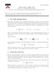
![Handout 3 [pdf] - University of Oxford Department of Physics](https://img.yumpu.com/46475432/1/190x245/handout-3-pdf-university-of-oxford-department-of-physics.jpg?quality=85)