Optimal control of the penicillin G fed-batch fermentation: An ...
Optimal control of the penicillin G fed-batch fermentation: An ...
Optimal control of the penicillin G fed-batch fermentation: An ...

You also want an ePaper? Increase the reach of your titles
YUMPU automatically turns print PDFs into web optimized ePapers that Google loves.
OPTIMAL CONTROL APPLICATIONS & METHODS, VOL. 15, 13-34 (1W)OPTIMAL CONTROL OF THE PENICILLIN G FED-BATCHFERMENTATION: AN ANALYSIS OF THE MODEL OFHEIJNEN ETAL.JAN F. VAN IMPEESA T - Department <strong>of</strong> Electrical Engineering, and Laboratory for Industrial Miembiology and Biochemistry,Katholieke Universiteit Leuven. Kardinaal Mercieraan 94, B-3WI Leuven, BelgiumBART M. NICOLAIDepartment <strong>of</strong> Agricultural Engineering, Katholieke Universiteit Leuven, Lcuve, BelgiumPETER A. VANROLLEGHEMDepartment <strong>of</strong> Agricultural Engineering. Universiteit Gent, Gent, BelgiumJAN A. SPRIETDepartment <strong>of</strong> Agricultural Engineering, Katholieke Universiteit Leuven. Leuven. BelgiumANDBART DE MOOR AND JOOS VANDEWALLEESA T - Department <strong>of</strong> Electrical Engineering, Katholieke Universiteit Lcuven. Leuven. BelgiumSUMMARYThis paper presents <strong>the</strong> application <strong>of</strong> optimal <strong>control</strong> <strong>the</strong>ory in determining <strong>the</strong> optimal feed rate pr<strong>of</strong>ilefor <strong>the</strong> <strong>penicillin</strong> G <strong>fed</strong>-<strong>batch</strong> <strong>fermentation</strong>, using a ma<strong>the</strong>matical model based on balancing methods.Since this model does not fulfil all requisites for standard optimal <strong>control</strong>, we propose a sequence <strong>of</strong> newmodels - that converges to <strong>the</strong> original one in a smooth way - to which <strong>the</strong> standard techniques areapplicable. The unusual optimization <strong>of</strong> some initial conditions is included. We <strong>the</strong>n state <strong>the</strong> conjecturethat allows us to obtain <strong>the</strong> optimal <strong>control</strong> for <strong>the</strong> original model. The enormous gains in productionand <strong>the</strong> vanishing <strong>of</strong> <strong>the</strong> characteristic biphasic behaviour through feed rate pr<strong>of</strong>ile optimization raisesome questions concerning <strong>the</strong> validity <strong>of</strong> this model. In this way this optimal <strong>control</strong> study can proveto be very useful for model discrimination purposes. Fur<strong>the</strong>rmore, ma<strong>the</strong>matical and microbial insightslead to <strong>the</strong> construction <strong>of</strong> a suboptimal heuristic strategy - which we show to be a limiting case <strong>of</strong> <strong>the</strong>optimal scheme - that can serve as a basis for <strong>the</strong> development <strong>of</strong> robust, model-independent, optimaladaptive <strong>control</strong> schemes.KEY WORDS <strong>Optimal</strong> <strong>control</strong> Non-linear systems Fed-<strong>batch</strong> <strong>fermentation</strong> processesBiotechnological modelling1. INTRODUCTIONThe design <strong>of</strong> high-performance model-based <strong>control</strong> algorithms for biotechnologicalprocesses is hampered by two major problems which call for adequate engineering solutions.First, <strong>the</strong> process kinetics are most <strong>of</strong>ten poorly understood non-linear functions, while <strong>the</strong>CCC 01 43-2087/94/ 01 001 3-220 1994 by John Wiley & Sons, Ltd.Received 20 December 1990Revised I1 January 1993
14 J. F. VAN IMPE ETAL.corresponding parameters are in general time-varying. Secondly, up till now <strong>the</strong>re is a lack <strong>of</strong>reliable sensors suited to real-time monitoring <strong>of</strong> process variables which are needed inadvanced <strong>control</strong> algorithms. Therefore <strong>the</strong> earliest attempts at <strong>control</strong> <strong>of</strong> a biotechnologicalprocess used no model at all. Successful state trajectories from previous runs which had beenstored in <strong>the</strong> process computer were tracked using open-loop <strong>control</strong>. Many industrial<strong>fermentation</strong>s are still operated using this method.During <strong>the</strong> last two decades, two trends for <strong>the</strong> design <strong>of</strong> monitoring and <strong>control</strong> algorithmsfor <strong>fermentation</strong> processes have emerged. ' In a jrst approach <strong>the</strong> difficulties in obtaining anaccurate ma<strong>the</strong>matical process model are ignored. In numerous papers classical methods (e.g.Kalman filtering, optimal <strong>control</strong> <strong>the</strong>ory, etc.) are applied under <strong>the</strong> assumption that <strong>the</strong> modelis perfectly known. Owing to this oversimplification, it is very unlikely that a real-lifeimplementation <strong>of</strong> such <strong>control</strong>lers - very <strong>of</strong>ten this implementation is already hampered bye.g. monitoring problems - would result in <strong>the</strong> predicted simulation results. In a secondapproach <strong>the</strong> aim is to design specific monitoring and <strong>control</strong> algorithms without <strong>the</strong> need fora complete knowledge <strong>of</strong> <strong>the</strong> process model, using concepts from e.g. adaptive <strong>control</strong> andnon-linear linearizing <strong>control</strong>. A comprehensive treatment <strong>of</strong> <strong>the</strong>se ideas can be found inReference 2 and <strong>the</strong> references cited <strong>the</strong>rein.We have shown how to combine <strong>the</strong> best <strong>of</strong> both trends into one unifying methodology foroptimization <strong>of</strong> biotechnological processes: optimal adaptive <strong>control</strong>. 3*4 This is motivated asfollows. Model-based optimal <strong>control</strong> studies provide a <strong>the</strong>oretical realizable optimum.However, <strong>the</strong> real-life implementation will fail in <strong>the</strong> first place owing to modellinguncertainties. On <strong>the</strong> o<strong>the</strong>r hand, model-independent adaptive <strong>control</strong>lers can be designed, but<strong>the</strong>re is a priori no guarantee for at least suboptimality <strong>of</strong> <strong>the</strong> results obtained. The gapbetween <strong>the</strong> two approaches is bridged in two steps. First, heuristic <strong>control</strong> strategies aredeveloped with nearly optimal performance under all conditions. These suboptimal <strong>control</strong>lersare based on biochemical knowledge concerning <strong>the</strong> process and on a careful ma<strong>the</strong>maticalanalysis <strong>of</strong> <strong>the</strong> optimal <strong>control</strong> solution. In a second step, implementation <strong>of</strong> <strong>the</strong>se pr<strong>of</strong>iles inan adaptive model-independent way combines excellent robustness properties with nearlyoptimal performance.As an example, we consider in this paper <strong>the</strong> development <strong>of</strong> a heuristic substrate feed rate<strong>control</strong>ler for <strong>the</strong> <strong>penicillin</strong> G <strong>fed</strong>-<strong>batch</strong> <strong>fermentation</strong> process, based on ma<strong>the</strong>matical andmicrobial insights. There are at least two unstructured models available in <strong>the</strong> literature thatallow for <strong>the</strong> optimization <strong>of</strong> <strong>the</strong> final <strong>penicillin</strong> amount with respect to <strong>the</strong> glucose feedingrate: <strong>the</strong> model <strong>of</strong> Heijnen et al. and <strong>the</strong> model <strong>of</strong> Bajpai and ReuD. The latter has beenanalysed in References 4 and 7. The analysis in this paper is based on <strong>the</strong> unstructuredma<strong>the</strong>matical model proposed by Heijnen et al. ' For <strong>the</strong> second step <strong>of</strong> <strong>the</strong> above approach,i.e. <strong>the</strong> adaptive implementation, we refer to References 3 and 4.Nowadays <strong>penicillin</strong> G is an almost common antibiotic; never<strong>the</strong>less <strong>the</strong> <strong>fermentation</strong>technology and <strong>the</strong> ma<strong>the</strong>matical description <strong>of</strong> <strong>the</strong> production process are still subjects <strong>of</strong>interest. The optimization <strong>of</strong> product formation during <strong>fed</strong>-<strong>batch</strong> <strong>fermentation</strong> as a part <strong>of</strong>total process <strong>control</strong> has gained renewed attention. *The category <strong>of</strong> secondary metabolites includes a large number <strong>of</strong> extremely valuablecompounds whose mass production has revolutionized public health in modern society. In thispaper <strong>the</strong> example <strong>of</strong> <strong>penicillin</strong> G <strong>fed</strong>-<strong>batch</strong> <strong>fermentation</strong> is only used as a vehicle forpresenting <strong>the</strong> basic ideas, methodology and results obtained. This <strong>fermentation</strong> process canbe considered representative for <strong>the</strong> whole class <strong>of</strong> processes with secondary metabolite^.^The paper is organized as follows. Section 2 presents <strong>the</strong> original model <strong>of</strong> Heijnen et al.and <strong>the</strong> modifications to make it suitable for standard optimal <strong>control</strong>, toge<strong>the</strong>r with <strong>the</strong>
PENICILLIN G FED-BATCH FERMENTATION 15statement <strong>of</strong> <strong>the</strong> complete optimization problem. We also formulate <strong>the</strong> basic conjecture <strong>of</strong>this paper. In Section 3 we develop for <strong>the</strong> first time <strong>the</strong> optimal feed rate pr<strong>of</strong>ile maximizing<strong>the</strong> final amount <strong>of</strong> product, in verifying <strong>the</strong> statement by Heijnen et al. that <strong>the</strong> glucose feedscheme is <strong>of</strong> crucial importance in obtaining high <strong>penicillin</strong> yields. Section 4 presents a physicalinterpretation <strong>of</strong> singular <strong>control</strong>, based on a ma<strong>the</strong>matical analysis <strong>of</strong> <strong>the</strong> optimal <strong>control</strong>solution. In Section 5 we derive a suboptimal strategy based on ma<strong>the</strong>matical and microbialknowledge, that is found to be a useful alternative for <strong>the</strong> optimal open-loop feed rate pr<strong>of</strong>ile.It opens perspectives for more reliable, adaptive, model-independent <strong>control</strong> schemes. Someconclusions are formulated in Section 6.Apart from <strong>the</strong> derivation <strong>of</strong> optimal <strong>control</strong> pr<strong>of</strong>iles for this model - which are importanton <strong>the</strong>ir own - we believe that <strong>the</strong> most important contributions <strong>of</strong> this paper are <strong>the</strong>following. The realizable gain due to feed pr<strong>of</strong>ile optimization is in <strong>the</strong> region <strong>of</strong> severalhundred per cent. Fur<strong>the</strong>rmore, <strong>the</strong> model is very sensitive towards different feeding policies.These results, toge<strong>the</strong>r with <strong>the</strong> fact that <strong>the</strong> commonly observed biphasic behaviour <strong>of</strong> <strong>the</strong><strong>penicillin</strong> <strong>fed</strong>-<strong>batch</strong> <strong>fermentation</strong> has disappeared after optimization, raise some questionsconcerning <strong>the</strong> validity <strong>of</strong> this model. In this way this optimal <strong>control</strong> study can prove to bevery useful for model discrimination purposes: optimization for model discrimination. Formore details see Reference 4. Secondly, <strong>the</strong> heuristic <strong>control</strong>lers introduced in Section 5 havean excellent performance in all cases. Moreover, since <strong>the</strong> <strong>control</strong> objective (namely to keep<strong>the</strong> specific growth rate constant during <strong>the</strong> production phase) is obtained independently <strong>of</strong> <strong>the</strong>exact analytical expressions for <strong>the</strong> specific rates, <strong>the</strong>se <strong>control</strong>lers can serve indeed as a basisfor <strong>the</strong> development <strong>of</strong> model-independent <strong>control</strong> algorithms. This is elaborated in detail inReferences 3 and 4: optimal adaptive <strong>control</strong>.2.1. The original model equations2. THE MODEL OF HEIJNEN ETAL.Heijnen et al. used <strong>the</strong> following steps in <strong>the</strong> construction <strong>of</strong> a simple unstructured modelfor <strong>the</strong> <strong>penicillin</strong> G <strong>fed</strong>-<strong>batch</strong> <strong>fermentation</strong> process: (i) definition <strong>of</strong> relevant compounds in <strong>the</strong><strong>penicillin</strong> <strong>fermentation</strong>, (ii) specification <strong>of</strong> chemical composition and specific enthalpies, (iii)formulation <strong>of</strong> elemental balances and <strong>the</strong> enthalpy balance (one <strong>of</strong> <strong>the</strong> most interestingfeatures <strong>of</strong> this approach), (iv) formulation <strong>of</strong> mass balances for individual compounds, (v)formulation <strong>of</strong> <strong>the</strong> weight balance and (vi) selection <strong>of</strong> <strong>the</strong> kinetic equations (in this case basedon a literature survey). Their research resulted in <strong>the</strong> following continuous-time model which<strong>the</strong>y believe to be <strong>of</strong> great possible help in <strong>the</strong> optimization <strong>of</strong> <strong>the</strong> process:dSdX-= -ux+u, - = px, -= dPdt dt dt?rx-khPwithSXPG-=- dGdtCs,inu - 0-OOO8G - O-044rc + 0*068rn + 0*392rs, + 0-032r0 + 0.687rXamount <strong>of</strong> substrate (glucose) in broth (mol)amount <strong>of</strong> cell mass in broth (mol dry weight)amount <strong>of</strong> product (<strong>penicillin</strong>) in broth (mol)total broth weight (kg)(1)
16 J. F. VAN lMPE ETAL.substrate feed rate (mol h-')glucose concentration in feed stream (mol kg-')specific substrate consumption rate (mol (mol dry weight)-' h- ')specific growth rate (h-')specific production rate (mol (mol dry weight)-' h-')<strong>penicillin</strong> hydrolysis constant (h- ' )net rate <strong>of</strong> C02 conversion (mol h-')net rate <strong>of</strong> nitrogen source conversion (mol h-')net rate <strong>of</strong> oxygen conversion (mol h-')net rate <strong>of</strong> sulphate source conversion (mol h-').Observe that this model is written in a (mol, kg) unit system: concentrations <strong>of</strong> substrate,biomass and product (denoted Cs, Cx and C, respectively) are expressed with respect to totalbroth weight G. In <strong>the</strong> last equation, terms with a positive sign are due to <strong>the</strong> input <strong>of</strong> glucose,nitrogen source, sulphate source, oxygen and precursor respectively. Terms with a negativesign represent evaporation and carbon dioxide production respectively. For more details seeReference 5. The specific rates u, p and u are modelled as follows.1.The specific substrate consumption rate u is modelled using a Monod-type relationship92.3.withQs,maxKsmaximum specific sugar uptake rate (mol (mol dry weight)-' h-')Monod constant for sugar uptake (mol kg-').The specific production rate u is assumed to be directly coupled with <strong>the</strong> specific growthrate p, following a Blackman-type relation'withQp,m=bfitmaximum specific production rate (mol (mol dry weight)-' h-')critical specific growth rate (h-').The (overall) specific growth rate p is given bywithmYdsYPlsp = Y du - m - u/ Yp~s)overall specific maintenance demand (mol (mol dry weight)- ' h-')biomass-on-substrate yield coefficient (mol dry weight mol- ' )product-on-substrate yield coefficient (mol mol- ' )which represents an endogenous metabolism viewpoint. This means that <strong>the</strong> energysupply for maintenance <strong>of</strong> living biomass and for product syn<strong>the</strong>sis is assumed to be dueto combustion <strong>of</strong> part <strong>of</strong> <strong>the</strong> biomass.Table I shows <strong>the</strong> parameters and initial conditions used in all simulations; a is <strong>the</strong> totalamount <strong>of</strong> substrate available for <strong>fermentation</strong>. The expressions for <strong>the</strong> rates r,, rn, r,, and r,,can be found in Reference 5.(3)(4)
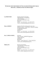
18 J. F. VAN IMPE ETAL.~=o(lO-~). Using <strong>the</strong> exact expressions for <strong>the</strong> specific rates r,, r,, r, and r,, (seeReference5) on <strong>the</strong> right-hand side <strong>of</strong> equation(l), it can be verified that under <strong>the</strong>seconditions <strong>the</strong> second most important contribution comes from <strong>the</strong> term representingevaporation. Thus <strong>the</strong> above dynamic equation for C, can be written asdt+ O*OOOSC, + lower-order termsWith u <strong>of</strong> <strong>the</strong> order <strong>of</strong> magnitude <strong>of</strong> 1OOO mol h-', <strong>the</strong> term 0-OOOSC, has negligible influenceon <strong>the</strong> dynamics <strong>of</strong> C, and thus on <strong>the</strong> dynamics <strong>of</strong> all specific rates.Thus, in optimizing <strong>the</strong> final product amount P(tf) with respect to <strong>the</strong> glucose feedingpolicy, we will omit all <strong>the</strong>se terms to simplify <strong>the</strong> analytical developments. The original model<strong>the</strong>n reduces todS-= -aX+u,dt_--dXdPdG 1- = pX, -==X-khP,dt dt dt G,in<strong>An</strong>o<strong>the</strong>r advantage <strong>of</strong> this model structure is that we can take care <strong>of</strong> an isoperimetricconstraint on <strong>the</strong> input without introducing an additional state equation.As an example, using SO = 5500 mol and a constant input u = 1OOO mol h-' for 200 h, weobtain P(tf) = 3001 - 12 mol on using <strong>the</strong> complete equation for G in (l), but a value which isonly 0.03% smaller on using only <strong>the</strong> first term as in (5). The simulation results using <strong>the</strong>simplified model are shown in Figure 2. Some comments are in order here.1. Up to now <strong>the</strong> <strong>penicillin</strong> <strong>fermentation</strong> - when operated in <strong>fed</strong>-<strong>batch</strong> mode - is most<strong>of</strong>ten classified in <strong>the</strong> group <strong>of</strong> product formation processes <strong>of</strong> <strong>the</strong> non-growth-associatedtype. In agreement with <strong>the</strong> experimentally observed behaviour, <strong>the</strong> process is assumedto consist <strong>of</strong> two phases: a phase <strong>of</strong> rapid growth with almost no product formation(trophophase) and a phase with limited growth in which <strong>the</strong> product is formed(idiophase). The simulation results for C,(t), Cx(t) and P(t) are obviously in agreementwith this biphasic description. However, Heijnen et al. obtained <strong>the</strong>se results on <strong>the</strong>assumption <strong>of</strong> a direct coupling between specific growth rate and specific rate <strong>of</strong> productformation (see equation (3)). The p- and ?r-pr<strong>of</strong>iles in Figure 2 illustrate some <strong>of</strong> <strong>the</strong>seideas. Heijnen et al. <strong>the</strong>refore concluded that <strong>the</strong> apparent separation between(5)0 20 40 60 80 100 170 140 160 180 200'lime [h]Figure 2. Constant glucose feed rate and corresponding cell, glucose, product, p- and *-pr<strong>of</strong>iles. Scaling: C, x 10,c, x 2, p/103, c/105, x 40, x 10'
PENICILLIN G FED-BATCH FERMENTATION 19production and growth phases does not necessarily mean that <strong>penicillin</strong> production is <strong>of</strong><strong>the</strong> non-gro wth-associated type.2. <strong>An</strong>o<strong>the</strong>r feature <strong>of</strong> <strong>the</strong> simulation results is an apparent lag phase in <strong>the</strong> <strong>penicillin</strong>production curve <strong>of</strong> about 20 h. Observe that this was not introduced a priori in <strong>the</strong>model. Heijnen et al. concluded that it remains possible that <strong>the</strong>re is in reality no reallag in <strong>the</strong> beginning <strong>of</strong> <strong>penicillin</strong> production.3. <strong>An</strong>o<strong>the</strong>r modelling approach that has been followed is <strong>the</strong> assumption <strong>of</strong> a relationshipbetween mycelial age and its productivity. Most <strong>of</strong>ten <strong>the</strong> product activity is assumed todecrease at high mycelial age. '' In this way <strong>the</strong> decreasing ?r-curve (Figure 2) during <strong>the</strong>production phase can be modelled. However, Heijnen et al. did not model such an agedependence. In <strong>the</strong>ir viewpoint <strong>the</strong> decreasing ?r-pr<strong>of</strong>ile may very well be explained ei<strong>the</strong>rby dilution due to increasing broth weight or by hydrolysis <strong>of</strong> <strong>penicillin</strong> to penicilloicacid.Heijnen et al. concluded that with <strong>the</strong>ir growth-coupled <strong>penicillin</strong> production most <strong>of</strong> <strong>the</strong>phenomena observed in practice - which have <strong>of</strong>ten led to <strong>the</strong> assumption <strong>of</strong> non-growthassociatedor age-dependent <strong>penicillin</strong> productivity - can be adequately described. We wilIcome back to <strong>the</strong>se interpretations in subsequent sections. However, from <strong>the</strong> ma<strong>the</strong>maticalpoint <strong>of</strong> view <strong>the</strong> commonly observed separation between growth and production phases isquite a useful feature in optimizing <strong>the</strong> process.2.3. Statement <strong>of</strong> <strong>the</strong> optimization problemHeijnen et al. used <strong>the</strong>ir model to illustrate that <strong>the</strong> feed rate projile during <strong>fermentation</strong>is <strong>of</strong> vital importance in <strong>the</strong> realization <strong>of</strong> a high production rate throughout <strong>the</strong> duration <strong>of</strong><strong>the</strong> <strong>fermentation</strong>. This statement was based on <strong>the</strong> following set <strong>of</strong> <strong>control</strong>s for 200 h: (i) aconstant input u(t) = loo0 mol h-' (<strong>the</strong> results <strong>of</strong> which are shown in Figure 2), (ii) a linearlyincreasing input u(t) = 500 + 5t mol h- ' and (iii) a linearly decreasing inputu(t) = 1500 - 5t mol h-'. The initial substrate amount was fixed at SO = 5500 mol. Using <strong>the</strong>simplified model, we obtain P(tf) = 3001, 5883 and 89 mol respectively. Although Heijnenet al. did not consider o<strong>the</strong>r feeding strategies in an attempt to obtain <strong>the</strong> optimal substratefeeding pr<strong>of</strong>ile, <strong>the</strong> above results indicate that <strong>the</strong> present model allows indeed for <strong>the</strong>optimization <strong>of</strong> <strong>the</strong> final amount <strong>of</strong> product, P(tf), with respect to <strong>the</strong> glucose feed ratescheme.We now formulate <strong>the</strong> problem <strong>of</strong> optimizing <strong>the</strong> final product amount as an optimal<strong>control</strong> problem. With <strong>the</strong> definitions (superscript T denotes <strong>the</strong> transpose <strong>of</strong> a vector)x = (XI xz ~3 ~4)'s (S X P G)'khP 0)'b= (bl bt b3 b4)' 4 (1 0 0 l/CS,in)'f = (fi fz f3 f4)T 4 (-OX h x ?rx-we obtain <strong>the</strong> following state space model linear in <strong>the</strong> <strong>control</strong> u:-= dxdtf(x)+ buNumerical values for <strong>the</strong> initial conditions are given in Table I. xz(0) and x3(0) are given; <strong>the</strong>initial amount <strong>of</strong> substrate, x1(0), is free. xi(0) and xq(0) are related byX4(0) = G* + Xi (O)/Cs,in (7)where G* denotes <strong>the</strong> given initial weight without substrate (G* = 98020 kg (Table I)).
PaPa20 J. F. VAN IMPE ETAL.The optimization problem is to determine for <strong>the</strong> given set <strong>of</strong> differential equations (6) <strong>the</strong>optimal initial state xo* and <strong>the</strong> optimal feed rate pr<strong>of</strong>ile u*(t) that minimize <strong>the</strong> performanceindexJ[u,xol =g[X(tf)l 2 -x3(tf) (8)i.e. maximize <strong>the</strong> final amount <strong>of</strong> product, subject to <strong>the</strong> following constraints.(i) to = 0, tf is free.(ii) All variables have to be kept positive:W E[O,tf]: Xi(t) 20 for i= 1, ..., 4 A u(t) 20(iii) The total amount <strong>of</strong> substrate available, a, is fixed, i.e.x1(0) + 1" u(t) dt = atoThe last isoperimetric constraint on <strong>the</strong> input is equivalent to a physical constraint <strong>of</strong> <strong>the</strong> form(see <strong>the</strong> simplified differential equation for total broth weight G in (5))2.4. The basic conjecturex4(tf) = G(tf) = Gf, Gf fixed (10)As can be easily seen from mode1,equation (3) and Figure 1, <strong>the</strong> specific production rate aexhibits a corner at p = pcrit or equivalently at C, = Cs,crit. As a result, some partial derivativesa fi/axj are not continuous. Thus we cannot apply standard optimal <strong>control</strong> <strong>the</strong>ory. Tocircumvent this problem, we replace <strong>the</strong> piecewise smooth Blackman-type kinetics rb) in (3)by a family <strong>of</strong> completely smooth curves that converges as a function <strong>of</strong> one parameter to <strong>the</strong>original kinetics. This is basically inspired by <strong>the</strong> following conjecture.(9)Conjecture ISuppose we have a convergent sequence <strong>of</strong> models (A(p)), where p is a set <strong>of</strong> parameterslim ~ ( p e ) 4P +Suppose that for every model A (p) with p # PO we can determine <strong>the</strong> optimal <strong>control</strong> u(p, t)that minimizes some cost index J[ul with standard optimal <strong>control</strong> <strong>the</strong>ory. Then <strong>the</strong> sequence<strong>of</strong> optimal <strong>control</strong>s (u(p, t)) is convergent:P +lim u(p,t) 2 uo(t)Moreover, this limit uo(t) is <strong>the</strong> optimal <strong>control</strong> for model Jtlo minimizing J[u].It can be easily illustrated that proving Conjecture 1 in general is not possible. InReference 4 we give an outline <strong>of</strong> <strong>the</strong> pro<strong>of</strong> if some additional assumptions are satisfied.However, it may be very difficult in practice to verify all <strong>the</strong>se assumptions.Because at this time more general results are still lacking, we can proceed as follows for aparticular optimal <strong>control</strong> problem characterized by a model 4. We assume a priori thatConjecture 1 holds. Then we select a model &(pa) suficiently close to <strong>the</strong> limit model &,i.e. we choose n sufficiently large. If we are able to determine <strong>the</strong> optimal <strong>control</strong> solution
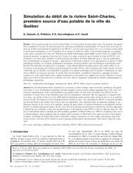
PENICILLIN G FED-BATCH FERMENTATION 21using model ufl(pn), <strong>the</strong>n this solution will be at least an excellent approximation for <strong>the</strong>optimal <strong>control</strong> to <strong>the</strong> limit model &. In <strong>the</strong> following it will be illustrated that <strong>the</strong> validity<strong>of</strong> Conjecture 1 can always be verified a posteriori.2.5. A modified modelConsider <strong>the</strong> following relationship between p and T, a Dabes-type kinetics,’ withparameters A and B:or, in ano<strong>the</strong>r way,p=A’R+BTQp.max - TAT’ - (Qp,maxA + B + p)* + Qp,maxfi = 0Solving this quadratic equation for a and taking <strong>the</strong> root with negative sign - we want T = 0at p = 0 as in <strong>the</strong> original kinetics (3) - leads to.or) =Qp,maxA + B + p - J[(Qp.maxA2AWe now eliminate one parameter, say A, by solving+ B + p)2 - 4AQp.maxpIwhich imposes that <strong>the</strong> derivative <strong>of</strong> T at p = 0 must be equal to <strong>the</strong> value derived fromequation (3). The solution isand thus we obtainaOt) = Qp,maxpcrit - BA=-------QpmaxP + firit - J[b + pcrit)2 - 4tpcrit - B)PI2(pcrit - B)which is <strong>the</strong> desired family <strong>of</strong> smooth curves, where B, which must lie in <strong>the</strong> range0 < B c krit, is <strong>the</strong> only parameter.Let us consider now <strong>the</strong> boundaries for <strong>the</strong> parameter B. For B -+ bcrit, A tends to zero and<strong>the</strong> above equation becomes undetermined. However, solving <strong>the</strong> original relation (1 1) for awith A = 0 delivers <strong>the</strong> Monod-type law(12)which is <strong>of</strong> course also a completely smooth relationship. On <strong>the</strong> o<strong>the</strong>r hand, as B + 0,equation (12) reduces towhich is in fact ano<strong>the</strong>r form <strong>of</strong> <strong>the</strong> original model (3). Thus we can refine <strong>the</strong> boundaries forB to 0 < B Q brit.We conclude that we have constructed a one dimensional family <strong>of</strong> curves - and thus a
22 J. F. VAN IMPE ETAL.XIO-43.53.0 0.002 0.004 0.006 0.008 0.01 0.012 0.014 0.016 0.018 0.02PIlhlFigure 3. Dabes-type kinetics rh) for various values <strong>of</strong> parameter Bfamily <strong>of</strong> models - that is completely smooth within <strong>the</strong> given boundaries <strong>of</strong> <strong>the</strong> parameterB, thus assuring <strong>the</strong> continuity <strong>of</strong> afi/ax, for all i and j. Moreover, as BZO, we comearbitrarily close to <strong>the</strong> original model. In Figure 3 we show some members <strong>of</strong> <strong>the</strong> family (12)for different values <strong>of</strong> B. From <strong>the</strong> numerical point <strong>of</strong> view, setting B = lo-" in equation (12)is a very accurate approximation in simulating <strong>the</strong> original Blackman-type kinetics (3).Obviously, we can now determine <strong>the</strong> optimal <strong>control</strong> u*(B, t) for every B within <strong>the</strong> givenboundaries ]O,pcrit] using standard optimal <strong>control</strong> <strong>the</strong>ory. For <strong>the</strong> original model -corresponding to B = 0 - we will make use <strong>of</strong> Conjecture 1.Observe that from a ma<strong>the</strong>matical point <strong>of</strong> view <strong>the</strong> approximation <strong>of</strong> <strong>the</strong> piecewise smoothBlackman-type kinetics (3) can be done by any family <strong>of</strong> completely smooth curves thatconverges to <strong>the</strong> original kinetics. Clearly, <strong>the</strong> optimal <strong>control</strong> solution for <strong>the</strong> original kineticsis independent <strong>of</strong> this choice. However, from a biochemical point <strong>of</strong> view a sharp corner in7 at p = pcrit must be considered as a first approximation <strong>of</strong> real-life <strong>fermentation</strong> conditions.By using Dabes-type kinetics, each model <strong>of</strong> <strong>the</strong> sequence (.<strong>An</strong>) can be assigned a meaningfulinterpretation.3. OPTIMAL CONTROL USING THE MODIFIED MODEL3.1. Solution <strong>of</strong> <strong>the</strong> two-point boundary value problemThe given optimization problem can be formulated within <strong>the</strong> frame <strong>of</strong> <strong>the</strong> minimumprinciple l2*I3 as a two-point boundary value problem (TPBVP). The Hamiltonian Xfor thisproblem isThe adjoint vector X satisfies <strong>the</strong> following system <strong>of</strong> differential equations:
PENICILLIN G FED-BATCH FERMENTATION 23can be obtained by substituting equation (12) in equation (4) and calculating <strong>the</strong> implicitpartial derivatives with respect to XI and x4 respectively.The state equations (6) toge<strong>the</strong>r with <strong>the</strong> costate equations (15) constitute a set <strong>of</strong> 2 x 4 firstorderdifferential equations. The required boundary conditions are as follows.(i) x~(0) and x3(0) are given.(ii) XI (0) and xq(0) are interrelated by equation (7).(iii) Since xl(0) and n(0) are not given explicitly, it can be shown that <strong>the</strong> followingcondition must be ~atisfied:~(iv) xq(tf) is given by equation (10).(v) X;(tf), i = 1, ..., 3, are given byXI@) + h(O)/Cs,in $(O) = 0or, using (8),(Xl(tf) XZ(tf) Xdtr))'=(O 0 -1)' (16)As stated in <strong>the</strong> minimum principle, an extremal <strong>control</strong> follows from <strong>the</strong> minimization <strong>of</strong> <strong>the</strong>Hamiltonian .34? in (14) over all admissible <strong>control</strong> functions while satisfying <strong>the</strong> given TPBVP:min N(X*, A*, u) = s(x*, A*, u*)all admissible uNote that since all conditions are necessary conditions, we can only obtain extremol solutions(x*, X*, u*) which must be checked for optimality. Because <strong>the</strong> state equations (6) and <strong>the</strong> costindex (8) are time-invariant , <strong>the</strong> Hamiltonian .X' remains constant along an extremaltrajectory. Since <strong>the</strong> final time tf is free, we know that a'= 0.As already mentioned, <strong>the</strong> original kinetics (2)-(4) represent a degenerate case <strong>of</strong> a<strong>fermentation</strong> process with monotonic specific growth rate p and non-monotonic specificproduction rate ?r - <strong>the</strong> corner point is a degenerate maximum - for which an efficientcomputational algorithm yielding <strong>the</strong> optimal <strong>control</strong> has been derived in Reference 4.However, <strong>the</strong> original model is only piecewise smooth, so this algorithm cannot be useddirectly because it requires <strong>the</strong> computation <strong>of</strong> <strong>the</strong> partial derivatives (up to second order) <strong>of</strong><strong>the</strong> right-hand side <strong>of</strong> model equations (6) with respect to <strong>the</strong> state.We verify now that <strong>the</strong> computational algorithm can be used for any model with a specificproduction rate kinetics within <strong>the</strong> family <strong>of</strong> completely smooth curves (12). The optimalsolution using <strong>the</strong> original model is <strong>the</strong>n obtained by considering <strong>the</strong> limitas stated in Conjecture 1.Iim u*@, t) 4 U*(B = 0, t)B>,OBecause <strong>the</strong> Hamiltonian .34? is linear in <strong>the</strong> <strong>control</strong> input u, <strong>the</strong> minimum principle fails toprovide <strong>the</strong> solution on any singular interval [ti, ti+l] where <strong>the</strong> function I,L remains zero. Ithas been shown4 that this problem is a singular problem <strong>of</strong> order two. In that case <strong>the</strong> singular<strong>control</strong> can be calculated by solving
24 J. F. VAN IMPE ETAL.for <strong>the</strong> <strong>control</strong> input u. We obtainwithdkaf--baxIt can be verified that for all kinetics (12) <strong>the</strong> denominator <strong>of</strong> <strong>the</strong> singular <strong>control</strong> uri,(t) isdifferent from zero. Since both <strong>the</strong> numerator and <strong>the</strong> denominator are linear in <strong>the</strong> costatevariables X and <strong>the</strong>re exist three linear homogeneous equations between <strong>the</strong>m, we know that<strong>the</strong> optimal <strong>control</strong> along a singular arc is a non-linear feedback law <strong>of</strong> <strong>the</strong> state variables xonly. These three equations are3 zz Xfd = 0,dt$t = X'b = 0, 6 = X'f = 0For this problem it can be seen that XS has disappeared from Usiw(t), since fs = 0. Thus <strong>the</strong>first equation can be omitted and <strong>the</strong> last two can be solved as(" 01 f2) 02 (XI) Xzafiafi= - (;)A3pi bl - + b4 -, i = 1, ..., 3ax,ax4Consider <strong>the</strong> case <strong>of</strong> an unbounded input u and an unconstrained state vector x. As shown inReference 4, <strong>the</strong> problem <strong>the</strong>n reduces to <strong>the</strong> two-dimensional optimization <strong>of</strong> <strong>the</strong> initialamount <strong>of</strong> substrate SO and <strong>the</strong> time instant t2 at which <strong>the</strong> switch from <strong>batch</strong> to singular<strong>control</strong> occurs, <strong>the</strong> optimal <strong>control</strong> sequence being <strong>batch</strong>-singular arc-<strong>batch</strong>. The followingstraightforward computational algorithm has been pr~posed.~*'~AlgorithmStep I . Make a guess <strong>of</strong> SO or, equivalently, determine <strong>the</strong> amount <strong>of</strong> substrate, CYgmwth,consumed during <strong>the</strong> growth phase.Step 2. Make a guess <strong>of</strong> 22. Integrate <strong>the</strong> state equations (6) from t = 0 to t = t2 with u(t) = 0.This completes <strong>the</strong> growth phase.Step 3. Integrate <strong>the</strong> state equations (6) using <strong>the</strong> above-determined singular <strong>control</strong> (17)until all substrate available, a in (9), is added or, equivalently, until <strong>the</strong> bioreactor iscompletely filled (equation (10)) at time t = 23.Step 4. Complete <strong>the</strong> integration with u(t) = 0 until <strong>the</strong> stopping condition - depending on<strong>the</strong> cost index - is satisfied at time t = Cf. This completes <strong>the</strong> production phase. Store <strong>the</strong> value<strong>of</strong> <strong>the</strong> cost index J[u,xo] in (8).Step 5. Repeat Steps 2-4 considering t2,new = t2,old 2 62, with 6t as small as required. Save<strong>the</strong> time f2 at which <strong>the</strong> cost index J[u,xo] in (8) reaches its minimum.
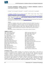
PENICILLIN G FED-BATCH FERMENTATION 25Step 6. Repeat Steps 1-5 with a new guess <strong>of</strong> SO in order to minimize J[u, XO].For <strong>the</strong> performance measure under consideration, equation (8), it can be easily shown (byusing (14) and (16)) that <strong>the</strong> stopping condition for this case is dP/dt(tr)=O, as could beexpected. In <strong>the</strong> case <strong>of</strong> a constraint on <strong>the</strong> <strong>control</strong> u and/or <strong>the</strong> state vector x, only someminor modifications are required, <strong>the</strong> algorithm itself remaining a two-dimensional search. Adetailed analysis <strong>of</strong> this algorithm in comparison with <strong>the</strong> algorithm proposed by Lim et al. l5toge<strong>the</strong>r with a verification <strong>of</strong> all necessary conditions for optimality can be found inReference 4. The main difference from <strong>the</strong> algorithm <strong>of</strong> Lim et al. is that we do not make use<strong>of</strong> <strong>the</strong> costate variables, whatever <strong>the</strong> performance index under consideration.3.2. Simulation resultsWe now present some results obtained with <strong>the</strong> above computational algorithm. Weconcentrate on two specific values <strong>of</strong> <strong>the</strong> parameter B (i) B = lo-" as an approximation <strong>of</strong><strong>the</strong> original Blackman-type kinetics (3) and (ii) <strong>the</strong> o<strong>the</strong>r extremal value B = krit = lo-', where~ ( p reduces ) to <strong>the</strong> Monod-type law (13).3.2.1. B = 10-". In <strong>the</strong> left plot <strong>of</strong> Figure 4 we have visualized <strong>the</strong> actions taken by <strong>the</strong>For every SO <strong>the</strong> optimal switch time t2 has beencomputational algorithm for B= lo-''.calculated. As a consequence, we obtain <strong>the</strong> corresponding values for P(tr) and tr. Clearly, <strong>the</strong>optimal couple (&*, t;) is <strong>the</strong> one which maximizes P(tr). Observe <strong>the</strong> quadratic behaviour <strong>of</strong>P(tr) as a function <strong>of</strong> SO, so that <strong>the</strong>re exists a unique optimal solution to this problem.Observe that <strong>the</strong>re exists a lower limit Smin on <strong>the</strong> possible values for SO, corresponding totz = 0. In that case <strong>the</strong> complete initial state xo is on <strong>the</strong> singular hyperplane, so singular<strong>control</strong> starts immediately. Note that SO = a corresponds to a complete <strong>batch</strong> <strong>fermentation</strong>:tr = t3 = tz, with u(t) = 0 for ali t. Even for values <strong>of</strong> SO in <strong>the</strong> neighbourhood <strong>of</strong> a, <strong>the</strong>condition dP/dt = 0 is never met before t = t2. As a result, we can indeed apply <strong>the</strong> proposedcomputational algorithm to <strong>the</strong> whole possible range SO E [Smin, a]. A derived benefit is <strong>of</strong>course that a good starting value for SO is not required for <strong>the</strong> algorithm to converge. Somenumerical values for <strong>the</strong> optimal <strong>control</strong> are summarized in Table 11. The right plot <strong>of</strong> Figure 4100 0.2 0.4 0.6 0.8 1 1.2 1.4 1.6 1.8 2s(w Id1.LO+Figure 4. B= lo-". Left plot: extremal values for P(tf), t2 and tf as functions <strong>of</strong> SO. Scaling: tJSO, rf/500,(P(tr) - 8150)/180. Right plot. optimal glucose feed rate and corresponding cell, glucose, product, T- and p-pr<strong>of</strong>iles.Scaling: c, x 300, c, x 5, q103, p x 100, r x 2 x lo4, u/300Time [h]
26 J. F. VAN IMPE ET AL.Table 11. <strong>Optimal</strong> and suboptimal <strong>control</strong> resultsB =<strong>Optimal</strong> <strong>control</strong> <strong>Optimal</strong> 3000 22.321 349-987 350.101 8319.461 1-oooOHeuristic <strong>control</strong> pcrit 3000 22.337 350.037 350.151 8319.239 0.9999B= lo-*<strong>Optimal</strong> <strong>control</strong> <strong>Optimal</strong> 326 0 277.205 277.320 4564.455 1.ooOOHeuristic <strong>control</strong> <strong>Optimal</strong> 1000 12.225 304.665 304.792 4553.437 0 * 9976Heuristic <strong>control</strong> kLcdt 7000 29.573 292-890 292.995 4399.589 0.9639shows <strong>the</strong> corresponding time pr<strong>of</strong>iles. Let us make <strong>the</strong> following remarks.1. From Table11 we note that <strong>the</strong> optimal initial substrate amount SO is ra<strong>the</strong>r low ascompared with <strong>the</strong> total amount available, (Y = 205 500 mol, resulting in a small first<strong>batch</strong> phase [0, t ~] <strong>of</strong> 22-32 h. In fact, <strong>the</strong> singular interval [t2, t3] takes most <strong>of</strong> total<strong>fermentation</strong> time tf. The terminating <strong>batch</strong> phase [t3, t f ] is negligibly small.2. From <strong>the</strong> pr<strong>of</strong>iles for Cx(t) and P(t) (Figure 4) we conclude that although <strong>the</strong> optimal<strong>control</strong> algorithm is based on <strong>the</strong> conjecture <strong>of</strong> a biphasic process, this biphasicbehaviour has disappeared almost completely as compared with e.g. <strong>the</strong> results for <strong>the</strong>constant strategy <strong>of</strong> Figure 2. Principally this is due to <strong>the</strong> structure <strong>of</strong> <strong>the</strong> specificproduction rate 7r in (3), which represents a direct coupling between product syn<strong>the</strong>sis andbiomass growth.3. On <strong>the</strong> singular arc [t2, t3] <strong>the</strong> optimal <strong>control</strong> seems to maintain p at <strong>the</strong> lowest possiblevalue (p = brit) which still guarantees <strong>the</strong> maximum possible value for 7r. We have shownin Reference 4 that during singular <strong>control</strong> C,(t) (and thus p(t) and a(t)) is time-varying,since kh # 0. However, kh is so small that <strong>the</strong> resulting variations in C, (and thus in pand a) are in fact negligible, so that <strong>the</strong>y cannot be detected on this plot.4. It is important to see that <strong>the</strong> optimal <strong>control</strong> keeps ?r on its maximum value for all t < l3.This will be at <strong>the</strong> basis <strong>of</strong> suboptimal pr<strong>of</strong>iles presented in Section 5.5. In order to evaluate <strong>the</strong> performance <strong>of</strong> <strong>the</strong> optimal <strong>control</strong> u*(t), we need somereference. Since we do not penalize <strong>the</strong> total <strong>fermentation</strong> time tf in <strong>the</strong> cost index J[u, xo]in (8), a good choice might be <strong>the</strong> outcome <strong>of</strong> a constant <strong>control</strong> with tf = t; r:denoting<strong>the</strong> optimal <strong>fermentation</strong> time. For convenience we take So,,f = 0 mol. Then we define<strong>the</strong> gain F3 (Yo) asFor B= lo-'' a constant <strong>control</strong> for 350.101 h with SO= 0 produces 1981.283 mol<strong>penicillin</strong>. Thus for <strong>the</strong> optimal <strong>control</strong> u*(t) E u*(B= 0, t) we obtain a gain% = 319-9070. Consider now a constant feed rate strategy. Optimizing <strong>the</strong> initial substrateamount SO and <strong>the</strong> final time tf leads to SO= 90.156 mol, tf= 129.688 h andPf= 3779.012 mol. Observe that this optimal final amount is still far away from <strong>the</strong>optimal <strong>control</strong> result. From this simple parametric optimization we can conclude thatthis model is very sensitive to wards diflerent feeding policies.Observe <strong>the</strong> enormous increase in <strong>the</strong> final product amount P(tf), which may suggest some
PENIClLLlN G FED-BATCH FERMENTATION 27questions concerning <strong>the</strong> validity <strong>of</strong> <strong>the</strong> model <strong>of</strong> Heijnen et al. under conditions imposed byapplying <strong>the</strong> optimal feed rate. Since up to now <strong>the</strong> <strong>penicillin</strong> <strong>fermentation</strong> has been recognizedthrough all experiments as an intrinsically biphasic process, it seems unlikely that <strong>the</strong> obtained<strong>control</strong> put into practice would result in a quasi-monophasic <strong>fermentation</strong> while producingsuch a high gain. We conclude that <strong>the</strong> results obtained using optimal <strong>control</strong> <strong>the</strong>ory suggestsome possible shortcomings in this model: optimization for model discrimination. A deeperstudy <strong>of</strong> this model in comparison with <strong>the</strong> model <strong>of</strong> Bajpai and Red6 can be found inReference 4.3.2.2. B=brif= ZO-'. We now give <strong>the</strong> analogous results for <strong>the</strong> o<strong>the</strong>r extremal valueB = perit = lo-' in order to demonstrate that <strong>the</strong> computational algorithm can be applied toevery model with 0 < B < hrit. The left plot <strong>of</strong> Figure 5 shows <strong>the</strong> evolution <strong>of</strong> tz and thusP(tr) and tf as functions <strong>of</strong> SO. Observe that <strong>the</strong> optimal couple (S:, t?) corresponds to tz = 0;in o<strong>the</strong>r words, <strong>the</strong> optimal initial state lies on <strong>the</strong> singular hyperplane itself. As a consequence,<strong>the</strong> separation between growth and production phases has disappeared completely. This is alsoillustrated by <strong>the</strong> time pr<strong>of</strong>iles <strong>of</strong> <strong>the</strong> right plot <strong>of</strong> Figure 5. In this case both u and ?r are <strong>of</strong>Monod type: <strong>the</strong> corner point in ?r has disappeared completely (see Figure 3). However, <strong>the</strong>optimal solution does not consist <strong>of</strong> adding all substrate available at t = 0 followed by a <strong>batch</strong>phase as could be expected at first sight. The main reason is <strong>the</strong> following. Combiningequations (2) and (4) with (13). we can verify that <strong>the</strong> resulting expression for u as a function<strong>of</strong> C, does not satisfy an equation <strong>of</strong> <strong>the</strong> formu(Cs) = Yp/xp(C,)In o<strong>the</strong>r words, this is not a case <strong>of</strong> completely growth-associated production.For this value <strong>of</strong> B <strong>the</strong> lower limit &in is equal to <strong>the</strong> optimal value $. Note again that <strong>the</strong>condition dP/dt = 0 is never met before t = tt, so we can indeed apply <strong>the</strong> proposed algorithmto <strong>the</strong> whole interval So€ [Smin,a]. Some numerical values for <strong>the</strong> optimal <strong>control</strong> aresummarized in Table 11.Observe that on <strong>the</strong> singular arc <strong>the</strong> variations in u and p (and thus in C,) with respect totime are more pronounced than in <strong>the</strong> case <strong>of</strong> B = lo-", although kh has not been changed.We conclude that <strong>the</strong> model structure itself also plays an important role in <strong>the</strong> amplitude <strong>of</strong><strong>the</strong>se variations.1, , 10,0 0.5 1 1.5 1 1.5 3 3.5YW Imdlxi04Figure 5. B= peril = lo-'. Left plot: extremal values for P(tr), 12 and tr as functions <strong>of</strong> So. Scaling: 12/50, rf/300,(P(tr) - 430O)/280. Right plot: optimal glucose feed rate and corresponding cell, glucose, product, P and ppr<strong>of</strong>iles.Scaling: C, x 2 x lo3, C, x 2, q103, p x 200, ?r x 4 x lo4, u/300
28 J. F. VAN IMPE ETAL.-11 -10 -9 4 -7 -6 4 4 -3 -2LolidB)Figure 6. <strong>Optimal</strong> production P(tf) as a function <strong>of</strong> BA constant strategy for 277-320 h with SO = 0 mol produces 1978.425 mol <strong>penicillin</strong>, so <strong>the</strong>gain using <strong>the</strong> optimal <strong>control</strong> is S= 130.7%.3.2.3. 0 < B Q pcrjt. As already mentioned, we can repeat <strong>the</strong>se calculations for every Bwithin <strong>the</strong> given boundaries. The result for <strong>the</strong> optimal production P(tf) as a function <strong>of</strong>parameter B is shown in Figure 6 as an illustration <strong>of</strong> Conjecture 1. From this plot we concludethat <strong>the</strong> sequence <strong>of</strong> optimal <strong>control</strong>s u*(B,t) is indeed convergent. Note also that forB < <strong>the</strong> cost has almost reached its limit value.4. PHYSICAL INTERPRETATION OF SINGULAR CONTROLIn Reference 4 <strong>the</strong> following <strong>the</strong>orem is proven for <strong>the</strong> performance index (8): if <strong>the</strong> specgcrates a, p, and a are functions <strong>of</strong> substrate concentration Cs only, with continuous derivativesup to second order, <strong>the</strong>n during singular <strong>control</strong> <strong>the</strong> substrate concentration remains constantif and only if <strong>the</strong> product decay constant kh equals zero. This constant value maximizes <strong>the</strong>ratio TI..We have already pointed out that <strong>the</strong> three specific rates u in (2), a in (3) and p in (4) arefunctions <strong>of</strong> substrate concentration Cs only. However, owing to <strong>the</strong> corner point in a, <strong>the</strong>sekinetics are not continuously differentiable for every value <strong>of</strong> C,. As a result, <strong>the</strong> above<strong>the</strong>orem cannot be used to characterize <strong>the</strong> singular <strong>control</strong> arc when using <strong>the</strong> originalHeijnen et al. model.On <strong>the</strong> o<strong>the</strong>r hand, <strong>the</strong> family <strong>of</strong> production kinetics (12) is sufficiently smooth to guarantee<strong>the</strong> applicability <strong>of</strong> this <strong>the</strong>orem. For <strong>the</strong> original model we prove <strong>the</strong> following <strong>the</strong>orem.Theorem IConsider <strong>the</strong> minimization <strong>of</strong> performance index (8) subject to <strong>the</strong> dynamic constraint (6).Suppose that <strong>the</strong> specific rates are modelled by equations (2)-(4) which are continuouspiecewise smooth functions <strong>of</strong> <strong>the</strong> substrate concentration. Then during singular <strong>control</strong> <strong>the</strong>substrate concentration remains constant if and only if <strong>the</strong> hydrolysis constant kh = 0 and is
determined by <strong>the</strong> equationThis constant value maximizes <strong>the</strong> yield r/a.PENICILLIN G FED-BATCH FERMENTATION 29p = kritPro<strong>of</strong>. In <strong>the</strong> following a prime denotes derivation with respect to substrate concentrationC,. For every value <strong>of</strong> <strong>the</strong> parameter B in <strong>the</strong> half open interval 10, p d <strong>the</strong> specific rates (21,(4) and (12) are smooth functions <strong>of</strong> <strong>the</strong> substrate concentration Cs only. In this case we knowthat on <strong>the</strong> singular interval Cs remains constant if and only if &h = 0.‘ Cs satisfiesWe haveBy using equation (4) in <strong>the</strong> formr’u-u’r=O (18)drdCs-=--dr dpdp dCswe obtain a relation between r’ and u’ which can be written aswithT’ = F&, B)u’R(cl, B) P J[ol. + kritI2 - 4(pcrit - B)plSubstituting (19) in (18) and noting that u’ # 0, we obtainWe now follow a similar line <strong>of</strong> reasoning (based on Conjecture 1) as used in <strong>the</strong> determination<strong>of</strong> <strong>the</strong> optimal <strong>control</strong> for <strong>the</strong> model involving <strong>the</strong> original kinetics (3) starting from a modelwith smooth kinetics (12). Thus we consider <strong>the</strong> limit for B + 0 on both sides <strong>of</strong> <strong>the</strong> aboveequation to obtainYx/s[I~-~ritI- (p-kridlQpmU-+m+(As 2 Yp/skrit(p + krit - I P - krit 1)1Yx/sQp,rnax= ( p + brit - 1 p - krit 1)(I p - pcrit I + [I p - krit 1 - (P- pcrit)]2 Yp/skritSolving for p obviously leads toCC = PcritUsing equation (4), <strong>the</strong> substrate concentration during singular <strong>control</strong> isperit/ Yx/s + m + Qp,max/ Yp/sCs,siU = KsQs,max - (krit/ Yx/s + m + Qp,max/ Yp/s)= cs.crit
30 J. F. VAN IMPE ET AL.--I 1.z 1.4 IJS la 2 2.2 24 26 za 3c. 1-w ~10.3 LogldB)Figure 7. Left plot: T/U as a function <strong>of</strong> C, for various values <strong>of</strong> B. Right plot: optimal switch values for p and C,as a function <strong>of</strong> B with kh = 0The left plot <strong>of</strong> Figure 7 shows values <strong>of</strong> K/U as a function <strong>of</strong> C, for different values <strong>of</strong> B. Weconclude that for B = 0, T/U takes on its maximum value at C, = Cs.crit. 0Observe that for B = brit = lo-', K/U exhibits a (very smooth) maximum, corresponding toa finite value <strong>of</strong> Cs,switch. This is an additional verification that <strong>the</strong> optimal <strong>control</strong> in this caseis not a simple <strong>batch</strong> process while adding all available substrate (r at t = 0 as might have beenexpected. In <strong>the</strong> right plot <strong>of</strong> Figure 7 we show <strong>the</strong> optimal value for p and <strong>the</strong> correspondingvalue <strong>of</strong> C, (calculated using (18)) at which to switch from <strong>batch</strong> to singular <strong>control</strong> fordifferent values <strong>of</strong> B with kh = 0. Observe <strong>the</strong> convergence to p + brit and C, + Cs,crit whenB 0 as indicated by Theorem 1. These plots illustrate again that setting B = lo-" in (12) isa very accurate approximation <strong>of</strong> <strong>the</strong> original kinetics (3).In general, hydrolysis kh # 0, so we do not know <strong>the</strong> switch time tz in closed-loop form, i.e.as function <strong>of</strong> state variables only. However, <strong>the</strong> above <strong>the</strong>orem provides a good initial guessfor tz if kh is sufficiently small. It also indicates that during singular <strong>control</strong> <strong>the</strong> substrateconcentration will be time-varying. Obviously, for kh small <strong>the</strong> variations in C, with respectto t will also be small, as illustrated by <strong>the</strong> simulation results presented earlier.5.1. Suboptimal <strong>control</strong> strategies5. HEURISTIC CONTROL STRATEGIESIn this section we propose heuristic <strong>control</strong> strategies based on microbial and ma<strong>the</strong>maticalknowledge. We also indicate <strong>the</strong> conditions under which <strong>the</strong> suboptimal solution coincideswith <strong>the</strong> optimal one.In contrast with <strong>the</strong> optimal <strong>control</strong> approach, <strong>the</strong>re will be no need for partial derivatives.Thus <strong>the</strong> original model (B = 0) can be handled directly without any difficulty: as a matter <strong>of</strong>fact, <strong>the</strong> presence <strong>of</strong> a corner in <strong>the</strong> production kinetics (3) facilitates <strong>the</strong> design <strong>of</strong> asuboptimal <strong>control</strong>ler.From <strong>the</strong> microbiological and experimental point <strong>of</strong> view <strong>the</strong> construction <strong>of</strong> a suboptimalpr<strong>of</strong>ile can be based on <strong>the</strong> concept <strong>of</strong> a biphasic <strong>fermentation</strong> process.5.2.1. Growth phase [O, tz]. During <strong>the</strong> growth phase we focus on <strong>the</strong> specific growth rate
PENICILLIN G FED-BATCH FERMENTATION 31p in (4). For <strong>the</strong> <strong>control</strong> needed we refer to <strong>the</strong> optimal <strong>control</strong> results: in <strong>the</strong> case <strong>of</strong> anunbounded input and an unconstrained state vector <strong>the</strong> growth phase is a <strong>batch</strong> phase. Allsubstrate consumed for growth is added all at once at time t = 0 in order to obtain <strong>the</strong> highestpossible value <strong>of</strong> p. Note that for <strong>the</strong> original specific production rate (3) this results inmaximizing ?F also. In <strong>the</strong> case <strong>of</strong> a constraint on <strong>the</strong> input and/or <strong>the</strong> state some minormodifications are required.5.1.2. Production phase [tz, 131. During production we focus on <strong>the</strong> specific productionrate T.(0Original model. Equation (3) indicates that <strong>the</strong> lowest value <strong>of</strong> p which still guarantees<strong>the</strong> maximum value <strong>of</strong> ?r is p = pcrit. Note that this is equivalent to Cs = Cs,crit, so <strong>the</strong><strong>control</strong> during production is <strong>of</strong> <strong>the</strong> form(ii)maintaining Cs and thus p at <strong>the</strong>ir critical values. This choice can also be motivated from<strong>the</strong> analysis <strong>of</strong> <strong>the</strong> optimal <strong>control</strong> result (see Figure4). As a consequence, <strong>the</strong>conjunction point t2 <strong>of</strong> growth and production follows from <strong>the</strong> condition:Cs(tz) = Cs.crit or p(f2) = b ritThe <strong>control</strong> (20) is stopped at t = t3 when all substrate is used (see (9) and (10)). As in<strong>the</strong> optimal case, <strong>the</strong> final <strong>batch</strong> phase [t3, tf] is stopped when dP/dt = 0. Note that <strong>the</strong>complete suboptimal <strong>control</strong> is obtained in closed loop for a given initial substrateamount SO. As a result, <strong>the</strong> optimization problem is reduced to <strong>the</strong> one-dimensionaloptimization <strong>of</strong> SO.Modi<strong>fed</strong> model. For values <strong>of</strong> B in <strong>the</strong> interval 0 < B < pcrit it is less clear how todetermine a heuristic <strong>control</strong> during production, since <strong>the</strong> specific production rate ?F in(12) no longer has a corner point. However, we will verify that keeping Cs and thus pconstant using a <strong>control</strong> <strong>of</strong> <strong>the</strong> form (20) is an appropriate choice for this case also. Theswitch from growth to production can be determined as follows. As a first guess we canstill switch on Cs = and thus p = brit. However, we know from Section 4 andFigure 7 that this guess is only appropriate for B near zero. For B near pcrit we willsimply optimize <strong>the</strong> switch time tz. As in <strong>the</strong> optimal <strong>control</strong> case, we obtain a twodimensional Optimization <strong>of</strong> SO and 12.As a ma<strong>the</strong>matical justijcation, it follows immediately from Theorem 1 that <strong>the</strong> suboptimal<strong>control</strong> pr<strong>of</strong>ile for <strong>the</strong> original model reduces to <strong>the</strong> optimal pr<strong>of</strong>ile if (and only if) B = 0 andkh= 0.Before giving some simulation results, some advantages <strong>of</strong> <strong>the</strong>se suboptimal pr<strong>of</strong>iles arementioned. It is well known that putting an optimal <strong>control</strong> into practice may be hamperedby a lot <strong>of</strong> problems. Since optimal <strong>control</strong> is a very model-sensitive technique, a feedforwardwill not generate <strong>the</strong> predicted simulation results. As long as a sufficiently accurate model for<strong>the</strong> <strong>penicillin</strong> <strong>fermentation</strong> is not available, <strong>the</strong> determined optimal <strong>control</strong> pr<strong>of</strong>iles can be usedonly to obtain a greater qualitative insight to <strong>the</strong> process.On <strong>the</strong> o<strong>the</strong>r hand, <strong>the</strong> suboptimal pr<strong>of</strong>iles we present here are <strong>the</strong> translation <strong>of</strong> a morerealistic <strong>control</strong> objective, namely setpoint <strong>control</strong>, for which even adaptive <strong>control</strong> algorithmscan be developed. It is illustrated in References 3 and 4 that we could keep <strong>the</strong> specific growthrate p constant without <strong>the</strong> knowledge <strong>of</strong> an exact analytic expression for it, so <strong>the</strong> <strong>control</strong>ler
32 J. F. VAN IMPE ETAL.5.0 B im 150 m m m o ~ i w ~ s o r n m m ~Time [h]Time [h]Figure 8. B = l(crir = lo-’. Suboptimal glucose feed rate and corresponding cell, glucose, product, T- and p-pr<strong>of</strong>iles.Left plot: pswitch = kit. Scaling: C, x lo2, C, x 2, P/750, p x 100, T x 3 x lo4, u/220. Right plot: pswitch free. Scaling:c, x lo3, c, x 2, P/750, x 100, x 3 x lo4, u/300.becomes model-independent. Fur<strong>the</strong>rmore, <strong>the</strong>re would be no need for a completemeasurement <strong>of</strong> <strong>the</strong> state, a problem which has not been solved completely up to now.5.2. Simulation results5.2.1. B = ZO-”. Some numerical values are summarized in Table 11. From <strong>the</strong>se weconclude that for <strong>the</strong> original model <strong>the</strong> suboptimal <strong>control</strong> results almost coincide with <strong>the</strong>optimal values thanks to <strong>the</strong> low value <strong>of</strong> kh.5.2.2. B = krit = ZO-’. For A&) modelled by <strong>the</strong> Monod-type kinetics (13) <strong>the</strong> results aresummarized in Table I1 and Figure 8. We have done <strong>the</strong> optimization with pswitch = pcrit (leftplot) and pswitch considered free (right plot). Note that - in contrast with <strong>the</strong> optimal pr<strong>of</strong>ilesshown in Figure 5 - for both suboptimal pr<strong>of</strong>iles <strong>the</strong>re is still an initial <strong>batch</strong> phase. Forpswitch = pcrit <strong>the</strong> final amount Pf reaches 96.39% <strong>of</strong> <strong>the</strong> optimal value. For pswitch consideredfree we obtain as much as 99.77% <strong>of</strong> <strong>the</strong> optimal value. These results sufficiently illustrate <strong>the</strong>performance <strong>of</strong> <strong>the</strong> suboptimal pr<strong>of</strong>iles over <strong>the</strong> whole range <strong>of</strong> parameter B.Remark. Although <strong>the</strong> only model reported in <strong>the</strong> literature is <strong>the</strong> one with B = 0, we alsopresented some simulation results for o<strong>the</strong>r values <strong>of</strong> B. This can be motivated as follows. First<strong>of</strong> all, from <strong>the</strong> biochemical point <strong>of</strong> view a sharp corner in A at p = pcrit is <strong>of</strong> course only afirst approximation <strong>of</strong> real-life <strong>fermentation</strong> conditions. Thus a value for B different from zeroseems more realistic. Secondly, <strong>the</strong>se results make it possible to illustrate <strong>the</strong> convergence <strong>of</strong><strong>the</strong> <strong>control</strong>s to <strong>the</strong> desired one following <strong>the</strong> basic Conjecture 1; see e.g. Figure 6. Finally, <strong>the</strong>yconfirm <strong>the</strong> use <strong>of</strong> <strong>the</strong> developed algorithms for optimal and suboptimal <strong>control</strong> not only for<strong>the</strong> original models but also for <strong>the</strong> whole class <strong>of</strong> models considered.6. CONCLUSIONSWe can extract <strong>the</strong> following results from <strong>the</strong> application <strong>of</strong> optimal <strong>control</strong> <strong>the</strong>ory to <strong>the</strong><strong>penicillin</strong> G <strong>fed</strong>-<strong>batch</strong> <strong>fermentation</strong> process by using <strong>the</strong> unstructured ma<strong>the</strong>matical model <strong>of</strong>Heijnen et al.5 and a newly developed modified version.
PENICILLIN G FED-BATCH FERMENTATION 331. We verified and confirmed <strong>the</strong> statement by Heijnen et al. that <strong>the</strong> glucose feed schemeis <strong>of</strong> crucial importance in obtaining high <strong>penicillin</strong> yields. In order to do so, wedetermined for <strong>the</strong> first time <strong>the</strong> optimal <strong>control</strong> pr<strong>of</strong>ile for a well-defined optimizationproblem using <strong>the</strong>ir model and <strong>the</strong> modified version. We have shown that <strong>the</strong> obtained<strong>control</strong> generates <strong>the</strong> global optimum <strong>of</strong> <strong>the</strong> performance measure under consideration,using a straightforward computational algorithm. Simulation results indicated a possiblegain <strong>of</strong> several hundred per cent as compared with <strong>the</strong> outcome <strong>of</strong> a constant <strong>control</strong>input with zero initial substrate amount for <strong>the</strong> same time. Fur<strong>the</strong>rmore, this model isvery sensitive towards different feeding policies.2. From <strong>the</strong> ma<strong>the</strong>matical point <strong>of</strong> view we presented <strong>the</strong> application <strong>of</strong> a new, elegantconjecture that allows for <strong>the</strong> determination <strong>of</strong> optimal <strong>control</strong> pr<strong>of</strong>iles for a class <strong>of</strong>piecewise smooth models that cannot be handled using standard optimal <strong>control</strong> <strong>the</strong>ory.Since this kind <strong>of</strong> model is not limited to <strong>the</strong> biotechnological field itself, this procedurecan be <strong>of</strong> great use in a lot <strong>of</strong> o<strong>the</strong>r scientific domains also. Fur<strong>the</strong>rmore, we were ableto include <strong>the</strong> optimization <strong>of</strong> some initial states in <strong>the</strong> resulting two-point boundaryvalue problem.3. In <strong>the</strong> field <strong>of</strong> model building, <strong>the</strong> results obtained using optimal <strong>control</strong> <strong>the</strong>ory indicatedsome possible shortcomings in <strong>the</strong> model used, without carrying out any costly and timeconsumingexperiments. The combination <strong>of</strong> <strong>the</strong> enormous gains in production and <strong>the</strong>vanishing <strong>of</strong> <strong>the</strong> characteristic biphasic behaviour through optimization led us toconclude that <strong>the</strong> present model might be less useful for advanced <strong>control</strong> purposes thansuggested by Heijnen et aL5 In this way this optimal <strong>control</strong> study can prove to be veryuseful for model discrimination purposes: optimization for model discrimination. Thismotivates a deeper study <strong>of</strong> this model presented in Reference 4.4. We have shown that <strong>the</strong> heuristic <strong>control</strong> algorithms developed in Section 5 are asuccessful alternative for <strong>the</strong> optimal <strong>control</strong> using essentially <strong>the</strong> same computationalalgorithm for <strong>the</strong> whole family <strong>of</strong> models considered. From <strong>the</strong> characterization <strong>of</strong> <strong>the</strong>singular arc in <strong>the</strong> optimal <strong>control</strong> solution, we derived conditions under which thisheuristic strategy coincides with <strong>the</strong> optimal <strong>control</strong>. It is shown in References 3 and 4that <strong>the</strong>se suboptimal <strong>control</strong>lers can serve indeed as a basis for <strong>the</strong> development <strong>of</strong>model-independent <strong>control</strong> algorithms: optimal adaptive <strong>control</strong>.ACKNOWLEDGEMENTSThis research has been partially performed under <strong>the</strong> Belgian National Incentive Program onFundamental Research in Life Sciences initiated by <strong>the</strong> Belgian State, Prime Minister’s Office,Science Policy Programming. The scientific responsibility is assumed by its authors. Theauthors are also grateful to Dr D. Dochain <strong>of</strong> <strong>the</strong> UniversitC Catholique de Louvain, Louvainla-Neuve,Belgium for his stimulating comments. Jan Van Impe is a senior research assistantand Bart De Moor a research associate with <strong>the</strong> Belgian National Fund for Scientific Research(N. F. W.O.).REFERENCES1. Bastin, G., ‘Nonlinear and adaptive <strong>control</strong> in biotechnology: a tutorial’, Roc. 1991 Eur. Control Conf.(Grenoble), Hermes, Paris, 1991, pp. 2001-2012.2. Bastin, G., and D. Dochain, On-line Estimation and Adaptive Control <strong>of</strong> Bioreactors, Elsevier, Amsterdam,1990.
34 J. F. VAN IMPE ET AL.3. Van Impe, J. F., G. Bastin, B. De Moor, V. Van Breusegem and J. Vandewalle, ‘<strong>Optimal</strong> adaptive <strong>control</strong> <strong>of</strong><strong>fed</strong>-<strong>batch</strong> <strong>fermentation</strong> processes with growth/production decoupling’, in M. N. Karim and G. Stephanopoulos(eds.), ‘Modeling and <strong>control</strong> <strong>of</strong> biotechnical processes’, Pergamon Press, Oxford, 1992, p. 351-354.4. Van Impe, J. F., Modeling and <strong>Optimal</strong> Adaptive Control <strong>of</strong> Biotechnological Processes, Ph.D. Thesis,Department <strong>of</strong> Electrical Engineering, Katholieke Universiteit Leuven, 1993.5. Heijnen, J. J., J. A. Roels and A. H. Stouthamer, ‘Application <strong>of</strong> balancing methods in modeling <strong>the</strong> <strong>penicillin</strong><strong>fermentation</strong>’, Biotechnol. Bioeng., 21, 2175-2201 (1979).6. Bajpai, R. K. and M. ReuR, ‘A mechanistic model for <strong>penicillin</strong> production’, J. Chem. Technol. Btotechnol.,30, 332-344 (1980).7. Van Impe, J. F., B. M. Nicolai, J. A. Spriet, B. De Moor and J. Vandewalle, ‘<strong>Optimal</strong> <strong>control</strong> <strong>of</strong> <strong>the</strong> <strong>penicillin</strong>G <strong>fed</strong>-<strong>batch</strong> <strong>fermentation</strong>: an analysis <strong>of</strong> <strong>the</strong> model <strong>of</strong> Bajpai and ReuR’, in Mosekilde, E., (ed.), Modelling andSimulation 1991, Society for Computer Simulation SCS, San Diego, CA, 1991, p. 867-872.8. Spriet, J. A., ‘The <strong>control</strong> <strong>of</strong> <strong>fermentation</strong> processes’, Med. Fac. Landbouww. Rijksuniv. Gent, 52, (4),1371-1381 (1981).9. Roels, J. A., Energetics and Kinetics in Biotechnology, Elsevier, Amsterdam, 1983.10. Modak, J. M., H. C. Lim and Y. J. Tayeb, ‘General characteristics <strong>of</strong> optimal feed rate pr<strong>of</strong>iles for various <strong>fed</strong><strong>batch</strong><strong>fermentation</strong> processes’, Biotechnol. Bioeng., 28, 1396-1407 (1986)11. Fishman, V. M., and V. V. Biryukov, ‘Kinetic model <strong>of</strong> secondary metabolite production and its use incomputation <strong>of</strong> optimal conditions’, Biotechnol. Bioeng. Symp., 4, 647-662 (1974).12. Athans, M., and P. L. Falb, <strong>Optimal</strong> Control, McGraw-Hill, New York, 1966.13. Bryson Jr., A. E. and Y.-C. Ho, Applied <strong>Optimal</strong> Control, Hemisphere, Washington, DC 1975.14. Van Impe, J. F., B. Nicolai’, P. Vanrolleghem, J. Spriet, B. De Moor and J. Vandewalle, ‘<strong>Optimal</strong> <strong>control</strong> <strong>of</strong><strong>the</strong> <strong>penicillin</strong> G <strong>fed</strong>-<strong>batch</strong> <strong>fermentation</strong>: an analysis <strong>of</strong> a modified unstructured model’, Chem. Eng. Commun.,117, 337-353 (1992).15. Lim, H. C., Y. J. Tayeb, J. M. Modak and P. Bonte, ‘Computational algorithms for optimal feed rates for aclass <strong>of</strong> <strong>fed</strong>-<strong>batch</strong> <strong>fermentation</strong>: numerical results for <strong>penicillin</strong> and cell mass production’, Biotechnol. Bioeng.,28. 1408-1420 (1986).