Nuclear norm system identification with missing inputs and outputs

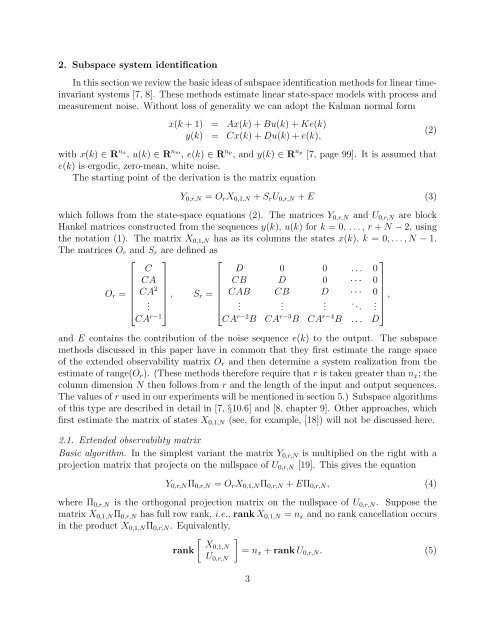
2. Subspace system identificationInthissectionwereviewthebasicideasofsubspaceidentificationmethodsforlineartimeinvariantsystems [7, 8]. These methods estimate linear state-space models with process andmeasurement noise. Without loss of generality we can adopt the Kalman normal formx(k +1) = Ax(k)+Bu(k)+Ke(k)y(k) = Cx(k)+Du(k)+e(k),(2)with x(k) ∈ R nx , u(k) ∈ R nm , e(k) ∈ R np , and y(k) ∈ R np [7, page 99]. It is assumed thate(k) is ergodic, zero-mean, white noise.The starting point of the derivation is the matrix equationY 0,r,N = O r X 0,1,N +S r U 0,r,N +E (3)which follows from the state-space equations (2). The matrices Y 0,r,N and U 0,r,N are blockHankel matrices constructed from the sequences y(k), u(k) for k = 0, ..., r +N −2, usingthe notation (1). The matrix X 0,1,N has as its columns the states x(k), k = 0,...,N − 1.The matrices O r and S r are defined as⎡ ⎤ ⎡⎤C D 0 0 ... 0CACB D 0 ··· 0O r =CA 2, S⎢ ⎥ r =CAB CB D ··· 0,⎢⎥⎣ . ⎦ ⎣ . . .... . ⎦CA r−1 CA r−2 B CA r−3 B CA r−4 B ... Dand E contains the contribution of the noise sequence e(k) to the output. The subspacemethods discussed in this paper have in common that they first estimate the range spaceof the extended observability matrix O r and then determine a system realization from theestimate of range(O r ). (These methods therefore require that r is taken greater than n x ; thecolumn dimension N then follows from r and the length of the input and output sequences.The values of r used in our experiments will be mentioned in section 5.) Subspace algorithmsof this type are described in detail in [7, §10.6] and [8, chapter 9]. Other approaches, whichfirst estimate the matrix of states X 0,1,N (see, for example, [18]) will not be discussed here.2.1. Extended observability matrixBasic algorithm. In the simplest variant the matrix Y 0,r,N is multiplied on the right with aprojection matrix that projects on the nullspace of U 0,r,N [19]. This gives the equationY 0,r,N Π 0,r,N = O r X 0,1,N Π 0,r,N +EΠ 0,r,N , (4)where Π 0,r,N is the orthogonal projection matrix on the nullspace of U 0,r,N . Suppose thematrix X 0,1,N Π 0,r,N has full row rank, i.e., rankX 0,1,N = n x and no rank cancellation occursin the product X 0,1,N Π 0,r,N . Equivalently,[ ]X0,1,Nrank = nU x +rankU 0,r,N . (5)0,r,N3