Modeling bone regeneration around endosseous implants

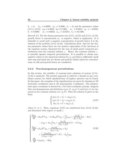
22 Chapter 2. Linear stability analysisb − = 0; m + ≈ 0.9959, s 2+ ≈ 2.3898, b + = 0; and for parameter values(2.11), (2.13): m 0 ≈ 0.3253, b 0 ≈ 8.1293; m − ≈ 0.0012, s 2− ≈ −0.0245,b − ≈ 0.0290; m + ≈ 0.6623, s 2+ ≈ 42.9271, b + ≈ 16.5486.Remark 2.5. For the chosen parameter sets (2.11), (2.12) and (2.11), (2.13),growth factor 2 concentration s 2− is negative, which is unphysical. It isdesirable to avoid such a negative concentration of growth factor 2 in thesolution of the problem (2.14)–(2.16). Calculations show, that for the chosenparameter values there are two positive eigenvalues of the Jacobean ofthe equation system, linearized for the case of small purely temporal perturbationsnear the constant solution z − . Hence, the constant solution z −is unstable against temporal perturbations. It is possible to obtain nonnegativevalues in the numerical solution for s 2 , provided a sufficiently smalltime step and mesh size are chosen and positive initial values for concentrationsof cells and growth factor are considered.2.3.2 Non-homogeneous perturbationsIn this section, the stability of constant-state solutions of system (2.14)–(2.16) is analyzed. The present approach is valid for a domain in any coordinatesystem, for which eigenfunctions of Laplace operator can be found.In this paper, the examples of the eigenfunctions are given for domains in 1DCartesian coordinates and in 1D axisymmetric coordinates. The independentspace coordinate is denoted by x for both coordinate systems. Supposethat non-homogeneous perturbations m p (x, t), s 2p (x, t) and b p (x, t) are imposedon the constant solution (m ′ , s ′ 2 , b′ ). Then the solution is given in theform:⎧⎪⎨⎪ ⎩m(x, t) = m ′ + εm p (x, t),s 2 (x, t) = s ′ 2 + εs 2p (x, t),b(x, t) = b ′ + εb p (x, t),(2.27)where |ε| ≪ 1. Then, equations (2.27) are substituted into (2.14)–(2.16),and linearized with respect to small ε:⎧⎪⎨⎪⎩∂m p∂t[(=D m ∇ 2 m p − m ′ B m2 ∇ 2 s 2p + α m0 + α ms ′ 2β m + s ′ 2]− (α p0 + A m ) m p +α mβ m(β m + s ′ 2 )2 m′ (1 − m ′ )s 2p ,∂s 2p=D s2 ∇ 2 s 2p + α m2s ′ 2∂tβ m2 + s ′ (m p + b p )2[ αm2 β]m2+(β m2 + s ′ 2 )2 (m′ + b ′ ) − A s2 s 2p ,∂b p∂t =α p0m p − A b b p .)(1 − 2m ′ )(2.28)