allan variance estimated by phase noise measurements - PTTI

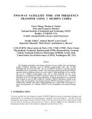
36 th Annual Precise Time and Time Interval (PTTI) Meeting 

ALLAN VARIANCE ESTIMATED BY 

PHASE NOISE MEASUREMENTS 

P. C. Chang, H. M. Peng, and S. Y. Lin 

National Standard Time & Frequency Lab., TL, Taiwan 

12, Lane 551, Min-Tsu Road, Sec. 5, Yang-Mei, Taoyuan, Taiwan 326 

Tel: 886 3 424 5179, Fax: 886 3 424 5474, E-mail: betrand@cht.com.tw 

Abstract 

For short measurement times, the Allan (or two-sample) variance can be determined from 

the phase noise using the mathematical conversion between time and frequency domain. This 

provides us with a useful tool to obtain the very short-term frequency stability (τ


FFT (Fast Fourier Transform) spectrum analyzer. The signal reference is from a SDI LNFR-400 lownoise 

frequency reference with a noise level of about –173 dBc/Hz (5 MHz PM, at Fourier frequency 100 

KHz). The system can measure up to –177 dBc/Hz for passive devices [4]. Recently, we improved the 

system using a cross-correlation technique, which enhances the measurement capability to measure the 

noise 15~20 dBc/Hz below the previous one. With Sy(f) from the phase noise measurement, getting the 

very-short-term frequency stability (τ < 0.5 sec.) in the time domain via time-frequency domain 

conversion is made possible. Adversely, it is not easy to measure the very-short-term frequency stability 

using a time-interval counter directly due to its resolution limitations. The traditional time-interval 

counter is applicable only when the sampling time τ is not smaller than 1 second. 

As for the mathematical conversion, two methods are adopted for comparison. The numerical integration, 

or trapezoidal integration to be precise, could calculate the Allan variance easily after the experimental 

data are properly processed. Besides, the power-law model is frequently used for describing the phase 

noise and it assumes that the spectral density of normalized frequency fluctuations is equal to the sum of 

terms, each of which varies as an integer power of Fourier frequency f. Thus, there are two quantities that 

completely specify Sy(f) for a particular power-law process: the slope on a log-log plot for a given range 

of f and the amplitude. The slope is denoted by α and, therefore, f α is the straight line on a log-log plot 

that relates Sy(f) to f. The amplitude is denoted by hα. Therefore, Sy(f) can be represented by the addition 

of all the power-law processes with the appropriate coefficients: 

⎧ 

⎪ 

< < 

= ⎨ 

⎪ 

⎩ 

> 

∑+ 

2 

α 

h αf 

for 0 f f h 

S y ( f ) α= 

−2 

(2) 

0 for f f h 

While 2πfhτ >> 1, Cutler derived equation (3) from equation (1) and (2): 

2 

h 1. 

038 + 3ln( 

2πf 

τ) 

σ y ( τ) 

+ 

6 

2τ 

( 2π) 

τ 

2 

( 2π) 

0 

h 

h 

= h − 2 τ + h −1 

2ln 

2 + + h1 

h 

2 2 

2 

(3) 

2 2 

By properly determining the coefficients, the Allan variance with different τ could be obtained using 

Cutler’s equation. This could be achieved by locating each particular noise process in its dominant range 

of f with standard regression techniques. 

II. TESTS OF FIVE NOISE TYPES 

Before carrying out the mathematical conversion using the experimental results, we would like to know 

how each noise process behaves in this conversion. According to the power-law model, there are five 

types of noise processes, including Random Walk FM, Flicker FM, White FM, Flicker PM and White PM, 

with α equal to -2, -1, 0, +1, and +2 respectively. That means we need to generate five different Sy(f) for 

tests. For example, Sy(f) of the Random Walk FM noise process could be obtained by assuming the 

amplitude coefficient h-2 equal to 1×10 -26 with the rest equal to zero. The numerical integration and the 

power-law model are then used to calculate the Allan deviation (ADEV), that is, the square root of the 

Allan variance. With τ ranging from 1 millisecond to 10 seconds, the calculated ADEVs from both 

methods are shown in Figure 1 (a). It is obvious that while τ is smaller than 1 second, their ADEVs are in 

good agreement with each other. In this manner, Sy(f) of the other noise processes can be generated by 

separately assuming h-1 = 1×10 -26 , h0 = 1×10 -26 , h+1 = 4×10 -28 , and h+2 = 3×10 -31 for the corresponding noise 

processes and their ADEVs are shown in Figure 1 (b), (c), (d), and (e). 

166 

3f 

( 2π) 

τ


It can be seen that for the noise processes of Flicker FM and White FM, the ADEV from both methods 

are in good agreement with each other while τ is smaller than 1 second; for Flicker PM, the ADEV from 

both methods match each other well in the whole range of τ, but for white PM, the results using the 

numerical integration vary up and down depending on τ, while the ones using the power-law model do 

not. Furthermore, only for some certain values of τ would the ADEV from both methods match each 

other well as to the last noise process. 

(a) 

(c) 

(e) 

Figure 1. The ADEV of five types of noise processes using the numerical 

integration and the power-law model. The sampling time τ is from 1 

millisecond to 10 seconds. 

167 

(b) 

(d)


III. RESULTS AND CALCULATIONS 

Realizing how each individual noise process behaves in the conversion using these two methods, we try 

to convert the real phase noise measurement data into ADEV. Here we take the noise floor of our 

measurement system to be an example. A 5 MHz reference signal is split with a reactive splitter to 

provide a pair of input signals. These signals are connected to the LO and RF ports of a double-balanced 

mixer. A delay line unit is required here to put the two signals into quadrature (90° out of phase) before 

entering the mixer. The output of the mixer is low pass filtered, amplified, and then fed into a FFT 

spectrum analyzer. 

The spectral density of the system noise floor is shown in the upper graph of Figure 2. The Fourier 

frequency range is from 0.12 Hz to 99.75 kHz. There are some spur-like components appearing 

obviously in the graph, like noises of 60 Hz, 120 Hz, 180 Hz, etc. It is clear that most of the outliers 

should arise from the ac power noise, which is always inevitably getting into the measurement system or 

the DUT. In order to check how much these spur-like components influence the calculation of the ADEV, 

we use the raw data and the outliers-removed data to calculate the ADEV and then compare them. The 

corrected spectral density of the system noise floor is shown in the lower graph of Figure 2. 

Figure 2. Spectral density of the system noise floor in Fourier frequency 

ranging from 0.12 Hz to 99.75 kHz. Upper graph: Spectral density consisting 

of spur-like periodic noises, e.g. ac power noise. Lower graph: Outliers are 

removed from the spectral density. 

The measure L (f) on the y-axis is the prevailing expression of the phase noise among manufacturers and 

users of frequency standards. Its relation to Sy(f) can be expressed as: 

168

(4) 


1 1 v0 

( f ) = Sφ 

( f ) = ( S 2 

2 2 f 

L y 

169 

2 

( f )) 

Sφ(f) is the spectral density of phase fluctuations and v0 is the carrier frequency. L (f) is usually reported 

in a dB format. 

dBc 

= 10 log ( L ( f )) 

Hz 

(5) 

After some calculations, the results from above-mentioned data using the numerical integration are shown 

in Figure 3. Roughly speaking, the spur-like components make the generated ADEV bigger than the 

other one, but because both of them vary up and down inconsistently, depending on τ, it is hard to 

precisely identify how much these spur-like components contribute to the ADEV. 

Figure 3. The ADEV calculated from the raw data with spur-like components and the 

outliers-removed data using the numerical integration. Both of them vary up and 

down inconsistently, depending on τ. 

The power-law model is not applicable here because the existence of spur-like components is not in its 

basic assumption. It is meaningless to fit the experimental data with the model. Nevertheless, we can 

still make the ADEV comparison with the outliers-removed data using the numerical integration and 

power-law model. In the lower graph of Figure 2, we see that when f increases by one decade, L (f) also 

goes down by one decade for f = 0.12 ~ 1000 Hz. The dominant noise process in this range can be 

regarded as Flicker PM. For f = 10 ~ 99.75 kHz, L (f) is almost the same, and the dominant noise process 

should be White PM. We use the functions h+1f and h+2f 2 to fit the data in the corresponding range and 

get h+1 = 4.68 × 10 -28 and h+2 = 2.61 × 10 -31 . With the help of Cutler’s equation, we can compare the 

generated ADEV with the one using the numerical integration, as shown in Figure 4.


We observe that the results using the numerical integration vary up and down, depending on τ, while the 

ones using the power-law model do not. Furthermore, only for some certain values of τ would the ADEV 

from both methods match each other well. Since there are only two noise processes existent in the data, it 

seems to be a reasonable conclusion that the noise process of White PM in the data should be responsible 

for this observation, as shown in the previous tests of five noise types. 

Figure 4. The ADEV calculated from the outliers-removed data using the numerical 

integration and the power-law model. The former varies up and down, depending on 

τ, while the latter does not. 

IV. CONCLUSIONS 

In this paper, we use the phase noise data in our lab to calculate the ADEV via the time-frequency domain 

conversion. The numerical integration and Cutler’s equation derived from the power-law model are two 

methods adopted for comparison. We observe that for the noise processes of Random Walk FM, Flicker 

FM, White FM, and Flicker PM, the ADEV from both methods match each other well while τ is smaller 

than 1 second, but for White PM, the ADEV using the numerical integration varies up and down, 

depending on τ, while the one using the power-law model does not. This observation is shown both in the 

individual noise tests and the result from a real phase noise measurement. That means obtaining the veryshort-term 

frequency stability (τ < 0.5 second) in the time domain is possible if the discrepancy of the 

White PM calculation from the two methods can be resolved. Besides, as for the influence of ac power 

noise, it is hard to precisely identify how much these spur-like components contribute to the ADEV, also 

due to the influence of White PM using the numerical integration. In order to solve this problem, we will 

do more research in the near future. 

REFERENCES 

[1] Samuel R. Stein, 1985, “Frequency and Time - Their Measurement and Characterization,” Precision 

Frequency Control, Vol. 2, Chap. 12, pp. 203-204. 

170


[2] “Characterization of Frequency and Phase Noise,” Report 580 of the International Radio 

Consultative Committee (C.C.I.R), pp. 142-150, 1986. 

[3] D. Allan, H. Hellwig, P. Kartaschoff, J. Vanier, J. Vig, G. M. R. Winkler, and N. Yannoni, 1988, 

“Standard Terminology for Fundamental Frequency and Time Metrology,” in Proceedings of the 

42 nd Annual Symposium on Frequency Control, 1-3 June 1988, Baltimore, Maryland, USA (IEEE 

88CH2588-2), pp. 419-425. 

[4] Femtosecond Systems, Inc., FSS1000E Phase Noise Detector FSS1011A Delay Line Operation 

Manual, Chap. 1. 

171


QUESTIONS AND ANSWERS 

SAM STEIN (Timing Solutions Corporation): I am confused about the outliers. What is the nature of 

the outliers? 

PO-CHENG CHANG: They are the AC power influence. 

STEIN: They are dispersed? 

CHANG: Yes. 

172

allan variance estimated by phase noise measurements - PTTI

You also want an ePaper? Increase the reach of your titles

Delete template?

Save as template?