PhD thesis in English

UNIVERSITY OF BELGRADEFACULTY OF PHYSICSIvana B. VidanovićNUMERICAL STUDY OF QUANTUMGASES AT LOW TEMPERATURESDoctoral DissertationBelgrade, 2011

UNIVERZITET U BEOGRADUFIZIČKI FAKULTETIvana B. VidanovićNUMERIČKO PROUČAVANJE KVANTNIHGASOVA NA NISKIM TEMPERATURAMADoktorska disertacijaBeograd, 2011

Thesis advisor, Committee member:Dr. Antun BalažAssociate Research ProfessorInstitute of Physics BelgradeUniversity of BelgradeCommittee member:Dr. Aleksandar BogojevićAssociate Research ProfessorInstitute of Physics BelgradeUniversity of BelgradeCommittee member:Prof. Dr. Sunčica Elezović-HadžićAssociate ProfessorFaculty of PhysicsUniversity of BelgradeCommittee member:Prof. Dr. Milan KneževićProfessorFaculty of PhysicsUniversity of BelgradeThe doctoral dissertation of Ivana Vidanović was defended on December 23, 2011.

Dedicated to the memory of my father, Bora Vidanović.

lence for Computer Modeling of Complex Systems). Numerical simulationswere run on the AEGIS e-Infrastructure, supported in part by theEuropean Commission under EU FP7 projects PRACE-1IP, HP-SEEand EGI-InSPIRE.Finally, I am indebted to my mother, sister and Borislav for their unwaveringsupport that goes far beyond my graduate studies.

Rezime doktorske disertacijeNumeričko proučavanje kvantnih gasovana niskim temperaturamaKoncept Boze-Ajnštajn kondenzacije je u fizici prisutan još od 1924. godine, kadaje prvi put uvedena Boze-Ajnštajn statistika za identične čestice celobrojnog spina[1, 2]. Već prva teorijska kvantno-mehanička razmatranja sistema neinteragujućihčestica su ukazala na mogućnost postojanja ovog fenomena. Poznato je da fizičkeosobine atomskih gasova jako zavise od temperature. Na sobnim temperaturama,osobine ovih sistema su dobro opisane zakonima klasične statističke fizike i kvantnifenomeni prolaze neopaženo. Snižavanjem temperature talasna dužina de Broljijevihtalasa materije raste i dolazi do preklapanja talasa koji odgovaraju različitimčesticama. U tom slučaju, kvantna statistika preuzima presudnu ulogu za fizičke osobinesistema. Česticama sa celobrojnim spinom, bozonima, zakoni kvantne statistikedozvoljavaju naseljavanje istog jednočestičnog kvantnog stanja. Kako snižavamotemperaturu, sistem teži konfiguraciji sa minimalnom energijom, a za bozone to jeupravo makroskopski naseljeno osnovno kvantno stanje. Na taj način ovo kvantnostanje postaje dominantno, pa govorimo o makroskopskom kvantnom fenomenu irazlikujemo fazu sa makroskopskom naseljenošću osnovnog stanja (Boze-Ajnštajnkondenzat) i fazu bez ovog svojstava, koju nazivamo normalni gas. Fazni prelazizmedu ove dve faze naziva se Boze-Ajnštajn kondenzacija. I pored jake utemeljenostiteorijskog koncepta, do prve eksperimentalne realizacije ovog faznog prelaza jedošlo tek 1995. godine, a rezultat je nagraden Nobelovom nagradom za fiziku 2001.Kao što smo ukratko objasnili, osnovni pojmovi o fenomenu Boze-Ajnštajn kondenzacijesu uvedeni korišćenjem modela neinteragujućeg gasa. U realnim gasovimaje naravno nemoguće zanemariti interakcije, zbog kojih oni na veoma niskim temperaturamaprelaze u tečno ili čvrsto stanje. Zbog toga je za eksperimentalno postizanjeBoze-Ajnštajn faznog prelaza neophodno koristiti slabo interagujuće gasove,kao što su su, na primer, razredeni gasovi koji interaguju kratkodometnom, Vander-Valsovominterakcijom. U takvom sistemu, u kom je srednje rastojanje izmedučestica veliko zbog male gustine, kvantni fenomeni dolaze do izražaja tek na veomaniskim temperaturama. Zbog mogućnosti efikasnog hladenja, za eksperimentalno

dobijanje kondenzata odabrani su atomski gasovi alkalnih metala (Rb, Li, Na, ...), ukojima je fenomen Boze-Ajnštajn kondenzacije i ostvaren po prvi put [3, 4] za tipičnegustine čestica u opsegu od 10 18 m −3 do 10 21 m −3 (što je šest redova veličine manjeod tipične gustine vazduha) i temperature reda 100 nK. Postizanje ovako niskihtemperatura je zahtevalo razvijanje novih tehnika hladenja i čuvanja atoma, koji suu eksperimentu zarobljeni u zamci napravljenoj od specijalno podešenog spoljašnjegelektričnog ili magnetnog polja. Posle intenzivnih dugogodišnjih napora, proizvodnjakvantnih gasova sačinjenih od raznih vrsta alkalnih atoma je danas standardniproces u brojnim laboratorijama širom sveta.Eksperimenti omogućavaju veoma detaljno testiranje fundamentalnih teorijskihkoncepata - kolektivnih ekscitacija Boze-Ajnštajn kondenzata, superfluidnosti (prisustvovorteksa kao odgovor sistema na spoljašnju rotaciju), osobina faznog dijagrama[5]. Veoma važna i interesantna osobina ultrahladnih kvantnih gasova jeekstremno velika mogućnost kontrole svih relevantnih parametara sistema - brojačestica, gustine, temperature, dimenzionalnosti (promenom oblika spoljašnje potencijalnezamke), a posebno je značajna mogućnost kontrolisanja jačine interakcijaizmedu atoma tehnikom koja se naziva Fešbah rezonanca [6]. Jednostavnompromenom spoljašnjeg magnetnog polja, efektivna interakcija izmedu atoma se možemenjati u rasponu od mnogo redova veličina, što čini ove sisteme zaista jedinstvenim.U novijim eksperimentima, atomi su zarobljeni u periodičnim potencijalima, tzv.optičkim rešetkama [7]. Zahvaljujući tome, sada je moguće na nov način realizovatii proučavati sisteme koji su analogni sistemima poznatim iz fizike čvrstogstanja, a koje još uvek ne razumemo u potpunosti (npr. visoko-temperaturna superprovodljivost).Upravo zato se kaže da ultrahladni kvantni gasovi predstavljajuFajnmanove “kvantne simulatore” [8]. Intenzivan eksperimentalni razvoj i realizacijanove ultrahladne faze materije predstavljaju snažan podsticaj za nova, interdisciplinarnateorijska istraživanja.Osnovni cilj ove teze je podrobno razumevanje dva zanimljiva fizička scenarijaza manipulaciju hladnim bozonskim atomima, koja su predmet i nedavnih eksperimentalnihistraživanja. Prvo smo razmotrili fazni dijagram rotirajućeg idealnogbozonskog gasa u anharmonijskom potencijalu, dok se druga noseća tema teze bavinelinearnim osobinama kolektivnih bozonskih moda, koje su pobudene harmonijskommodulacijom interakcije.Da bismo ostvarili ove ciljeve, najpre smo u Poglavlju 2 razradili detalje numeričkogmetoda koji nam na efikasan način pruža informaciju o velikom broju

svojstvenih stanja kvantnog sistema. Tačno poznavanje energetskih nivoa nam jeneophodno radi preciznog odredivanja faznog dijagrama Boze-Ajnštajn kondenzata.Metod koji smo koristili je zasnovan na egzaktnoj dijagonalizaciji evolucionog operatora[9], a da bi postigli njegovu optimalnu upotrebu, detaljno smo analiziraligreške koje nastaju pri korišćenju ovog metoda iz dva razloga: greške nastale usleduvodenja prostorne diskretizacije, kao i greške pri računanju matričnih elemenataevolucionog operatora. Jedan od naših glavnih rezultata je mnogo optimalnijeponašanje diskretizacione greške ovog metoda u odnosu na standardni metod dijagonalizacijeprostorno diskretizovanog Hamiltonijana. Detaljnim analitičkim inumeričkim razmatranjem, pokazali smo da dijagonalizacija diskretizovanog evolucionogoperatora pokazuje neperturbativno malu diskretizacionu grešku, koja opadaeksponencijalno sa 1/∆ 2 , gde je ∆ korak prostorne diskretizacije, dok standardnimetodi imaju grešku koja polinomijalno zavisi od ∆. Ovo je osnovni razlog zbogkog je mnogo optimalnije koristiti dijagonalizaciju evolucionog operatora. Glavnateškoća u primeni ovog pristupa - precizno računanje matričnih elemanata evolucionogoperatora, tj. amplituda prelaza, direktno se razrešava primenom ranije uvedenogmetoda efektivnih dejstava [10, 11], koja nam daju razvoj amplitude prelazapo kratkom vremenu propagacije do veoma visokog nivoa. Veliku efikasnost ovogmetoda smo demonstrirali na nekoliko jednodimenzionalnih i dvodimenzionalnihmodela.U poglavlju 3 primenili smo prethodno opisani metod na ispitivanje faznogdijagrama rotirajućih bozona u nestandardnom spoljašnjem potencijalu. Naime,najčešće korišćene potencijalne zamke su harmonijskog oblika, i o Boze-Ajnštajnkondenzaciji u ovakvim zamkama se već puno zna. Rotacija kvantnog gasa je jedanod načina da se ostvare jako korelisane faze materije [7] i od velikog je značaja.Medutim, jedna od posledica rotacije je pojava dekonfinirajuće centrifugalne komponenteu potencijalu, koja za velike frekvencije rotacije (veće of frekvencije harmonijskepotencijalne zamke) dovodi do razletanja čestica gasa i gubitka kondenzata.Da bi se to izbeglo, u nedavnom eksperimentu [12] je upotrebljen dodatnikvartični potencijal za formiranje potencijalne zamke. U zavisnosti od frekvencijerotacije, ukupan efektivni potencijal menja oblik od konveksnog potencijala sa jednimminimumom do potencijala koji ima oblik meksičkog šešira. Primenom egzaktnedijagonalizacije evolucionog operatora, proučavali smo kako promena spoljašnjeg potencijalautiče na temperaturu Boze-Ajnštajn kondenzacije, na raspodelu čestica uzamci i na rezultate eksperimentalnih merenja.

Uticaj slabih interakcija na fenomen Boze-Ajnštajn kondenzacije je predmet razmatranjaPoglavlja 4. Ovo poglavlje je preglednog tipa, i u njemu smo predstaviliHartri-Fok opis bozonskog sistema. Hartri-Fok predstavlja jednu od aproksimacija uteoriji srednjeg polja, i u okviru nje smo opisali sistem ultrahladnih bozona na nultojtemperaturi, kao i u okolini Boze-Ajnštajn faznog prelaza. Za nultu temperaturusmo izveli čuvenu Gros-Pitaevski jednačinu [13, 14] - nelinearnu parcijalnu diferencijalnujednačinu koja opisuje ponašanje makroskopse talasne funkcije kondnezata.Za konačne temperature predstavili smo nekoliko često korišćenih implementacijaaproksimacije srednjeg polja i naveli njihove prednosti i nedostatke. Aproksimativnimetodi ove vrste se veoma često koriste u interpretaciji eksperimentalnih merenja,što im daje veliki značaj. Nedavni eksperimentalni napredak u uočavanju efekatakoji su izvan opisa teorije srednjeg polja zahteva popravke standardno korišćenihaproksimacija u najskorijoj budućnosti.Jedan od osnovnih načina karaketrizacije faza materije, kako eksperimentalnotako i teorijski, su osobine njihovog ekscitaciong spektra, a posebno su interesantnei važne kolektivne mode. U sistemima hladnih gasova, kolektivne mode se običnopobuduju modulacijom spoljašnjeg potencijala zamke, dok je u nedavnom eksperimentalnomradu [15] pobudivanje kolektivnih moda ostvareno novim pristupom- harmonijskom modulacijom interakcije. U osnovi primenjenog eksperimentalnogmetoda je tehnika Fešbah rezonance, kojom se jačina kratkodometne interakcijemenja u vremenu usled modulacije spoljašnjeg magnetnog polja. Kao posledicu,imamo oscilacije veličine bozonskog oblaka, koje su u eksperimentu merene. U zavisnostiod vrednosti spoljašnje frekvencije upotrebljene za modulaciju interakcije,možemo da dobijemo linearni odgovor sistema ili rezonantno ponašanje karakterisanovelikim amplitudama oscilacija. Kako je osnovna jednačina koja opisuje dinamikuovakvog sistema nelinearna, u slučaju velikih oscilacija očekujemo izraženenelinearne efekte. U poglavlju 5 smo numerički simulirali dinamiku sistema i identifikovalinelinearne karakteristike dobijenih ekscitacionih spektara: pored osnovnihmoda, pojavljuju se viši harmonici, kao i linearne kombinacije različitih moda, anajizraženiji nelinearni efekati su pomeraji u frekvencijama ekscitovanih moda uodnosu na vrednosti izračunate u linearnom režimu. Za kvantitativno objašnjenjenelinearnih efekata razvili smo perturbativi pristup u kom je mali parametar amplitudamodulacije. Razvijeni perturbativni pristup je baziran na Poenkare-Lindštetmetodu, i njegovom primenom smo našli analitičke izraze za nelinearne pomerajesvojstvenih frekvencija u blizini rezonanci.

Ključne reči: hladni kvantni gasovi, Boze-Ajnštajn kondenzacija, efektivnodejstvo, egzaktna dijagonalizacija, teorija perturbacija, nelinearna dinamikaNaučna oblast: FizikaUža naučna oblast: Fizika kondenzovanog stanja materijeUDK broj: 538.9

Abstract of the doctoral dissertationNumerical study of quantum gasesat low temperaturesThe concept of Bose-Einstein condensation was introduced in 1924, at the sametime as Bose-Einstein statistics, applicable to the integer-spin particles [1, 2]. Alreadyfirst theoretical quantum-mechanical considerations pointed to the existence ofthis phenomenon. It is well known that physical properties of atomic gases stronglydepend on the temperature. At room temperatures the properties of these systemscan be described by the classical statistical physics, and quantum features are negligible.However, as the temperature decreases, the wavelengths of the de Brogliemater waves increase, leading to the overlap of waves corresponding to different particles.In this case, quantum statistics plays a dominant role. According to the rulesof quantum statistics, integer-spin particles, bosons, are allowed to occupy the samesingle-particle quantum states. With the decrease in the temperature, the systemseeks the minimal-energy configuration, and for bosons this is a macroscopicallyoccupied single-particle ground state. Such a quantum state becomes dominant andthe occurrence is designated as a macroscopic quantum phenomenon. Accordingly,we distinguish a phase with a macroscopic occupation of the ground state (Bose-Einstein condensate) and a phase without this feature, which is called a normal gas.The phase transition between the two phases is Bose-Einstein condensation. In spiteof the firm theoretical foundation of the concept from the beginning, first direct experimentalobservation was achieved only in 1995, and the result was recognized bythe Nobel prize for physics in 2001.As briefly explained, the basic notion of Bose-Einstein condensation was introducedusing a model of noninteracting gas. Of course, in realistic gases, interactionscan not be neglected and only due to them the gas becomes liquid or solid at lowtemperatures. In order to remain close to the noninteracting gas description inexperiments, it is essential to use weakly interacting gases, such as dilute gases interactingvia short-range, van der Waals interaction. In this type of systems, withlong interparticle distances due to diluteness, the quantum phenomena become relevantonly at very low temperatures. Due to highly efficient cooling techniques,

the gases of alkali metals (Rb, Li, Na, ...) were selected as most suitable candidatesand Bose-Einstein condensation was observed for the first time [3, 4] in such systemswith the typical particle densities from 10 18 m −3 to 10 21 m −3 (six orders of magnitudelower than the density of air) and temperatures of the order of 100 nK. In order toreach this extreme low-temperature regime, it was necessary to develop many newcooling and trapping techniques: in experiments, atoms are confined using speciallydesigned configurations of external magnetic or electric fields. After many yearsof intensive experimental efforts, the achievement of Bose-Einstein condensation incold alkali vapors is nowadays a common technique in laboratories all over the world.The experiments make possible very detailed tests of fundamental theoreticalconcepts - collective excitations of a Bose-Einstein condensate, superfluidity (theappearance of vortices as a response to rotation), the properties of a phase diagram[5]. A very important and interesting feature of ultracold quantum gases is a possibilityto control relevant parameters of the system over many orders of magnitude.Basically, all parameters can be tuned: number of particles, density, temperature,dimensionality (by changing the shape of the external trap), and even the strengthof interactions between atoms using a technique called Feshbach resonance [6]. Bya simple modification of the external magnetic field, the effective interatomic interactioncan be tuned in the range of several orders of magnitude and this featuremakes cold atomic systems really unique. In more recent experiments, atoms aretrapped in periodic potentials, the so-called optical lattices [7]. In this way, it isnow possible to study, in a very clean setup, systems which are highly relevant incondensed matter physics, and which are not yet completely understood (with a notableexample of high-temperature superconductivity). For this reason, it is widelyaccepted that ultracold quantum gases represent Feynman’s quantum simulators [8].Intensive experimental progress and realization of the new ultracold phase of matterare strong stimuluses for further, interdisciplinary theoretical research.The main subject of this thesis is a thorough understanding of two interestingphysical scenarios for the manipulation of cold bosonic atoms, which were also thefocus of recent experimental studies. First, we have explored the phase diagram ofa rotating ideal bosonic gas in an anharmonic trap, while the second main topicdeals with nonlinear features of collective modes excited by harmonic modulation ofinteraction strength.On the way to accomplish this, after introductory Chapter 1, in Chapter 2 wehave first worked out details of an efficient numerical method capable of providing

highly accurate information on energy levels of quantum systems. The precise informationon energy spectra is necessary for the characterization of the phase diagramof a Bose-Einstein condensate. Method that we have used is based on the exactdiagonalization of the time-evolution operator [9]. In order to optimally apply it,we have carefully analyzed numerical errors which arise for two reasons: numericalerrors which stem from the spatial discretization, as well as the errors due tothe approximative calculation of matrix elements. One of our main results is highlysuperior behavior of the dicretization error of the discretized evolution operator comparedto the common discretization error of the discretized Hamiltonian. Based onthe analytical and numerical considerations, we have shown that the diagonalizationof a time-evolution operator exhibits a non-perturbatively small discretization error,which vanishes exponentially with 1/∆ 2 , where ∆ is the discretization spacing,while standard discretization introduces errors polynomial in ∆. This is the mainreason that makes the diagonalization of the time-evolution operator the preferredmethod. The main difficulty in the application of the method - precise calculationof the matrix elements of time-evolution operator (transition amplitudes) can be directlyresolved using previously developed effective action approach [10, 11], whichyields transition amplitudes as high-order expansions in the short time of propagation.The efficiency of this method has been demonstrated on several one- andtwo-dimensional models.In Chapter 3 we have used the described numerical method to explore the phasediagram of rotating bosons in a non-standard external potential. Widely used confinementsare harmonic traps and many details of Bose-Einstein condensation insuch traps are already well understood. Rotation of a quantum gas is one way toreach strongly correlated phases [7] and is therefore highly relevant. One of the consequencesof rotation is the appearance of the deconfining centrifugal component inthe potential, which in the case of a very fast rotation frequency (exceeding the trappingfrequency) leads to the deconfinement. In order to avoid this, recent experiment[12] introduced an additional quartic potential to enhance trapping. Depending onthe value of the rotation frequency, the potential changes its shape from a simpleconvex one to the Mexican-hat-shaped potential. Using exact diagonalization of thetime-evolution operator, we have studied how the modification of the external trapinfluences properties of a Bose-Einstein condensate, such as condensation temperature,equilibrium density distribution of atoms and the expansion time of the cloudafter it is released from the trap.

The effects of weak interactions on the phenomenon of Bose-Einstein condensationare subject of Chapter 4. This chapter reviews the Hartree-Fock descriptionof a bosonic system. Hartree-Fock is one of the mean-field approximations andwithin this framework we have described ultracold bosons at zero temperature, aswell as in the vicinity of the Bose-Einstein phase transition. At zero temperaturewe have rederived famous Gross-Pitaevskii equation [13, 14] - nonlinear partial differentialequation, which governs the dynamics of the macroscopic wave functionof the condensate. For finite temperatures, we have scrutinized several widely usedimplementations of the mean-field approximation, with the emphasis on their benefitsand their physical drawbacks. Approximations of this type are very often usedin the interpretation of the experimental data, which makes them highly relevant.A very recent experimental progress in the observation of beyond-mean-field effectsdemands further improvements of these standard tools.One of the basic methods to characterize phases of matter, both experimentallyand theoretically, are properties of their excitation spectra, with collective modesbeing of special interest. In ultracold gases, collective modes are usually excited usingmodulation of the parameters of the external trap. In the recent experiment [15],however collective modes were excited using an alternative method - harmonic modulationof interaction. In its essence the experimental method relies on a Feshbachresonancetechnique, which enables modulation of interaction via a modulation ofthe external magnetic field. As an outcome of this dynamical protocol, oscillationsof the condensate size were induced and measured. Depending on the value of theexternal modulation frequency, either a linear response or resonant large-amplitudeoscillations were obtained. Since the main underlying equation is nonlinear, in thecase of large-amplitude oscillations strong nonlinear effects are expected. In Chapter5 we have performed numerical simulations of the system dynamics and identifiedmain nonlinear features of the obtained excitation spectra: beside the basic modes,higher harmonics appear together with their linear combinations. Most prominentnonlinear effects are nonlinearity-induced shifts in the frequencies of excited modes.In order to describe these results in an analytic way, we have developed perturbativeapproach where the small parameter is given by the modulation amplitude.The developed perturbative approach is based on the Poincaré-Lindstedt method,and gives analytical estimates for the shifts of the eigenfrequencies in the vicinity ofresonances.

Keywords: cold quantum gases, Bose-Einstein condensation, effectiveaction, exact diagonalization, perturbation theory, nonlinear dynamicsField of Science: PhysicsResearch Area: Condensed matter physicsUDC number: 538.9

ContentsNomenclaturexviii1 Introduction 11.1 Foreword . . . . . . . . . . . . . . . . . . . . . . . . . . . . . . . . . . 11.2 Few basic facts on Bose-Einstein condensation . . . . . . . . . . . . . 31.2.1 Noninteracting bosonic gas in the harmonic trap . . . . . . . . 31.2.2 Experimental realization . . . . . . . . . . . . . . . . . . . . . 91.2.3 Interacting bosons at low temperatures . . . . . . . . . . . . . 131.3 This thesis . . . . . . . . . . . . . . . . . . . . . . . . . . . . . . . . . 162 Properties of quantum systems viadiagonalization of transition amplitudes 192.1 Space-discretized Schrödinger equation . . . . . . . . . . . . . . . . . 222.2 Discretization effects . . . . . . . . . . . . . . . . . . . . . . . . . . . 262.3 Effective actions . . . . . . . . . . . . . . . . . . . . . . . . . . . . . . 332.4 Numerical results for one-dimensional models . . . . . . . . . . . . . 362.5 Numerical results for two-dimensional models . . . . . . . . . . . . . 472.6 Conclusions and outlook . . . . . . . . . . . . . . . . . . . . . . . . . 553 Thermodynamics of a rotating ideal BEC 573.1 Numerical calculation of energy eigenvalues and eigenstates . . . . . . 623.2 Finite number of energy eigenvalues and semiclassical corrections . . 663.3 Global properties of rotating BECs . . . . . . . . . . . . . . . . . . . 703.3.1 Condensation temperature . . . . . . . . . . . . . . . . . . . . 703.3.2 Ground-state occupancy . . . . . . . . . . . . . . . . . . . . . 743.3.3 Comparison with semiclassical approximation . . . . . . . . . 753.4 Local properties of rotating BECs . . . . . . . . . . . . . . . . . . . . 773.4.1 Density profiles . . . . . . . . . . . . . . . . . . . . . . . . . . 77xv

CONTENTS3.4.2 Time-of-flight graphs for BECs . . . . . . . . . . . . . . . . . 793.4.3 Overcritical rotation . . . . . . . . . . . . . . . . . . . . . . . 803.5 Conclusions and outlook . . . . . . . . . . . . . . . . . . . . . . . . . 824 Mean-field description of an interacting BEC 844.1 Gross-Pitaevskii equation . . . . . . . . . . . . . . . . . . . . . . . . . 884.2 Finite-temperature properties of a BEC . . . . . . . . . . . . . . . . . 904.2.1 Almost-ideal model . . . . . . . . . . . . . . . . . . . . . . . . 914.2.2 Semi-ideal model . . . . . . . . . . . . . . . . . . . . . . . . . 924.2.3 TFSC model . . . . . . . . . . . . . . . . . . . . . . . . . . . 944.2.4 GPSC model . . . . . . . . . . . . . . . . . . . . . . . . . . . 954.2.5 Calculation of the condensation temperature . . . . . . . . . . 974.3 Experimental assessment of different models . . . . . . . . . . . . . . 1004.4 Conclusions and outlook . . . . . . . . . . . . . . . . . . . . . . . . . 1025 Nonlinear BEC dynamics by harmonicmodulation of s-wave scattering length 1045.1 Variational description of low-lying modes . . . . . . . . . . . . . . . 1075.2 Harmonic modulation of the s-wave scattering length: experiment . . 1115.3 Harmonic modulation of the s-wave scattering length:theoretical framework . . . . . . . . . . . . . . . . . . . . . . . . . . . 1145.4 Spherically-symmetric BEC . . . . . . . . . . . . . . . . . . . . . . . 1175.4.1 Poincaré-Lindstedt method . . . . . . . . . . . . . . . . . . . . 1215.4.2 Results and discussion . . . . . . . . . . . . . . . . . . . . . . 1235.5 Axially-symmetric BEC . . . . . . . . . . . . . . . . . . . . . . . . . 1265.5.1 Poincaré-Lindstedt method . . . . . . . . . . . . . . . . . . . . 1265.5.2 Results and discussion . . . . . . . . . . . . . . . . . . . . . . 1295.6 Conclusions and outlook . . . . . . . . . . . . . . . . . . . . . . . . . 1326 Summary 134A Numerical solution of the GP equation 137B Time-dependent variational analysis 142List of papers by Ivana Vidanović 144xvi

CONTENTSReferences 146CURRICULUM VITAE - Ivana Vidanović 158xvii

NomenclatureRoman Symbolsagk BLMNn(⃗r)N 0s-wave scattering lengthinteraction strength given by 4π 2 a/MBoltzmann constantspace cutoffatomic masstotal number of particlestotal density of particlesnumber of particles in the condensaten 0 (⃗r) condensate densityN thnumber of thermal particlesn th (⃗r) density of thermal particlesTtT 0 ctemperaturetimecondensation temperature of ideal gasV (⃗r) external trap potentialGreek Symbolsβinverse temperature, 1/k B Txviii

CONTENTS∆λ Tdiscretization spacingthermal de Broglie wavelength at temperature Tµ chemical potentialω x,y,ztrapping frequencyψ(⃗r) condensate wavefunctionOther SymbolsPlanck constant divided by 2πB n (µ, T) Bose-Einstein distribution⃗p⃗rmomentumreal-space coordinateAcronymsBEC Bose-Einstein condensateGPHFTFGross-PitaevskiiHartree-FockThomas-FermiTOF time-of-flightxix

Chapter 1Introduction1.1 ForewordThe essential ingredients of the quantum mechanical theory are dual particle-wavenature of the matter, and the notion of identical particles. The quantum indistinguishabilityof particles has a profound impact on the statistical properties. Whileparticles with a half-integer spin (fermions) try to avoid each other due to the Pauliexclusionprinciple, particles with an integer spin (bosons) do not exhibit such restrictionsand are actually, as a consequence of the minimal energy principle, tryingto occupy the same single-particle ground state. These effects are captured by twodifferent probability distributions that describe the thermal equilibrium in the twotypes of physical systems. The Fermi-Dirac distribution for fermions was originallyderived in 1926 by its two authors independently, while trying to introduce quantizationconcepts into an ideal gas of particles obeying the Pauli exclusion principle.The Bose-Einstein distribution for bosons was introduced in 1924 by the joint effortof Bose and Einstein [1, 2]. At the time, it was a missing piece of knowledge for thecomplete explanation of the Planck’s law of black body radiation.In the high-temperature limit, both distributions are well approximated by acommon Maxwell-Boltzmann distribution. The condition necessary for the effectsof the quantum statistics to become observable can be roughly estimated as follows.The noninteracting particles of the mass M affect each other if their thermal deBroglie wavelength λ T at temperature T,√2πλ T =2k B TM , (1.1)is comparable to the inter-particle distance given by n −1/3 , where n is a typical particledensity. Naturally, the notion of the “high temperature” and “low temperature”depends on the features of the considered system. For example, electrons in a typical1

metal at room temperature (300K) are quite accurately described by the Fermi-Diracdistribution, making the Fermi-Dirac statistics widely present in our everyday experience.Originally, the Bose-Einstein statistics was developed for the photons.Immediately after it was derived it was suggested that in the low-temperature limita macroscopic occupation of the single-particle ground state should emerge. A phaseexhibiting the macroscopic quantum phenomenon is denoted as the Bose-Einsteincondensate (BEC). An important necessity for the system to develop this type ofbehavior is the conservation of a number of particles, and as the photons can bespontaneously created and annihilated, a BEC doesn’t appear in this type of a system.Although the concept of a BEC arises at the essential level of the theory, itmanaged to escape our clear observation until the first breakthrough experiments in1995 [3, 4]. Between 1924 and 1995 a BEC was mainly discussed in the relation tothe fascinating low-temperature phenomena of superfluidity and superconductivitythat include macroscopic quantum effects. On the other hand, sometimes it waseven considered as an artifact of a noninteracting description of a bosonic gas.To explain why the concept of a BEC may seem elusive, we elaborate on stringentrequirements which are prerequisites to experimentally accomplish Bose-Einsteincondensation. As already discussed, two relevant length scales are the de Brogliewavelength and the inter-particle distance. For the first scale to be large enough,in experiments we need light particles at low temperatures. To make the secondlength scale comparable to λ T , the system of particles should be dense enough.However, the upper limit of the density is set by a requirement to remain close tothe noninteracting gas description. Strong interactions could spoil the observationof a BEC phenomena, by modifying the ground-state of the system significantly.It is well known that at low temperatures most of the elements are in the solid orliquid state, thus the noninteracting gas description loses its relevance. Eventually,experiments [3, 16] reached the regime of a dilute weakly interacting gas of alkaliatoms, with typical densities of atomic clouds in the range 10 18 m −3 − 10 21 m −3 (sixorder of magnitudes lower than the density of air) and typical temperatures of theorder of nanokelvin. The hallmarks of the Bose-Einstein condensation were unequivocallydiscerned in this range of parameters and the importance of the experimentalrealization was recognized by a Nobel prize for physics in 2001.With these experimental achievements, the window into unexplored landscapesof the nature was opened. Since then, the subject has evolved into a more generalresearch field of ultracold atoms and we will mention only some of the topics cur-2

ently explored to illustrate the versatility of possibilities. Once that the propertiesof a weakly interacting quantum gas were understood and explored to some extent,more complex and interesting phases of matter came to the focus of experimentalresearch. Progress in the last decade has led to the realization of optical latticeswhich practically allow simulations of condensed matter and other systems withinultracold atoms framework, in the sense of Feynman’s quantum simulator [8]. Phasediagrams of strongly interacting quantum gases with long-range dipolar interactionare currently explored. Beside the equilibrium properties, non-equilibrium and dynamicalphenomena in these systems are also major research topic. Most recentadvances include the realization of non-Abelian gauge fields, as well as bosonic systemswith the spin-orbit type of coupling. Beside bosonic atoms, experiments arenow performed with ultracold fermionic atoms and even with ultracold molecules(emergent field of ultracold chemistry). Even a photonic BEC has been producedrecently [17]. Of course, the exciting experimental developments are led and closelyfollowed by theoretical studies. Some of those will be presented in this thesis.1.2 Few basic facts on Bose-Einstein condensationTo set up the stage and to sharpen our intuition on the facets of cold bosonicgases, first we review a textbook knowledge on the Bose-Einstein condensation of anoninteracting gas. Initial ideas about this type of phase transition were based onthe considerations of a homogenous gas of particles. However, as will be explainedlater in this Chapter, all experimental realizations include an external confining trap.Most widely used is a harmonic trap and hence here we consider thermodynamicproperties of harmonically trapped noninteracting bosons [18, 19].1.2.1 Noninteracting bosonic gas in the harmonic trapThe average occupation of a single-particle state of the energy E n at temperature Tin the gas of noninteracting particles is given by the Bose-Einstein distribution asB n (µ, T) =1e β(En−µ) − 1 , (1.2)where β = 1/k B T is the inverse temperature and µ stands for the chemical potential.Formally speaking, we use the grand canonical ensemble description and assume3

that the system can exchange both the energy and the particles with a reservoir. Byadjusting the value of the chemical potential µ, the average total number of particlesN can be tuned to the desired value, corresponding to the number of particles inthe systemN = N(µ, T) =∞∑n=01e β(En−µ) − 1 . (1.3)From Eq. (1.3), by a careful inspection, we realize that µ increases as the temperaturegets lower. Also, we notice that, in order to have a well defined probabilitydistribution, the condition µ ≤ E 0 has to be satisfied. It is this limitation that leadsto the conclusion that at the certain temperature, for which µ ≈ E 0 , the number ofthermally occupied states,N th =∞∑n=11e β(En−E 0)− 1 , (1.4)becomes saturated. By lowering the temperature further, the number of atoms thatcan be accommodated in the higher energy states decreases, yielding a macroscopicoccupation N 0 of the ground state, N 0 ∼ N. For a finite number of particles,the condensation sets in once the saturation of a thermal states is reached and weformally define the condensation temperature T 0 c from the condition N = N th andµ = E 0 . This yieldsN =∞∑n=11e β0 c (En−E 0)− 1 , (1.5)where β 0 c = 1/k B T 0 c . Let us now focus on the harmonic trapping potentialV (⃗r) = 1 2 M(ω2 x x2 + ω 2 y y2 + ω 2 z z2 ) , (1.6)with well known energy levels E ⃗n = ( (n x + 1)ω 2 x + (n y + 1)ω 2 y + (n z + 1)ω 2 z), where⃗n = (n x , n y , n z ), and indices n x , n y and n z take the integer values 0, 1, 2, . . . The condensationtemperature can be found from Eq. (1.5), using µ = E ⃗ 0 = (ω 2 x+ω y +ω z ),and we get the following implicit equation for Tc 0:N = ∑n x,n y,n z1e β0 c (ωxnx+ωyny+ωznz) − 1 . (1.7) 4

Summations in the last expression can be exactly performed only numerically, so inorder to proceed further in an analytic way, we use a semiclassical approximation [19,5]. Practically, this means that we neglect the discretness of energy levels and replacesummations by the integrals over now continuous n x , n y and n z . Mathematicallyspeaking, the approximation is justified if the values of the functions which wesum over do not vary significantly over the summation step. For the Eq. (1.7), thementioned condition translates into the high-temperature limit k B T ≫ (E n+1 −E n ),where the thermal energy is larger than the typical spacing of energy levels. Withthis simplification, we obtain:N ≈===∫ ∞ ∫ ∞ ∫ ∞0∞∑0∏m=1 j=x,y,z0∫ ∞0dn x dn y dn ze β0 c (ωxnx+ωyny+ωznz) − 1dn j e −β0 c mω jn j1 ∑ ∞1(βc 0)3 ω x ω y ω z m 3m=11(β 0 c) 3 ω x ω y ω zζ 3 , (1.8)where we introduce the Bose function (the polylogarithm function) ζ α (x) = ∑ ∞ x nn=1 n αand the abbreviation ζ α ≡ ζ α (1) for the Riemann zeta function. From the lastexpression, we find that the condensation sets in for:k B Tc 0 = ¯ω N 1/3 , (1.9)ζ 1/33where ¯ω is a geometric mean ¯ω = (ω x ω y ω z ) 1/3 . Consequently, we distinguish thephase with a macroscopic occupation of the ground state and denote it as the condensatephase, and the phase without a macroscopic value of N 0 that is designatedas the (normal) gas phase. However, the phase transition is well defined only in thethermodynamic limit [5, 20] and hence in the case of finite-size systems we refer toT 0 cas the condensation temperature instead of the critical temperature.The BEC phase transition is usually depicted in the phase diagram showing thecondensate fraction N 0 /N versus temperature. From Eq. (1.8), we infer that in thecondensate phase, the number of atoms in the thermal component is proportional5

to T 3 and that the condensate fraction satisfies( ) 3N 0 TN = 1 − . (1.10)Tc0Next, we address the local properties of a BEC and analyze density profiles intwo different phases. In the gas phase, the density profile is given by:n(⃗r) = n th (⃗r) =∞∑B n (µ, T)|ψ n (⃗r)| 2 , (1.11)n=0while in the condensate phase, using µ = E 0 , we haven(⃗r) = n 0 (⃗r) + n th (⃗r) = N 0 |ψ 0 (⃗r)| 2 +∞∑B n (E 0 , T)|ψ n (⃗r)| 2 , (1.12)where ψ n (⃗r) are the single-particle eigenstates of the external trap potential. Summationsover the complete eigenspectrum of the harmonic trap potential cannot beperformed analytically, even though we know the energy levels explicitely. Veryoften, for the purpose of an analytical consideration, the density profile of the gasphase is calculated within the semiclassical approximation where we use the classicalHamiltonian H(⃗r, ⃗p) = ⃗p 2 /2M + V (⃗r) and count the number of states in the phasespace volume d⃗rd⃗p as d⃗rd⃗p/(2π 3 ). Within this approximation, we calculaten th (⃗r) =∫n=1d⃗p 1(2π) 3 e β(H(⃗r,⃗p)−µ) − 1 = 1 ζλ 3 3/2 (e β(µ−V (⃗r)) ) . (1.13)TAn important prerequisite, which guarantees the validity of this approximation, isthat the de Broglie wavelength λ T of particles has to be smaller than the characteristiclength scale over which the external potential varies significantly [19]. Theapproximation cannot be used for the ground state, which has to be treated fullyquantum mechanically. In addition, we emphasize that, in order for the Eq. (1.13)to be well defined, the value of the chemical potential has to satisfy the conditionµ ≤ min ⃗r V (⃗r) . (1.14)The requirement for the achievement of a BEC can be rephrased in terms ofcharacteristic length scales using Eq. (1.13). It is easy to show that, at the onset of6

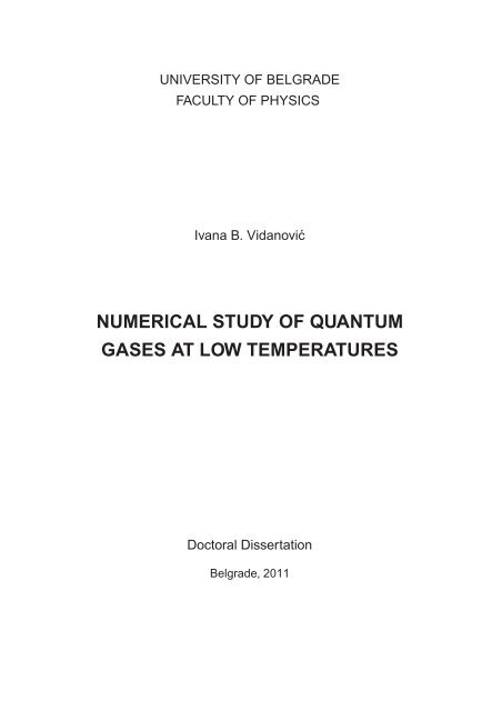
Figure 1.1: The hallmark of the Bose-Einstein condensation - a prominent densitypeak appears below the condensation temperature. Density profiles of the expandedcloud are shown at three different temperatures. From the left to the right we seebosonic cloud right above the condensation transition, just below the condensationtransition and in the regime with almost a pure condensate. The experimental resultis originally presented in Ref. [3] and this figure is taken from Ref. [5].the BEC, the relationn(0)λ 3 T ≈ ζ(3/2) ≈ 2.61238 (1.15)holds. Not surprisingly, this condition is very close to the intuitive argument givenat the beginning of the Chapter.The noticeable feature of the condensate phase in the harmonic trap, not presentin the gas phase, is a prominent density peak located at the trap center that reflectsmacroscopically occupied ground state which has the symmetry of the trap potential,superimposed onto the broad thermal distribution. This is illustrated in Fig. 1.1.A bimodality of the density distribution is an important signature of the onset ofBose-Einstein condensation.An important and convenient aspect of the harmonic trap is that the singleparticleground-state is localized both in the real and in the momentum space.Hence, beside static density profiles of the trapped atoms, another possibility forthe experimental differentiation of the phases is free expansion of the gas from thetrap. Initially, the gas is in the thermal equilibrium in the trap, and then suddenlythe trap is switched off and the gas is allowed to expend freely. To describe thethermal gas we use the semiclassical approximation. The density profile after the7

expansion time t is given by [21]= 1λ 3 Tn th (⃗r, t) = 1(2π) 3 ∫∏σ=x,y,z(d⃗pd⃗r 01e β(H(⃗r 0,⃗p)−µ)− 1 δ3 (⃗r − ⃗r 0 − ⃗p M t )) ( 1/21ζ1 + ωσt 2 2 3/2 e βµ− βM 2„«)ωx 2 x21+ωx 2 + ω2 y y2t2 1+ωy 2 + ω2 z z2t2 1+ωz 2t2 For long expansion times we find an approximate expression for the density distributionof a thermal gas in the form [21]n th (⃗r, t) ∼ 1 ( )βMr2βµ−ζλ 3 3/2 e 2t 2 . (1.16)TAs we see, although the initial density distribution is anisotropic, after the expansionof the thermal cloud, we obtain an isotropic density profile. Another important thingthat we learn from the result (1.16) is that expanded density profiles actually carryinformation on the initial velocity distribution of the cloud. This becomes obviouswhen we rewrite Eq. (1.16) asn th (⃗r, t) ∼ 1 ( )ζλ 3 3/2 e − Mv22k B T. (1.17)TNow we compare this behavior with the expansion of a pure condensate (N = N 0 ) inthe ground state of the trap (1.6). For the time evolution of a quantum mechanicalstate, we have∫ˆ⃗p2−itψ HO (⃗r, t) = 〈⃗r|e 2M |ψHO 〉 =⃗p2−itd⃗p 〈⃗r|⃗p〉e 2M 〈⃗p|ψHO 〉.=1π 3/4∏σ=x,y,z( ) −14(1 + itωσ ) −1 −2 e σ2 Mωσ 1−itωσ2 1+t 2 ωσ 2 . (1.18)Mω σFrom Eq. (1.18) we conclude that in the limit of long propagation times, the condensatewidths are given by (ω σ /M) 2t 1 [19]. Obviously, the expansion of the groundstate is spatially anisotropic and the aspect ratio of the cloud is inverted duringthe expansion. The behavior is substantially different from the isotropic expansionof the thermal cloud and can be used as a diagnostic tool for the presence of thecondensate in the system.Now that we have introduced the theoretical notations, in the next subsection8

we discuss in some detail the experimental realization of a BEC.1.2.2 Experimental realizationAs already mentioned, it was a pursuit of the clear physical realization of a veryfundamental concept of a BEC that triggered an enormous amount of the experimentaleffort starting in the eighties of the last century. Although today BECsof different atoms are readily produced in laboratories worldwide, the creation ofquantum degenerate atomic gases took many years during which many experimentaltechniques at the forefront of technology were developed. In this subsection we givea basic description of today’s typical experimental setup with a very brief historicaloverview. The main reference we rely on is Ref. [21].Already in the early experimental phase of the quest for nanokelvin temperatures,possibility of storing atoms in any type of a vessel was ruled out. Instead, a properconfiguration of magnetic, optical or combined magneto-optical potential is used asan external confining potential, usually called a trap. Atoms are trapped around thepotential minimum due to interaction of their induced magnetic or electric dipolemoments with external field. In most cases, harmonic potentialV (⃗r) = 1 2 M(ω2 xx 2 + ω 2 yy 2 + ω 2 zz 2 ) , (1.19)is a reasonable approximation of the external trap potential. Different trap configurationshave been experimentally realized: for instance, highly elongated traps(which can be considered as effectively one dimensional), or pancake shaped traps(effectively two-dimensional regime). Beside this common type of a harmonic confinement,periodic external potentials (optical lattices) are widely used in nowadaysexperiments. We will mainly consider an axially-symmetric harmonic trap potential,with the radial trap frequency ω x = ω y = ω. The usual form of the potential isV (⃗r) = 1 2 Mω2 (ρ 2 + λ 2 z z2 ) , (1.20)where we introduce the trap aspect ratio λ z = ω z /ω. Typical values of the trapfrequencies are of the order of 2π × (10 − 100)Hz, with a typical length scale of theorder of several microns.The initial attempts to realize a BEC, focused on the spin-polarized hydrogen.The hydrogen was singled out among other atom types since it remains in the9

gas phase even at very low temperatures. Correspondingly, many techniques wereoriginally developed for the hydrogen samples. Yet, it turned out that alkali atoms,such as Rb, Li, Na, K, have several advantages over hydrogen. First, they can becooled using laser cooling techniques [21, 22] by the commercially available laserswhose wavelengths correspond to the transitions between energy levels of alkaliatoms. Second, stronger elastic collisions allow an improved cooling rate in theprocess of evaporative cooling [21, 23]. Evaporative cooling can be performed inseveral ways. Usually it is implemented by lowering the trap depth. In this way,atoms with more than average energy are removed from the trap, hence allowing theremaining atoms to equilibrate at lower temperature. Another way is to performthe radio frequency forced evaporation by transferring internal state of energeticatoms into the untrapped configuration. By varying the used frequency, the finalvalue of the temperature can be controlled. One of the crucial steps that finally ledto the achievement of the high phase-space density necessary for the observation ofa BEC was precisely the combination of the laser cooling and evaporative coolingtechniques.Another vital experimental aspect is the characterization of a BEC once it hasbeen produced. In typical experiments, the sample has the size from 10 3 to 10 6bosonic alkali atoms, trapped in the external field in the space volume of (100µm) 3 ,with a density in the range 10 18 −10 21 m −3 , and the temperature of 100 nK. How thesystem can be probed to confirm that it really represents a BEC and has propertiespredicted theoretically? As usual, the probe has to be “gentle” enough not to perturbthe system significantly, hence cold bosonic gases are mainly probed optically. Thereare several widely used techniques, and we mention the most important ones.From early experiments until today, the absorption imaging remains the mostused tool for characterization of a BEC. The sample is irradiated by a laser beamresonant with an internal atomic transition and the shadow of the sample is measuredby a CCD camera. Such a procedure may not produce the desired resultsalways, since the image can be blacked out by the high density of the sample. Forthis reason, once the BEC regime has been reached, the trap is usually turned off,the cloud is allowed to expand freely for several seconds, and then the absorptionimaging is performed. The procedure is denoted as the time-of-flight (TOF) measurement.In general, the quantity which is measured in this way is the opticaldensity of the sample (responsible for the absorption). It is proportional to thecolumn particle density, which can be determined by this measurement technique.10

In the first papers [3, 4], the TOF approach was used to prove the presence of thecondensate in the sample based on the signatures discussed in subsection 1.2.1 forthe noninteracting gas in the harmonic trap. Time-of-flight images revealed theemergence of density peaks on top of broad thermal distributions. Also, the peak inthe density became more and more prominent as the temperature decreased further.In addition, the measured velocity distribution demonstrated stark contrast in theregimes above and below condensation temperature, being isotropic in the formercase and highly anisotropic in the latter case, reflecting the anisotropy of the trap.From the measured density profiles, other quantities can be also estimated. Usually,noninteracting gas model is used for the extraction of the sample properties. Forexample, the temperature of the sample is determined by fitting a function (1.16)to the experimental data for the thermal cloud.Obviously, the TOF measurements are destructive and make the observation ofthe condensate dynamics quite complicated. With this technique a real-time monitoringof a dynamical process requires many steps: initially, a BEC is produced,then in the certain interval time some dynamical process happens, and finally theBEC is destructively imaged. To obtain another piece of information on the dynamicalevolution, for another value of the time of evolution, the whole procedurehas to be repeated, starting from the production of a BEC. Another difficulty arisesin the interpretation of experimental data. The noninteracting gas model for theharmonic trap is simple enough to enable quantitative explanation, however, theaccurate description of the expanding interacting gas at finite temperature is farmore complicated. Very early [16], dispersive imaging techniques were utilized forgathering in-situ information on the density profiles of cold gases in a nondestructiveway. One of the techniques used successfully for an in-situ imaging of dense samplesis a phase-contrast imaging. This procedure can be implemented through two differentexperimental protocols. In the first one, the light diffracted from the sampleis recorded, while in the second one, the interference patterns of the phase-shiftedincident light and the diffracted signal are measured. In this way, information on thecomplex phase acquired by the non-resonant light in the atomic sample is extracted[24]. Again, the quantity which is measured is the optical density along the line ofsight, yet the measurement can be performed even for a very dense samples. Thistype of measurement allows multiple imaging of the same cloud, hence it is muchmore convenient for studying condensate dynamics.Up to now we have only considered a noninteracting gas of particles, because11

this is the system that was originally used to derive the Bose-Einstein distribution.Of course, realistic systems require many-body approach including interactions andthe noninteracting description is only an approximation. Now we discuss the typeand strength of interactions in the dilute atomic systems, and later in the thesis wewill explain how they modify the noninteracting picture.A predominant interaction in dilute cold atom systems is a two-body interaction,typically in the form of scattering of atoms. In this thesis we consider only a shortrange van der Waals interaction between charge-neutral atoms. A dipole-dipole interactionis also present, but usually can be neglected in the case of alkali atoms.However, it plays prominent role in recent experiments with 52 Cr, where the effectsof long-range dipolar interaction become measurable [25]. Due to diluteness of thesystem, a typical atom-atom distance is larger then the effective interaction range,and details of the short-range interaction potential are not so important. In thelow-energy low-momentum limit, the potential can be parameterized by a single parametera, representing the atomic s-wave scattering length. In the pseudopotentialdescription, the van der Waals interaction is replaced by a contact potentialV int (⃗r − ⃗r ′ ) = gδ(⃗r − ⃗r ′ ) , (1.21)where the interaction strength is given byg = 4π2 aM . (1.22)The interaction is repulsive for g > 0 and attractive in the opposite case. It is knownthat a BEC with attractive interactions is unstable toward collapse if the particledensity is high enough [5]. In this thesis, we confine the discussion to the repulsivelyinteracting BECs.In general, scattering properties of atoms depend on their internal states. Thisfact allows the adjustment of the s-wave scattering length by the control of the externalparameters of the system. More specifically, several atomic species exhibit theso-called Feshbach resonance - dependence of the scattering length on the externalmagnetic field B, which is given by the expressiona(B) = a BG(1 + ∆ BB − B ∞), (1.23)12

where a BG is the off-resonant scattering length, B ∞ is the resonance position and∆ B is the resonance width. Feshbach resonance is a very useful tool that allowsfine and versatile tuning of the interaction strength in the cold atom systems overa range of several orders of magnitude from highly repulsive to highly attractiveregime. A phenomenon is well known in atomic and nuclear physics as Feshbach-Fano resonance [26, 27]. Beside the original reference by Tiesinga et al. [28] whichanalyzed the benefits of using the resonance in the experiments with ultracold atoms,the underlying theory has been discussed in the review paper by Chin et al. [6] andin several textbooks [19, 29]. Here we give only a brief explanation, based on a factthat two atoms can interact via an energetically open or closed channel. These twochannels are coupled and include Zeeman terms. By tuning the external magneticfield it is possible to make a bound state of a closed channel resonant with theincome energy in the open channel. In that case the scattering length diverges, asgiven in Eq. (1.23) for B = B ∞ . The properties of Feshbach resonances are exploitedin many experiments and one of the topics in this thesis will explore some relatedrecent experimental results.To summarize the subsection, the achievement of the BEC regime took a lot ofeffort and many techniques had to be developed for this purpose. However, once thishas been achieved, the cold atomic systems have become the cleanest experimentalsetting for studying macroscopic quantum phenomena. All parameters of thesesystems are highly controllable and tunable: the geometry, temperature, densityand even the type and the strength of interaction. For this reason the field of ultracoldatoms is still in the process of strong expansion and cross-collaboration withother fields, and further new important insights are expected.1.2.3 Interacting bosons at low temperaturesAfter discussing physical characteristics of cold bosonic atoms, we are ready to writedown the Hamiltonian of the system:∫Ĥ =d⃗r(− ˆψ † (⃗r) 22M ∇2 ˆψ(⃗r) + V (⃗r) ˆψ† (⃗r) ˆψ(⃗r) + g )2 ˆψ † (⃗r) ˆψ † (⃗r) ˆψ(⃗r) ˆψ(⃗r) . (1.24)Here ˆψ † (⃗r) and ˆψ(⃗r) are bosonic field operators in the second quantized form, andsatisfy commutation relations [ ˆψ(⃗r), ˆψ(⃗r ′ )] = 0, [ ˆψ † (⃗r), ˆψ † (⃗r ′ )] = 0, [ ˆψ † (⃗r), ˆψ(⃗r ′ )] =δ(⃗r−⃗r ′ ). On the right hand side of Eq. (1.24) we have the kinetic energy term, poten-13

tial energy of particles in the external trap given by V (⃗r) and interaction term whichstems from ∫ d⃗rd⃗r ′ V int (⃗r − ⃗r ′ ) ˆψ † (⃗r) ˆψ(⃗r) ˆψ † (⃗r ′ ) ˆψ(⃗r ′ ) = g ∫ d⃗r ˆψ † (⃗r) ˆψ † (⃗r) ˆψ(⃗r) ˆψ(⃗r).Hamiltonian given by Eq. (1.24) without the external trap potential was studiedin the early work of Bogoliubov in relation to superfluidity observed in 4 He [30].It represents the starting point in theoretical studies of a BEC. Here we give anelementary exposition of main ideas of the Bogoliubov and, in parallel, we introduceconcepts important for the description of an interacting BEC.In the homogenous case, a good quantum number of the system is the wavevector⃗ k. Therefore, we use the decompositionˆψ(⃗r) = 1v 1/2 ∑⃗ ke i⃗ k⃗râ⃗k , (1.25)where â ⃗k are annihilation operators in the occupation number basis, with singleparticleeigenfunctions in the form of plane waves. In the noninteracting limit, weexpect macroscopic occupation N 0 of the ground state that we designate as |N 0 〉. Ifwe take into account the exact relationsâ 0 |N 0 >= √ N 0 |N 0 − 1 >, â † 0|N 0 >= √ N 0 + 1|N 0 + 1 > , (1.26)and the fact that N 0 + 1 ≈ N 0 − 1 ≈ N 0 , we arrive at the following approximationswhich replace operators â 0 and a † 0 with c-numbers: â 0 ≈ √ N 0 and â † 0 ≈ √ N 0 . Theerror made by using this approximation is of the order of [a 0 , a † 0] = 1, and can beneglected compared to the macroscopic value of N 0 . Said another way, we haveapproximated the expression (1.25) byˆψ(⃗r) ≈ ψ + δ ˆψ(⃗r) , (1.27)where ψ = (N 0 /v) 1/2 = n 1/20 is a classical field, and the operator δ ˆψ(⃗r) correspondsto quantum fluctuations around the classical value. The next step in the Bogoliubovapproach is to consider quantum fluctuations as being small and to keep only termsup to the second order in δ ˆψ. With these simplifications we can find an appropriatetransformation which converts the quadratic approximation of the Hamiltonian intothe diagonal form. The final result is the Bogoliubov excitation spectrum of the14

system given by( ) ǫ Bog ⃗k = √ 2⃗ k 22M( 2⃗ k 22M + 2gn 0). (1.28)In the limit of large | ⃗ k|, the spectrum yields excitations of a noninteracting gas. Collectivephenomena appear in the long wavelength limit where the collective phononmode is found [30]. The microscopic derivation of the excitation spectrum (1.28)fits well with the Landau’s phenomenological description of the superfluid. Anotherrelevant quantity that can be derived within the Bogoliubov framework is thecondensate depletion due to interactions at T = 0. The number of non-condensedparticles is proportional to √ na 3 , which for the case of strongly interacting systemsuch as liquid 4 He yields the depletion as high as 90%. For this reason, the superfluidityof 4 He is considered only as an indirect manifestation of the Bose-Einsteincondensation.In general, the relation between the condensation and superfluidity is a subtleone. It can be shown that the macroscopic occupation of the ground state (1.27)introduces the off-diagonal long range order (ODLRO) into the system [31]:lim 〈 ˆψ † (⃗r) ˆψ(⃗r ′ )〉 = n 0 . (1.29)|⃗r−⃗r ′ |→∞However, long range correlations that are the manifestation of a superfluidity may bepresent even without the condensation, as for instance in two-dimensional systems[7].In order to put the phenomenon of Bose-Einstein condensation into a broadercontext, we emphasize that the decomposition (1.27) represents the spontaneousbreaking of the U(1) symmetry related to the conservation of the number of particlesin the system described by the Hamiltonian (1.24). Hence, ψ is the order parameterthat acquires nonzero value in the condensed phase [31, 32].Quantitative tests of the theoretical concepts introduced in this subsection becamepossible only with the experimental realization of Bose-Einstein condensationin dilute vapors of alkali atoms. However, the experiments introduced an importantadditional feature - the inhomogeneity of the system due to the trapping potential.The first theoretical study of a interacting bosonic system in a harmonic trap waspresented in Ref. [33] in relation to the early experiments that were trying to producehydrogen BEC. Since then, different approaches have been used to describe the15

condensation of interacting bosonic gas in an external trap potential. In this thesiswe will work in the mean-field framework, with an order parameter introduced in asimilar manner as in Eq. (1.27). The exposition of the mean-field framework for thetrapped system is given in Chapter 4.Throughout the years, a lot has been learned about the phenomenon of a BEC bya powerful combination of ingenious experiments and equally ingenious theoreticalmodeling. Yet, despite the intensive progress in the field, there are still many openquestions related to the fundamental topics, as will be indicated throughout thethesis.1.3 This thesisThe main objective of this thesis is a thorough analysis and understanding of twointeresting physical scenarios for the manipulation of cold bosonic atoms that haverecently came into the focus of the experimental research. Namely, we will firstexplore the details of the phase diagram of a rotating ideal bosonic gas in an anharmonictrap. As a second topic, we will investigate the nonlinear features of theexcitation of collective oscillation modes by a modulation of the interaction strength.On the way to accomplish this, in Chapter 2 we work out the details of thenumerical method which is capable of providing us with a highly-accurate energyspectrum of a few-body system. As we already saw in the subsection 1.2.1, the accurateinformation on the energy spectrum of the system is required for the descriptionof a BEC phase transition. The method that we elaborate on is based on the exactdiagonalization of the short-time evolution operator and was introduced earlier in asimplified form [9]. To understand the benefits of the method, we first analyze theerrors associated with space discretization of the time-evolution operator. Basedon analytical and numerical analysis, we show that the discretization error vanishesexponentially with 1/∆ 2 , where ∆ is the discretization spacing. This nonperturbativebehavior highly outperforms polynomial errors in discretization spacing ∆which arises in the common real-space discretization of the Hamiltonian. The keycomplexity of the method is the accurate calculation of the matrix elements whichare given by transition amplitudes. To address this requirement, we apply recentlyintroduced effective action approach [10, 11] for obtaining short-time expansion ofthe propagator to very high orders. We demonstrate high efficiency of the methodon several one- and two-dimensional models.16

Having the efficient numerical method at our disposal, in Chapter 3 we studyproperties of a rotating ideal gas. The introduction of the angular momentum intothe system is one way of reaching the highly correlated regime in the cold atomsetup. As will be explained, beside other effects, a rotation effectively introduces adeconfining component into the trap potential. Particularly, in the regime of a fastrotation, the gas may experience the complete deconfinement. Hence an additionalquartic potential was used for the trapping in the experiments from Ref. [12], butthe interesting regime of fast rotation has not been completely understood. Usingthe exact diagonalization of a time evolution operator, we study numerically Bose-Einstein condensation in the modified external potential which is a combination ofthe harmonic and quartic component. The shape of the potential changes fromconvex with a single minimum to the Mexican hat shape, depending on the rotationfrequency. We explore how the change of the trapping potential influences the phasediagram properties. We also calculate the density profiles of the gas and time-offlightpictures in different regimes and find that typical time-scales for free expansionare increased by an order of magnitude in the delicate regime of fast rotation.In Chapter 4, we continue and expand a brief exposition of subsection 1.2.3, anddiscuss several different mean-field frameworks for the description of properties of aweakly interacting BECs. First we present the zero temperature mean-field description.We neglect quantum fluctuations and assume that all atoms are condensed atT = 0. In that case, we show that BEC properties are captured by the effectivenonlinear equation, the famous Gross-Pitaevskii equation [34, 19, 13, 14]. Then wemove to the study of finite-temperature mean-field models of BEC. The relevanceof this aspect is two-fold: on one hand, mean-field models are widely used for theinterpretation of experimental data, and on the other hand, from the conceptualpoint of view, it turns out that different models suffer from different unphysicaldrawbacks. We review and compare the existing models by calculating density profileswithin different approximations. To illustrate the influence of weak interactionson the Bose-Einstein condensation, we re-derive the mean-field interaction-inducedshift of the condensation temperature.Chapter 5 deals with the collective excitations of BEC in the nonlinear regime.Characteristics of a BEC can be probed by monitoring its dynamical response tothe external perturbation. Usually, the ground-state BEC is produced and thenit is perturbed by a modulation of the external trap potential. A specific featureof the recent experiment [15] is the harmonic modulation of the s-wave scattering17

length via a Feshbach resonance, yielding a time-dependent interaction strengthg = g(t). An external driving frequency Ω is used for the modulation, and dependingon its closeness to some of the condensate eigenfrequencies, either a resonant ornon-resonant behavior can be observed. This is a new venue for studying nonlineardynamical regime, since the equation governing the condensate dynamics on themean-field level is nonlinear, and large amplitude oscillations are readily producedin the resonant regime. By combining different analytical and numerical methods weanalyze how nonlinear effects influence the properties of the excited collective modes,with implications on the interpretation of the actual experimental data. Prominentnonlinear features, such as: mode coupling, higher harmonics generation, and significantshifts in the frequencies of collective modes are found and quantitativelyexplained using an analytic perturbative approach.At the end of each chapter, we present possible future directions for extending thestudy of research topics of this thesis. Finally, we summarize all results in Chapter6. Additional material and derivations are organized in Appendices.18

Chapter 2Properties of quantum systems viadiagonalization of transition amplitudesDeep in the condensate phase, features of cold atoms are determined by low-lyingenergy levels: ground state and few excited states corresponding to the thermalcloud. On the other hand, thermodynamic properties and details of the BEC phasetransition are determined by the full energy spectrum. As we have seen in Chapter1, the exact calculation of the condensation temperature, even for an ideal bosonicgas, requires a summation over the whole energy spectrum of the system. Dueto its simplicity, the semiclassical approximation is widely used for this purpose.In this Chapter we work out details of a numerical method based on the exactdiagonalization of a time-evolution operator that allows us access to a very largenumber of numerically exact energy levels of few-body systems. Afterwards, inChapter 3, we use the method to find the condensation temperature of the fastrotatingideal gas in an anharmonic trap.In the standard operator formulation of quantum mechanics, the description ofa physical system is based on constructing the Hamilton operator Ĥ. Properties ofquantum systems are then obtained by solving the corresponding time-independentSchrödinger equation,Ĥ|ψ〉 = E|ψ〉 . (2.1)Exact solutions can be found only for a very limited set of simple models. A widevariety of analytical approximation techniques has been developed in the past fortreatment of such problems. In addition, the last two decades have seen a rapidgrowth in the application of different numerical methods for solving the Schrödingerequation. Approaches based on real-space discretization start from some given finitedifferenceprescription. Such methods have been extensively studied in the past, andthe main difficulties follow from the finite-difference representations of the kineticoperator.A numerical approach based on diagonalizing of the evolution operator, intro-19

2. Diagonalization of Transition Amplitudesduced in Ref. [9], does not suffer from problems with the representation of differentialoperators on real-space grids, and has substantial advantages in practical applicationsto few-body problems. Effectively, in this way the problem is transferred fromthat of representing the kinetic operator on a real-space grid to the calculating ofcorresponding transition amplitudes. Detailed analysis of the errors associated withthe implementation of this approach is the main objective of this Chapter. It providesfull understanding of the method and allows its optimal use, as well as furthersignificant improvements within a generalized calculation scheme.The advantages of the method discussed here [9, 35, 36, 37] follow from two keyproperties. First, the objects being diagonalized are transition amplitudes, which arewell defined irrespective of discretization scheme, i.e. the exponential of the Hamiltonianeffectively regularizes the kinetic operator, making possible representations ofthe evolution operator that do not depend on the space grid. Second, the successfuldiagonalization of the evolution operator exp(−tĤ) for any time of propagation timmediately gives the solution of the eigenproblem for the Hamiltonian. Thus, thetime of propagation in this approach is just an auxiliary parameter. Said anotherway, we use the time-dependent evolution operator to extract time-independentinformation regarding the quantum system. If one could calculate transition amplitudesexactly, then the obtained results for the energy eigenproblem would notdepend on the time of propagation. However, in practical applications one uses someapproximation scheme to calculate the amplitudes, and in this case the precision ofthe obtained results for energy eigenvalues and eigenstates does depend on time t.The general applicability of the outlined method follows from the fact that one canuse short-time propagation amplitudes to obtain highly accurate results.In order to complete this numerical method and make it generally applicable, itis necessary to address the following key questions:1. How to analytically estimate the effects of spatial discretization?2. How to optimize the choice of evolution time t, so as to minimize errors?3. How to accurately calculate transition amplitudes?The authors in Ref. [9] have only briefly commented on the first two questions,and numerically determined the values of parameters that can be used for precisecalculations of energy eigenvalues and eigenstates for several models. In this Chapterwe address the above questions, which have not been fully answered before. First we20

2. Diagonalization of Transition Amplitudespresent the method and notation, and identify the sources of the errors present inreal-space discretization approaches. Then we analyze in detail the above questions1 and 2, and discuss the effects of discretization on the numerically calculated valuesof the observables for a given physical system. We analytically derive estimates forerrors stemming from space discretization coarseness, finite size effects, and choice ofthe evolution time parameter t. All the analytically derived results are numericallyverified to hold on several instructive models.Errors associated with the time of evolution parameter t (question 3 above) mustbe carefully taken into account and may substantially limit the precision of numericalcalculation in the diagonalization method. This problem was not addressed atall in Ref. [9], but has been addressed recently [38, 39, 40, 41, 42] using various approaches.We significantly improve the method by applying the recently introducedeffective action approach [43, 44, 10, 45, 46, 11] to completely resolve the problemformulated in question 3. We stress that use of higher-order effective actionsrepresents an efficient and numerically inexpensive way to calculate transition amplitudes,and leads to many orders of magnitude increase in precision of calculatedproperties of the system. We will demonstrate on several lower-dimensional modelshow use of higher-order effective actions significantly reduces numerical errors andsystematically improves the obtained energy eigenvalues and eigenstates.This Chapter gives a complete analysis of the method based on the diagonalizationof transition amplitudes, providing us with necessary analytical knowledge toestimate errors of all types associated with this method and to numerically very accuratelycalculate large numbers of energy eigenvalues and eigenstates. This invitesvarious applications of the method to the study of few-body quantum systems, someof which are discussed throughout the thesis.The expressions written throughout the second and third section are, for compactnessof notation, for one particle in one dimension. Extension to more particlesand dimensions is straightforward, just as with the above short-time transitionamplitude. Note that we are working in imaginary time, which is well suited fornumerical calculations and does not affect in any way calculated energy levels norother time-independent properties of the system. We have also set to unity in thisChapter.21

2. Diagonalization of Transition Amplitudes2.1 Space-discretized Schrödinger equationIn the coordinate representation the time-independent Schrödinger’s equation takesthe form∫dy 〈x|Ĥ|y〉 〈y|ψ〉 = E 〈x|ψ〉 . (2.2)The standard way to numerically implement exact diagonalization is to go fromcontinuous coordinates x to ones living on a discrete space grid x n = n∆, where∆ is a given spacing and n ∈ Z. Integrations in the above equation are performedusing the simple rectangular quadrature rule, or some higher-order finite-differenceformula. This completes the transition to the space-discretized counterpart of thecontinuous theory, however, to represent this on a computer we still have to restrictthe integers n to a finite range. This is equivalent to introducing a space cutoff L, orputting the system in a infinitely high potential box. For example, the rectangularquadrature rule leads to the following space-discretized Schrödinger equationN∑cut−1m=−N cutH nm 〈m∆|ψ〉 = E(∆, L) 〈n∆|ψ〉 , (2.3)where H nm = ∆ · 〈n∆|Ĥ|m∆〉, N cut = [L/∆], and square brackets represent theinteger part of the argument. As a result, we have obtained a 2N cut × 2N cut matrixthat represents the Hamiltonian of the system. The eigenvalues of this matrix dependon the two parameters introduced in the above discretization process: cutoffL and discretization step ∆. Continuous physical quantities are recovered in thelimit L → ∞ and ∆ → 0. The outlined procedure is very useful in dealing withspatially localized physical problems, such as electronic structure calculations insemiconductor and polymer physics [47].The two approximations involved in the discretization procedure, characterizedby parameters ∆ and L, are common steps in solving eigenproblems of Hamiltoniansin e.g. electronic structure calculations [47], and as such have been extensivelyanalyzed. The imposed constraint on the values of spatial coordinates to the finiteinterval (−L, L) is a valid approach for capturing information on localized eigenstates.In this approximation the system is effectively surrounded by an infinitelyhigh wall, and as the cutoff L tends to infinity, we approach the exact energy levelsalways from above, which is a typical variational behavior. Therefore, we designateerrors associated with the cutoff L as variational. The effects of the discretization22

2. Diagonalization of Transition Amplitudesstep ∆ are more complex, and follow from the fact that the kinetic energy operatorcannot be exactly represented on finite real-space grids. For example, a typicalnaive discretization of the kinetic energy operator gives in our notation the followingHamiltonian matrix elements [48]⎧⎪⎨ 1/∆ 2 + V (n∆) if n = mH nm = −1/(2∆⎪⎩2 ) if |n − m| = 10 otherwise.(2.4)Note that in the absence of a potential term V in the Hamiltonian, the above definitioncorresponds to a tight-binding model [48]. This prescription leads to numericalresults for eigenvalues which in the ∆ → 0 limit converge to the exact continuumvalues as ∆ 2 . The errors associated with this approach have non-variational behavior,i.e. the obtained results are not always upper bounds of the exact energy levels.Several papers discuss this issue and analyze the behavior of errors in the direct diagonalizationapproach (for more details, see Refs. [49, 50] and references therein).The state-of-the-art in this approach is a set of systematically improved prescriptionsfor discretization of the kinetic energy operator, which speeds up convergenceto the continuum limit to higher powers of ∆ 2 . However, within this approach convergenceis always polynomial in ∆. Some recent results [51] also exist on extensionsof this approach that provide effective variational behavior of the discretized kineticenergy operator.As outlined in the Introduction, we focus on an alternative approach, based onsolving the eigenproblem of the corresponding transition amplitudes as proposed in[9]. The central equation isor in the discretized formN∑cut−1e −tĤ|ψ〉 = e −tE |ψ〉 , (2.5)m=−N cutA nm (t) 〈m∆|ψ〉 = e −t E(∆,L,t) 〈n∆|ψ〉 , (2.6)where A nm (t) = ∆·A(n∆, m∆; t) = ∆·〈n∆|e −tĤ|m∆〉. In this approach the time ofevolution t plays the role of an auxiliary parameter. This parameter is not relatedto the discretization, and in a continuous theory it does not affect the obtainedeigenvalues and eigenstates. However, in a discretized theory the numerically calcu-23

2. Diagonalization of Transition AmplitudesA0.30.20.10-4-3-2-1-10-212-3x 34 -40123y4Figure 2.1: Harmonic oscillator transition amplitude as a function of coordinates xand y for t = 1.lated eigenvalues and eigenstates will necessarily depend on this parameter as well,as emphasized by the right-hand size of Eq. (2.6). Therefore, the original problemis now transformed into the eigenproblem of the matrix A nm (t), whose indices takeall integer values in the range −N cut ≤ n, m < N cut , where N cut = [L/∆].Fig. 2.1 shows how a typical transition amplitude, in this case that of a harmonicoscillator, depends on coordinates x and y. The transition amplitude of a harmonicoscillator with the Hamiltonian ĤHO = ˆp 2 /2 + ˆx 2 /2 can be calculated analyticallyand is given by explicit the expression:A HO (x, y; t) =√ [ 12π sinh t exp − 1 ((x 2 + y 2 ) cosht − 2xy )] . (2.7)2 sinh tNote that the consideration is general since non-trivial mass and frequency of theharmonic oscillator can be easily taken into account by a simple rescaling of thecoordinate and momentum. As can be seen from the figure, transition amplitudesare spatially well localized. This is particularly simple to understand for the shorttimes of propagation that we consider for a general case in the external potential.For a very short propagation times, transition amplitudes can be roughly calculatedas:A(x, y; t) ≈ √ 1 e −(x−y)2 −tV ( x+y2t 2 ) . (2.8)2πtFrom the last expression, we see that the kinetic term exponentially localizes thetransition amplitude matrix to the vicinity of the main diagonal. Similarly, the24

2. Diagonalization of Transition Amplitudespotential brings about exponential localization along the main diagonal around itsminimum. The localization of dominant values of the transition amplitude to asmall area in the x − y plane gives practical justification for introduction of spacecutoff L in this approach.80706050t = 0.125t = 0.040t = 0.020t = 0.015E k403020100-100 5 10 15 20 25 30 35 40 45kFigure 2.2: Eigenspectrum of a free particle in a box. Eigenvalues E k are given asa function of level number k. The solid line gives the exact parabolic dispersionE k = π 2 (k + 1) 2 /8L 2 , while the dashed line presents results calculated in the tightbindingapproximation. The graph also shows numerical results obtained by thediagonalization of transition amplitudes for different values of time of evolution t.All the numerical calculations are for L = 6 and ∆ = 0.25, hence N cut = L/∆ = 24.In the continuum theory, the transition amplitude eigenproblem is mathematicallyequivalent to the Schrödinger equation. It is important to stress, however,that the procedure of space discretization introduces important differences betweeneigenproblems (2.3) and (2.6). In particular, as we will show in the next section, theprocedure based on the diagonalization of transition amplitudes leads to much faster(non-polynomial) convergence. An illustration of the relation of these two calculationschemes is shown in Fig. 2.2 which compares the exact parabolic dispersion ofa free particle in a box with numerical calculations based on diagonalizations of theHamiltonian and of the transition amplitudes. From the figure we see that the timeparameter t in the transition amplitude approach plays an important role. Increaseof the evolution time t gives better agreement with the exact dispersion relation.25

2. Diagonalization of Transition Amplitudes2.2 Discretization effectsThe free-particle transition amplitudeA free (x, y; t) = 1 √2πte −(x−y)2 2t (2.9)satisfies the relation∫dxA free (x, y; t) = 1 . (2.10)The consequence of this is conservation of probability. In the space-discretizedanalogue of this model x = n∆, y = m∆, and the transition amplitude is A freenm (t) =∆ A free (n∆, m∆; t). Using the Poisson summation formula√∑ πe −αn2 =αn∈Z∑n∈Ze − π2α n2 , (2.11)we find that the space discretized free particle amplitude satisfies∑n∈ZA freenm(t) = ∑ e −2π2 ∆ 2 n2t ≈ 1 + 2e −2π2 ∆ 2 t . (2.12)n∈ZConservation of probability is thus obtained only in the continuum limit ∆ → 0.Note that the effect of discretization is non-perturbative in discretization step ∆,i.e. it is smaller than any power of ∆. The effect of discretization is also universalin that it holds for all models, since the free particle transition amplitude is thedominant term in the short time expansion of the transition amplitude of a generaltheory.To show this explicitly we use the short time expansion of the transition amplitudeof a general theory [44] to show that∫dxA(x, y; t) = 1 √2πt∫dxe − 1 2t x2 ∑ lt l f l (x, y) , (2.13)where f 0 = 1 and the other functions f l are determined by the potential and itsderivatives. Writing the even part of f l (x, y) as g(x 2 , y) we find∫dxA(x, y; t) = √ 1 ∑t l g l (2t 2 ∂ t , y) √ t . (2.14)tl26

2. Diagonalization of Transition AmplitudesSimilarly, using the above Poisson summation formula, we find∑∫A nm (t) −n∈ZdxA(x, y; t) = 2 √t∑lt l g l (2t 2 ∂ t , y) √ te −2π2 ∆ 2 t . (2.15)Performing the indicated differentiations the right hand side becomes exp(− 2π2∆ 2 t) ·∑l h l(y)t l . One could now calculate the functions h l from the short time expansionsof f l . The p-level effective action gives a short time expansion, which is truncatedat order t p . As a result, ∑ l h l(y)t l is a polynomial in time of order p. The dominantshort time behavior is thus given by the universal exponential term. As a consequence,the transition of a general model to its space discretized form is given by∑∫A nm (t) −n∈ZdxA(x, y; t) ∼ e −2π2 ∆ 2 t . (2.16)This universal and non-perturbatively small deviation from the continuum indicatesthat one should center numerical calculation schemes on transition amplitudesrather than the Hamiltonian. By diagonalizing the transition amplitude for anytime of propagation t we obtain the energy eigenvalues and eigenfunctions∫dy A(x, y; t)ψ k (y) = e −tE kψ k (x) . (2.17)To solve this numerically we first discretize space with discretization step ∆, andsecond we introduce a spatial cut-off L such that |x| < L. Amplitudes are now2N cut × 2N cut matrices whose diagonalization leads to 2N cut eigenstates ψ k andeigenvalues e −tEk(∆,L,t) .As we have seen, discretization introduces a non-perturbatively small error intransition amplitudes proportional to exp (−2π 2 t/∆ 2 ). We should therefore expectthe discretization error for energy eigenvalues to beE k (∆, L, t) − E k ∼ − 1 t e−2π2 ∆ 2 t . (2.18)We have numerically investigated this for a diverse set of models and have shown theabove relation to hold in all cases. It is also illustrative to verify this for analyticallytractable models. Using the known analytical expressions for transition amplitudeand energy eigenstates for a free particle in a box [52, 53], as well as the Poissonsummation formula in Eq. (2.11), we find that the energy eigenstates of the space27

2. Diagonalization of Transition Amplitudesdiscretized model satisfyE k (∆, L, t) − E k = − 2 t e−2π2 ∆ 2 t cosh π2 (k + 1)tL∆, (2.19)| E 0 (∆, L, t) - E 0 |10 -20 110 -4010 -6010 -8010 -100Ht = 0.25t = 0.5t = 110 -310 -410 -510 -60.2 0.4 0.6 0.8 10.2 0.3 0.4 0.5 0.6 0.7 0.8 0.9 1∆10 20 0 0.2 0.4 0.6 0.8 1| E k (∆, L, t) - E k |10 -20 110 -4010 -6010 -8010 -10010 -120∆ E 0∆ E 14∆ E 24∆ E 34∆ E 44∆ E 54Figure 2.3: Top: Plot of |E 0 (∆, L, t)−E 0 | for a free particle in a box as a function of∆ for different values of time of evolution t and L = 6. For comparison, we also plotthe corresponding deviations of numerical results (designated by H) obtained usingdirect diagonalization of the space-discretized Hamiltonian, defined by Eq. (2.4).Bottom: This plot shows how the deviations |E k (∆, L, t) − E k | depend on t forseveral energy levels k. The parameters used are L = 6, ∆ = 0.2. In both plots thedashed lines represent discretization error estimates given in Eq. (2.19).t28

2. Diagonalization of Transition Amplitudes12010080t = 0.015t = 0.020t = 0.040t = 0.125E k60402000 10 20 30 40 50 60 70 80 90kFigure 2.4: Harmonic oscillator dispersion relation. The solid line gives the exactlinear dispersion E k = k +1/2. The points correspond to numerically calculated energyeigenvalues E k as function of level k. We show the results of the diagonalizationof transition amplitudes for several values of t. In this plot L = 12, ∆ = 0.25.where E k = π2 (k+1) 2and k = 0, 1, 2, . . . As expected, the universal term gives the8L 2dominant ∆ dependence. One obtains similar analytical results for the case of theharmonic oscillator.The non-perturbatively small effect of spatial discretization is the reason whythe new method highly outperforms direct diagonalization of the Hamiltonian andleads to much smaller errors for the same size of discretization step ∆. In additionto this the free parameter associated with the method, the time of evolution t, canbe used to further minimize errors. As illustrated in Fig. 2.2, while keeping ∆ fixed,we can adjust time t to obtain much smaller errors and practically reproduce theexact spectrum of the theory. This is also evident in Fig. 2.3, where we see thatby adjusting t, errors can be reduced by orders of magnitude for fixed value ofdiscretization step ∆.We next consider a harmonic oscillator. Fig 2.4 shows how the presented methodmay be used to obtain energy eigenvalues to high levels. The numerical calculationsagree well with the well known linear dispersion of the harmonic oscillator.Figs. 2.5(top) and 2.5(bottom) display respectively the ∆ and t dependence of thedeviations |E k (∆, L, t) − E k |, showing agreement with the analytically derived estimateof the discretization error given in Eq. (2.18). In order to achieve such a29

2. Diagonalization of Transition Amplitudes| E 0 (∆, L, t) - E 0 |110 -2010 -40Ht = 0.005t = 0.01t = 0.02t = 0.03t = 0.0410 -1 0 0.2 0.4 0.6 0.8 110 -310 -60 10 -50.05 0.1 0.15 0.2 0.25 0.310 -10 1∆| E k (∆, L, t) - E k |10 -2010 -3010 -4010 -5010 -6010 -70∆ E 0∆ E 14∆ E 24∆ E 34∆ E 44∆ E 540.01 0.02 0.03 0.04 0.05 0.06 0.07 0.08 0.09tFigure 2.5: Top: Plot of |E 0 (∆, L, t) − E 0 | for a harmonic oscillator as a function ofdiscretization step ∆ for different values of time of evolution t with L = 12. For acomparison, we also plot the corresponding results (designated by H) obtained usingdirect diagonalization of the space-discretized harmonic oscillator Hamiltonian.Bottom: Plot of the deviations |E k (∆, L, t) − E k | given as a function of time t forseveral levels k. The parameters used are L = 12, ∆ = 0.1. In both plots the dashedlines correspond to the discretization error estimate for E 0 given in Eq. (2.19).high accuracy of numerical results as presented on all graphs, we have used theMATHEMATICA software package [54].Fig. 2.5(bottom) shows how the deviations |E k (∆, L, t) − E k | depend on t forseveral levels k. The plot corresponds to the harmonic oscillator but is typical30

2. Diagonalization of Transition Amplitudesof a general theory. The saturation of errors for large t comes about when thediscretization error, given by the universal estimate in Eq. (2.18), becomes smallerthan the error due to space cutoff L. Analytical estimates for cutoff error are givenat the end of this section. At this point we just mention that the finite size effectscan already be seen in Fig. 2.4, where for high values of level number k numericalresults start to move away from the linear dispersion characteristic of a harmonicoscillator to the parabolic dispersion characteristic of a box potential.We end the section by looking at finite size effects, i.e. errors related to introductionof space cutoff L. For any theory with non-trivial potential, the cutoff Lis artificially introduced and it affects the obtained energy eigenvalues, as we havealready discussed. To estimate the effects of the cutoff, we first note that they areclosely related to the spatial extent of the potential V , as well as the spatial extentof eigenfunctions of the system: errors in the corresponding energy eigenvalues canbe considered small only if the eigenstates ψ k (x) are well localized in the interval|x| < L.The effects of space cutoffs have been previously studied for continuous-spacetheories [55, 56]. The shift in energy level E k (L) −E k is found to be positive in thiscase, and approximately given by the formula(∫ L) −1dxE k (L) − E k = C k (a), (2.20)a |ψ k (x)| 2where a is an appropriately chosen value of coordinate x such that it is larger thanand well away from the largest zero of ψ k (x) but smaller than and well away from thespace cutoff L. The constant C k (a) depends on the normalization of eigenfunctionand the choice of parameter a. For example, the ground state has no zeros, and wecan always choose the value a = 0. In that case, constant C 0 (0) is given by(∫ L) −1C 0 (0) = dx |ψ 0 (x)| 2 , (2.21)−Lwhere we assume that the eigenfunction ψ 0 (x) is normalized, ∫ ∞−∞ dx |ψ 0(x)| 2 = 1.In practical applications, when we use diagonalization of the discretized transitionamplitudes, the errors in energy level will necessarily also depend on theparameter t and other discretization parameters. Here we give a simple estimateof ground energy errors that follows from the spectral decomposition of diagonal31

2. Diagonalization of Transition Amplitudes10 10 110 -10 5 6 7 8 9 10 11 12E k (∆, L, t) - E k10 -2010 -3010 -4010 -5010 -6010 -70∆ E 0 , t = 0.1∆ E 0 , t = 10∆ E 14 , t = 0.1∆ E 14 , t = 10Figure 2.6: Deviations E k (∆, L, t) − E k for a harmonic oscillator as a function ofspace cutoff L for different values of time of evolution t. The discretization step is∆ = 0.1. Solid thin lines give the dominant behavior of Eq. (2.23). The dashedthick lines correspond to the error estimate in Eq. (2.20).Lamplitudes. For large t we have A(x, x; t) ≈ |ψ 0 (x)| 2 e −E0t . Integrating this we findan approximate result for the ground energy of a system with cutoff LE 0 (L, t) ≈ − 1 ∫ Lt ln dxA(x, x; t) , (2.22)In the L → ∞ limit we recover the exact ground energy, so that a simple estimateof finite size effects on E 0 is given byE 0 (L, t) − E 0 ≈ 1 ∫dx |ψ 0 (x)| 2 . (2.23)t−L|x|>LAlthough the above equation is just a rough estimate of the errors introduced by aspace cutoff L, Fig. 2.6 shows that it is in good agreement with numerical resultsfor the harmonic oscillator. In order to clearly demonstrate L-dependence of errorsin this graph, we have used small value of the discretization step ∆, such thatdiscretization errors can be neglected. The dashed lines in the figure represent errorestimates given by Eq. (2.20).Using the data from Fig. 2.6 we can now fully explain the saturation of errorsobserved in Fig. 2.5(bottom). The value of the cutoff L used to obtain this data32

2. Diagonalization of Transition Amplitudeswas L = 12. As can be seen from Fig. 2.6, this value of the cutoff parameter yieldsan error of the order 10 −65 for the ground-state energy for t ∼ 0.1, and of the order10 −40 for energy eigenlevel E 14 . These values exactly correspond to the saturatederrors in Fig. 2.5(bottom).Although in the general case the eigenstates that come into Eqs. (2.20) and(2.23) are not known, we can still use them in conjunction with other approximationtechniques to estimate finite size effects. We also see that, due to the largerspatial extent of higher energy eigenstates, the cutoff-related errors are minimal forthe ground energy. Note however that one is not really interested in the precisecalculation of finite size errors, but only needs to estimate the minimal size of thecutoff L for which finite size effects are negligible. For that purpose one can useeither of the above approximate formulas.2.3 Effective actionsSo far we have considered only integrable models, i.e. models for which we know theexact transition amplitudes. As a result we have thus far encountered and analyzedonly two sources of errors: those associated with discretization step ∆ and cutoffL. The vast majority of models are not integrable. The outlined method is stillapplicable if one uses some approximation for calculating transition amplitudes.As we can see, the precise calculation of transition amplitudes is essential forpractical applications of this method. In Ref. [9] all calculations are based on thenaive approximation for transition amplitudesA (1) (x, y; t) ≈1V (x)+V (y)−t√(2πt)d e−(x−y)2 2t 2 , (2.24)which is correct only to order O(t), and is for this reason designated by A (1) . If oneuses the naive approximation for transition amplitudes, then times of propagationmust be very short for errors to be small enough. Practically, even for short times ofpropagation, such errors are always much larger than the errors due to discretization,and therefore significantly limit the applicability of the method. In addition tothis, the results obtained in the previous section on exactly solvable models suggestthat longer times of propagation generally give smaller errors in the diagonalizationapproach. The trade-off between these effects and its implications on numericalresults have been documented in [9].33

2. Diagonalization of Transition AmplitudesTo address this, in principle one can use Monte Carlo simulations [57, 58] tocalculate amplitudes A to high precision. Although this can effectively resolve theproblem in many cases, it is often numerically very expensive. More importantly,resorting to the use of Monte Carlo practically limits further analytical approaches.We will instead use the recently introduced effective action approach [44, 10, 45, 46,11] that gives closed-form analytic expressions A (p) (x, y; t) for transition amplitudeswhich converge much faster,A (p) (x, y; t) = A(x, y; t) + O(t p+1 /t d/2 ) , (2.25)where p is an integer number corresponding to the order of the effective actionused. For a general many-body theory effective actions up to p = 10 have beenderived, while for a specific models much higher values can be obtained, e.g. for theanharmonic oscillator and other polynomial interactions, for which effective actionshave been calculated up to p = 144. So, if p is high enough, it is sufficient that thetime of evolution is less than the radius of convergence of the above series (t < τ c ∼ 1)and errors in calculated values of transition amplitudes will be negligible. This isillustrated in Fig. 2.7 for the case of a quartic anharmonic oscillator. The use ofhigh-order expansion in the time of propagation of amplitudes will allow us to usetimes of evolution up to τ c , which are much longer than the typical times one canuse with the naive (p = 1) amplitudes. At the same time, the expansion up to veryhigh orders substantially decreases the errors associated with t, and may practicallyeliminate them.The analytic expressions for higher-order approximations for transition amplitudesare based on the notion of effective actions, which are introduced by castingthe solution of the time dependent Schrödinger equation for the transition amplitudein the formA(x, y; t) =1√(2πt)d e−(x−y)2 2t −tW( x+y ,x−y;t) 2 , (2.26)where W(x, δ; t) is the effective potential, with the following boundary behavior:lim W(x, δ; t) = V (x) . (2.27)t→0As shown previously, the effective potential W(x, δ; t) is regular in the vicinity oft = 0, enabling us to represent it in the form of a power series in short time ofpropagation t. The coefficients in this series are functions of the potential and34

2. Diagonalization of Transition AmplitudesA (p) (0, 0, t)21.51p = 1p = 10p = 20p = 30p = 400.500 0.5 1 1.5 2 2.5 3 3.5 4tFigure 2.7: Transition amplitude A (p) (0, 0; t) as a function of the time of propagationt, calculated analytically using different levels p of the effective action. The plot isfor the quartic anharmonic potential V (x) = k 22x 2 + k 424 x4 , with parameters k 2 = 1,k 4 = 10.its derivatives. The truncation of the series for the effective potential up to ordert p−1 , designated by W (p−1) (x, δ; t), gives the expansion of the transition amplitudeaccurate to t p ,A (p) (x, y; t) =1−tW√(2πt)d e−(x−y)2 2t(p−1) ( x+y ,x−y;t) 2 . (2.28)The analytic expressions for higher-order effective actions therefore yield analyticapproximations for amplitudes with the convergence behavior given by Eq. (2.25).We emphasize that although the structure of the effective action solution form (2.26)is motivated by the path integral formalism, the expression for amplitudes obtainedin the above approach contain no integrals and can be used straightforwardly aslong as the time of propagation is below the radius of convergence of the short-timeseries expansion.For the exactly solvable case of a harmonic oscillator one finds that the radiusof convergence is τ c = π. The radius of convergence is simply the distance in thecomplex time plain from the origin to the nearest singularity of the propagator.For the harmonic oscillator the singularities are located at ±ikπ, k ∈ N. Theconsequence of these singularities is that the power series for the effective potential35

2. Diagonalization of Transition AmplitudesW(x, δ; t) converges only for t < τ c . It is often difficult to analytically determinethe radius of convergence of the short time expansion of the transition amplitude.However, numerically this is a very simple problem, since outside of the radius ofconvergence the calculated approximative amplitudes rapidly tend to infinity (forlevels p for which the effective potential is not bounded from below; see Ref. [59]) orto zero with the increase of p. From Fig. 2.7 we easily estimate radius of convergenceto be τ c ≈ 1 for a quartic anharmonic potential V (x) = k 22x 2 + k 424 x4 , with parametersk 2 = 1, k 4 = 10. Such numerical determination of the radius of convergence for agiven level p is always done before practical use of the effective potential. Note thatwe are not interested in the precise value of τ c , just in its rough estimate which willallow us to safely use times of propagation below τ c .To conclude the section, let us stress that the effective action approach canbe used only for sufficiently smooth potentials, i.e. those that have derivatives ofthe required order, corresponding to the level p of effective action, as discussed inRef. [44]. For potentials that do not fulfill this condition (e.g. stepwise potentials),the effective action approach cannot be directly used. However, one can replacethe original potential with some of its smooth deformations, perform numericalcalculations, and at the end take the limit of the deformation parameter in whichthe original potential is recovered. The numerical results obtained in such a waymust be carefully cross-checked using other methods.2.4 Numerical results for one-dimensional modelsIn this section we apply the approach outlined above to several d = 1 modelsand demonstrate its substantial advantages for numerical studies of eigenstates ofvarious physical systems. We numerically analyze all sources of errors present inthis approach due to discretization parameters L and ∆, as well as the time ofpropagation parameter t. We present the obtained numerical results for energyeigenvalues and eigenstates. We also assess the quality of the obtained energy spectrathrough comparison with the semiclassical approximation for the density of states,which should be accurate at least for the higher regions of the spectrum.The first model we study is the quartic anharmonic oscillator with potentialV (x) = k 22 x2 + k 424 x4 . (2.29)36

2. Diagonalization of Transition Amplitudes10 150.05 0.1 0.15 0.2 0.25 0.3| E 0 (∆, L, t) - E 0 |10 1010 5110 -510 -1010 -1510 -2010 -25Ht = 0.005t = 0.01t = 0.02t = 0.03t = 0.0410 -110 -210 -310 -40.1 0.2 0.3Figure 2.8: Plot of |E 0 (∆, L, t) − E 0 | for an anharmonic oscillator (2.29) given as afunction of ∆ for different values of time of evolution t. The parameters used are L =6, k 2 = 1, and anharmonicity k 4 = 48. Dashed lines correspond to the discretizationerror in Eq. (2.19). For comparison, we also plot the corresponding deviations ofnumerical results (designated by H) obtained using direct diagonalization of thecorresponding space-discretized Hamiltonian.∆For this potential the effective actions have been previously derived up to p = 144[60], and here we will use various levels p to illustrate the dependence of errors onthe level p used in calculations. We will study the interesting regime of the strongcoupling k 4 , since there are various other techniques that can be successfully usedfor small couplings.Fig. 2.8 displays |E 0 (∆, L, t) − E 0 | as a function of discretization step ∆ for thecase of an anharmonic oscillator with potential (2.29). The parameters used in theplot are L = 6, k 2 = 1, and anharmonicity k 4 = 48. The transition amplitude matrixelements were calculated using p = 18 effective actions [44]. The high precision valuefor the exact ground energy that we compare to was calculated in Ref. [61]. As wecan see, even though we are dealing with a relatively strong anharmonicity, thenumerically calculated values stay right on the dashed black lines corresponding tothe universal discretization error just as in the case of the previously consideredintegrable models. This is in complete agreement with our analytical derivation ofthe discretization error.As can be seen from Fig. 2.8 the numerical results clearly demonstrate that the37

2. Diagonalization of Transition Amplitudes∆-dependence of errors within our calculation scheme highly outperforms the polynomialdependence in ∆ 2 obtained by the direct diagonalization of the Hamiltonian.This is true even for short times of propagation t. Although interaction terms inthe potential affect the numerical values of errors, diagonalization of the transitionamplitudes still substantially outperforms diagonalization of the Hamiltonian, andis the preferred method. This success is a consequence of the non-perturbative behaviorof the spatial discretization error within this calculation scheme. This leadsus to the key conclusion that discretization parameters can be always optimized sothat presented approach of solving eigenvalue problem of space-discretized transitionamplitudes highly outperforms direct diagonalization of the space-discretizedHamiltonian. The continuum limit ∆ → 0 is far more easily approached in thefirst case and the corresponding discretization errors are substantially smaller forthe same discretization coarseness. From the numerical point of view, as the valueof parameter ∆ directly determines the size of the matrix to be diagonalized, thecomputational cost for the same precision is significantly reduced.Further analysis of various errors in the ground energy calculation for parametersk 2 = 1, k 4 = 48 of the anharmonic potential (2.29) is given in Fig. 2.9. Thedependence of the error related to the introduction of the space cutoff L is illustratedin Fig. 2.9(top), while Fig. 2.9(bottom) gives the dependence of ground energy errorson the time of propagation parameter t for various values of the discretization step ∆.On both graphs we see the results obtained with effective actions of different levelsp. Fig. 2.9(bottom) clearly shows that the errors due to the time of propagationare proportional to t p , as expected when we use the effective action of the level p.The errors in eigenvalues are of the same order as errors in calculation of individualmatrix elements, and for this reason we see the typical t p behavior of ground andhigher energy eigenvalues. It is already now evident that the use of higher-ordereffective actions increases the accuracy of numerically calculated energy eigenstatesfor many orders of magnitude.The L-dependence of the error is analytically known [55, 56]. The saturation oferrors on the top graph for a given level p corresponds to a maximal precision thatcan be achieved with that p, i.e. denotes the value of L for which errors introduced byother sources become larger than the error due to the finite value of the space cutoff.This can be easily seen if we combine the data from both graphs. For example, thelevel p = 9 effective action has the saturated value of the error of the order of10 −14 . For t = 0.02 we find that the error due to the time of propagation is of the38

2. Diagonalization of Transition Amplitudessame order if one uses sufficiently fine discretization (∆ = 0.05). Therefore, thesaturation of errors on the left-hand graph are caused by the errors due to the timeof propagation. However, if one uses discretization which is not sufficiently fine, thesaturation of errors can be also caused by the discretization effects. Such effects can|| E 0(p) (∆, L, t) - E 0exact10 -2 110 -410 -610 -810 -1010 -1210 -1410 -1610 -1810 -20p = 1p = 3p = 5p = 7p = 9p = 11p = 131 1.5 2 2.5 3 3.5L10 5 0.001 0.01 0.1|| E 0(p) (∆, L, t) - E 0exact10 -5 110 -1010 -1510 -20∆ = 0.05∆ = 0.10∆ = 0.2010 -25Figure 2.9: Deviations from the ground energy |E (p)0 (∆, L, t) − Eexact 0 | as a functionof the space cutoff L (top) and as a function of the time t (bottom). The groundenergy is obtained using different levels p = 1, 3, 5, 7, 9, 11, 13 (top to bottom) ofthe effective action for the quartic anharmonic potential, with parameters k 2 = 1,k 4 = 48, ∆ = 0.05, t = 0.02 on top graph, and L = 4 on bottom graph. Theexact ground energy E0 exact = 0.95156847272950001114693 . .. is taken from Ref. [61].Dashed lines on the graph (b) correspond to the discretization error (2.19).t39

2. Diagonalization of Transition AmplitudesTable 2.1: Low-lying energy levels of the anharmonic quartic potential, obtainedby diagonalization using level p = 13 effective action. The parameters are k 2 = 1,k 4 = 48, L = 5, ∆ = 0.05, t = 0.01. For higher energy eigenvalues, errors areestimated by comparison with the diagonalization results obtained from higherordereffective actions, finer discretizations, larger space cutoffs, and lower values ofthe propagation time t.k E k |∆E k | δE k0 0.9515684727295000111468(8) 5 × 10 −23 6 × 10 −231 3.292867821434465922691(67) 4 × 10 −22 2 × 10 −222 6.30388056744652609989(522) 2 × 10 −21 4 × 10 −223 9.72732317270370501553(448) 5 × 10 −21 5 × 10 −224 13.4812758360385893838(1489) 2 × 10 −20 2 × 10 −215 17.5141323992530709259(6206) 3 × 10 −20 2 × 10 −216 21.7909563917965158973(8744) 6 × 10 −20 3 × 10 −217 26.286125156056810490(92289) 2 × 10 −19 7 × 10 −218 30.979882837938369575(08213) 2 × 10 −19 8 × 10 −219 35.856438766665971146(24181) 3 × 10 −19 9 × 10 −21be also analytically estimated to be proportional to −2 exp(−2π 2 t/∆ 2 ) cosh(π 2 (k +1)/L∆)/t, as we have shown in the previous section.Table 2.1 gives low-lying energy eigenvalues of the anharmonic oscillator for aparticular choice of the parameters of the potential and discretization parameters.In principle, one can achieve arbitrary precision by the use of appropriately chosendiscretization parameters. Of course, for arbitrary precision calculations one has touse one of the software packages able to support such calculations. For example,we have used MATHEMATICA [54] in order to be able to achieve high-precisionresults presented on the above graphs. The important conclusion is that even for verymoderate values of discretization parameters, the use of higher-order effective actionsleads to very small errors, which may be practically implemented with minimalcomputing resources.The analysis of errors such as the one presented in Fig. 2.9 is sufficient to estimateoptimal values of discretization parameters. In general, for a desired numericalprecision of energy eigenvalues, the optimal values of parameters are chosen so thatall types of errors are approximately the same. The overall error is always dominatedby the largest of all errors, and therefore it is optimal to have all errors of the sameorder of magnitude.40

2. Diagonalization of Transition AmplitudesFor specific calculations one can have additional constraints. For example, if oneis interested only in energy eigenvalues, then the optimal parameters are obtainedby minimizing all errors and minimizing the ratio N cut = L/∆, which correspondsto the size of the transition operator matrix S = 2N cut that needs to be numericallydiagonalized. The minimization of N cut is performed in order to minimizecomputation time needed for the diagonalization, which roughly scales as Ncut 3 .On the other hand, if one is interested in details of energy eigenfunctions, then itmight be necessary to have a fixed small value for the discretization step ∆, whichwill allow all features of eigenstates to be visible. This is especially important forstudies of higher energy eigenfunctions which e.g. have many nodes, and in orderto study them it is necessary to have sufficient spatial resolution. In such case, thevalue of ∆ is fixed and other parameters are chosen so as to minimize the errors toa desired value. For example, with the discretization step of the order ∆ = 10 −3 wehave been able to accurately calculate several hundreds energy eigenfunction of thequartic anharmonic oscillator.Table 2.2 gives eigenvalues of the double-well potential, obtained from the quarticanharmonic potential (2.29) by setting the constant k 2 to some negative value. Ascan be seen, numerically obtained energy eigenvalues have the precision similar to theprevious case of the quartic potential without symmetry breaking. The double wellbehavior of the potential does not present any obstacle in its numerical treatmentby this method.Another situation in which one might be interested to keep the ratio N cut = L/∆,i.e. the size of the space-discretized evolution operator matrix as large as possibleis when a large number of energy eigenlevels is needed. The number of energyeigenvalues that can be calculated by the diagonalization is limited by the size ofthe matrix S = 2N cut . Usually the highest energy levels cannot be used due tothe accumulation of numerical errors, and therefore one needs to have a matrix ofsufficient size in order to study energy spectra. In such cases it is necessary to usehighly optimized libraries for numeric diagonalization. We have implemented theeffective actions as a C programming language code [60] and used LAPACK [62]library for numeric diagonalization to calculate large number of energy eigenvaluesand eigenfunctions.Even when one uses such a sophisticated tool, the highest eigenvalues cannotbe used due to accumulation of numerical errors. In order to assess the quality ofthe obtained results for higher energy eigenstates, it is necessary to compare the41

2. Diagonalization of Transition AmplitudesTable 2.2: Low-lying energy levels of the double-well potential, obtained by diagonalizationusing level p = 18 effective action. The parameters used: k 2 = −1,k 4 = 12, L = 16, ∆ = 0.1, t = 0.05. The errors are estimated by comparisonwith the diagonalization results obtained from higher-order effective actions, finerdiscretizations, larger space cutoffs, and lower values of the propagation time t.k E k |∆E k | δE k0 0.328826502590357561530(2) 7 × 10 −22 2 × 10 −211 1.41726810105965210733(23) 5 × 10 −21 4 × 10 −212 3.0819506284815341204(849) 3 × 10 −20 1 × 10 −203 5.019323060355788021(7990) 2 × 10 −19 4 × 10 −204 7.186203252338934478(3958) 5 × 10 −19 8 × 10 −205 9.54285734251209386(72421) 2 × 10 −18 2 × 10 −196 12.06403774639116375(04211) 4 × 10 −18 4 × 10 −197 14.7314279571006902(462590) 1 × 10 −17 7 × 10 −198 17.5310745155383834(413592) 3 × 10 −17 2 × 10 −189 20.4519281359123716(968554) 5 × 10 −17 3 × 10 −18numerical results with some known properties of the physical system. One suchproperty is density of states, defined formally asρ(E) =∞∑δ(E − E k ) , (2.30)k=0assuming that the system has a discrete spectrum. This highly relevant physicalquantity can be directly calculated using the numerically obtained spectra. On theother hand, it can be also analytically calculated using semiclassical approximation.This approximation is valid at least in the high-energy region, and we can use itto assess the quality of our numerical results. In semiclassical approximation, thedensity of states in d spatial dimensions is calculated asρ sc (E) =∫ d⃗xd⃗pδ(E − H(⃗x, ⃗p)) . (2.31)(2π)dreplacing the discrete spectrum with a continuous distribution of energy defined bythe classical Hamilton function H(⃗x, ⃗p). After integration over momenta, we obtain42

2. Diagonalization of Transition Amplitudesthe well known result [52]ρ sc (E) =( 1) d/2 ∫2π 2Γ (d/2)d⃗x Θ(E − V (⃗x)) (E − V (⃗x)) d/2−1 , (2.32)where Θ is the Heaviside step-function and Γ is the Gamma function. For the quarticanharmonic potential (2.29) in d = 1 the density of states can be expressed in termsof the complete elliptic integral of the first kind K(k) = F(π/2, k) [63],ρ sc (E) =√ (√)2/π2 2 1(k2/4 2 + k 4 E/6) 1/4K 2 − k 2 /4√ . (2.33)k22 /4 + k 4 E/6In practical applications, especially in d = 1, it might be difficult to comparedirectly semiclassical approximation for density of states and numerically obtainedhistogram for ρ(E), since energy levels are usually not degenerated, so the spectrumis very sparse. In order to have sufficient statistics for a reasonable histogram, onehas to use large value for bin size, and effectively the whole numerically availablespectrum is reduced to just a few bins. For this reason, it is more instructive tostudy the cumulative density of states,n(E) =∫ EV mindE ′ ρ(E ′ ) , (2.34)which counts the number of energy eigenstates smaller or equal to E. For quarticanharmonic oscillator the cumulative density of states is given by the above integralof the complete elliptic integral of the first kind, and can be calculated numerically.Fig. 2.10 gives comparison of cumulative density of states calculated fromour numerical diagonalization results and semiclassical approximation n sc (E). Asexpected, the agreement is excellent up to very high values of energies, where numericaldiagonalization eventually fails due to the finite number of calculated energyeigenvalues and effects of discretization. Such behavior can be improved by usingfiner discretization (smaller spacing size), as illustrated by two different discretizationsteps for k 4 = 48, in Fig. 2.10. Such analysis can be used to assess the obtainedspectrum and determine the number of reliable energy eigenvalues. Typically wecan achieve up to 10 4 reliable energy eigenlevels with simulations on a single CPU.In order to further demonstrate the applicability of the method, we also present43

2. Diagonalization of Transition Amplitudes300250200k 4 = 12, k 2 = -10, L / ∆ = 8192k 4 = 12, k 2 = -1, L / ∆ = 8192k 4 = 48, k 2 = 1, L / ∆ = 8192k 4 = 48, k 2 = 1, L / ∆ = 100n(E)1501005000 200 400 600 800 1000 1200 1400 1600 1800EFigure 2.10: Cumulative distribution of the density of numerically obtained energyeigenstates for the quartic anharmonic (k 2 = 1) and double-well potential (k 2 = −1),for t = 0.02, p = 21 and the following values of diagonalization parameters: L = 10for k 4 = 12 and L = 8 for k 4 = 48. The discretization step is given on the graph bythe value of L/∆, top to bottom. Long-dashed lines give corresponding semiclassicalapproximations for the cumulative density of states.numerical results for the modified Pöschl-Teller modelV (x) = − χ22λ(λ − 1)cosh 2 χx , (2.35)which has only a finite set of discrete energy eigenlevels E k = −χ 2 (λ −1−k) 2 /2 forinteger k from the interval 0 ≤ k ≤ λ − 1. Energy eigenvalues and eigenfunctions ofthis model are analytically known, and we will use them to further test our method.Effective actions to very high order are available also for this potential [60], andwe use them for numerical diagonalization of the evolution operator. Naturally, thediagonalization will give as many eigenvalues and eigenvectors as the size of thematrix S, but only the first few can be interpreted as bound states of the potential,according to the above condition 0 ≤ k ≤ λ − 1.Fig. 2.11(top) gives the analysis of errors in the ground energy due to the spacecutoff, while Fig. 2.11(bottom) gives the corresponding analysis of L-errors for numericalcalculation of the energy level E 5 . As we can see, the behavior of errors is thesame as for the case of anharmonic oscillator, and we are again able to obtain high44

||2. Diagonalization of Transition Amplitudes| E 0(p) (∆, L, t) - E 0exact10 -5 110 -1010 -1510 -2010 -25p = 1p = 5p = 9p = 13p = 17p = 211 2 3 4 5 6L| E 5(p) (∆, L, t) - E 5exact10 -5 110 -1010 -1510 -2010 -25p = 1p = 5p = 9p = 13p = 17p = 211 2 3 4 5 6 7 8LFigure 2.11: Deviations |E (p)k(∆, L, t) − Eexact k | as a function of L for k = 0 (top)and k = 5 (bottom), for the modified Pöschl-Teller potential. Energy eigenvaluesare obtained using effective action levels p = 1, 5, 9, 13, 17, 21 and t = 0.1, with theparameters χ = 0.5, λ = 15.5, ∆ = 0.02.accuracy results. Fig. 2.12 gives the time dependence of errors in ground energyobtained by numerical diagonalization using different levels p of effective actions.The scaling of errors proportional to t p is evident from the graph, as well as the discretizationerrors due to the finite discretization step ∆. To ensure that the effectivepotential is bounded from below, in this case we have to remove higher-order powersof discretized velocity δ from the effective potential near x = 0, since such termshave non-vanishing negative coefficients in the vicinity of x = 0, due to a peculiarnature of the potential. In practical applications, one can use e.g. p = 1 effective45

|2. Diagonalization of Transition Amplitudes10 5 0.001 0.01 0.1| E 0(p) (∆, L, t) - E 0exact10 -5 110 -1010 -1510 -20∆ = 0.05∆ = 0.10∆ = 0.2010 -25Figure 2.12: Deviations |E (p)k(∆, L, t) − Eexact k | as a function of t for k = 0, for themodified Pöschl-Teller potential. Energy eigenvalues are obtained using effectiveaction levels p = 1, 3, 5, 7, 9, 11, 13 and L = 5, with the parameters χ = 0.5, λ = 15.5,∆ = 0.02. Dashed lines in correspond to the discretization error (2.19).taction (which does not depend on δ) near x = 0. As can be seen, this does not affectthe obtained numerical results.Table 2.3(top) gives the obtained energy spectra for the modified Pöschl-Tellerpotential with the parameters χ = 0.5, λ = 15.5. If necessary, the precision ofobtained energy levels can be further increased by appropriately changing the discretizationparameters. Contrary to the situation for anharmonic oscillator, whererelative error of numerically calculated low-lying energy levels did not change significantly,here we see that the increase in the error is substantial. This is causedby the fact that this potential has only a small finite set of discrete bound states, soenergy levels k ∼ 10 correspond to the very top of the discrete spectrum. In practicalapplications such pathological situations are not encountered, but as we can see,even this can be dealt with by the proper choice of discretization parameters. Thequality of numerically calculated eigenfunctions is assessed in Table 2.3(bottom),where we give a symmetric matrix of scalar products 〈ψ k |ψlexact 〉 of numerically calculatedand analytic eigenfunctions. As we can see, the overlap between analyticand numeric eigenfunctions is excellent, and they are orthogonal with high precision,which is preserved even for higher energy levels. We have also verified that forparameters given in the caption of Table 2.3 and with the discretization step of theorder ∆ = 10 −3 eigenfunctions of all bound states can be accurately reproduced.46

2. Diagonalization of Transition AmplitudesTable 2.3: Top: Low-lying energy levels of the modified Pöschl-Teller potential,obtained by diagonalization using level p = 21 effective action. The parametersused: χ = 0.5, λ = 15.5, L = 5, ∆ = 0.02, t = 0.1. Bottom: Symmetric tableof scalar products 〈ψ k |ψlexact 〉 of numerically calculated and analytic eigenstates fork, l = 0, 1, 2, 3, 4.k E k E exactk|E k − E exactk | δE k0 −26.28125000000000000000000(174) −26.28125 2 × 10 −24 7 × 10 −261 −22.781250000000000000000(28812) −22.78125 3 × 10 −22 2 × 10 −232 −19.53124999999999999999(736443) −19.53125 3 × 10 −21 2 × 10 −223 −16.5312499999999999999(6571136) −16.53125 4 × 10 −20 2 × 10 −214 −13.7812499999999999(8195897101) −13.78125 2 × 10 −17 2 × 10 −185 −11.28124999999999(398393103608) −11.28125 6 × 10 −15 6 × 10 −166 −9.03124999999(8602255352218206) −9.03125 2 × 10 −12 2 × 10 −137 −7.031249999(773547728177905754) −7.03125 3 × 10 −10 4 × 10 −118 −5.2812499(74811672590174261082) −5.28125 3 × 10 −8 5 × 10 −90 1 2 3 40 1 − 4 · 10 −12 1.2 · 10 −13 2.8 · 10 −6 7.4 · 10 −14 3.0 · 10 −71 1.2 · 10 −13 1 − 1 · 10 −11 2.1 · 10 −13 4.5 · 10 −6 4.6 · 10 −142 2.8 · 10 −6 2.1 · 10 −13 1 − 2 · 10 −11 1.3 · 10 −13 5.9 · 10 −63 7.4 · 10 −14 4.5 · 10 −6 1.3 · 10 −13 1 − 4 · 10 −11 3.1 · 10 −134 3.0 · 10 −7 4.6 · 10 −14 5.9 · 10 −6 3.1 · 10 −13 1 − 5 · 10 −112.5 Numerical results for two-dimensional modelsIn this section we illustrate the application of the numerical method based on thediagonalization of transition amplitudes on two models in d = 2 spatial dimensions.The first model is the anharmonic oscillatorV (x, y) = k 22 (x2 + y 2 ) + k 424 (x2 + y 2 ) 2 , (2.36)which is used for a description of the trapping potential used in a recent experimentwith fast-rotating Bose-Einstein condensate of 87 Rb atoms [12, 64, 65].The graphs in Fig. 2.13 are calculated for k 2 = 0, when the potential is reducedto a pure quartic interaction. The analysis of errors is very similar as in the onedimensionalcases we studied in the previous section. The dependence of groundenergy errors on the space cutoff L is shown in Fig. 2.13(top), and we see the47

2. Diagonalization of Transition Amplitudes10 2 0 0.5 1 1.5 2 2.5 3|| E 0(p) (∆, L, t) - E 0exact10 -2 110 -410 -610 -810 -1010 -12p = 1p = 2p = 4p = 6p = 8p = 10p = 12p = 1410 -2 1L10 -4| E 0(p) (∆, L, t) - E 0exact|10 -610 -810 -1810 -1210 -1410 -1610 -180.020.04t0.060.08p = 1p = 2p = 4p = 6p = 8p = 100.10.12Figure 2.13: Deviations from the ground energy |E (p)0 (∆, L, t) − E 0 | as a function ofthe space cutoff L (top) and as a function of the time t (bottom) for the potential(2.36) for k 2 = 0 and k 4 = 24. The discretization parameters are ∆ = 0.2, t = 0.1on the top graph, and L = 3 on the bottom graph. Deviations are calculated usingthe ground energy E 0 = 1.47714975357799(4) obtained with p = 21 effective action.The dashed line in the bottom graph corresponds to the discretization error (2.19).usual saturation of errors for sufficiently large values of L. The saturated valuerapidly decreases (by several orders of magnitude) as we increase the level p of theeffective action used to calculate space-discretized matrix of the evolution operator.Fig. 2.13(bottom) shows the time dependence of ground energy errors, which are48

2. Diagonalization of Transition AmplitudesTable 2.4: Low-lying energy levels of a d = 2 anharmonic potential (2.36), obtainedusing the level p = 21 effective action. The discretization parameters are L = 14,∆ = 0.14, and t = 0.2.k E k , k 2 = −0.1025, k 4 = k exp4 E k , k 2 = −0.1025, k 4 = 10 3 k exp40 -1.1279858856602 1.12872978314351 -1.1169327267787 2.61613484978342 -1.1169327267787 2.61613484978343 -1.0842518375067 4.34765152798104 -1.0842518374840 4.34765152798125 -1.0311383813261 4.65284518520136 -1.0311383813261 6.27045529036717 -0.95910186300510 6.27045529036718 -0.95910186300478 6.75898824914119 -0.86968170695135 6.7589882491412found to fully agree with the scaling law t p for sufficiently fine discretization. Again,the discretization errors conform to the universal dependence given in Eq. (2.19).Here there is an additional factor of 2 in the cosh term due to the dimensionality ofthe system.Table 2.4 gives the numerically obtained energy eigenvalues for different sets ofparameters of the potential (2.36). Motivated by the values of the experimentalparameters [12, 64], we introduce and use the constant k exp4 = 1.95×10 −3 . From theanalysis of discretization errors and errors related to the use of a chosen effectiveaction level p, we can estimate the errors in found energy eigenvalues to be of theorder 10 −15 . The results in the Table 2.4 are obtained by numerical diagonalizationbased on the C SPEEDUP code [60] and the use of the LAPACK [62] library. Theestimated error in energy eigenvalues is smaller than the (relative) error which canbe achieved in typical C simulations, which is of the order 10 −14 . This is easilyverified, since for several different values of discretization parameters we get thesame stable results shown in the table. Therefore, this table gives certain digitsin all energy eigenvalues, and the error can be cited as implicit (half of the lastdigit). This is good example for practical applications, where we have managedto eliminate all types of errors below the limit that can be seen due to inherentnumerical errors of computer simulation. However, if such complete elimination oferrors is not possible due to the limitations in computer memory or computation49

2. Diagonalization of Transition Amplitudestime, the analysis of errors presented in Fig. 2.13 allows us to reliably estimatenumerical errors in energy eigenvalues.Fig. 2.14 shows the numerically obtained ground state for this two-dimensionalpotential for the case of k 2 < 0. The ground state has the expected Mexican-hatshape. The figure gives a three-dimensional plot of the ground state on the left,and the corresponding density plot on the right, with values of the wave functionmapped to colors. Fig. 2.15 gives density plots of k = 1, 2, 3, 4 eigenfunctions forthe same values of parameters. The discretization is sufficiently fine (∆ = 0.25) sothat all features of calculated eigenfunctions are clearly visible.As in the one-dimensional case, we will calculate the density of states ρ sc (E)in semiclassical approximation, and use it as a criterion for the reliability of highenergyeigenstates. In d = 2, the density of states is given by a simple formulaρ sc (E) = 1 ∫ ∫2πdxdy Θ(E − V (x, y)) . (2.37)For the quartic anharmonic potential (2.36) the density of states can be analyticallycalculatedρ sc (E) = − 3 k 2k 4+√9 k 2 2k 2 4+ 6Ek 4. (2.38)Fig. 2.16(top) shows the comparison of semiclassical approximation for the densityof states, and the histogram for numerically obtained energy eigenvalues of the-15|ψ|0.020.010.020.010y-10-5050.020.010010-10-50x510-10 -5 05y1015-15 -10 -5 0 5 10 15xFigure 2.14: Ground state (as 3-D plot on the left, and as a density plot on theright) of a d = 2 anharmonic potential (2.36) obtained using p = 21 effective action.The parameters are k 2 = −0.1025, k 4 = k exp4 , L = 20, ∆ = 0.25, t = 0.2.50

2. Diagonalization of Transition Amplitudesy-15-10-5050.040.020-0.02-0.04y-15-10-5050.040.020-0.02-0.04101015-15 -10 -5 0 5 10 15x15-15 -10 -5 0 5 10 15xy-15-10-5050.040.020-0.02-0.04y-15-10-5050.040.020-0.02-0.04101015-15 -10 -5 0 5 10 15x15-15 -10 -5 0 5 10 15xFigure 2.15: Density plots of level k = 1, 2, 3, 4 eigenstates of a d = 2 anharmonicpotential (2.36) obtained using p = 21 effective action. The parameters are k 2 =−0.1025, k 4 = k exp4 , L = 20, ∆ = 0.25, t = 0.2.potential (2.36). Due to the high degeneracy of energy eigenstates in d = 2, thehistogram of numerically found energy levels contains enough statistics over thewhole region of energies, and therefore can be used for assessment of the quality ofnumerical spectra. As we see, the agreement is better and better when we use finerspace discretization. Depending on the needed number of energy levels and maximalvalue of the energy considered to be relevant for the calculation we can chooseappropriate values of discretization parameters that will provide reliable numericalresults up to desired energy value. For example, for the choice of discretizationparameters L = 14, ∆ = 0.14, we can reliably use energy levels up to E ≈ 120.Fig. 2.16(bottom) shows the comparison of cumulative density of states n(E)calculated for numerically obtained results and in semiclassical approximation, by51

2. Diagonalization of Transition Amplitudes250200L = 14.4, ∆ = 0.14L = 14.4, ∆ = 0.24L = 10, ∆ = 0.25L = 5, ∆ = 0.251501005003500030000250000 50 100 150 200 250L = 14.4, ∆ = 0.14L = 14.4, ∆ = 0.24L = 10, ∆ = 0.25L = 5, ∆ = 0.25200001500010000500000 50 100 150 200 250 300Figure 2.16: Distribution of the density of numerically obtained energy eigenstates(top) and cumulative distribution of the density of numerically obtained energyeigenstates (bottom) for a d = 2 anharmonic potential (2.36), calculated with thelevel p = 21 effective action. The parameters are k 2 = 1, k 4 = k exp4 , t = 0.2, whilediscretization parameters are given on the graph, corresponding to the curves topto bottom. Long-dashed lines on both graphs give the corresponding semiclassicalapproximations.integrating the expression (2.38), which can be calculated analytically. The comparisonof numerical and semiclassical cumulative density of states in Fig. 2.16(bottom)verifies our conclusions from Fig. 2.16(top), and again sets the same limit of reliableenergy levels for chosen discretization parameters.52

2. Diagonalization of Transition AmplitudesThe second two-dimensional model we have studied numerically is a sextic anharmonicoscillator,V (x, y) = V x (x) + V y (y) + V xy (x − y) , (2.39)where V i (x) = V i0 (a i x 2 + b i x 4 + c i x 6 ). The values of the coefficients used are givenin Table 2.5. The study of this potential is motivated by Ref. [66], where it has beenused to investigate the transition from regular to chaotic classical motion. Fig. 2.17shows the numerically obtained ground state for this two-dimensional potential, asa three-dimensional plot on the left, and as a density plot on the right. Fig. 2.18gives density plots of k = 1, 3, 7, 8 eigenfunctions for the same values of parameters.The discretization is sufficiently fine (∆ = 0.04) so that we can resolve all details inthe presented eigenstates.Table 2.5: Parameters of the sextic potential (2.39).i V i0 a i b i c ix 100 1.56 -0.61 0.32y 100 0.69 -0.12 0.03xy 100 -1.00 0.25 0.08-20.075|ψ|0.0750.050.0250-1x01-10y10.0750.050.02502y-1012-2 -1 0 1 2x0.050.0250Figure 2.17: Ground state (as 3-D plot on the top, and as a density plot on thebottom) of a sextic anharmonic potential, obtained by diagonalization using thelevel p = 21 effective action. The parameters of the potential are given in the text.The diagonalization parameters: L = 4, ∆ = 0.04, t = 0.01.53

2. Diagonalization of Transition Amplitudesnential growth in the size of analytic expressions for the effective potential with theincrease of the level p, as discussed in Ref. [44]. Therefore, the required CPU timefor construction of the matrix to be diagonalized in the presented approach growsexponentially with the level p, while in other methods the construction of such amatrix does not require a significant amount of time. However, the time for exactdiagonalization far outweighs the time needed for construction of even large matriceswith moderate levels p of the order 10-20. The significant benefit of practicallyeliminating errors associated with the time of propagation therefore fully justifiesthe use of the effective action approach. Of course, in practical applications one hasto study the complexity of the algorithm and to choose the optimal level p whichwill sufficiently reduce the errors, while keeping the complexity of the calculation onthe acceptable level.2.6 Conclusions and outlookIn this Chapter, we have dealt with the thorough understanding and optimizationof the method of the calculation of the properties of quantum systems based on thediagonalization of transition amplitudes, previously introduced in Ref. [9]. First,we have focused on analyzing the errors associated with real-space discretizationand finite size effects. In particular, we have shown that within this calculationscheme spatial discretization leads to a universal and non-perturbatively small discretizationerror. This highly outperforms the usual polynomial behavior of errorsin approaches based on the diagonalization of space-discretized Hamiltonians. Akey problem in practical applications of this approach - accurate calculation of transitionamplitudes, matrix elements of the space-discretized evolution operator, hasbeen resolved using recently introduced effective action approach [44], which givessystematic short-time expansion of the evolution operator.The derived analytical estimates for all types of errors, including errors due to theapproximative calculation of transition amplitudes, provide us with a way to chooseoptimal discretization parameters and to reduce overall errors in energy eigenvaluesand eigenstates for many orders of magnitude, as was demonstrated for several oneandtwo-dimensional models. We have shown that numerical diagonalization of thespace-discretized evolution operator can be successfully applied for studies of manyinteresting lower dimensional models. The approach allows exact numeric calculationof a large number of energy eigenvalues and eigenstates of the system. Due to55

2. Diagonalization of Transition Amplitudesthe superior behavior of discretization and other errors in this method comparedto methods based on diagonalization of the discretized Hamilton operator and relatedmethods, the presented approach is a method of choice for numerical studiesof lower-dimensional physical systems. An application of the approach for numericalinvestigation of properties of fast rotating Bose-Einstein condensates is givenin Chapter 3. Further interesting line of research would be to combine the presentmethod with the density matrix renormalization group (DMRG) approach [48, 67].56

Chapter 3Thermodynamics of a rotating ideal BECThe behavior of a BEC under rotation is essential for understanding many fundamentalphenomena [68, 7, 19]. The response of a quantum fluid to rotation representsone of the seminal hallmarks of superfluidity characterized by a nucleationof vortices with a quantized circulation. In the past, quantum vortices were studiedexperimentally in the superfluid helium and in type-II superconductors. An importantadvantage of the cold atomic gases for studying vortices is that the typical sizeof a vortex core is 3 orders of magnitude larger than in the superfluid Helium, and,even more importantly, it is large enough to be observed optically [69, 7]. Earlyexperiments with rotating cold gases explored different regimes: for slow rotation asmall number of vortices was observed [70, 69], while the triangular Abrikosov lattice[71] composed of about 100 vortices was detected in the case of a higher rotationfrequency [72]. Eventually, in the case of a very rapid rotation it is expected thatbosons would go from the superfluid phase into a strongly correlated phase that isrelated to the quantum Hall physics [73].The equivalence of the rotation and the motion of a charged particle in a magneticfield can be easily understood by considering the Hamiltonian of a single particle ina harmonic trap in a rotating reference frame with the rotation frequency ⃗ Ω = Ω⃗e z[68]:Ĥ rot = Ĥ − Ω ⃗ · ˆ⃗ L= 12M (ˆp2 x + ˆp2 y + ˆp2 z ) + 1 2 Mω2 (ˆx 2 + ŷ 2 + λ 2 zẑ2 ) − Ω⃗e z · (ˆ⃗r × ˆ⃗p)= 12M (ˆp x + MΩŷ) 2 + 12M (ˆp y − MΩˆx) 2+ 1 2 M(ω2 − Ω 2 )(ˆx 2 + ŷ 2 ) + 12M ˆp2 z + 1 2 Mλ2 z ω2 ẑ 2 , (3.1)where ˆ⃗ L is the angular momentum and all the variables in the last expression aregiven in the rotating reference frame. From Eq. (3.1), we see that in the limit Ω → ω,the Hamiltonian becomes formally equivalent to the one describing particles in the57

magnetic field ⃗ B = 2M ⃗ Ω.3. Rotating ideal BECHowever, once harmonically trapped Bose-Einstein condensate is rotated critically,i.e. the rotation frequency becomes so large that it fully compensates theradially confining harmonic trapping, the system turns out to be radially no longerconfined. In the absence of additional potential terms, the condensate would start toexpand in directions perpendicular to the rotation axis. For an overcritical rotation,this expansion would even be accelerated by the presence of a residual centrifugalforce. This poses a severe problem to the experimental achievement of strongly correlatedbosonic states. In order to reach experimentally this delicate regime, Fettersuggested in Ref. [74] a small quartic term to be added to the harmonic trap potential,which would provide a confinement in the radial direction in the case of acritical and overcritical rotation.The proposal has been experimentally realized in Paris by the Dalibard group fora BEC of 87 Rb atoms [12, 7], by superimposing to the magnetic trap an additionalGaussian laser beam propagating in the z-direction,U(x, y) = U 0 e −2(x2 +y 2 )w 2 . (3.2)In the previous equation, w denotes the laser beam waist and U 0 is the intensity ofthe beam. Within the laser beam waist, the potential can be approximated by:U(x, y) ≈ U 0 − 2 U 0x 2 + y 2w 2 + 2 U 0(x 2 + y 2 ) 2w 4 , (3.3)and this is how the quartic term is brought about. An additional laser beam thatcreates a small anisotropic potential in the x − y plane is used for stirring the pureBEC at the rotation frequency Ω. After the angular momentum has been introducedinto the system, the rotation is stopped and the condensate is allowed to equilibrate.Taking into account Eqs. (3.1) and (3.3), the resulting axially-symmetric trap witha small quartic anharmonicity in the x − y plane, seen by individual atoms, has theformV BEC = M 2 (ω2 − Ω 2 )(x 2 + y 2 ) + M 2 ω2 z z2 + κ 4 (x2 + y 2 ) 2 , (3.4)with the trap frequencies ω = 2π × 64.8 Hz, ω z = 2π × 11.0 Hz, and the trapanharmonicity κ = κ BEC = 2.6 × 10 −11 Jm −4 . The rotation frequency Ω, measuredin units of ω and expressed by the ratio η = Ω/ω, represents the tunable controlparameter, which could be experimentally varied in the range between 0 and 1.04.58

3. Rotating ideal BEC Figure 3.1: Images of a rotating BEC along the rotation direction for differentrotation frequencies Ω/2π. The linear size of each image is 306 µm. The results aretaken from Ref. [12].To probe the system, the TOF absorption imaging is performed. Typical resultsof the measurements for different rotation frequencies are presented in Fig. 3.1. Itis obvious that up to Ω = 2π × 68 Hz the radius of a trapped cloud increaseswith increase in Ω. For Ω = 2π × 66 Hz and Ω = 2π × 67 Hz the radial densityprofile of the cloud follows the Mexican-hat shape of the potential, however numberof observed vortices in this case is smaller than expected for such a large rotationfrequency. Several possible schemes are discussed as a possible explanation of theobserved features.In order to contribute to the understanding of the experimental results, we studythe BEC phase transition of an ideal Bose gas in the trapping potential (3.4), modifiedby the presence of a quartic term and a rotation with respect to the commonharmonic trap (1.6). Depending on the value of the rotation frequency, the shape ofthe potential changes from convex with a single minimum to the Mexican-hat shape,which significantly influences the properties of a condensate. To study these effects,in the rest of this Chapter we calculate the condensation temperature, condensatefraction and density profiles of the cloud in the trap (3.4) and also simulate a freeexpansion of the condensate, corresponding to the TOF imaging.As long as we approximately describe the system with the ideal Bose gas, allof its many-body properties in the grand-canonical ensemble can be derived purelyfrom single-particle states. When considering the thermodynamic limit, usually thesemiclassical approximation is applied, where the single-particle ground state E 0is retained and treated quantum mechanically, while all other excited states aretreated as a continuum [19, 65]. The validity of the semiclassical approximationcan be rigorously justified in some regimes of the relevant parameters. As brieflymentioned in Chapter 1, the semiclassical approximation is justified in the hightemperaturelimit, when the thermal energy is larger than the typical spacing ofenergy levels, k B T ≥ (E n+1 − E n ). Also, it remains reasonable good irrespective59

3. Rotating ideal BECof the rotation frequency Ω once the total particle number N is large enough andthe trap anharmonicity κ is small enough. The latter condition implies that theunderlying potential (3.4) has a small curvature around its minimum, and hencethe corresponding density of energy levels is sufficiently high. However, in thiscontext the question arises how accurate the semiclassical approximation is, forwhich system parameters it is not anymore sufficient for a precise description ofBEC phenomena, as well as when it finally breaks down, requiring a full quantummechanicaltreatment of the system.In order to analyze the problem more quantitatively, it is mandatory to determinethe single-particle energy eigenvalues and eigenfunctions fully quantum mechanically.In this Chapter we show how the exact diagonalization of a time-evolutionoperator, presented in Chapter 2, is applied for studying both global and local propertiesof fast-rotating Bose-Einstein condensates. To this end we proceed as follows:first we calculate a large number of energy eigenvalues and eigenfunctions for the anharmonicpotential (3.4). Afterwards, we discuss how a finite number of numericallyavailable energy eigenvalues affects the results and how they can be improved byintroducing systematic semiclassical corrections. On the basis of this precise numericalsingle-particle information, we study global properties of a rotating condensate.Finally, we calculate local properties of the condensate, such as density profiles andTOF absorption pictures.To begin with, we rewrite Eq. (1.3) for the total number of particles in a moreconvenient form in terms of the single-particle partition function Z 1 (β), defined asZ 1 (β) =∞∑e −βEn . (3.5)n=0To do this, we single out the contribution of the ground state and use the Taylor’sexpansion 1/(1−x) = ∑ ∞n=0 xn (valid for |x| < 1), to derive the following expression:N =∞∑n=01e β(En−µ) − 1 = B 0(µ, T) +∞∑n=1 j=1∞∑e −jβ(En−µ) . (3.6)60

3. Rotating ideal BECBy rearranging the summation order in the previous equation, we finally obtain:N = B 0 (µ, T) += B 0 (µ, T) +∞∑ ∑ ∞e jβµ e −jβEn ,j=1n=1∞∑e ( jβµ Z 1 (jβ) − e ) −jβE 0, (3.7)j=1where the summation on the right-hand side of the previous equation corresponds tothe cumulant expansion. In order to avoid any double-counting, we have subtractedthe contribution of the ground state within the single-particle partition functionbecause a possible macroscopic occupation of the ground state is separately takeninto account.The BEC phase transition is achieved only in the thermodynamic limit of aninfinite number of atoms, thus making numerical studies of the condensation increasinglydifficult. Usually, the problem is solved by fixing the chemical potential µat the low temperatures of the condensate phase to the ground-state energy, i.e. bysetting µ = E 0 . This requires that the ground state is treated separately by associatinga macroscopic value N 0 to the ground-state occupation number B 0 (µ, T), forT < T c . Thus, from Eq. (3.7), the total number of particles in the condensate phasefollows to be:∞∑ (N = N 0 + ejβE 0Z 1 (jβ) − 1 ) . (3.8)j=1The equation (3.8) yields the temperature dependence of N 0 . Within the gas phase,where the macroscopic occupation of the ground state vanishes, i.e. we have N 0 =0, Eq. (3.7) determines the temperature dependence of the chemical potential µ.Therefore, the value of β c = 1/k B T c , which characterizes the boundary betweenboth phases, follows from Eq. (3.8) by setting N 0 = 0 and µ = E 0 :N =∞∑ [ejβ cE 0Z 1 (jβ c ) − 1 ] . (3.9)j=1We conclude that, for a given number N of ideal bosons, the condensation temperaturecan be exactly calculated only if both the single-particle ground-state energyE 0 and the full temperature dependence of the one-particle partition function (3.5)are known.61

3. Rotating ideal BEC3.1 Numerical calculation of energy eigenvalues and eigenstatesA very efficient method for calculating properties of few-body quantum systems,that we use, is the direct diagonalization of the space-discretized propagator inimaginary time. The approach is able to give very accurate energy eigenvalues evenfor moderate values of the propagation time t of the order 0.1, as shown in detail inChapter 2. Note that throughout this Chapter we use dimensionless units, in whichall energies are expressed in terms of ω, while the length unit is the correspondingharmonic oscillator length √ /Mω.Table 3.1 presents the first several energy eigenvalues for the two-dimensional(x − y) part of the BEC potential (3.4) for the non-rotating case (η = 0), as well asfor the critically-rotating condensate (η = 1). The table on the left gives the energyspectrum of the potential with the anharmonicity κ = κ BEC used in the experiment[12], while the right table shows the spectrum for the much larger anharmonicityκ = 10 3 κ BEC . The degeneracies of numerically obtained eigenstates in all casesTable 3.1: Lowest energy levels of the xy-part of the BEC potential (3.4) for nonrotating(η = 0) and critically rotating (η = 1) condensate with the quartic anharmonicityκ = κ BEC (left) and κ = 10 3 κ BEC (right). They are obtained by using levelp = 21 effective action with the discretization parameters of Table 3.3. The spacing∆ was always chosen so that L/∆ = 100, and the propagation time was t = 0.2 forκ = κ BEC and t = 0.05 for κ = 10 3 κ BEC . Errors are given by the precision of thelast digit, typically 10 −12 to 10 −13 , and are estimated by comparing the numericalresults obtained with different discretization parameters.E n /ω, κ = κ BECn η = 0 η = 10 1.0009731351803 0.11626671641341 2.0029165834022 0.26746899689052 2.0029165834022 0.26746899689053 3.0058275442161 0.44269273752694 3.0058275442161 0.44269273752705 3.0067964582067 0.47252757249416 4.0097032385903 0.63681788049837 4.0097032385903 0.63681788049848 4.0116368851078 0.68481424703569 4.0116368851078 0.6848142470357E n /ω, κ = 10 3 κ BECn η = 0 η = 10 1.468486725893 1.1626671641341 3.213056378201 2.6746899689052 3.213056378201 2.6746899689053 5.163819069871 4.4269273752694 5.163819069871 4.4269273752705 5.406908088225 4.7252757249416 7.282930987460 6.3681788049827 7.282930987460 6.3681788049828 7.690584058915 6.8481424703579 7.690584058915 6.84814247035762

3. Rotating ideal BECTable 3.2: Lowest energy levels of the xy-part of the BEC potential (3.4) for overcriticallyrotating (η = 1.04) condensate with the quartic anharmonicity κ = κ BECand κ = 10 3 κ BEC according to the same numerical procedure as in Table 3.1.E n /ω, η = 1.04n κ BEC 10 3 κ BEC0 -0.6617041825660 1.1356938262061 -0.6465857464220 2.6281299037902 -0.6465857464220 2.6281299037903 -0.6032113415949 4.3638766339294 -0.6032113415948 4.3638766339295 -0.5349860004310 4.6676535829636 -0.5349860004309 6.2904447340077 -0.4451224795419 6.2904447340078 -0.4451224795419 6.7772107731699 -0.3362724309903 6.777210773169correspond to the expected structure of the spectrum, which can be deduced fromthe symmetry of the problem. In addition to this, the interesting case of criticalrotation (η = 1) allows a further verification of the numerical results. To this endwe recall that the energy eigenvalues of a pure quartic oscillator, to which V BECreduces in this case, are proportional to κ 1/3 due to a spatial rescaling in the underlyingSchrödinger equation. Therefore, we expect that the energy eigenvaluesfor κ = 10 3 κ BEC are precisely 10 times larger than the corresponding eigenvaluesfor κ = κ BEC . Comparing the rightmost columns in Table 3.1 we see exactly thisscaling. This demonstrates conclusively that the presented method can be successfullyapplied also in this deeply non-perturbative parameter regime. Furthermore,Table 3.2 gives the energy spectrum of an over-critically rotating (η = 1.04) condensate,illustrating that the same approach can be used in this delicate regime aswell.With these results single-particle partition functions Z 1 (β) can now be calculatedaccording to Eq. (3.5). This is especially suitable for the low-temperature regime,when higher energy levels give a negligible contribution. Although the above describedapproach is able to accurately give several thousands of energy eigenvalues,their number is always necessarily limited. This is easily seen from Fig. 3.2, wherewe compare the density of states for a critically rotating condensate with the corre-63

3. Rotating ideal BEC350300SC approx.L = 22.3, L/∆ = 100ρ(E)2502001501005000 20 40 60 80 100 120 140E / − hω ⊥Figure 3.2: Numerically calculated density of states for xy-part of the BEC potentialwith κ = κ BEC for a critically rotating condensate, obtained by using level p = 21effective action. The discretization parameters are L = 22.3, L/∆ = 100, andt = 0.2. The dashed line is the corresponding semiclassical approximation for thedensity of states.sponding semiclassical approximation for the density of states (2.38). This comparisonallows us to estimate the maximal reliable two-dimensional energy eigenvalueE max which can be obtained numerically for a given set of discretization parameters.For example, from Fig. 3.2 we can estimate E max ≈ 90 for η = 1 with the discretizationparameters L = 22.3, L/∆ = 100, and t = 0.2. Table 3.3 gives estimatesfor the maximal reliable energy eigenvalue for the anharmonicities κ = κ BEC andκ = 10 3 κ BEC for several values of rotation frequencies. These results are obtainedfrom numerical calculations using the SPEEDUP codes [60]. This table gives alsoan overview over those discretization parameters which were used for a numericaldiagonalization of the BEC potential (3.4) in order to calculate both global and localproperties of the condensate throughout this Chapter.In the low-temperature limit the finiteness of the number of known energy eigenstatesdoes not present a problem. In fact, a precise knowledge of a large number ofenergy eigenvalues makes this approach a preferred method for a numerically exacttreatment of low-temperature phenomena. On the other hand, the high-temperatureregime, where thermal contributions of higher energy states play a significant role,is not treatable in the same way. This regime is usually not relevant for studies of64

3. Rotating ideal BECTable 3.3: Maximal reliable numerically calculated energy eigenvalue E max of thexy-part of the BEC potential (3.4) for different values of η = Ω/ω, estimated fromcomparing the numerically obtained density of states ρ(E) with the semiclassicalapproximation. The numerical diagonalization was done using level p = 21 effectiveaction. The spacing ∆ was always chosen so that L/∆ = 100, and the propagationtime was t = 0.2 for κ = κ BEC and t = 0.05 for κ = 10 3 κ BEC . The total number ofreliable energy eigenstates is in all cases of the order of 10 4 .κ = κ BEC κ = 10 3 κ BECη E max /ω L E max /ω L0.0 140 14.2 190 3.900.2 140 14.4 190 3.900.4 140 15.0 180 3.910.6 140 16.3 180 3.920.8 130 18.6 180 3.941.0 90 22.3 170 3.961.04 90 23.2 170 3.96BEC experiments, but we consider it for the sake of completeness. When the temperatureis sufficiently high, so that effects of higher energy eigenstates cannot beneglected, the inverse temperature β becomes a small parameter. Thus, it becomespossible to calculate numerically the single-particle partition function as a sum ofdiagonal amplitudes, i.e.Z 1 (β) = Tr e −βĤ ≈ ∑ jA(j∆,j∆; β)∆ d , (3.10)where ∆ represents the spatial spacing, as before, the values of j are defined byj ∈ [−L/∆, L/∆] d , with the spatial cutoff L chosen in such a way as to ensurethe localization of the evolution matrix within the interval [−L, L] d , and transitionamplitudes for small β can be calculated directly using the effective action approach[10, 44].65

3. Rotating ideal BEC3.2 Finite number of energy eigenvalues and semiclassicalcorrectionsIn the previous section we have described a numerical approach that is capableof providing a large number of accurate energy eigenvalues for a general quantumsystem. For instance, we are able to calculate typically 10 4 energy eigenvalues forthe considered BEC potential (3.4). In this section we discuss in more detail howthe finiteness of numerically available energy eigenstates affects the calculation ofthermodynamic properties of Bose-Einstein condensates.As outlined at the beginning of this Chapter, the information on single-particleeigenvalues is sufficient for calculating the condensation temperature according toEq. (3.9). Below the condensation temperature, the ground-state occupancy followsfrom solving Eq. (3.8). In practical calculations, however, one is inevitably forcedto restrict the sum over j in the cumulant expansion (3.8) to some finite cutoff J,resulting in the following approximation for the number of thermal atomsN − N 0 ≈J∑ ∞∑e −jβ(En−E0) . (3.11)j=1 n=1Thus, the ground-state occupancy N 0 depends not only on the particle number Nand the temperature T, but also on the cumulant cutoff J. In particular, whenwe solve Eq. (3.11) for the (inverse) condensation temperature β c , obtained fromthe condition N 0 = 0, we will get the solution in the form β c (J), with an explicitdependence on J. The exact condensation temperature β c is only obtained in thelimit J → ∞.Fig. 3.3 illustrates the J-dependence resulting from Eq. (3.11) for both a nonrotatingand a critically rotating condensate. As expected, the sum saturates forhigh values of J to some finite number N − N 0 . By tuning the temperature in sucha way that the sum saturates at the desired value of the total number of atoms Nin the system, which corresponds to N 0 = 0, one is, in principle, able to extract thevalue of the condensation temperature T c .Although the results in Fig. 3.3 suggest that this approach can be appliedstraightforwardly, a closer look at the results for numerically calculated values ofN − N 0 reveals several problems that have to be addressed. At first we have toinvestigate how the results depend on the number of energy eigenstates used in the66

3. Rotating ideal BEC3.0·10 52.9·10 52.8·10 50 5 10 15 20 25 30N - N 02.7·10 52.6·10 52.5·10 52.4·10 5η=1, T=63.30 nKη=0, T=105.18 nKFigure 3.3: Number of thermally excited atoms N−N 0 as a function of the cutoff J inthe cumulant expansion (3.11). The results are given for a non-rotating condensateat T = 105.18 nK and for a critically rotating condensate at T = 63.30 nK. Theresults are obtained by level p = 21 effective action, and all available numericaleigenstates are used to calculate N − N 0 . The discretization parameters were L =14.2 for η = 0 and L = 22.3 for η = 1. In both cases the spacing was chosenaccording to L/∆ = 100, and the propagation time was t = 0.2.Jnumerical calculation. Fig. 3.4 gives this dependence for a critically rotating condensateat its critical temperature T c = 63.30 nK. We can see that the dependence onthe maximal available two-dimensional energy eigenvalue E max is quite significant.The inset of this figure reveals another problem: the value to which number N 0 −Nsaturates depends in addition on the cumulant cutoff J, as explained earlier. Whilethe J-dependence can be dealt with by using a very large value of the cumulantcutoff in numerical calculations, the dependence on the maximal energy eigenvalueE max must be eliminated by taking into account a proper semiclassical correction tothe single-particle partition functions.Namely, the finite number of energy eigenstates implies that the single-particlepartition functions are only estimated byZ 1 (β) ≈n∑maxn=0e −βEn , (3.12)where n max corresponds to the value E max of the numerically available maximal en-67

3. Rotating ideal BECN - N 03.0·10 5 J=302.5·10 5J=10002.0·10 51.5·10 53.00·10 51.0·10 52.95·10 50.5·10 52.90·10 580 90 100 110 120 130 14000 20 40 60 80 100 120 140E max / − hω ⊥Figure 3.4: Number of thermally excited atoms N − N 0 calculated as a function ofthe maximal available two-dimensional energy eigenvalue E max at T = 63.30 nK.The results are given for two different values of the cumulant cutoff J for a criticallyrotating condensate, with the same parameters as in Fig. 3.3. The horizontal linecorresponds to the number of atoms N = 3 · 10 5 in the experiment [12].ergy eigenvalue. A semiclassical correction to this value, can be calculated accordingto Ref. [65] as∫∆Z 1 (β, E max ) =d⃗r d⃗p(2π) 3 e−βH(⃗r,⃗p) Θ(H(⃗r, ⃗p) − E max ) , (3.13)where H(⃗r, ⃗p) as before represents the classical Hamiltonian of the system, while Θdenotes the Heaviside step-function.For the trap potential (3.4), in z-direction we have a pure harmonic potential,which can be treated exactly. Therefore, we focus only on the two-dimensionalproblem in the x − y plane. In this case, the semiclassical correction for the singleparticlepartition function (3.13) can be expressed in terms of the complementaryerror function:∆Z (2)1 (β, E max) = 1 { e−βE max2β κ√ π+κβ e β(1−η2 ) 24κ[−(1 − η 2 ) √ (1 − η 2 ) 2 + 4κE max]× Erfc(√βE max + β(1 − η2 ) 24κ)},(3.14)68

3. Rotating ideal BEC3.0·10 5 0 20 40 60 80 100 120 1402.5·10 5With SC corr.Without SC corr.2.0·10 5N - N 01.5·10 51.0·10 50.5·10 53.00·10 52.96·10 53.04·10 5 0 20 40 60 80 100 120 1400E max / − hω ⊥Figure 3.5: Number of thermally excited atoms N − N 0 calculated as a function ofE max with and without semiclassical corrections, calculated with a large cumulantcutoff J = 10 4 to eliminate the J-dependence. The results correspond to a criticallyrotating condensate with the same parameters as in Fig. 3.3. The horizontal linecorresponds to N = 301834 which represents the exact value at T c = 63.30 nK.where the superscript denotes that only the x−y part of the potential is considered.When this semiclassical correction is taken into account, the numerical resultsshow almost no dependence on E max , as can be seen from Fig. 3.5. Here we haveused an excessively large value of the cumulant cutoff J = 10 4 in order to completelyeliminate any J dependence. From the inset in this graph we also see that E maxmust be chosen in accordance with the value estimated in the previous section forthe maximal reliable energy eigenvalue obtained by numerical diagonalization. Ifwe use a value E max larger than this, we will be underestimating the higher part ofthe energy spectra, and obtain incorrect results. For a critically rotating condensatewith the anharmonicity κ = κ BEC the estimated value of E max from Table 3.3 isaround 90 ω, which agrees with the results from the inset of Fig. 3.5. If we use thisvalue for E max and calculate properties of the condensate using numerically obtainedeigenstates below E max with semiclassical corrections according to Eq. (3.14), we willobtain the exact results with very high accuracy.69

3. Rotating ideal BEC3.3 Global properties of rotating BECsIn this section we will apply the presented approach to calculate different globalproperties of rotating BECs. First, we will calculate condensation temperature,and then, we will present phase diagrams defined in terms of condensate-fractiondependence on the temperature for different trap parameters. Additionally, wewill compare numerical results with semiclassical values and identify when the fullnumerical treatment becomes necessary.3.3.1 Condensation temperatureIf we take into account semiclassical corrections, as explained in the previous section,we can calculate, for instance, the condensation temperature of the condensatefor different rotation frequencies. This implies that we have to find the temperaturefor which the number of thermal atoms saturates precisely at the total number ofatoms N. In practice, this works the other way around: for a given condensationtemperature T c we numerically calculate the particle number in the system usingEq. (3.11), which gives the number of atoms in the system required for a condensationtemperature to be equal to T c . This procedure is implemented in Fig. 3.6 forseveral values of the rotation frequency Ω in units of η = Ω/ω. For example, forT c = 63.14 nK we see that the corresponding number of particles is N = 3 · 10 5 ,which coincides with the value for a critically rotating condensate in the experimentof Dalibard and collaborators [12].In principle, such a procedure is only applicable for low-accuracy calculations ofthe critical temperature, since otherwise one has to use very large values of the cutoffJ which would practically slow-down numerical calculations. If one is interested inmore precise results, a suitable J-dependence must be properly taken into account.In order to be able to efficiently extract the correct value of β c , we will derive ananalytical estimate of the asymptotic error ∆β c = β c − β c (J), which is introducedby the presence of the cutoff J. Note that always ∆β c > 0, since β c (J) < β c has tocompensate the missing terms in the sum (3.11).If we insert β c = β c (J) + ∆β c into Eq. (3.11), the error ∆β c can considered tobe small for sufficiently large value of the cutoff J. By comparing Eq. (3.11) with70

3. Rotating ideal BEC4.0·10 53.5·10 53.0·10 52.5·10 520 40 60 80 100 120N - N 02.0·10 51.5·10 51.0·10 50.5·10 50η=1.0η=0.8η=0.6η=0.4η=0.0T [nK]Figure 3.6: Number of thermally excited atoms N −N 0 as a function of the temperatureT for different values of the rotation frequency and the quartic anharmonicityκ = κ BEC . The discretization parameters are given in Table 3.3, and the results arecalculated by taking into account semiclassical corrections. The dashed line correspondsto the number of atoms N = 3 · 10 5 in the experiment [12]. For comparison,the full lines depict the semiclassical results from Ref. [65].the exact expression (3.9) we obtain∞∑j=J+1 n=1∞∑e −jβc(En−E0) ≈ ∆β cJ∑j=1 n=1∞∑j(E n − E 0 ) e −jβc(En−E0) . (3.15)The term j(E n −E 0 ) within the sum can be obtained by setting N 0 = 0 and applyingthe partial derivative ∂/∂β c to Eq. (3.11):[ ]∂N ∂ ∑ ∞−∆β c ≈ 1 − ∆β c∂β c ∂β cj=J+1 n=1∞∑e −jβc(En−E0) . (3.16)Note that the derivative of the particle number N with respect to β c is not equal tozero, since N is here effectively defined by the sum (3.9). Therefore, we have instead∂N∂β c= −∞∑j=1 n=1∞∑j (E n − E 0 ) e −jβc(En−E0) . (3.17)Clearly, the right-hand side is a negative quantity that does not depend on J. How-71

3. Rotating ideal BECever, it does depend on β c , as well as on the energy spectrum of the system.If the system is close to a d-dimensional harmonic oscillator, which is the casefor the potential (3.4) with the small anharmonicity relevant for the experiment, forlarge values of J we have approximately∞∑∞∑j=J+1 n=1e −jβc(En−E0) ≈ d e−(J+1)βcω, (3.18)1 − e−βcω where ω denotes an effective harmonic frequency and d is the dimensionality ofthe corresponding system. In our case, we apply the semi-classical correction onlyto the x − y part of the potential and for this reason d = 2. For the case of alarge anharmonicity, the effective frequency ω would depend on κ, representing theharmonic expansion of the potential around its minimum. With such an estimate,Eq. (3.16) reduces tod∆β c ≈ −1 − e × e −(J+1)βcω. (3.19)−βcω ∂N/∂β c + (J + 1) e −(J+1)βcω dω1−e −βcωThe term (J+1) e −(J+1)βcω in the denominator of the second factor can be neglectedfor large enough values of the cutoff J, yielding as a simplified version of the aboveexpression:d e −(J+1)βcω∆β c ≈ −∂N/∂β c (1 − e −βcω ) . (3.20)In order to use the derived estimates for ∆β c , apparently one would alreadyhave to know the sought-after value of β c as well as the difficult derivative ∂N/∂β c .However, in practical applications this obstacle can be circumvented as follows.The expressions (3.19) and (3.20) can be used for fitting the numerical data forβ c (J) = β c −∆β c , as is illustrated in Fig. 3.7. In this standard approach, all unknownvalues are fit parameters, obtained numerically by the least-square method. Notethat not only β c is obtained by such a fitting procedure, but also other parameters,such as ∂N/∂β c , or the effective harmonic frequency ω. The important point here isto capture the correct J-dependence, while all other parameters do not depend onit, so that they can be extracted by fitting. For example, in Fig. 3.7 we have used72

3. Rotating ideal BECβ c (J)0.054840.054820.054800.054780.054760.054740.054720.054700.054680.05466κ BEC , η=1.04, N=3·10 50.0546450 100 150 200 250 300JFigure 3.7: Dependence of β c on the cumulant cutoff J for an over-critically (η =1.04) rotating condensate of N = 3·10 5 atoms of 87 Rb with the quartic anharmonicityof the trap κ = κ BEC . The discretization parameters are given in Table 3.3. Thedashed line corresponds to a value of β c obtained by fitting the numerical results tothe function (3.21), while the full line gives the fitted function f(J).the fitting functionf(J) = β c −c 1 e −c 2(J+1)1 + c 3 (J + 1) e −c 4(J+1) , (3.21)which reproduces the numerical data quite accurately and gives high-precision resultsfor the condensation temperature T c . The virtue of the derived estimates liesin the fact that they can be used to extract the information on the condensationtemperature even for moderate values of J, when a saturation is not yet achieved.This substantially speeds up the numerical calculation of condensation temperatures,especially when it has to be done for different values of potential parameters,such as the frequency ratio η = Ω/ω.Fig. 3.8 summarizes the numerical results for the condensation temperature T cfor the anharmonicity κ = κ BEC as well as the particle numbers N = 3 · 10 5 andN = 1 · 10 4 . If we compare the obtained numerical results with the semiclassicalapproximation from Ref. [65], we see that the agreement turns out to be relativelygood for the undercritical regime, but it becomes worse for an overcritical rotation ofthe condensate. After presenting results for the ground-state occupancy, which were73

3. Rotating ideal BECT c [nK]12011010090807060504040353025201510κ BEC , N=1·10 4SC0 0.2 0.4 0.6 0.8 1ηκ BEC , N=3·10 50 0.2 0.4 0.6 0.8 1SCFigure 3.8: The condensation temperature as a function of the rotation frequencyfor the condensate of N = 3 · 10 5 and N = 1 · 10 4 atoms of 87 Rb, with the quarticanharmonicity of the trap κ = κ BEC . The discretization parameters are given inTable 3.3. The full lines correspond to the semiclassical approximation for T c fromRef. [65].obtained from this approach in the next section, we will compare our numericallyexact results with the semiclassical approximation in more detail, and identify theparameter ranges where a full numerical treatment becomes necessary.3.3.2 Ground-state occupancyThe ground-state occupancy is the next important global property of Bose-Einsteincondensates we will look into. Below the condensation temperature a non-trivialfraction of atoms is in the ground state, thus yielding a macroscopic value of theoccupancy ratio N 0 /N.Using the same approach as above, we can calculate the ground-state occupancyfrom Eq. (3.8). After determining the ground-state energy E 0 from an exact diagonalizationof the evolution operator, we obtain the occupancy asN 0N = 1 − 1 N∞∑ [ejβE 0Z 1 (jβ) − 1 ] . (3.22)j=1In order to calculate N 0 /N, we need the full single-particle energy spectrum. For74

3. Rotating ideal BEC10.8η=0, N=1·10 4η=1, N=5·10 4N 0 / N0.60.40.200 20 40 60 80 100 120 140T [nK]Figure 3.9: Ground-state occupancy N 0 /N as a function of the temperature T fornon-rotating and critically rotating condensate for different values of the total numberof atoms. The quartic anharmonicity is κ = 10 3 κ BEC , and the discretizationparameters are given in Table 3.3. The full lines depict the semiclassical results fromRef. [65].low temperatures, the large number of energy eigenstates obtained within the exactdiagonalization is sufficient. In the sum of Eq. (3.22) we have again to introduce acutoff J and to eliminate it by applying the methods described in previous sections.To this end one uses either a very large value for the cutoff or one derives theappropriate finite correction term, and fits the results to the derived function.Fig. 3.9 presents numerical results for the ground-state occupancy of the condensate.The quartic anharmonicity of the trap is chosen to be κ = 10 3 κ BEC , and theresults are given for the non-rotating case with the total number of atoms N = 1·10 4and for critically rotating condensate with N = 5 · 10 4 atoms. A comparison withthe semiclassical results derived in Ref. [65] shows that the deviations increase withlarger temperatures and smaller particle numbers.3.3.3 Comparison with semiclassical approximationIn order to access the applicability and quality of the semiclassical approximation, wenow make a quantitative comparison of the semiclassical results and full numericalresults obtained in previous sections. Fig. 3.10 depicts the relative errors of thesemiclassically calculated condensation temperature. As we can see, the agreement is75

3. Rotating ideal BEC3.533210 3 κ BEC , N=3· 10 52.51(T SCc - T c ) / T c [%]21.5100 0.2 0.4 0.6 0.8 10.5κ BEC , N=3· 10 500 0.2 0.4 0.6 0.8 1η(T SCc - T c ) / T c [%]2015105765410 3 κ BEC , N=1· 10 40 0.2 0.4 0.6 0.8 10κ BEC , N=1· 10 40 0.2 0.4 0.6 0.8 1ηFigure 3.10: Relative error of semiclassical results for the condensation temperature[65] as a function of the rotation frequency Ω in units of η = Ω/ω for N = 3 · 10 5(top) and N = 1 · 10 4 (bottom). The quartic anharmonicity is κ = κ BEC , and thediscretization parameters are given in Table 3.3. The insets in both plots give thecorresponding results for the large anharmonicity κ = 10 3 κ BEC .relatively good for large particle numbers and small anharmonicity if the condensaterotates under-critically. The error in this case is of the order of 1 % to 1.5 %, andturns out to be minimal for a critical rotation. However, the error significantlyincreases for an overcritical rotation up to almost 3.5 % for η = 1.1. Therefore,while the semiclassical approximation is acceptable for undercritical rotation, inthe overcritical regime a numerical treatment becomes necessary. This is even more76

3. Rotating ideal BECpronounced if we decrease the particle number to 10 4 , which is quite typical for manyBEC experiments. In that case, semiclassical results already have an error of theorder of 20 %. For large anharmonicity the rotation effect is not so important, as wecan see from insets on both graphs in Fig. 3.10. However, for the particle number 10 4a numerical treatment is indispensable, since the errors of the semiclassical resultsamount up to 5 %.3.4 Local properties of rotating BECsLocal properties of ultra-cold quantum gases are ubiquitously used to observe andstudy the phenomenon of Bose-Einstein condensation. The prominent peak in TOFabsorption pictures, which appears suddenly when the temperature is decreasedbelow T c , is a clear signature for the occurrence of a BEC phase transition. It isexperimentally used to measure the thermodynamic properties of the condensate.In this section we will show how the presented numerical approach can be appliedto calculate both the density profiles and the TOF absorption imaging profiles.3.4.1 Density profilesFor the ideal Bose gas, the density profiles of the condensate and of the gas phaseare given by Eqs. (1.11) and (1.12), respectively. Having at our disposal numericallycalculated energy eigenvalues and eigenfunctions, we can calculate the density profileof the condensate. In order to do so, we first have to obtain the ground-stateoccupancy number N 0 using the approach described in the previous section. Oncethis is done, Eq. (1.12) allows to calculate the density profile. In view of a comparisonwith absorption imaging, which always produces two-dimensional profiles, we have tointegrate our numerically determined three-dimensional particle density n(⃗r) alongthe imaging axis. Fig. 3.11 presents typical results for the resulting density profilesof Bose-Einstein condensates for both the non-rotating and the critically-rotatingcase. Obviously, a rotation of the condensate leads to an effective spreading due tothe appearance of a centrifugal potential.Although this approach is sufficient for treating the low-temperature regime,where the condensate is present, we emphasize that the same method can also beused to deal with the thermal regime, when the temperature is increased above T c .For even higher temperatures, when the number of energy eigenstates, that need to77

3. Rotating ideal BECn(x, y)10·10 48·10 46·10 44·10 410·10 48·10 46·10 44·10 42·10 404·10 40-4-20x 24-4-202y4n(x, y)12·10 412·10 48·10 48·10 44·10 44·10 400-8-40x 48-8-404y8Figure 3.11: Density profile in xy-plane for a non-rotating (top) and a criticallyrotating (bottom) condensate of N = 3 · 10 5 atoms of 87 Rb with the anharmonicityκ = κ BEC at T = 30 nK. The dimensionless unit length on both graphs correspondsto 1.34 µm, i.e. the linear size of the profile is approximately 16.1 µm (top) and32.2 µm (bottom). The discretization parameters are given in Table 3.3.be taken into account, exceeds the number of numerically accessible eigenstates, thepresented approach can be extended in a similar way as the partition function wascalculated previously as a sum of diagonal transition amplitudes. Using the cumulantexpansion of occupancies and the spectral decomposition of thermal transitionamplitudes, the density profile can be written for high enough temperatures asn(⃗r) = N 0 |ψ 0 (⃗r)| 2 + ∑ j≥1[ejβE 0A(⃗r,⃗r; jβ) − |ψ 0 (⃗r)| 2] . (3.23)Here A(⃗r,⃗r; jβ) represents the imaginary-time amplitude for a single-particle tran-78

3. Rotating ideal BECsition from the position ⃗r to the position ⃗r for the imaginary time t = jβ.While both definitions (1.12) and (3.23) are mathematically equivalent when oneis able to exactly calculate infinitely many energy eigenstates and required transitionamplitudes for an arbitrary propagation time, the first definition is more suitable forlow temperatures, when the number of relevant energy eigenstates is moderate, andthe second one is suitable for high temperatures, when the imaginary propagationtime β is small, and the short-time expansion can be successfully applied.3.4.2 Time-of-flight graphs for BECsIn typical BEC experiments, a trapping potential is switched off and the gas isallowed to expand freely during a short flight time t which is of the order of severaltens of milliseconds. Afterwards an absorption picture is taken which maps thedensity profile to the plane perpendicular to the laser beam. For the ideal Bosecondensate, the density profile after time t is given byn(⃗r, t) = N 0 |ψ 0 (⃗r, t)| 2 + ∑ n≥1B n (E 0 , T)|ψ n (⃗r, t)| 2 , (3.24)where the density profile has to be integrated along the imaging axis, and the eigenstatesψ n (⃗r, t) are propagated according to the free Hamiltonian, containing only thekinetic term, since the trapping potential is switched off. If the energy eigenstatesare available exactly, either analytically or numerically, their propagation in timecan be calculated by performing two consecutive Fourier transformations:ψ n (⃗r, t) =∫ d ⃗ k d ⃗ R(2π) 3 ei[⃗ k·(⃗r− ⃗ R)−ω ⃗k t] ψ n ( ⃗ R) , (3.25)where the term e −iω ⃗ k t accounts for a free-particle propagation in ⃗ k-space, ω ⃗k = 2 k 2 /(2M). In practical applications, when the energy eigenstates are calculatedby a numerical diagonalization of space-discretized transition amplitudes, the naturalway to calculate the above free-particle time evolution is to use Fast FourierTransform (FFT) numerical libraries.For high temperatures we can use a mathematically equivalent definition of thedensity profile which is derived again from using the cumulant expansion of occu-79

3. Rotating ideal BECpancy numbers and the spectral decomposition of transition amplitudes:n(⃗r, t) = N 0 |ψ 0 (⃗r, t)| 2 + ∑ j≥1[ ∫ d 3⃗ k1 d 3 ⃗ k2 d 3 X1 ⃗ d 3 X2 ⃗e jβE 0(2π) 6]×e i[(⃗ k 1 − ⃗ k 2 )·⃗r− ⃗ k 1· ⃗X 1 + ⃗ k 2· ⃗X 2 −(ω ⃗k1 −ω ⃗k2 )t] × A( X ⃗ 1 , X ⃗ 2 ; jβ) − |ψ 0 (⃗r, t)| 2 .(3.26)In both approaches it is first necessary to calculate the ground-state energy E 0and the eigenfunction ψ 0 (⃗r), as well as the ground-state occupancy N 0 . If we relyon Eqs. (3.24) and (3.25) to calculate TOF graphs, we have to calculate as manyeigenstates as possible by numerical diagonalization. Conversely, if it is possible touse directly Eq. (3.26), we can apply the effective action short-time expansion ofthermal transition amplitudes. In both cases FFT is ideally suited for calculatingTOF graphs.3.4.3 Overcritical rotationThe case of critical and overcritical rotation η ≥ 1 is realized in the Paris experimentby introducing the anharmonic part of the potential (3.4), so that the condensateis confined even when the harmonic part of the trapping potential is completelycompensated or overcompensated by the rotation. The experimental realization ofthis delicate balance was difficult to achieve, but nevertheless when the condensatewas successfully confined while rotating over-critically, the measurements of itsproperties can be done using the standard techniques, including absorption imaging.Within the semiclassical approach one has to carefully consider this situation, sincethe chemical potential is defined by the minimum of the potential, Eq. (1.14), andnow cannot be simply set to zero anymore [65]. In our numerical approach, however,the implementation of the methods described in previous sections is straightforwardeven for overcritical rotation. First one calculates energy eigenvalues and eigenstatesusing exact diagonalization, yielding negative values for the first several eigenstates.Table 3.2 shows the resulting energy spectrum of an overcritically rotating condensate(η = 1.04) for the experimental value of the anharmonicity κ BEC , as well as forthe case of large anharmonicity 10 3 κ BEC .Condensation temperature and other global properties as well as local propertiesof overcritically rotating condensates can also be calculated as before. Fig. 3.12 gives80

3. Rotating ideal BEC500040003000n(x, y)TOF = 0 ms50002500500040003000n(x, y)TOF = 8 ms500025002000020000100010000-15-10-5x051015-10-15-5051510y0-15-10-5x051015-10-15-5051510y500040003000n(x, y)TOF = 16 ms50002500500040003000n(x, y)TOF = 24 ms500025002000020000100010000-15-10-5x051015-10-15-5051510y0-15-10-5x051015-10-15-5051510y500040003000n(x, y)TOF = 40 ms50002500500040003000n(x, y)TOF = 60 ms500025002000020000100010000-15-10-5x051015-10-15-5051510y0-15-10-5x051015-10-15-5051510yFigure 3.12: Time-of-flight absorption density profiles in xy-plane for an overcriticallyrotating (η = 1.04) condensate of N = 3 · 10 5 atoms of 87 Rb with theanharmonicity κ = κ BEC at T = 30 nK. The flight time, is given at each plot. Thedimensionless unit length on all graphs corresponds to 1.34 µm and the linear sizeof profiles is approximately 53.6 µm. The discretization parameters are given inTable 3.3.the TOF absorption imaging sequence in the xy-plane for an overcritically (η = 1.04)rotating Bose-Einstein condensate with the anharmonicity κ = κ BEC and the particlenumber N = 3 · 10 5 at T = 30 nK, exhibiting an interesting behavior. The initialdensity profile has a minimum at the origin, due to the shape of the anharmonicpotential. The free expansion of the condensate leads to an increase in the particledensity at the origin, and only afterwards the condensate density profile expandsmonotonically. Fig. 3.13 presents the time dependence of the particle density at81

3. Rotating ideal BEC6·10 4 0 0.02 0.04 0.06 0.08 0.112·10 3 0 0.02 0.04 0.06 0.08 0.1n(0, 0)5·10 44·10 43·10 42·10 41·10 4010·10 38·10 36·10 34·10 32·10 30η=0.80η=1.00η=1.04TOF [ms]Figure 3.13: Condensate density at the origin of x − y plane as a function of thetime of flight (TOF) for the condensate of N = 3 · 10 5 atoms of 87 Rb at T = 30 nKfor several rotation frequencies Ω in units of η = Ω/ω. The quartic anharmonicityis κ = κ BEC and the discretization parameters are given in Table 3.3.the origin for varying rotation frequencies, parameterized by the ratio η = Ω/ω.We read off that approaching the critical rotation slows down the expansion ofthe condensate. For overcritical rotation this is even more pronounced, due to theappearance of the peak in the particle density for the expansion time t > 0. Thisleads to an expansion that is typically an order of magnitude slower for the rotationwith η > 1.3.5 Conclusions and outlookIn this Chapter the exact diagonalization of a time evolution operator is appliedto the study of ideal Bose gases in the anharmonic trap. Earlier derived higherordereffective actions are used for an efficient numerical calculation of both globaland local properties of fast-rotating Bose-Einstein condensates. To this end we havecalculated large numbers of single-particle eigenvalues and eigenstates and using thisinformation, we have obtained the condensation temperature and the ground-stateoccupancy of the condensate, as well as density profiles and TOF absorption graphs.We have have focused on a critical and an overcritical rotation and have found asubstantial increase in the time scale for the expansion of the condensate after the82

3. Rotating ideal BECtrapping potential is switched off compared to the undercritical case. Further studyshould incorporate the effects of weak interactions on the Bose-Einstein condensationin the external potential (3.4), either in the mean-field framework or by the fullnumerical treatment. Finally, we note that approach presented here can also beused for numerical studies of properties of rotating ultra-cold Fermi gases [75].83

Chapter 4Mean-field description of an interacting BECIn the previous Chapter we have considered BEC of an ideal Bose gas, and,despite neglecting the interactions, we had to apply sophisticated numerical methodsfor characterization of the BEC phase transition and properties of the condensate.Now we extend the description of a Bose gas to include interactions. For an exactmicroscopic description of an interacting Bose gas, we need to consider a full manybodyHamiltonian. For systems with a dominant two-body contact interaction, theHamiltonian has the form (1.24):∫Ĥ =d⃗r(− ˆψ † (⃗r) 22M ∇2 ˆψ(⃗r) + V (⃗r) ˆψ† (⃗r) ˆψ(⃗r) + g )2 ˆψ † (⃗r) ˆψ † (⃗r) ˆψ(⃗r) ˆψ(⃗r) . (4.1)In the case of ultra-cold atomic gases, the bosons are alkali atoms, which are notelementary particles. However, due to very low temperatures, the atoms can beconsidered to be always in their ground states and their internal structure can beneglected. The exact treatment of the system described by the Hamiltonian (4.1)is possible only by numerical simulations based on Monte Carlo approach [76, 77].Such simulations are ubiquitously time-consuming and significantly limit the scopeof problems that can be addressed. For this reason, a number of approximativemethods have been developed. Simplified approximative approaches are much easierfor the numerical implementation and sometimes even provide analytical insightsinto the studied problem. Furthermore, very often, information on the parametersof the system, such as the temperature or condensate fraction, are extracted fromexperimental data indirectly, by fitting to expressions derived within one of simplifiedschemes.In this Chapter we review the mean-field Hartree-Fock (HF) approximation fora many-body Hamiltonian (4.1). The HF approximation is the most-widely usedapproach to study finite-temperature properties of weakly interacting BECs [78, 5].We will show within this mean-field scheme how the presence of the interactioninfluences properties of the condensate, both in the zero-temperature limit, and in84

4. Mean-field description of an interacting BECthe vicinity of the BEC phase transition. We focus on harmonically trapped bosonsfor two reasons: the trapping is always present in the experiments, and also thecalculation of the condensation temperature of the homogenous system turned out tobe a notorious problem, debated in many ways for several decades [79]. We scrutinyand compare several widely used implementations of the HF approximation with theemphasis on their advantages and drawbacks. The interest in the topic increases asnew experiments have reported the observation of beyond mean-field effects [80, 81],which should be incorporated into the existing models.The partition function of the system in the grand canonical ensemble is given byZ(β) = Tr e −β(Ĥ−µ ˆN) , (4.2)and can be rewritten as a bosonic functional integral in the imaginary time [32]:∮Z(β) =∮DΨDΨ ∗ e −A E[Ψ(⃗r,τ),Ψ ∗ (⃗r,τ)]/ , (4.3)where Ψ(⃗r, τ) and Ψ ∗ (⃗r, τ) are periodic functions, with the period β:Ψ(⃗r, τ) = Ψ(⃗r, τ + β) , Ψ ∗ (⃗r, τ) = Ψ ∗ (⃗r, τ + β) . (4.4)For the Hamiltonian (4.1) the Euclidean action A E is given byA E [Ψ(⃗r, τ), Ψ ∗ (⃗r, τ)] =∫ β0+ g 2∫dτ∫ β0(d⃗r Ψ ∗ (⃗r, τ) ∂)∂τ − 22M △ + V (⃗r) − µ Ψ(⃗r, τ)∫d⃗r Ψ ∗ (⃗r, τ)Ψ(⃗r, τ)Ψ ∗ (⃗r, τ)Ψ(⃗r, τ) . (4.5)dτA presence of the interacting Ψ 4 term in the action makes the calculation of the partitionfunction analytically intractable, and to proceed further we apply the standardmean-field approach. In order to study Bose-Einstein condensation, according tothe Bogoliubov prescription (1.27), we first decompose the field Ψ into the orderparameter ψ(⃗r, τ), which corresponds to the macroscopic condensate wave-function,and fluctuations δψ(⃗r, τ):Ψ(⃗r, τ) = ψ(⃗r, τ) + δψ(⃗r, τ) . (4.6)In the functional formalism this represents a change of variables, and the action now85

4. Mean-field description of an interacting BECcontains terms up to the 4 th order in δψ that we should integrate over. Withoutfurther approximations, however, this problem is equivalent to the original functionalintegral. Numerous approximation techniques were developed to treat terms of the3 rd and 4 th order in different approximative ways [19, 82]. In the Hartree-Fock-Bogoliubov approach, we approximate the 4 th order term asδψ ∗ δψ δψ ∗ δψ ≈4〈δψ ∗ δψ〉δψ ∗ δψ + 〈δψ ∗ δψ ∗ 〉δψδψ + 〈δψδψ〉δψ ∗ δψ ∗−2〈δψ ∗ δψ〉〈δψ ∗ δψ〉 − 〈δψδψ〉〈δψ ∗ δψ ∗ 〉. (4.7)In accordance with the previous decomposition, we introduce auxiliary functionsh(⃗r, τ;⃗r, τ) = 〈δψ ∗ (⃗r, τ)δψ(⃗r, τ)〉 ,f(⃗r, τ;⃗r ′ , τ ′ ) = 〈δψ ∗ (⃗r, τ)δψ(⃗r ′ , τ ′ )〉 ,b(⃗r, τ;⃗r ′ , τ ′ ) = 〈δψ(⃗r, τ)δψ(⃗r ′ , τ ′ )〉 ,which are denoted as Hartree, Fock and Bogoliubov term, respectively. At themoment, the introduced average values are purely formal, but can be later definedso as to make the complete procedure self-consistent. In the case of the contactinteraction (1.21), the Hartree and Fock terms yield equal contributions, hence afactor of 4 in front of the corresponding term in Eq. (4.7).After applying the mean-field approximation (4.7), the action A E becomes quadraticin δψ, and now the functional integrations of the Gaussian integrals can be explicitlyperformed. The final result for the partition function can be written in theformZ(β) = e −β Γ eff[ψ,ψ ∗ ,h,f,b] , (4.8)where Γ eff is the effective action, defined as a functional of five arguments: ψ(⃗r, τ),ψ ∗ (⃗r, τ), h(⃗r, τ;⃗r, τ), f(⃗r, τ;⃗r ′ , τ ′ ) and b(⃗r, τ;⃗r ′ , τ ′ ). They are determined by extremizingthe effective action Γ eff [ψ, ψ ∗ , h, f, b] with respect to each of them:δΓ effδψ = 0, δΓ effδψ ∗= 0, δΓ effδh = 0, δΓ effδf = 0, δΓ effδb= 0.In the quest for the simplest mean-field description of an inhomogeneous BEC,we will make another simplification by neglecting Bogoliubov terms, i.e. anomalouscorrelations b(⃗r, τ;⃗r ′ , τ ′ ), as discussed in Ref. [83]. This assumption is justified in86

4. Mean-field description of an interacting BECthe limit T → 0, however it is very often used for all temperatures. The topic isexplored in detail in Ref. [84] where the consequences of the approximation are thoroughlydiscussed. Additionally, we neglect the possible depletion of the condensateat the zero temperature, i.e. the depletion that arises due to interactions, which isa reasonable approximation in the case of a weakly interacting gas.Finally, after implementing all the described steps, we arrive at the finite-temperatureHF description of a bosonic gas, which is given by the following system ofequations:[ ∂]∂τ − 22M △ + V (⃗r) + g|ψ(⃗r, τ)|2 + 2 gh(⃗r, τ;⃗r, τ) ψ(⃗r, τ) = µψ(⃗r, τ) , (4.9)h(⃗r, τ;⃗r, τ) = ∑ ψ ⃗k (⃗r)ψ ∗ 1⃗ k(⃗r)e β(E ⃗ −µ) k − 1 , (4.10)⃗ k][− 22M △ + V (⃗r) + 2 g|ψ(⃗r, τ)|2 + 2 gh(⃗r, τ;⃗r, τ) ψ ⃗k (⃗r) = E ⃗k ψ ⃗k (⃗r) , (4.11)where ψ ⃗k (⃗r) are effective single-particle wave-functions, and E ⃗k are the correspondingeigenvalues. More details on the derivation can be found in Ref. [78]. Althoughformally the HF equations depend on the imaginary time τ, physically is only relevantthe equilibrium case, when the macroscopic wave-function of the condensateψ(⃗r, τ) does not depend on τ anymore (∂ψ(⃗r, τ)/∂τ = 0), but only on the position⃗r. The above set of equations has to be solved self-consistently, taking into accountthat the total number of particles is fixed to N, and leads to the solution that consistsof the effective single-particle eigenfunctions ψ ⃗k and eigenvalues E ⃗k , the Hartreefunction h, and the condensate wave-function ψ. From Eq. (4.10) we immediatelysee the physical interpretation of the Hartree function h, which represents the densityof the thermal cloud, n th (⃗r). Effectively, within the mean-field description, thegas of bosons is split into the condensate and thermal component. We note the closeanalogy with the noninteracting gas description presented in Chapter 1, with theimportant exception that the two components now mutually interact. By varyingthe total number of particles N and the temperature T, a complete N −T phase diagramcan be explored. Before considering a BEC phase transition in the mean-fieldapproximation, we first present the zero-temperature limit of the HF approximation.87

4. Mean-field description of an interacting BEC4.1 Gross-Pitaevskii equationIn the zero-temperature limit, we can neglect the thermal cloud, and setlim n th(⃗r) = 0 , (4.12)β→∞which stems directly from Eq. (4.10). In this case, Eq. (4.11) becomes irelevant,while from Eq. (4.9) we find the time-independent Gross-Pitaevskii (GP) equation[13, 14, 34] for the order parameter:[− 22M △ + V (⃗r) + g|ψ(⃗r)|2 ]ψ(⃗r) = µψ(⃗r) . (4.13)Effectively, in the mean-field approximation at zero temperature, we assume thatall atoms occupy the same state ψ(⃗r), which we denote as the condensate wavefunction.Note that already by neglecting anomalous averages we have disregardeda depletion of the condensate at zero temperature that arises due to interactions.However, it turns out that this is a reasonable approximation in the wide range ofexperimental parameters for a weakly interacting gas. On the left-hand side of theGP equation (4.13) we have a kinetic energy term, an external trap potential V (⃗r),and a nonlinear term originating from the mean-field interaction between the atoms.The GP equation belongs to the class of nonlinear Schrödinger equations, which areextensively studied also in the field of nonlinear optics [85, 86].Now, let us analyze solutions of the GP equation. To begin with, we note thatthe noninteracting limit is straightforwardly reproduced: for g → 0, the condensatewavefunction is the ground state of the external potential V (⃗r), and the value of thechemical potential is equal to the ground-state energy. In the limit of strong repulsiveinteractions (for a large number of atoms, for example), the term correspondingto the kinetic energy can be safely neglected. In that case we find an algebraicstationary solution|ψ(⃗r)| 2 = 1 (µ − V (⃗r)) θ(µ − V (⃗r)), (4.14)gwhich is the well-known Thomas-Fermi (TF) solution [19]. The value of the chemicalpotential µ is determined as usual, by fixing the total number of atoms in the systemto N. In particular, for the harmonic trap, the solution for the noninteracting case isa Gaussian, while the TF solution yields a parabolic profile. It is easy to understand88

4. Mean-field description of an interacting BEC0.450.40.35g = 0g = 125.484g = 627.40.3ψ(r/l)0.250.20.150.10.0500 1 2 3 4 5 6r/lFigure 4.1: Wave functions of the condensate for different interaction strengths. Weassume a spherically symmetric harmonic trap V (⃗r) = Mω 2 r 2 /2. Radial coordinateis expressed in units of l = √ /Mω, while the interaction strength is given in thedimensionless units g ≡ 4πaN/l.that the repulsive interaction leads to the broadening of the density profile comparedto the noninteracting Gaussian. This is illustrated in Fig. 4.1, where we show wavefunctions of the condensate obtained by numerically solving the GP equation fordifferent interaction strengths. To find the condensate ground state, we perform theimaginary-time propagation of the GP equation [87]. More details on the numericalalgorithms are given in Appendix A. Due to its simplicity, TF approximation iswidely used for the interpretation of experimental data obtained for systems with alarge number of atoms.In a similar manner, starting from the real-time formalism and neglecting thecondensate depletion, in the mean-field framework we obtain the time-dependentGP equation:]∂ψ(⃗r, t)i =[− 2∂t 2M ∆ + V (⃗r) + g|ψ(⃗r, t))|2 ψ(⃗r, t), (4.15)which describes the condensate dynamics at T = 0. This equation also allows thestudy of the condensate excitation spectra, which is essential information for probingsystem’s properties.The time-dependent GP equation can be also derived variationally, from the89

4. Mean-field description of an interacting BECaction principle [19] based on the Lagrangian∫L GP = d⃗r L GP (⃗r) , (4.16)where the Lagrangian density is given byL GP (⃗r) = i 2) (ψ ∂ψ∗∂t − ψ∗∂ψ + 2∂t 2M |∇ψ|2 + V (⃗r)|ψ| 2 + g 2 |ψ|4 . (4.17)By performing the extremization of the action with respect to ψ(⃗r, t),δ ∫ t 2t 1dtL GPδψ ∗ (⃗r, t)= 0, (4.18)we again arrive at the GP Eq. (4.15). This is an important observation, since itrepresents the basis of the time-dependent variational analysis. We exploit thisapproach later in Chapter 5.4.2 Finite-temperature properties of a BECAfter briefly exploring the properties of a weakly interacting BEC in the zerotemperaturelimit, we now continue the study of its finite-temperature propertiesin the HF approximation, Eqs. (4.9)-(4.11). To facilitate an almost analytical approach,we abolish Eq. (4.11) and treat excited states within a semiclassical approximation,while keeping the generalized GP equation (4.9) for the condensate phase.To apply the semiclassical approximation, similarly to derivation of Eq. (1.13), weuse the classical Hamiltonian H(⃗r, ⃗p) = ⃗p 2 /2M + 2g(n 0 (⃗r) + n th (⃗r)), in accordancewith Eq. (4.11), and replace a summation over the discrete eigenstates in Eq. (4.10)by an integration over momentum ⃗p. We assume a spherically symmetric trap,i.e. V (⃗r) = V (r), and search for the equilibrium configuration (∂ψ(⃗r, τ)/∂τ = 0),when ψ(⃗r, τ) ≡ ψ(r). Eqs. (4.10) and (4.11) are now reduced to a single equation,and, together with the equation for a total number of particles, we have the following90

system of equations:4. Mean-field description of an interacting BEC][− 22M △ + V (r) + g n 0(r) + 2 g n th (r) ψ(r) = µ ψ(r) , (4.19)n th (r) = 1 (ζ ) λ 3 3/2 eβ(µ−2g(n th (r)+n 0 (r))−V (r)),T∫ ∫(4.20)N = N 0 + N th = d⃗r n 0 (r) + d⃗r n th (r) . (4.21)Here, as before, the condensate density is given by n 0 (r) = |ψ(r)| 2 . We denote theabove system of equations as GPSC model.Before considering the full GPSC model of a BEC, we will first consider a seriesof simpler models: the almost-ideal model (widely used in the analysis of the experimentaldata), the semi-ideal model [88, 89], and the Thomas-Fermi-semiclassicalmodel (TFSC), in which Eq. (4.19) is solved in the TF approximation. These modelsgradually add more details to the description of a BEC and become more complex,while at the same time they allow us to study properties of a BEC in a systematicway and to build new knowledge based on the previously obtained one.In the rest of this Chapter, we assume an isotropic harmonic trap V (r) =Mω 2 r 2 /2, with a typical length scale l = √ /Mω. For 87 Rb we use the valueof the scattering length of a = 5.4 nm in all presented numerical results.4.2.1 Almost-ideal modelThe crudest finite-temperature approximation of an interacting BEC takes into accountonly the effect of interactions on the condensate cloud, while it considersthermal atoms as an ideal gas. This is justified by the fact that, due to a spatialcompression of the condensate in the external trap, the density of this componentis high and effects of interaction play a prominent role. On the other hand, thermalcloud is more spread, with a lower density, which allows us to consider it as anideal gas. To simplify the model further, we describe the condensate within the TFapproximation. Thus, using Eqs. (4.14) and (1.13), we obtain:n 0 (r) = 1 (µ − V (r))θ(µ − V (r)) ,g(4.22)n th (r) = 1 (ζ ) λ 3 3/2 eβ(µ−V (r)).T(4.23)91

4. Mean-field description of an interacting BECn 0 (r)n th (r)n(r)4⋅10 19 0 10 20 30 40 503⋅10 192⋅10 191⋅10 190r[µm]Figure 4.2: Density profiles of different components (m −3 ) versus the radial coordinater within the almost-ideal model for the parameters N = 10 6 , T = 60 nK,ω = 100 Hz.Obviously, in order to have a well-behaved value of n th (0), we have to use theapproximation µ = 0 for the thermal gas in the condensate phase. A typical densityprofiles are shown in Fig. 4.2. Within this framework, the two components do notinteract mutually and their density profiles are monotonously decreasing functions ofthe radial coordinate. Although the model is oversimplified and the thermodynamicproperties of a BEC it provides correspond to the noninteracting gas, it has beenwidely used since the first observation of a BEC until the present state-of-the-artexperiments.4.2.2 Semi-ideal modelA basic premise of this model is to treat thermal atoms as an ideal gas within theeffective potential, which is a combination of the external trap potential and themean-field repulsive interaction of the condensate: V eff (r) = V (r)+2gn 0 (r) [88, 89].Additionally, we neglect the influence of the thermal component on the condensate,and describe the BEC ground-state within the TF approximation. With this setof simplifications, from Eqs. (1.13) and (4.14), we obtain the following system of92

4. Mean-field description of an interacting BECequations:n 0 (r) = 1 (µ − V (r))θ(µ − V (r)) ,g(4.24)n th (r) = 1 (ζ ) λ 3 3/2 e−β|µ−V (r)|.T(4.25)In the condensed phase, the value of the chemical potential is given by µ = ω 2 (15N 0al) 2 5,which is obtained by fixing the number of atoms in BEC to N 0 . Typical densityprofiles obtained by solving Eqs. (4.24) and (4.25) are shown in Fig. 4.3. We observea spatial separation of the condensate and the thermal cloud - condensate residesin the trap center, while thermal atoms are more spread. Additionally, due to arepulsive effect of the condensate to the thermal component, the density profile ofthe thermal cloud is not a monotonous function of the radial coordinate r, unlike inthe case of the almost-ideal model. This is far more realistic from the experimentalpoint of view.n 0 (r)n th (r)n(r)3⋅10 19 0 10 20 30 40 502⋅10 191⋅10 190r[µm]Figure 4.3: Density profiles of different components (m −3 ) versus the radial coordinater within the semi-ideal model for the parameters N = 10 6 , T = 60 nK,ω = 100 Hz.The semi-ideal model defined by Eqs. (4.24) and (4.25) is simple enough to evenallow an analytic calculation of thermodynamic properties of a BEC. It was shownthat it yields a lower condensate fraction with respect to the noninteracting case(1.10) for the same temperature [88, 89]. However, it turns out that the condensationtemperature within the semi-ideal approach is the same as for the ideal gas model.93

4. Mean-field description of an interacting BECn 0 (r)n th (r)3⋅10 19 0 10 20 30 40 502⋅10 191⋅10 190r[µm]Figure 4.4: Density profiles of different components (m −3 ) versus the radial coordinater within the TFSC model for the parameters N = 874403, T = 60 nK,ω = 100 Hz. Red solid curves are analytic solutions obtained using the Robinsonformula.This is too crude approximation from the experimental point of view and, in orderto understand how the properties of a BEC phase transition are modified in thepresence of interactions, we need to develop a better approximation.4.2.3 TFSC modelIn this model, we describe the ground state using the TF approximation, whileexcited states are treated within the semiclassical approximation (4.20), withoutfurther simplifications. Hence, we arrive at the following system of equations:n 0 (r) = 1 g (µ − V (r) − 2gn th(r)), (4.26)n th (r) = 1 (ζ ) λ 3 3/2 e−β|µ−V (r)−2gn th (r)|, (4.27)Twhich we call the Thomas-Fermi-semiclassical model (TFSC). A typical numericalsolution of Eqs. (4.26) and (4.27) is given in Fig. 4.4. The obtained density profilesare similar to those of the semi-ideal model. However, in this model certain unphysicaldiscontinuities appear close to the condensate boundary, where we observejumps both in the density of the thermal cloud and of the condensate component.In order to verify the obtained numerical results, we will use an analytic approx-94

4. Mean-field description of an interacting BECimation of the TFSC model. To this end, we rewrite the semiclassical expression(4.27) using the Robinson formula [63]:ζ ν (e z ) = Γ(1 − ν)(−z) ν−1 +∞∑k=0z kk! ζ ν−k, (4.28)where, as before, Γ(z) is the Gamma function, and ζ ν is the Riemann zeta function.Close to the condensate boundary, the value of µ − V (r) − 2gn th (r) is small and wecan rely on the approximationζ 3/2 (e z ) ≈ Γ(−1/2)(−z) 1/2 + ζ 3/2 + zζ 1/2 , (4.29)to obtain an implicit equation for n th (r):n th (r) ≈ 1 [Γ(−1/2) β 1/2 |µ − V (r) − 2gnλ 3 th (r)| 1/2T]+ζ 3/2 − ζ 1/2 β |µ − V (r) − 2gn th (r)| . (4.30)When solving Eq. (4.30), we encounter four different possible branches for n th (r),due to the two quadratic equations. However, only two branches are physicallymeaningful and can be identified easily. Results for the density of the thermalcomponent obtained in this way are also shown in Fig. 4.4 by red solid lines. Wesee good agreement of the approximation (4.30) with numerically calculated valuesbased on the full TFSC model. Furthermore, this analytical approach confirms thepresence of discontinuities in the density profiles close to the condensate boundary.Therefore, the discontinuities are not an artifact of numerical simulations, but theproblem of the model itself. This issue was noticed already in the early Ref. [33],and it is a consequence of the TF approximation. However, the model is able topredict an approximate phase diagram of a BEC, which is in a very good agreementwith experimental data, as we discuss later in this Chapter.4.2.4 GPSC modelFinally, we consider the full set of Eqs. (4.19)-(4.21), i.e. the GPSC model. We solvethe equations for a fixed number of particles N using an iterative method. Oneway to start the iterations is to assume that all atoms are in the condensate and tosolve Eq. (4.19) without the thermal cloud. In the next step, the previous solution95

4. Mean-field description of an interacting BEC2⋅10 19 0 10 20 30 40 50 60 70 801⋅10 19 26 27 28 29 30 31 321.5⋅10 198⋅10 18n th (r)1⋅10 195⋅10 180semi-idealTFSCGPSCr[µm]Figure 4.5: The density profile of thermal atoms n th (m −3 ) versus the radial coordinater, calculated using the three different approximations for the values ofparameters N = 10 7 , T = 100 nK, ω = 100 Hz. We see a good agreement betweenthe TFSC and GPSC calculations, due to a large numbers of atoms in the trap.for the condensate cloud is inserted into the algebraic Eq. (4.20), which is thensolved for n th (r). After integration of n th (r) over r, a new value of the number ofatoms in the condensate N 0 is calculated as N −N th , and the procedure is repeatedby solving Eq. (4.19), but with the new values of N 0 and n th (r), calculated in theprevious step. This procedure is repeated until the desired convergence of the resultsis achieved. Of course, many modifications of the described procedure are possible,and practically one would like to identify the iteration procedure which leads to thefastest convergence toward the final result. The obtained density profiles are shownin Fig. 4.5. We stress that the discontinuities present in the TFSC model are absentin the GPSC model. Obviously, the presence of the kinetic energy term in Eq. (4.19)leads to smooth density distributions and cures the discontinuities problem of theTFSC model. For a large number of particles, TFSC and GPSC solutions are veryclose to each other, while for the smaller number of particles the TFSC solution iscloser to the semi-ideal model result.To study onset of Bose-Einstein condensation, let us consider the following scenario:we fix the temperature T, and then change the total number of particles N inthe trap. As the number of particles increases, the occupation of the ground statebecomes higher and higher, and, above a certain threshold, condensation sets in. Illustrativenumerical results are given in Fig. 4.6. A normalized density 4πn(r)r 2 /N96

4. Mean-field description of an interacting BEC4 π n(r) r 2 /N [m -1 ]35000300002500020000150001000050000N = 4 × 10 7N = 3 × 10 7N = 2 × 10 7N = 1.46 × 10 7N = 1.09 × 10 70 50 100 150 200r [µm]ω = 125.664 HzT = 200 nKFigure 4.6: Plot of 4πn(r)r 2 /N versus the radial coordinate r within the GPSCmodel for the parameters T = 200 nK, ω = 125.664 Hz.versus the radial coordinate r within the GPSC model is shown in the graph. Fora very large number of atoms we see a single dominant peak corresponding to thecondensate. As the number of atoms decreases, the thermal component becomesvisible, and another broader peak emerges. Finally, below the critical value of thetotal number of atoms, the condensate component disappears completely.High accuracy of the GPSC model is confirmed by direct comparison with thenumerical results obtained from Monte Carlo simulations [76]. However, GPSCmodel fails precisely in describing the phase transition properly. It turns out thatthe system of Eqs. (4.19)-(4.21) does not admit a solution in the vicinity of thephase transition, when it is approached from the condensate side. For all physicalquantities to be well-behaved, it is crucial that the value of the chemical potentialis lower than the value of the classical energy of excited states, µ < H(⃗r, ⃗p). Unfortunately,for small values of n 0 (r), this condition is not satisfied. The inconsistencyarises since we treat the ground state quantum-mechanically and all the other statessemiclassically. For this reason, in the next subsection, we calculate thermodynamicproperties of interacting bosons within the TFSC model.4.2.5 Calculation of the condensation temperatureA representative phase diagram of ultra-cold gas of bosons in the harmonic trapis displayed in Fig. 4.7. Calculations are performed within the TFSC model. We97

4. Mean-field description of an interacting BECN 0 /N10.80.60.4N=10 6 , idealN=10 7 , idealN=10 6 , semi-idealN=10 7 , semi-idealN=10 6 , TFSCN=10 7 , TFSC0.2020 40 60 80 100 120 140 160 180 200T [nK]Figure 4.7: Condensate fraction N 0 /N versus the temperature T for ω = 100 Hz.0.50.4N=10 7 , idealN=10 7 , TFSCN=10 7 , semi-idealN 0 /N0.30.20.10120 125 130 135 140 145 150 155 160T [nK]Figure 4.8: Condensate fraction N 0 /N versus the temperature T for ω = 100 Hz.In the semi-ideal model the condensation temperature is the same as in the idealcase T 0 c = 154.77 nK, while the TFSC approximation yields a lower condensationtemperature T c = 149.5 nK, in agreement with the analytical calculation.have solved Eqs. (4.26) and (4.27) for the fixed number of particles in the giventemperature range and calculated the corresponding condensate fractions N 0 /N.From Fig. 4.8, we clearly see the decrease in the condensation temperature due tointeraction effects.We now focus on the analytical calculation of the shift in the condensation tem-98

4. Mean-field description of an interacting BECperature with respect to the noninteracting case [90]. To study effects of interactionwithin the TFSC model, we start from the gas phase. In that case the condensateis absent, and n 0 (r) = 0. If we insert this into Eq. (4.27), we getn th (r) = 1 (ζ ) λ 3 3/2 eβ(µ−2gn th (r)−V (r)). (4.31)TThe condensation first appears in the center of the trap, where the following relationholds:n th (0) = 1 (ζ ) λ 3 3/2 eβ(µ−2gn th (0)).TTherefore, at the onset of a BEC phase transition, we have µ c = 2gn c th (0) andn c th (0) = 1 ζλ 3 3/2 , which yields the critical value of the chemical potential is µ c =T2gζ 3/2 /λ 3 T . Now we calculate the critical number of atoms in the trap as∫ ∞N c = 4π dr r 2 1 (ζ )0 λ 3 3/2 eβ(µ c−2gn th (r)−V (r)). (4.32)TTo calculate the above integral, we use the perturbative approach and expand thezeta function to power series in the interaction constant g to linear terms. Thismeans that we consider the term µ c − 2gn th (r) as a small quantity. In this way weobtainN c ≈ 4π≈λ 3 T4πλ 3 T×= 1λ 3 T∫ ∞0∫ ∞0(2 gλ 3 Tdr r 2 [ ζ 3/2(e−βV (r) ) + βζ 1/2(e−βV (r) ) (µ c − 2gn th (r)) ]dr r 2 [ ζ 3/2(e−βV (r) ) + βζ 1/2(e−βV (r) )ζ 3/2 − 2 g (ζ ))]λ 3 3/2 e−βV (r)T[ ] 3/2 [ 2πζβMω 2 3 + 2gβ 1 ζλ 3 3/2 ζ 2 − 2gβ 1 ζTλ 3 T( 12 , 3 2 ; 3 2)], (4.33)where ζ(i, j; k) = ∑ ∞m,n=1 1/mi n j (m + n) k . From the above expression we immediatelyfind the shift of the condensation temperature [90]:δT c = T cint− T 0 cT 0 c= −1.33 a l N1/6 , (4.34)and conclude that repulsive interactions lead to the lower condensation temperaturecompared to the noninteracting case. The result (4.34) is derived by assuming that99

4. Mean-field description of an interacting BEC-0.015-0.02-0.025-0.03-0.035-0.04Numerical resultsFirst-order correction-0.04510 5 10 6 10 7Figure 4.9: A relative shift in the condensation temperature δT c as a function of thenumber of particles in the trap N for ω = 100 Hz.Nwe approach the BEC phase transition from the gas phase. We stress that the sameresult can be obtained by considering condensate phase in the vicinity of the phasetransition within the TFSC model. It is important to note that we only obtainthe interaction-induced shift in the condensation temperature. Finite-size effects[91, 92] are beyond our consideration, because we rely on the TF and semiclassicalapproximation. A comparison of the analytical expression (4.34), which gives a firstordercorrection to T c in the interaction strength, and numerical results based onEqs. (4.26) and (4.27), is shown in Fig. 4.9. In this graph, δT c is given as a functionof the number of particles in the trap. We observe a reasonable agreement of theTFSC result (4.34) with the numerical data.4.3 Experimental assessment of different modelsDensity profile of a BEC cloud is experimentally measurable quantity, using eitherthe absorption TOF imaging or in-situ techniques described in Chapter 1. Thevalues of other physical quantities are then extracted from the experimental data ina roundabout way.Early experimental efforts [93, 94] to measure the occupation of the ground stateas a function of the temperature have usually employed the absorption TOF imaging.Thermometry was then performed by fitting the semiclassical result (1.17)100

4. Mean-field description of an interacting BECto the wings of the measured velocity distribution of a thermal cloud. The condensatecomponent was identified as a characteristic narrow central peak, and thecondensate fraction was obtained by fitting either an additional Gaussian profile ora parabolic TF profile to that part of the distribution, in accordance with the previouslydescribed almost-ideal model. These early experimental studies were only ableto validate that the phase diagram of the system is quite accurately described bythe noninteracting result from Eq. (1.10). The inherent statistical and systematicerrors prevented real quantitative tests of the mean-field models.The first clear experimental demonstration, which measured values of condensatefractions different from the corresponding ideal values of Eq. (1.10), was reportedin Ref. [89]. The experimental procedure included TOF absorption imaging andan additional technique, a coherent Brag scattering. The advantage of the lattertechnique is its ability to provide a complete spatial separation of the condensateand thermal cloud during the TOF expansion. The condensate fraction was determinedwith a high certainty by counting the scattered atoms. However, once again aballistic expansion of the thermal cloud was assumed, and the temperature was determinedby fitting the semiclassical density profile of the expanded noninteractinggas (1.13) to the measured density profile of the thermal cloud. Despite this, the obtainedphase diagram clearly demonstrated a reduced condensate fraction comparedto the noninteracting result (1.10). A good agreement of experimental values withthe results obtained within the semi-ideal model was found, while the agreement waseven better with the predictions of the TFSC model. The main focus of Ref. [89]was a precise measurement of the interaction-induced shift of the condensation temperatureand its comparison with Eq. (4.34). One of the main conclusions was thatimproved models are necessary for a good quantitative description of the expansionof finite-temperature BECs and reliable analysis of experimental data.In order to avoid intricacies of the accurate modeling of the TOF expansion,Ref. [24] has exploited the in-situ phase-contrast imaging to investigate the BECphase diagram experimentally. The values of the chemical potential µ and thetemperature T were determined by fitting to functions that stem from the interactingfinite-temperature models to the in-situ measured data. Most reliable fits wereobtained in the case of the Popov model [78], which is very similar to the presentedTFSC model. We stress that authors of Ref. [24] have used the consistent procedure:the same mean-field model was used for the extraction of all relevant quantities (µ, T,N 0 , N) from the experimental results, as well as for the analysis of the phase diagram.101

4. Mean-field description of an interacting BECAs one of the chief outcomes of that study, the mean-field interaction-induced shiftin the condensation temperature, Eq. (4.34), was experimentally confirmed.Finally, a new series of experiments [80, 81] in 2011 addressed the same topic byutilizing the Feshbach resonance technique of 39 K in combination with absorptionTOF imaging. Several advantageous aspects of a Feshbach resonance were used.First of all, a wide range of interaction strengths was covered. Also, referencemeasurements for the same number of atoms and different interaction strengthswere performed. Furthermore, a ballistic expansion was carefully engineered bytuning the value of the scattering length to zero during the TOF expansion. Forthe weakly interacting gas, the mean-field correction result (4.34) was found to bein good agreement with the experimental data. In addition, for the case of strongerinteractions, beyond-mean-field effects were clearly observed for the first time.4.4 Conclusions and outlookIn this Chapter we have reviewed the mean-field description of harmonically trappedBECs. In the zero-temperature limit we have presented widely used Gross-Pitaevskiiequation, which we will further exploit in Chapter 5. The relevance of the finitetemperaturemean-field models stems from the fact that they are regularly used inthe interpretation of experimental data and extraction of density profiles for thecondensate and for the thermal cloud. We have considered four different finitetemperaturemean-field models. By comparing the predictions of all the consideredmodels, we have concluded that the TFSC model provides the most appropriateand consistent choice from the practical point of view. It is quite easy for numericalimplementation, and is capable to reasonably describe the BEC phase transition.Within this approach we have derived the interaction-induced shift of the condensationtemperature. The model, however, has a major drawback in that it leads to theunphysical discontinuities in the density profiles. The semi-ideal and GPSC modelyield continuous density profiles, but do not capture thermodynamic properties ofthe system properly. Some of the mentioned issues are even more serious in thecase of a more complex trap geometry or in the rotating systems [95]. The resultsobtained so far point to the necessity of using improved semiclassical approximationsfor the thermal atoms, which are better suited to the quantum-mechanicaldescription of the ground-state. Now that experiments have succeeded in achievingthe clear observation of beyond-mean-field effects, the improvements in widely used102

approximations become a demand.4. Mean-field description of an interacting BEC103

Chapter 5Nonlinear BEC dynamics by harmonicmodulation of s-wave scattering lengthA thorough knowledge of the excitation spectra of a quantum system is quiteimportant since the properties of its excitations characterize the phase of the matterin a very precise way. The excitation spectra capture information on the system’scorrelations and define the response of the system to external perturbations. Experimentally,they are determined by exposing the system to a weak perturbationand by measuring the induced dynamics. Thus, the dynamics of the system and itsexcitation spectra are closely related concepts.First microscopic derivation of the excitation spectrum of a superfluid, given byEq. (1.28), was published in the seminal paper of Bogoliubov in 1947 [30]. The obtainedspectrum contains a collective phonon mode in the limit of a vanishing wavenumber, and single-particle excitations in the limit of a large wave number. Theoriginal aim of Bogoliubov was the explanation of the superfluidity in 4 He and thecollective motion of bosonic particles was identified as the underlying mechanismthat leads to the phenomenon. Yet, the Bogoliubov approach assumes weak interactions,while 4 He is a strongly interacting system and the agreement between thetheoretical and experimental results is only qualitative. The dilute vapors of alkaliatoms were the first proper experimental realization of a weakly interacting bosonicsystem that allowed quantitative tests of the theoretical concepts introduced in theearly papers of Landau [96] and Bogoliubov [30]. For this reason, the experimentsstudying the collective bosonic modes were initiated soon after the first achievementof an atomic BEC.A basic underlying idea of the early experiments was a clear demonstrationof the distinction between the collective response of the condensed cloud and theresponse of thermal atoms to external perturbations. A common scenario in themajority of experiments is to start with the ground-state condensate at very lowtemperature, where the condensate depletion is negligible, and to induce collectiveoscillation modes by a temporary modulation of the external trapping potential104

5. BEC excitation by modulation of scattering length[97, 98, 99, 100, 101]. For instance, in the early experiment reported in Ref. [97]collective modes were excited by applying a small time-dependent perturbation of agiven frequency to the transversal component of the trap-potential and the real-timedynamics in terms of shape oscillations of the condensate was observed. Based onthese measurements, two low-lying eigenmodes of different symmetry were identified.The same procedure was repeated at higher temperatures, when the condensateis not present, and, as expected, the thermal cloud has produced only a responsecorresponding to the excitations of a normal noninteracting gas. In the experimentalstudy published in the same year Ref. [98], the condensate was excited by thetime-dependent modulation of the trapping potential, which additionally includeda spatial displacement of the potential minimum. In this case, shape oscillationscoupled with the center of mass motion were observed. A typical experimental observationis given in Fig. 5.1. In order to make a detailed comparison with theoreticalmodels, the eigenmode frequencies were measured for different numbers of trappedatoms and for different trap strengths.Figure 5.1: An experimental measurement of the collective BEC modes. A figureobtained by Stamper-Kurn and Ketterle, taken from Ref. [5]. The time evolutionof a BEC cloud is presented by a series of density profiles. Shape oscillations arecoupled with the center of mass motion. The field of view in the vertical directionis about 620 µm and time step is 5 ms per frame.The original derivation of the Bogoliubov excitation spectrum was performed fora translationally invariant system. However, in cold-atom experiments, bosons arealways confined by the external trap and we have to deal with an inhomogeneoussystem. In order to be able to keep up with the experimental advances, new theoreticalapproaches for the description of collective modes of a trapped system were105

5. BEC excitation by modulation of scattering lengthdeveloped. In the mean-field framework, linearization of the GP equation (4.15)around the ground-state [102] is analogous to the Bogoliubov approach for the inhomogeneouscase. Of course, the procedure is not analytically tractable and has to beimplemented numerically. Most widespreadly used analytical approximative results,which also exploit GP equation as a starting point, are Stringari’s results obtained inthe Thomas-Fermi limit [103], and variational results presented in Refs. [104, 105].A very good agreement between the experimental values of the frequencies of lowlyingmodes and theoretical results based on the linearized mean-field equations wasestablished [102, 103, 104] and validity of the mean-field description, given by theGP equation (4.15), was fully confirmed.All results mentioned until now have assumed small-amplitude oscillations andthus rely on a linearized regime of the initial GP equation. Once this regime wasexplored to some extent, more complex, physically content-rich, and more interestingdynamical features became the focus of experimental studies. We will mention themost prominent examples. As a first notable example of nonlinear collective BECexcitations we mention localized solutions, usually called solitons [19, 85, 86]. Asalready pointed out, the main equation that describes the dynamics of a BEC atT = 0, the GP equation (4.15), is a nonlinear Schrödinger equation. This typeof equations is studied extensively in the field of nonlinear optics and from thiscontext it is well-known that it admits nonlinear localized solutions. Several recentexperiments [106, 107] have studied creation and interaction of solitons in the atomicBEC. Another subject of wide interest is pattern formation in a driven system, inparticular formation of Faraday patterns [108, 109, 110]. An observation of this typeof dynamics in a BEC was given in Ref. [111], where a density wave in the axialdirection was produced by a strong modulation of the strength of the radial trappingpotential. A further experimental research includes study of a quantum turbulentregime in a BEC [112] by a combination of rotation, strong modulation of a trapstrength and a trap displacement. In essence, quantum turbulence is a superfluidturbulence characterized by the presence of tangled vortices. It was initially studiedin the superfluid Helium, but now it can be studied in a more controlled way in aBEC setup, as shown in Ref. [112].In addition to already mentioned research avenues, an exciting possibility forreaching a non-trivial nonlinear dynamical regime in a BEC cloud is given by areal-time tuning of the interaction strength via a Feshbach resonance mechanismintroduced in Chapter 1. Harmonic modulation of the s-wave scattering length as106

5. BEC excitation by modulation of scattering lengtha method for excitation of collective oscillation modes was proposed in Refs. [113,114, 115, 116], but it was experimentally realized only recently in Ref. [15]. In themean-field approximation at T = 0, the time-dependent interaction leads to a timedependentnonlinearity g(t) in the GP equation. Depending on the closeness of theexternal modulation frequency Ω to one of condensate’s eigenmodes, a qualitativelydifferent dynamical behaviors emerge. In the non-resonant case, we have smallamplitudeoscillations of the condensate size around the equilibrium widths, and weare in the regime of linear response. However, as Ω approaches an eigenmode, weexpect a resonant behavior which is characterized by large amplitude oscillations.In this case it is clear that a linear response analysis does not provide a qualitativelygood description of the system dynamics.Motivated by the experimental study, described in Ref. [15], in this Chapter weconsider dynamical features induced by harmonic modulation of the s-wave scatteringlength. Our study is a step beyond the linear regime, toward the resonantbehavior, and it is suited for the parametric region where low-lying collective modescan still be defined as in the linear regime, but their properties are modified bynonlinear effects. Obtained results are relevant for the proper interpretation ofexperimental data, and for understanding of near-resonant properties of nonlinearsystems.In the following, we first review variational description of low-lying modes in thelinear regime. Then, we turn to the recent experiment, published in Ref. [15], thathas achieved harmonic modulation of the s-wave scattering length and briefly explainexperimental procedure and results. Finally, we study the nonlinear dynamicalregime induced by harmonic modulation of the s-wave scattering length, first for aspherically symmetric BEC, and afterwards for an axially-symmetric BEC. In bothcases, we obtain excitation spectra as Fourier transforms of the time-dependent condensatesizes and from here we identify nonlinear features. In addition, we developperturbation theory based on the Poincaré-Lindstedt method which successfully explainsthe observed nonlinear effects.5.1 Variational description of low-lying modesOur analytical method of choice for studying nonlinear BEC dynamics is variationalapproach introduced in Refs. [104, 105]. For completeness and for instructivereasons, we first present the method and main results on low-lying collective BEC107

5. BEC excitation by modulation of scattering lengthmodes obtained previously in the linear regime. As explained in Chapter 4, thetime-dependent GP equation can be obtained by extremizing the functional (4.16)with respect to ψ(⃗r, t). In the core of the variational description is the idea to plugin an Ansatz for the condensate wave function into Eq. (4.16) and to derive the correspondingEuler-Lagrange equations of the system with respect to the parameterspresent in the Ansatz. In this way, instead of the partial differential GP equation,we reduce the description of a system to ordinary differential equations, which is farsimpler. Naturally, this presents an approximation, and careful examination of itsvalidity and associated errors is necessary.To this end, we closely follow derivations presented originally in Refs. [104, 105].We assume that the condensate wave function has the same Gaussian form in theinteracting case as in the noninteracting one, just with renormalized parameters.Thus, we use a time-dependent variational method based on a Gaussian Ansatz,which for the anisotropic harmonic trap (1.19) readsψ G (x, y, z, t) = N(t)∏σ=x,y,z[exp − 1 ](σ − σ 0 (t)) 2+ i σϕ2 u σ (t) 2 σ (t) + iσ 2 φ σ (t) , (5.1)where N(t) = π −3 4u x (t) −1 2u y (t) −1 2u z (t) −1 2 is a time-dependent normalization, whileu σ (t), φ σ (t), σ 0 and ϕ σ are variational parameters. For convenience, throughoutthis Chapter, we normalize the wave function to unity and for consistency we includethe total number of atoms into the corresponding interaction strength. Thus,we modify the notation introduced earlier by performing the following transformation:ψ(⃗r, t) → ψ(⃗r, t)/ √ N, g → g × N. The introduced variational parametershave straightforward interpretation: u σ (t) parameters correspond to the condensatewidths in different directions and are roughly proportional to the root-mean-squarewidths of the exact condensate wave function ψ(x, y, z, t); φ σ (t) and ϕ σ (t) parametersrepresent the corresponding phases of the wave function and are essential forthe proper description of dynamical features; a possible center-of-mass motion iscaptured by the parameters σ 0 .Following Ref. [104], we insert Ansatz (5.1) into the Lagrangian (4.16) yieldingthe GP equation, and extremize it with respect to variational parameters. All thedetails of the derivation are given in Appendix B and here we give only a briefexplanation. By extremizing the functional, we first obtain a coupled system ofdifferential equations of the first order for all variational parameters. The equations108

5. BEC excitation by modulation of scattering lengthfor the phases φ σ and ϕ σ can be solved explicitly in terms of the widths u σ andthe center of mass coordinates σ 0 . In this way we obtain two sets of ordinarysecond-order differential equations that govern the condensate dynamics. A centerof-massmotion is decoupled from the shape oscillations and is determined by simpleharmonic oscillator equations, which are independent of interatomic interactions:¨σ 0 (t) + λ 2 σσ 0 (t) = 0, σ ∈ {x, y, z} . (5.2)On the other hand, the widths of the condensate exhibit non-trivial dynamics givenby a set of coupled nonlinear differential equations:ü σ (t) + λ 2 σu σ (t) − 1u σ (t) − P= 0, σ ∈ {x, y, z} . (5.3)3 u σ (t)u x (t)u y (t)u z (t)In the previous equations and from now on, we use dimensionless notation: wechoose a convenient frequency scale ω (for example, the external trap frequency inone of the spatial directions) and express all lengths in the units of the characteristicharmonic oscillator length l = √ /Mω, time in units of ω −1 and external frequenciesin units of ω: λ σ = ω σ /ω, σ ∈ {x, y, z}. The dimensionless interaction parameter Pis given by P = g/((2π) 3/2 ωl 3 ) = √ 2/πNa/l.In this approach, the initial partial differential equation (4.15) is approximatedwith the two sets of ordinary differential equations, given by Eqs. (5.2) and (5.3),which allow analytical considerations. The first properties of the condensate thatcan be calculated are the equilibrium widths u x0 , u y0 and u z0 . They are found bysolving an algebraic system of equations:λ 2 σu σ0 − 1 P− = 0, σ ∈ {x, y, z} . (5.4)u σ0 u σ0 u x0 u y0 u z0The equilibrium widths represent stationary solutions of Eqs. (5.3).Now we turn to the calculation of the frequencies of low-lying modes. To beginwith, from Eqs.(5.2) we read off frequencies that correspond to the center-of-massmotion. These are dipole modes and their frequencies are equal to the external trapfrequencies (for the case of a harmonic trap). Most often, this type of excitationsis created by shifting the trap in space. Actually, the well established experimentalprocedure for the precise determination of the trap parameters is based on themeasurement of the dipole mode frequencies [21].109

5. BEC excitation by modulation of scattering lengthNext, by linearizing the Eqs. (5.3) around the equilibrium widths (5.4), we canobtain information on collective modes related to the BEC shape oscillations. Wewill consider experimentally relevant case of an axially symmetric trap, such thatλ x = λ y = 1, u x0 = u y0 ≡ u ρ0 . Due to the axial symmetry of the consideredsystem, the projection of the angular momentum along the z-axis, L z , is a goodquantum number and we use it for the classification of the modes. By solvingthe corresponding eigenproblem, we find three different modes depicted in Fig. 5.2.According to their symmetry properties, we designate the modes as the |L z | = 2quadrupole mode, the L z = 0 quadrupole mode, and the breathing mode (whichalso corresponds to L z = 0). Eigenvalues of the linearized system of equations yieldthe frequencies of the collective modes. Frequencies of the L z = 0 quadrupole modeω Q0 , and the breathing mode ω B0 are given by:ω B0,Q0 = √ 2[ (1 + λ 2 z − P4u 2 ρ0 u3 z0)√ (± 1 − λ 2 z +P4u 2 ρ0 u3 z0while the frequency of the |L z | = 2 quadrupole mode is given by:ω |Lz|=2Q0=) 2 ( )]1/2 2 P+ 8,4u 3 ρ0 u2 z0(5.5)√P4 − 2 . (5.6)u 4 ρ0u z0As shown in Fig. 5.2, the |L z | = 2 quadrupole mode is characterized by out-ofphaseoscillations in x and y directions, the |L z | = 0 quadrupole mode exhibitsout-of-phase radial and axial oscillations, while in-phase radial and axial oscillationscorrespond to the breathing mode.Figure 5.2: A schematic illustration of the condensate eigenmodes: |L z | = 2quadrupole mode (left), |L z | = 0 quadrupole mode (middle) and |L z | = 0 breathingmode (right).110

5. BEC excitation by modulation of scattering lengthThe main result obtained by using the Gaussian approximation is an analyticalestimate for the frequencies of the low-lying collective modes, expressed by Eqs. (5.5)and (5.6) [104, 105]. We emphasize that, although based on the Gaussian Ansatz,the variational approximation reproduces exactly the frequencies of collective modesnot only for the weakly interacting BEC, but also for the strongly interacting BECin the Thomas-Fermi regime [103, 104]. Therefore, it represents a solid analyticaldescription of BEC dynamics. Most importantly, a reasonable quantitative agreementwas obtained between the linear response theoretical results (5.5) and (5.6)and experimental results for BEC excited using the trap modulation. In general, adetailed experimental information on collective modes allows us to test our theoreticalunderstanding of the properties of an atomic BEC. The essential merit of testingtheoretical predictions using collective oscillation modes stems from the possibilityto measure frequencies of collective modes with a high accuracy on the order of lessthan 1% [100, 99, 101].We point out that the early theoretical studies of collective modes of BEC[102, 103, 104] focused on the exploration of dynamical properties in the linearregime of small amplitude oscillations. Certain nonlinear aspects of condensate dynamicsinduced by a trap modulation are given in Refs. [117, 118, 119], whereastwo-component BECs are dealt with in Refs. [120, 121]. In the next section we turnto the recent experimental study in which nonlinear effects arise from the modulationof the interaction strength and study how nonlinear dynamical features arereflected on the properties of the excitation spectrum.5.2 Harmonic modulation of the s-wave scattering length:experimentDetails of the Feshbach resonance of a 7 Li BEC were explored by the R. Hulet’sgroup from the Rice University in Ref. [122], and an extreme tunability of interactionswas experimentally demonstrated. In the mentioned experiment, atoms weretrapped by the optical trap, while the bias magnetic field was used for tuning thescattering length via the Feshbach resonance. For the range of values of magneticfield B, a ground-state condensate was produced and the corresponding densityprofiles were observed. By measuring the width of the condensate distribution andcomparing these values with the corresponding numerical data based on the GPequation (4.15), information on the scattering length spanning seven orders of mag-111

5. BEC excitation by modulation of scattering lengthnitude was extracted, as can be seen in Fig. 5.3. In this way, precise values of theparameters of the Feshbach resonance (1.23) were obtained:a BG = −24.5a 0 , ∆ B = 19.23(3) mT, B ∞ = 73.68(2) mT,where a 0 represents the Bohr radius.10 6 Magnetic Field (mT)Scattering Length (a 0)10 410 210 00.60.40.20.0-0.254.0 54.2 54.4 54.6 54.8 55.010 -255.0 60.0 65.0 70.0Figure 5.3: Feshbach resonance of a 7 Li BEC: Dependence of the scattering lengthon the external magnetic field. Results are taken from Ref. [122].In the follow-up paper, Ref. [15], the same group in collaboration with the groupof V. Bagnato from Sao Pãulo University, has experimentally realized an alternativeway of a 7 Li condensate excitation, based on using the Feshbach resonance. Byperiodically changing an external magnetic field as B(t) = B av + δB cos Ωt, theywere able to obtain harmonic modulation of the s-wave scattering length in theforma(t) ≃ a av + δ a cos Ωt , (5.7)where a av = a(B av ) ≈ 3a 0 > δ a = − a BG∆ B δB(B av−B ∞) 2 ≈ 2a 0 . In this way, a time-dependentinteraction among atoms was realized, which is expressed in terms of the dimensionlessparameter P(t) asP(t) = P + Q cosΩt , (5.8)112

5. BEC excitation by modulation of scattering lengthwhere P = √ 2/πNa av /l denotes the average interaction strength, Q = √ 2/πNδ a /lis a modulation amplitude, and Ω represents the modulation or driving frequency.The dimensionless experimental parameters from Ref. [15] have the valuesP = 15, Q = 10, λ z = 0.021 , (5.9)corresponding to the highly elongated trap with the modulated but always positive(repelling) interaction. In the experiment, the oscillations of the condensate sizewere observed by in-situ phase-contrast imaging, presented in Fig. 5.4.Figure 5.4: Oscillations of the BEC cloud, presented by a series of density profilestaken at equidistant time step of 15 ms. Results are taken from Ref. [15].The interpretation of the experimental data was based on the analytical resultsfor the frequencies of the low-lying collective modes obtained from the linearizedform of the Gaussian approximation. For experimental data, Eq. (5.5) yields thefollowing values for the frequencies of the quadrupole and the breathing mode:ω Q0 = 0.035375 , ω B0 = 2.00002 . (5.10)The external trap was stationary, thus preventing excitations of the dipole (Kohn)mode, corresponding to the center-of-mass motion. For the specific set of experimentalparameters basically only the quadrupole oscillation mode was excited in thisway and resonances located at the quadrupole frequency and its second harmonicwere observed.There are several advantages of such an experimental scheme: for instance, infuture experiments with multi-species BEC, a single component could be individuallyexcited in this way, while the excitation of other components would occur onlyindirectly.113

5. BEC excitation by modulation of scattering lengthHowever, due to the nonlinear form of the underlying GP equation, we expectnonlinearity-induced shifts in the frequencies of low-lying modes compared to thevalues obtained from Eq. (5.5), calculated using the linear stability analysis. Inparticular, in the case of a close matching of the driving frequency Ω and one ofthe BEC eigenmodes, we expect resonances, i.e. large amplitude oscillations of thecondensate size. When this happens, the role of the nonlinear terms becomes crucialand nonlinear phenomena become dominant. Furthermore, we emphasize thatoscillations with very small amplitudes, which occur in the linear regime, are experimentallyhard to observe. On the other hand, very large amplitude oscillationslead to a fragmentation of the condensate [15, 123]. Thus, the case in between is ofthe main experimental interest and represents our main objective, as we discuss inthe next section.5.3 Harmonic modulation of the s-wave scattering length:theoretical frameworkTo study nonlinear BEC dynamics, we use an approach that is complementary tothe recent theoretical considerations [113, 114, 115, 116] of a BEC with harmonicallymodulated interaction. In Ref. [114] the real-time dynamics of a sphericallysymmetric BEC was numerically studied and analytically explained using the resonantBogoliubov-Mitropolsky method [124]. On the other hand, in our approach inorder to discern induced dynamical features, we look directly at the excitation spectrumobtained from a Fourier transform of the time-dependent condensate width.From this type of numerical analysis we find characteristic nonlinear properties:higher harmonic generation, nonlinear mode coupling, and significant shifts in thefrequencies of collective modes with respect to their linear response counterparts.In addition, we work out an analytic perturbative theory with respect to the modulationamplitude, capable of capturing many of the mentioned nonlinear effectsobtained numerically.Nonlinearity-induced frequency shifts were considered previously in Ref. [117] forthe case of bosonic collective modes excited by modulation of the trapping potential,and also in Ref. [125] for the case of a superfluid Fermi gas in the BCS-BEC crossover.Our analytical approach is based on the Poincaré-Lindstedt method [126, 127, 128,124], in the same spirit as presented in Refs. [117, 125, 126]. However, the harmonicmodulation of the interaction strength introduces additional features that require a114

separate treatment.5. BEC excitation by modulation of scattering lengthIn Ref. [116] it was predicted that a harmonic modulation of the scattering lengthleads to the creation of Faraday patterns in BEC, i.e. density waves. Up to now,Faraday patterns have been experimentally induced by harmonic modulation of thetransverse confinement strength [111], which is studied analytically and numericallyin Ref. [129]. Here we focus only on the nonlinear properties of low-lying collectivemodes and do not consider possible excitations of Faraday patterns.In order to obtain analytical insight into the condensate dynamics induced bythe harmonic modulation of the s-wave scattering length described by Eq. (5.7), weuse the Gaussian variational approximation approximation. We consider an axiallysymmetric BEC, (λ x = λ y = 1, u x = u y ≡ u ρ ), excited by modulation of theinteraction strength, which preserves the axial symmetry of the condensate duringits time evolution. For this reason, we use a simplified axially-symmetric form ofEqs. (5.3):ü ρ (t) + u ρ (t) − 1u ρ (t) 3 −P(t)u ρ (t) 3 u z (t)= 0 , (5.11)ü z (t) + λ 2 zu z (t) − 1u z (t) − P(t)= 0 , (5.12)3 u ρ (t) 2 u z (t) 2which we will refer to as a Gaussian approximation.To estimate the accuracy of the Gaussian approximation for describing the dynamicsinduced by the harmonic modulation of the interaction strength, we compareits solution with an exact numerical solution of the GP equation. In Fig. 5.5, weplot the resulting time-dependent axial and radial condensate widths ρ rms (t) andz rms (t), calculated as root mean square valuesρ rms (t) =z rms (t) =√√2π2π∫ ∞−∞∫ ∞−∞dzdz∫ ∞0∫ ∞0ρ dρ |ψ(ρ, z, t)| 2 ρ 2 , (5.13)ρ dρ |ψ(ρ, z, t)| 2 z 2 , (5.14)of the solution of the GP equation, as well as numerical solutions of Eqs. (5.11)and (5.12). We assume that initially the condensate is in the ground state. In thevariational description, this translates into initial conditions u ρ (0) = u ρ0 , ˙u ρ (0) = 0,u z (0) = u z0 , ˙u z (0) = 0, where u ρ0 and u z0 are the time-independent solutions115

5. BEC excitation by modulation of scattering lengthAxial condensate widthRadial condensate width35302520151.61.51.41.31.21.11variationalGP numerics0 200 400 600 800 1000 1200variationalGP numerics1.21.1t1220 225 230 235 2400 50 100 150 200 250Figure 5.5: Time-dependent axial and radial condensate widths calculated as rootmean square averages. Comparison of the numerical solution of the time-dependentGP equation with a solution obtained by using the Gaussian approximation for theactual experimental parameters in Eq. (5.9) and Ω = 0.05.tof Eqs. (5.11) and (5.12), while in GP simulations we reach the ground state byperforming an imaginary-time propagation until convergence to the ground stateis achieved [87]. For solving the GP equation (4.15), we use the split-step Crank-Nicolson method [87] explained in detail in Appendix A. From the typical resultspresented in Fig. 5.5, which correspond to the actual experimental parameters, itis evident that we have a good qualitative agreement between the two approaches,even for long times of the dynamical evolution.116

5. BEC excitation by modulation of scattering length5.4 Spherically-symmetric BECUsing a simple symmetry-based reasoning, we immediately conclude that harmonicmodulation of the interaction strength in the case of a spherically symmetric BEC,(λ z = 1), leads to the excitation of the breathing mode only, so that u ρ (t) = u z (t) ≡u(t). This fact simplifies numerical and analytical calculations and this is why wefirst consider this case before we embark to the study of a more complex, axiallysymmetricBEC.The system of ordinary differential Eqs. (5.11) and (5.12) in this case reduces toa single equation:ü(t) + u(t) − 1u(t) 3 − P(t)u(t) 4 = 0 . (5.15)The equilibrium condensate width u 0 satisfies the equationu 0 − 1 u 3 0− P u 4 0= 0 , (5.16)and a linear stability analysis yields the breathing mode frequencyω 0 =√1 + 3 u 4 0+ 4Pu 5 0. (5.17)Note that the above result for the breathing mode can be also obtained from Eq. (5.5)if we set λ z = 1, u ρ0 = u z0 ≡ u 0 , and take into account Eq. (5.16).The main feature of the modulation-induced dynamics is that it strongly dependson the value of the driving frequency Ω. To illustrate this, we set P = 0.4, Q = 0.1and solve Eq. (5.15) for different values of the driving Ω. From the linear responsetheory, we have u 0 = 1.08183, ω 0 = 2.06638 and we assume that the condensate isinitially in equilibrium, i.e. u(0) = u 0 , ˙u(0) = 0. Numerical results are presented inFig. 5.6. Large amplitude oscillations and beating phenomena are observed for bothΩ ≈ ω 0 and for Ω ≈ 2ω 0 .The phenomenology based on Eq. (5.15) is more systematically shown in Fig. 5.7,where we plot the oscillation amplitude, defined as (u max −u min )/2, versus the drivingfrequency Ω. A resonant behavior becomes apparent for both Ω ≈ ω 0 and Ω ≈ 2ω 0 .In the same figure we also show the expected positions of resonances calculatedusing the linear stability analysis. Clearly, the prominent peaks exhibit shifts withrespect to the solid vertical lines, representing ω 0 and 2ω 0 . As expected, a stronger117

5. BEC excitation by modulation of scattering lengthu(t)u(t)u(t)1.141.121.11.081.061.04Ω = 1, analyticsΩ = 1, numerics1.020 5 10 15 20 25 30 35 4065432100 50 100 150 200 250 300 350 4004.53.5 42.5 31.5 2Ω = 2.04, numericsΩ = 4.1, numericst0.5 100 50 100 150 200 250 300 350tt21.81.61.41.210.80.61.111.11.091.081.071.091.08Ω = 2, analyticsΩ = 2, numerics0 5 10 15 20 25 30 35 40Ω = 4, analyticsΩ = 4, numericst0 5 10 15 20Ω = 5, analyticsΩ = 5, numericst0 5 10 15 20tFigure 5.6: Condensate width dynamics u(t) versus t within the Gaussian approximationfor P = 0.4, Q = 0.1 and several different driving frequencies Ω. We plotthe exact numerical solution of Eq. (5.15). For off-resonant driving frequencies Ω,we also show our analytical third-order perturbative result (designated ’analytics’),as explained in section III.B.modulation amplitude leads to a larger frequency shift, as can be seen from theinset.The curves presented in Fig. 5.7 are obtained by an equidistant sampling of theexternal driving frequency Ω. In addition to the expected resonances close to ω 0and 2ω 0 , a more thorough exploration of solutions of the variational equation (5.15)shows that other “resonances” are present, such as, e.g. Ω ≈ ω 0 /2 and Ω ≈ 2ω 0 /3.This is further demonstrated in Fig. 5.8. These “resonances” are harder to observe118

5. BEC excitation by modulation of scattering length1000101001Amplitude1010.10.11.9622.042.080.01Q = 0.3Q = 0.050.0011.5 2 2.5 3 3.5 4 4.5 5Figure 5.7: Oscillation amplitude (u max − u min )/2 versus driving frequency Ω forP = 0.4. In the inset, we zoom to the first peak to emphasize that both the shapeand the value of a resonance depend on the modulation amplitude Q and thatresonances occur at a driving frequency Ω, which differs from ω 0 . The solid verticallines correspond to ω 0 and 2ω 0 .Ωu(t)2.521.51Ω = 1.032u(t)1.81.61.41.21Ω = 1.3750.50.80 100 200 300 400 5000 1000 2000 3000ttFigure 5.8: Exact numerical solution of Eq. (5.15) for the condensate width u(t)versus t for P = 0.4, Q = 0.3, corresponding to ω 0 = 2.06638. We observe largeamplitude oscillations for Ω ≈ ω 0 /2 in the left panel, while in the right panel the“resonant” behavior is present for Ω ≈ 2ω 0 /3.numerically, since it is necessary to perform a fine tuning of the external frequency.However, they clearly demonstrate nonlinear BEC properties and an experimentalobservation of these phenomena is certainly of high interest. We note that theobserved resonance pattern of the form Ω ≈ 2ω 0 /n (where n is an integer) arisesalso in the case of a parametrically driven system described by the Mathieu equation,119

5. BEC excitation by modulation of scattering length10 3-40 -30 -20 -10 0 10 20 30 4010 210 110 010 -110 -210 -310 -410 -510 -6Ω = 2Frequency10 210 110 0ω - Ω10 -110 -20.05 0.06 0.07 0.08Frequency10 2 Ω + ω10 0 2Ω 2ω10 -210 -44 4.05 4.1 4.15 4.2Frequency10 210 1 Ω ω10 010 -110 -21.9 2 2.1 2.2Frequency10 110 0 2Ω + ω Ω + 2ω10 -110 -2 3Ω3ω10 -36 6.05 6.1 6.15 6.2FrequencyFigure 5.9: Fourier transform of u(t) for P = 0.4, Q = 0.1, and Ω = 2. First plotpresents the complete spectrum on a semi-log scale, while the subsequent plots focuson regions of interest in the spectrum.for instance, in the context of the Paul trap [130].To examine such excited modes directly, we look at the Fourier transform of thecondensate width u(t). To this end, we numerically solve Eq. (5.15) and find theFourier transform of its solution using the MATHEMATICA software package [54].An example of such an excitation spectrum for P = 0.4, Q = 0.1, and Ω = 2 isgiven in Fig. 5.9. The spectrum contains two prominent modes: a breathing modeof frequency ω (close, but not equal to ω 0 ), and a mode that corresponds to thedriving frequency Ω, along with many higher-order harmonics of the general formmΩ + nω, where m and n are integers.In Fig. 5.10 we juxtapose two zoomed-in Fourier spectra for two different drivingfrequencies for P = 0.4 and Q = 0.2. On the left plot, we show a spectrum forΩ = 1. The vertical solid line corresponds to ω 0 and we find the peak in the120

5. BEC excitation by modulation of scattering length10 1 1.98 2.02 2.06 2.110 010 -110 -2Ω = 1ω 010 210 110 010 -1ω 010 -2 Ω = 21.98 2.02 2.06 2.1 2.14FrequencyFrequencyFigure 5.10: Parts of the Fourier spectra for P = 0.4, Q = 0.2, and two differentdriving frequencies: Ω = 1 (left) and Ω = 2 (right). Position of a linear responseresult ω 0 is given by a vertical solid line.spectrum that lies almost precisely at this position. On the contrary, from the rightplot of Fig. 5.10, which corresponds almost to the resonant excitation at Ω = 2, wesee that the prominent peak is displaced from the vertical line. This is the mostclear-cut illustration of the shifted eigenfrequency arising due to the nonlinearityof the underlying dynamical equations. Our objective is to develop an analyticalapproach capable of taking into account these nonlinear effects.5.4.1 Poincaré-Lindstedt methodIn its essence, our analytical approach represents the standard Poincaré-Lindstedtmethod [127, 128, 124, 126]. Linearizing the variational equation (5.15) around thetime-independent solution u 0 for a vanishing driving Q = 0, we obtain the zerothorderapproximation for the collective mode ω = ω 0 , expressed by Eq. (5.17). Tocalculate the collective mode to higher orders, we explicitly introduce the soughtaftereigenfrequency ω into the calculation by rescaling the time from t to s = ωt,yielding the equation:ω 2 ü(s) + u(s) − 1u(s) 3 −Pu(s) 4 −Q Ωscosu(s)4ω = 0 . (5.18)In the next step, we assume the following perturbative expansions in the modulationamplitude Q:u(s) = u 0 + Q u 1 (s) + Q 2 u 2 (s) + Q 3 u 3 (s) + . . . , (5.19)ω = ω 0 + Q ω 1 + Q 2 ω 2 + Q 3 ω 3 + . . . , (5.20)121

5. BEC excitation by modulation of scattering lengthwhere we expand ω around ω 0 and introduce the frequency shifts ω 1 , ω 2 , . . ., for eachorder in the expansion in Q. By inserting the above expansions into the Eq. (5.18)and collecting terms of the same order in Q, we obtain a hierarchical system of lineardifferential equations. To the third order, we find:ω 2 0ü1(s) + ω 2 0 u 1(s) = 1 u 4 0cos Ωsω ,ω0ü2(s) 2 + ω0 2 u 2(s) = −2ω 0 ω 1 ü 1 (s) − 4 uu 5 1 (s) cos Ωs0 ω + αu 1(s) 2 ,ω0ü3(s) 2 + ω0 2 u 3(s) = −2ω 0 ω 2 ü 1 (s) − 2βu 1 (s) 3 + 2αu 1 (s)u 2 (s) − ω1ü1(s)2+ 10 uu 6 1 (s) 2 cos Ωs0 ω − 4 uu 5 2 (s) cos Ωs0 ω − 2ω 0 ω 1 ü 2 (s),where α = 10 P/u 6 0 + 6/u5 0 and β = 10 P/u7 0 + 5/u6 0 .These equations disentangle in a natural way: we solve the first one for u 1 (s), anduse that solution to solve the second one for u 2 (s), and so on. At the n-th level of theperturbative expansion (n ≥ 1) we use the initial conditions u n (0) = 0, ˙u n (0) = 0.As is well known, the presence of the term cos s on the right-hand side of some ofthe previous equations would yield a solution that contains the secular term s sin s.Such a secular term grows linearly in time, which makes it the dominant term inthe expansion (5.19) that otherwise contains only periodic functions in s. In orderto ensure a regular behavior of the perturbative expansion, the respective frequencyshifts ω 1 , ω 2 , . . . are determined by imposing the cancellation of secular terms.This analytical procedure is implemented up to the third order in the modulationamplitude Q by using the software package MATHEMATICA [54]. Although thecalculation is straightforward, it easily becomes tedious for higher orders of perturbationtheory. Note that it is necessary to perform the calculation to at least thirdorder since it turns out to be the lowest-order solution where secular terms appearand where the nontrivial frequency shift can be calculated. We have solved explicitlyequations for u 1 (s), u 2 (s), and u 3 (s) and in Fig. 5.6 we show an excellent agreementof our analytical solutions with a respective numerical solution of Eq. (5.15). Fromthe first-order solution u 1 (t) we read off only the two basic modes ω 0 and Ω, whilethe second-order harmonics 2ω 0 , ω 0 − Ω, ω 0 + Ω and 2Ω appear in u 2 (t). In thethird order of perturbation theory, higher-order harmonics ω − 2Ω, 2ω − Ω, 2ω + Ω,ω + 2Ω, 3ω, and 3Ω are also present. Concerning the cancellation of secular terms,122

5. BEC excitation by modulation of scattering lengththe first-order correction ω 1 vanishes, leading to a frequency shift which is quadraticin Q:ω = ω 0 +Q212u 200 ω3 0where the polynomial P(Ω) is given byP(Ω)(Ω 2 − ω 2 0 )2 (Ω 2 − 4ω 2 0 ) + . . . , (5.21)P(Ω)=Ω 4 [ −240Pu 5 0 + 36u6 0 (−4 + 3u4 0 ω2 0 )]+Ω 2 [ −1100P 2 − 30Pu 0 (44 − 65u 4 0 ω2 0 ) + 9u2 0 (−44 + 127u4 0 ω2 0 − 44u8 0 ω4 0 )]+5600P 2 ω 2 0 + 840Pu 0 ω 2 0(8 − 3u 4 0ω 2 0) + 36u 2 0ω 2 0(56 − 39u 4 0ω 2 0 + 8u 8 0ω 4 0). (5.22)MATHEMATICA notebook which implements this analytical calculation is availableat our web site [60].5.4.2 Results and discussionThe result given by Eq. (5.21) is the main achievement of our analytical analysis inthe previous section. It is obtained within a second-order perturbative approach inQ and it describes the breathing mode frequency dependence on the driving Ω andthe modulation amplitude Q as a result of nonlinear effects. Due to the underlyingperturbative expansion, we do not expect Eq. (5.21) to be meaningful at the preciseposition of the resonances. However, by comparison with numerical results basedon the variational equation, we find that Eq. (5.21) represents quite a reasonableapproximation even close to the resonant region.To illustrate this, in Fig. 5.11 we show two such comparisons. In the upperpanel we consider the parameter set P = 0.4 and Q = 0.1, and observe significantfrequency shifts only in the narrow resonant regions. We notice an excellent agreementof numerical values with the analytical result given by Eq. (5.21). In the lowerpanel we consider the parameter set P = 1 and Q = 0.8, with much stronger modulationamplitude. In this case we observe significant frequency shifts for the broaderrange of modulation frequencies Ω. In spite of a strong modulation, we still seea qualitatively good agreement of numerical results with the analytical predictiongiven by Eq. (5.21). In principle, better agreement can be achieved using higherorderperturbative approximation. The dashed line on both figures represents Ω/2,given as a guide to the eye. It also serves as a crude description of what we observenumerically in the range Ω ≈ 2ω 0 .123

5. BEC excitation by modulation of scattering length2.12.08ω 0analytical ωnumerical ωFrequency2.062.042.02Frequency22.32.252.22.152.12.0521.951.91 1.5 2 2.5 3 3.5 4 4.5 5ω 0analytical ωnumerical ωΩ1 2 3 4 5 6ΩFigure 5.11: Frequency of the breathing mode versus the driving frequency Ω forP = 0.4 and Q = 0.1 (top), and P = 1 and Q = 0.8 (bottom). The dashed linerepresents Ω/2 and is given to guide the eye.The presence of two poles at Ω = ω 0 and Ω = 2ω 0 in Eq. (5.21) implies thepossible existence of real resonances in the BEC with a harmonically modulatedinteraction. A perturbative expansion to higher orders would introduce some additionalpoles, responsible for higher-order “resonant” behavior observed at Ω ≈ 2ω 0 /n(n ≥ 3). Still, the poles seem to be only an artifact of our approximative perturbativescheme, not present in the exact description. For example, a simple resummationperformed using the second-order perturbative result removes these effects, although124

5. BEC excitation by modulation of scattering lengththis is only an ad-hoc approximation. We stress that this issue concerning the trueresonant behavior can not be settled either by relying on a numerical calculationdue to inherent numerical artifacts related to finite numerical precision and finitecomputational time. To resolve it, one should rely on an analytical considerationalong the lines of Ref. [118] or use some analytical tool applicable at resonances,such as the resonant Bogoliubov-Mitropolsky method [124].10 3 1.94 1.96 1.98 2 2.02 2.04 2.06 2.0810 210 110 010 -110 -210 -3GP numerics 1GP numerics 2GP numerics 3Gaussian app.ΩFrequencyωFigure 5.12: Part of the Fourier spectrum of the time-dependent condensate widthfor P = 0.4, Q = 0.2, Ω = 2. For numerical solution of GP equation we use severaldiscretization schemes: GP numerics 1 (time step ε = 10 −3 , spacing h = 4 × 10 −2 ),GP numerics 2 (ε = 5 × 10 −4 , h = 2 × 10 −2 ), GP numerics 3 (ε = 5 × 10 −5 ,h = 5 × 10 −3 ). Details of the used numerical algorithms are given in AppendixA. For comparison we also show the corresponding spectrum obtained from theGaussian approximation (dotted-dashed line) and analytical result (5.21) for theposition of breathing mode (solid vertical line).In addition to comparison of our analytical results with numerical solutions basedon the Gaussian variational approximation, we present a comparison with the fullnumerical solution of the GP equation. In order to be able to perform Fourieranalysis with sufficient resolution, it is necessary to obtain an accurate solutionfor long evolution times. We do this by using the split-step method in combinationwith the semi-implicit Crank-Nicolson method [87]. As we refine the GP numerics byusing finer space and time discretization parameters, our numerical results becomestable as shown in Fig. 5.12. From the same figure, we observe quantitatively goodagreement between GP numerics and Gaussian approximation, reflected in close125

5. BEC excitation by modulation of scattering lengthvalues obtained for the breathing mode frequency. In addition, numerical values forthe breathing mode approach closely the analytical result of Eq. (5.21), shown by asolid vertical line in Fig. 5.12.It is well known that for a corresponding two-dimensional axially-symmetricsystem with a constant interaction and trapping frequency, the breathing modeoscillations can be described by an exact linear equation [131, 132]. However, inthe case of a time-dependent trapping frequency, the exact equation of motion isnonlinear [118]. To the best of our knowledge, for a time-dependent interactionstrength the corresponding exact equation does not exist in the literature, but onecan reasonably expect that nonlinear effects will remain in such systems, due to theinherent time dependence of the interaction.5.5 Axially-symmetric BECTo obtain results relevant for a comparison with the experiment reported in Ref. [15],we now study an axially-symmetric BEC. An illustration of the condensate dynamicsis shown in Fig. 5.13 for P = 1, Q = 0.2, λ z = 0.3. We plot numerical solutions ofEqs. (5.11) and (5.12) obtained for the equilibrium initial conditions u ρ (0) = u ρ0 ,˙u ρ (0) = 0, u z (0) = u z0 , and ˙u z (0) = 0. For the specified parameters, the equilibriumwidths are found to be u ρ0 = 1.09073, u z0 = 2.40754, and from the linear stabilityanalysis we find both the quadrupole mode frequency ω Q0 = 0.538735 and thebreathing mode frequency ω B0 = 2.00238. For a driving frequency Ω close to ω Q0 , weobserve large amplitude oscillations in the axial direction. An example of excitationspectra is shown in Fig. 5.14. Here, we have the three basic modes ω Q , ω B , Ω, andmany higher-order harmonics.5.5.1 Poincaré-Lindstedt methodIn order to extract information on the frequencies of the collective modes beyondthe linear stability analysis, we apply the perturbative expansion in the modulationamplitude Q:u ρ (t) = u ρ0 + Q u ρ1 (t) + Q 2 u ρ2 (t) + Q 3 u ρ3 (t) + . . ., (5.23)u z (t) = u z0 + Q u z1 (t) + Q 2 u z2 (t) + Q 3 u z3 (t) + . . .. (5.24)126

5. BEC excitation by modulation of scattering lengthu z (t)32.82.62.42.2Ω = 0.4, analyticsΩ = 0.4, numerics20 10 20 30 40 50 60 70 80tu z (t)2.552.52.452.42.35Ω = 1, analyticsΩ = 1, numerics0 10 20 30 40 50 60 70 80tu ρ (t)1.151.141.131.121.111.11.091.081.071.061.05Ω = 0.4, analyticsΩ = 0.4, numerics0 10 20 30 40 50 60 70 80tu ρ (t)1.161.141.121.11.081.061.04Ω = 1, analyticsΩ = 1, numerics0 5 10 15 20 25 30 35 40tFigure 5.13: Condensate dynamics within the Gaussian approximation for P = 1,Q = 0.2, λ z = 0.3 and two different driving frequencies Ω = 0.4 (left plot) and Ω = 1(right plot). We plot exact numerical solution of Eqs. (5.11) and (5.12) together withthe analytical second-order perturbative result, as explained in section IV.A.10 310 2 FT of u zFT of u10 1ρ 10 110 010 010 -110 -210 -110 -310 -210 -4-4 -2 0 2 410 -3ΩFT of u zω Qω B10 2 0.5 1 1.5 2FrequencyFrequencyFigure 5.14: Fourier transformed u ρ (t) and u z (t) for P = 1, Q = 0.2, λ z = 0.3, andΩ = 0.4. Left plot gives complete spectrum, while on the right plot we show part ofthe spectrum together with positions of prominent peaks.By inserting these expansions in Eqs. (5.11) and (5.12), and by performing additionalexpansions in Q, we obtain a system of linear differential equations of the generalform:ü ρn (t) + m 11 u ρn (t) + m 12 u zn (t) + f ρn (t) = 0, (5.25)m 21 u ρn (t) + ü zn (t) + m 22 u zn (t) + f zn (t) = 0, (5.26)127

where n = 1, 2, 3, . . . is an integer, and5. BEC excitation by modulation of scattering lengthm 11 = 4, m 12 = P/u 3 ρ0 u2 z0 , m 21 = 2 P/u 3 ρ0 u2 z0 , m 22 = λ 2 z + 3/u4 z0 + 2 P/u2 ρ0 u3 z0 .The n-th order functions f ρn (t) and f zn (t) depend only on the solutions u ρi (t) andu zi (t) of lower orders, i < n. For n = 1 we haveand for n = 2 we get correspondinglycos Ωt cos Ωtf ρ1 (t) = −u 3 ρ0 u , f z1 (t) = − ,z0u 2 ρ0 u2 z0f ρ2 (t) =f z2 (t) =3cos Ωt uu 4 ρ1 (t) − 6 uρ0u z0 u 5 ρ1 (t) 2 −6P uρ0 u 5 ρ1 (t) 2ρ0u z0+ 1 cos Ωt uu 3 ρ0u 2 z1 (t) −3P uz0u 4 ρ0u 2 ρ1 (t)u z1 (t) −P uz0 u 3 ρ0u 3 z1 (t) 2 ,z02cos Ωt u ρ1 (t) −3P u ρ1 (t) 2 −3P u z1 (t) 2u 3 ρ0 u2 z0u 4 ρ0 u2 z0+ 2 cos Ωt uu 2 z1 (t) − 6 uρ0 u3 z0u 5 z1 (t) 2 −z0u 2 ρ0 u4 z04Pu 3 ρ0 u3 z0u ρ1 (t)u z1 (t).The linear transformationu ρn (t) = x n (t) + y n (t), (5.27)u zn (t) = c 1 x n (t) + c 2 y n (t), (5.28)with the coefficientsc 1,2 = m 22 − m 11 ± √ (m 22 − m 11 ) 2 + 4m 12 m 212m 12,decouples the system at the n-th level and leads to the equations of the form:ẍ n (t) + ω 2 Q0 x n(t) + c 2 f ρn (t) − f zn (t)c 2 − c 1= 0, (5.29)ÿ n (t) + ω 2 B0 y n(t) + c 1 f ρn (t) − f zn (t)c 1 − c 2= 0. (5.30)Now it is clear how to proceed: we first solve Eqs. (5.29) and (5.30) for x 1 (t) andy 1 (t), and then using Eqs. (5.27) and (5.28) we obtain u ρ1 (t) and u z1 (t). In the128

5. BEC excitation by modulation of scattering lengthnext step, we use these solutions and solve for x 2 (t) and y 2 (t) and so on. At eachlevel n ≥ 1 we impose the initial conditions u ρn (0) = 0, ˙u ρn (0) = 0, u zn (0) = 0,and ˙u zn (0) = 0. At the first level of perturbation theory, equations for x and yare decoupled, i.e. x 1 (t) and y 1 (t) are normal modes: x 1 (t) describes quadrupoleoscillations, while y 1 (t) describes breathing oscillations. However, at the secondorder of perturbation theory y 1 (t) enters the equation for x 2 (t) and also x 1 (t) appearsin equation for y 2 (t), i.e. we have a nonlinear mode coupling.We have performed the explicit calculation to the second order by using thesoftware package MATHEMATICA [54]. We have obtained an excellent agreementof second-order analytical results and numerical results, as can be seen in Fig. 5.13for a moderate value of a modulation amplitude Q. The first secular terms appearat the level n = 3. The expressions are cumbersome, but the relevant behavior isobtained from the following terms in the equation for x 3 (t):ẍ 3 (t) + ωQ0x 2 3 (t) + C Q cos ω Q0 t + . . . = 0, (5.31)which leads tox 3 (t) = − C Q2ω Q0t sin ω Q0 t + . . . (5.32)The last term can be absorbed into the first-order solutionu ρ (t) = A Q cos ω Q0 t − C QQ 2t sin ω Q0 t + . . .2ω Q0≈ A Q cos [(ω Q0 + ∆ω Q0 )t], (5.33)and can be interpreted as a frequency shift of the quadrupole mode, quadratic in Q:ω Q = ω Q0 + ∆ω Q0 = ω Q0 + Q 2 + . . . (5.34)2ω Q0 A QThe coefficients A Q and C Q are calculated using the MATHEMATICA code availableat our site [60], and their explicit form is too long to be presented here. Along thesame lines we have also calculated the frequency shift of the breathing mode.C Q5.5.2 Results and discussionThe main results of our calculation in this section are shown in Figs. 5.15 and5.16. In Fig. 5.15 we plot the analytically obtained frequency of the quadrupole129

5. BEC excitation by modulation of scattering length0.55Frequency ω Q0.5450.540.5350.530 1 2 3 4 5Ωω Q0ω Q, (a)ω Q, (n)Figure 5.15: Frequency of the quadrupole mode ω Q versus driving frequency Ω forP = 1, Q = 0.2, and λ z = 0.3. We plot linear response result ω Q0 , second-orderanalytical result ω Q,(a) and numerical values ω Q,(n) .Frequency ω B2.012.0082.0062.0042.00221.9981.9961.9941.9921.990 1 2 3 4 5 6Ωω B0ω B, (a)ω B, (n)Figure 5.16: Frequency of the breathing mode ω B versus driving frequency Ω forP = 1, Q = 0.2, and λ z = 0.3. We plot linear response result ω B0 , second-orderanalytical result ω B,(a) and numerical values ω B,(n) .mode versus the driving Ω, using the second order perturbation theory togetherwith the corresponding numerical result based on the Fourier analysis of solutionsof Eqs. (5.11) and (5.12). An analogous plot for the frequency of the breathing mode130

5. BEC excitation by modulation of scattering lengthis given in Fig. 5.16. Our analytical perturbative result for the shifted quadrupolemode frequency contains poles at ω Q0 , 2ω Q0 , ω B0 −ω Q0 , ω Q0 +ω B0 and ω B0 . Similarly,for the shifted frequency of the breathing mode poles in the perturbative solutionare found at ω Q0 , ω B0 , 2ω B0 , ω B0 − ω Q0 and ω Q0 + ω B0 . In both figures we seeexcellent agreement of the perturbatively obtained results with the exact numerics.In the experiment from Ref. [15], excitations of a highly elongated and stronglyrepulsive BEC were considered with the system parameters given in Eq. (5.9). Forthat case, according to Eq. (5.10) we get ω Q0 ≪ ω B0 , and the driving frequencywas chosen in the range (0, 3ω Q0 ). Good agreement of real-time dynamics obtainedfrom the variational approximation with the exact solution of the time-dependentGP simulation occurs even for long propagation times, as can be seen in Fig. 5.5,which implies a good accuracy of the Gaussian approximation for calculating thefrequencies of the excited modes. From the real-time dynamics shown in Fig. 5.5, weobserve the excitation of the slow quadrupole mode as an out-of phase oscillation inthe axial and in the radial direction. In addition, in the radial direction we observefast breathing mode oscillations. This is typical for highly elongated condensates[133] and our analysis for the experimental parameters shows a strong excitationof the quadrupole mode, but also a significant excitation of the breathing modein the radial direction. Due to the large modulation amplitude Q, many higherorder harmonics are excited, and, most importantly, we find frequency shifts of thequadrupole mode of about 10% in Fig 5.17. From the same figure we notice that,due to the chosen frequency range for Ω, only resonances located at ω Q and 2ω Qare observed. The presence of nonlinear effects is already mentioned in Ref. [15].However, we conclude that frequency shifts calculated here have to be taken intoaccount for extracting the resonance curves from the underlying experimental data.To achieve more clear-cut experimental observation of the nonlinearity-inducedfrequency shifts calculated in this paper, we suggest a different trap geometry fromthe one used in Ref. [15]. Measurements of stable BEC modes can be performedfor about 1 s, and in order to extract precise values of the excited frequencies inthe Fourier analysis, several oscillation periods should be captured within this timeinterval. A higher frequency of the quadrupole mode, that can be realized by usinga larger trap aspect ratio λ z , in combination with a higher modulation frequencywould fulfill this condition. According to the results presented in Ref. [15], resonantdriving may lead to condensate fragmentation. However, our numerical resultsindicate frequency shifts of 10 % even outside the resonant regions according to131

5. BEC excitation by modulation of scattering length0.040.038Frequency ω Q0.0360.0340.0320.03ω Q0ω Q, (a)ω Q, (n)0 0.02 0.04 0.06 0.08 0.1 0.12ΩFigure 5.17: Frequency of the quadrupole mode ω Q versus driving frequency Ω forthe experimental parameters from Eq. (5.9). We plot linear response result ω Q0 ,second-order analytical result ω Q,(a) , and numerical values ω Q,(n) .Figs. 5.11 and 5.17, and this is where experimental measurements should be performed.Although an increase in λ z leads to a more pronounced nonlinear mixing ofquadrupole and breathing mode and may complicate condensate dynamics further,it may be possible to perform a Fourier analysis of experimental data, analogous toRef. [101], and to compare it with the excitation spectra presented here. To achievea complete matching of experimental data and our calculations, it may turn out thathigher-order corrections to Eq. (5.7), which arise due to the nonlinear dependenceof scattering length on the external magnetic field, have to be taken into account.5.6 Conclusions and outlookMotivated by recent experimental results, in this Chapter, we have studied nonlinearBEC dynamics induced by a harmonically modulated interaction at zero temperature.We have used a combination of an analytic perturbative approach, numericalanalysis based on Gaussian approximation, and numerical simulations of a full timedependentGross-Pitaevskii equation. We have presented numerically calculated relevantexcitation spectra and found prominent nonlinear features: mode coupling,higher harmonics generation, and significant shifts in the frequencies of collectivemodes. In addition, we have provided an analytical perturbative framework that132

5. BEC excitation by modulation of scattering lengthcaptures most of the observed phenomena. The main results are analytic formulaedescribing the dependence of collective mode frequencies on the modulation amplitudeand on the external driving frequency for different trap geometries. Webelieve that the study presented in this Chapter is a step toward understandingresonant processes in a nonlinear system. To extend the applicability of our analyticalapproach, a perturbative expansion to higher order has to be performed, or anappropriate resummation of the perturbative series could be applied.The presented results could contribute to future experimental designs that mayinclude mixtures of cold gases and their dynamical response to harmonically modulatedinteractions, such as pattern formation induced by the modulation of differenttime dependence of the scattering length. In addition, our results could contributeto resolving beyond-mean-field effects in the collective mode frequencies, as proposedin Refs. [134, 135], and for dipolar BEC in [136]. Nonlinearity-induced shiftsof collective modes have to be properly taken into account to clearly delineate themfrom beyond-mean-field effects.133

Chapter 6SummarySince the first experimental observation of Bose-Einstein condensation in thedilute vapors of alkali atoms in 1995, the field of ultracold atoms constantly expands.The experimental advances in the manipulation of quantum gases pave a way to thedevelopment of new technologies, and allow exploration of the quantum world withpreviously unseen precision and flexibility, uncovering at the same time new varietyof far reaching physical phenomena. In this thesis we have studied two particularphenomena that give new insights into the properties of cold quantum gases andhave been recently addressed experimentally.To begin with, in Chapter 1 we have introduced the aspects of the research in thefield of ultracold atoms, main concepts, and its position within the wide forefrontof modern physics. In Chapter 2 we have developed an efficient numerical methodfor calculation of the eigenspectrum and eigenvectors of a system in an arbitrarytrapping potential. The devised approach is based on the exact diagonalizationof the time-evolution operator and can be applied for numerical studies of generalfew-body systems. We have carefully explored different types of systematic errorsthat arise in the process of the spatial discretization of the time-evolution operator.We have shown analytically and numerically that the discretization error vanishesas the exponential of 1/∆ 2 , where ∆ represents the discretization spacing. Thus,the method highly outperforms in efficiency the approaches based on the real- spacediscretization of the Hamiltonian, which exhibit polynomial error in ∆. For thehighly accurate calculation of matrix elements of the evolution operator, necessaryfor the application of the method, we use the short-time expansion of transitionamplitudes in the propagation time to high-orders. The chief ingredients of this partof the procedure are higher-order effective actions, that were derived previously. Wehave demonstrated the advantages of this method by calculating highly accurateenergy spectra in a numerically efficient way for several one- and two-dimensionalmodels.Motivated by experimental studies of rotating ultra-cold quantum gases, in Chap-134

ter 3 we have studied the effects of the shape of trapping potentials to the propertiesof a Bose-Einstein condensate of an ideal gas. A rotation gives rise to the appearanceof a deconfining harmonic potential. Particularly, in the interesting fast-rotatingregime, when the rotation frequency approaches the confining frequency of the harmonictrap, the gas becomes unconfined and the condensate would disperse. Oneway to mitigate the deconfining effect is to use an additional, quartic term in thepotential. As a result, the total external potential in the co-rotating frame acquiresdifferent shapes, depending on the rotation frequency. It is important to understandhow this affects the properties of a BEC for the interpretation of data obtained inexperiments with fast rotating BECs. By employing the method of exact diagonalizationof the time-evolution operator from Chapter 2, we have obtained numericallyexact energy spectra of the harmonic plus quartic trapping potential for differentvalues of the rotation frequency. Using this, we have calculated the condensationtemperature and found that it decreases with an increase of the rotation frequency.We have also presented density profiles of the condensate and thermal cloud at differenttemperatures and have simulated the time-of-flight imaging procedure for thissetup. Interesting expansion dynamics has been found for the external potential inthe shape of a Mexican hat, in the over-critical rotation regime. In the initial stage ofthe expansion the gas expands inwards, into the previously unoccupied inner space,and only after that the common free expansion starts. This leads to an increase inthe typical time scales for the expansion of about one order of magnitude.Chapter 4 is dedicated to the review of the mean-field description of a weakly interactingBEC. We have presented several widely used approximation techniques. Inthe zero temperature limit, we have introduced nonlinear mean-field Gross-Pitaevskiiequation. In order to study BEC at finite temperature and to explore the BEC phasediagram, we have used Hartree-Fock framework in the form in which higher, thermallyexcited states are treated within the semiclassical approximation. Within thismean-field picture, a two-component model of a BEC naturally arises. In an approximativeway, the condensate and thermal component are introduced enabling us tokeep the intuition built on a noninteracting model. Depending on whether the interactionwithin each component is taken into account and how their mutual interactionis considered, several approximation schemes come into play. We have comparedtheir properties, and emphasized the identified drawbacks. The interaction-inducedshift of the condensation temperature has been re-derived. With these results, wehave shown how the noninteracting BEC picture is modified in the presence of weak135

short-range interactions.The excitation of collective oscillation modes is a direct way to probe the propertiesof a system, since frequencies of collective modes can be measured very accurately,with errors of below 1%. In Chapter 5 we have studied properties of collectivemodes subject to the harmonic modulation of the s-wave scattering length, i.e. contactinteraction strength. We have used time-dependent Gross-Pitaevskii equationand the variational approach based on a Gaussian Ansatz to describe condensatedynamics numerically. In the non-resonant regime, when the driving frequency doesnot match any of the eigenfrequencies of the condensate, we have found small amplitudeoscillations that correspond to the quadrupole and breathing mode, as expectedfor an axially-symmetric condensate. As the resonant regime is approached, nonlineardynamical features emerge in the excitation spectra: nonlinear mode coupling,higher-harmonics generation and shifts in the frequencies of excited modes. Wehave developed a perturbative approach in the modulation amplitude, based on thePoincaré-Lindstedt method, and have obtained analytical results for the mentionedeffects.At the end of each chapter, we have indicated a possible future research directionto further extend the study of the topics presented in this thesis.136

Appendix A Numerical solution of the GP equationFor the numerical solution of the GP equation, we use algorithms describedin Ref. [87]. Original codes are written using the Fortran programming language,while we implemented the numerical procedure in the C programming language. Forcompleteness, in this Appendix we outline the main steps of the applied numericalmethod for the simplest, spherically-symmetric case.In general, there are two different type of questions that we want to answer bysolving the GP equation: either we are interested in the equilibrium configurations,i.e. stationary solutions, or we simulate real-time dynamics of the system. It turnsout that both situations can be treated on an equal footing by using propagation inreal and imaginary time, t and τ respectively, which are connected by the expression:i t = τ .(A.1)The imaginary-time propagation is very useful and efficient technique for obtainingstationary states of both linear and nonlinear systems. Essentially, it is equivalentto the minimization of the energy functional, and here we explain its basics for thecase of a linear system. The main underlying identity is given by|ψ 0 〉 = limτ→∞e −τĤ|ψ initial 〉 ,(A.2)where |ψ initial 〉 is an arbitrary initial state, which has a nonzero overlap with theground-state |ψ 0 〉 of a system. Eq. (A.2) states that after long enough propagationin the imaginary time, we will obtain the ground state of the system. This canbe easily understood by decomposing the initial state into the eigenvectors of theHamiltonian Ĥ, e −τĤ|ψ ∞∑initial 〉 = 〈ψ k |ψ initial 〉e −τE k|ψ k 〉 , (A.3)k=0by noting that the coefficients in front of all eigenstates decay exponentially inthe imaginary time τ, and that the slowest decaying coefficient is the one in front137

of the ground state. Imaginary-time propagation does not preserve the norm ofthe state, and we have to renormalize the state manually after each iteration step.Therefore, it is obvious that after certain time τ, the contribution of higher stateswill be negligible, and thus we will arrive at the result given by Eq. (A.2). Asimilar reasoning is valid also for nonlinear systems, hence in the case of the GPequation we apply the transformation (A.1) and use imaginary-time propagation tofind the stationary states. From the numerical side, imaginary-time and real-timepropagation can be implemented in a very similar manner, and we briefly presentonly the details of numerical implementation of the real-time propagation.To simplify the expression for the Laplacian in a spherically-symmetric case, wefirst apply a commonly used rescaling:φ(r, t) =ψ(r, t)r, (A.4)and transform the spherically-symmetric GP equation into its simplified form:∂φ(r, t)i∂t[= − 1 ∂ 22 ∂r + 1 2 2 r2 + g∣φ(r, t)r] ∣ φ(r, t) . (A.5)∣2Next, we split the propagation into two steps, which correspond to the two parts ofEq. (A.5):∂φ(r, t)i∂t∂φ(r, t)i∂t=[12 r2 + g∂ 2∣φ(r, t)r= − 1 2 ∂r2φ(r, t) .(A.7)] ∣ φ(r, t) , (A.6)∣2This is the split-step approximation, valid for the short propagation time. It ismotivated by a possibility to treat each of the two previous equations in a speciallysuited way: the first equation deals with the part of the Hamiltonian which isdiagonal in the coordinate space, while the second equation considers the kineticterm. To perform the time discretization, we introduce the index n, which countsthe time slices φ(r, t) ≡ φ n (r), where t = nε, and ε is a discrete time-step of thepropagation. According to Eqs. (A.6) and (A.7), there are two different steps to beperformed for one time-step, in the propagation from t to t + ε. Correspondingly,we introduce the notation φ n+1/2 (r), which is the value of the wavefunction after the138

first part of the propagation according to Eq. (A.6), while after the additional stepaccording to Eq. (A.7), the propagation to t+ǫ is finished, and a new wave functionφ n+1 (r) is calculated. Finally, we rewrite Eqs. (A.6) and (A.7) in the approximatediscretized form:φ n+1/2 (r) = e −iε „12 r2 +g˛ φn (r) ˛r˛2« φ n (r), (A.8)i 1 (φ n+1 (r) − φ n+1/2 (r) ) = − 1 ∂ 2 φ n+1/2− 1 ∂ 2 φ n+1. (A.9)ε4 ∂r 2 4 ∂r 2In the last equation, we have used the semi-implicit Crank-Nicolson method [137],which is highly accurate, robust and inexpensive method for solving general diffusionequations. The accuracy of the approximation is ε 2 .To reduce the obtained differential equations to the algebraic form, we additionallyperform space discretization with the discretization step h. To this end,we introduce index i, which takes values from 0 to i max − 1, and approximate thesecond-order spatial derivative in the standard way:∂ 2 φ n→ 1 ( )φn∂r 2 4h 2 i+1 − 2φ n i + φ n i−1 , (A.10)with the error of the order of h 2 . As a result, we obtain a tridiagonal system ofequations:where−Aφ n+1i+1 + Bφn+1 i − Aφ n+1i−1 = δ i ,(A.11)δ i = (ε/4h 2 )φ n+1/2i+1 + ( 1 − ε/2h 2) φ n+1/2i +(ε/4h 2 )φ n+1/2i−1 , A = ε/4h 2 , B = 1+ε/2h 2 .A solution of a tridiagonal system of equations can be cast in the form:φ n+1i+1 = α iφ n+1i + β i , (A.12)and from this Ansatz we find the recursive relations for the solution:α i−1 =AB − Aα i,β i−1 = δ i + Aβ iB − Aα i.(A.13)From the boundary condition φ n i max= φ n+1/2i max, we derive initial values for α and β:α imax−1 = 0 and β imax−1 = φ n+1/2i max, which we use to solve the recursive equations139

(A.13). With another boundary condition φ n 0 = 0, we finally solve Eq. (A.12). Dueto the tridiagonal form of the above system of equations, the complexity of thealgorithm is proportional to the number of discretization points.Once the ground-state solution φ(r) is calculated using the imaginary-time versionof the above algorithm, the corresponding values of the chemical potential µand the energy E of the system can be calculated as:∫ [∞( ) rµ = 4π dr φ 2 2(r)0 2 + gφ2 (r) + 1 ( ) ] 2 ∂φ(r),2 ∂r∫ [∞( rE = 4π dr φ 2 2(r)0 2 + g )2 φ2 (r) + 1 ( ) ] 2 ∂φ(r).2 ∂rAn example of the convergence of the value of the chemical potential as a functionof a propagated imaginary-time is shown in Fig. A.1. We see the saturation of thechemical-potential value for a long time of propagation.4035g = 627.4g = 3137.13025µ201510500 0.5 1 1.5 2 2.5 3τFigure A.1: The value of the chemical potential in units of ω as a function of theimaginary time of propagation τ, in units of ω −1 , for two different dimensionlessinteraction strengths g = 4πNa/l, calculated with the discretization parametersǫ = 10 −4 and h = 10 −2 . We perform the calculation for the spherically symmetrictrap Mω 2 /2, with the characteristic length scale l = √ /Mω. We see that for longtimes of propagation, the value of the chemical potential has converged toward thefinal result µ ≈ 7.24836, for g = 627.4, and µ ≈ 13.5534 for g = 3137.1.140

This algorithm can be straightforwardly extended to higher-dimensional cases,as explained in detail in Ref. [87].141

Appendix B Time-dependent variational analysisFor completeness, here we present details of the time-dependent variational analysisused in Chapter 5, which was originally introduced in Refs. [104, 105].We start from the Lagrangian (4.16), assuming a time-dependent interactiong(t). For the Gaussian variational Ansatz (5.1), we calculateψ G∂ψG∗∂t∂ψ G∂σ− ψ G∗∂ψG∂t= −2 i N(t) 2 ∑σ=x,y,z( )∂ψ G∗ (σ − σ2∂σ = 0 )N(t)2 + (ϕu 4 σ + 2σφ σ ) 2 expσ() (σ ˙ϕ σ + σ 2 ˙φσ exp − ∑(− ∑σ=x,y,zσ=x,y,z)(σ − σ 0 ) 2,u 2 σ)(σ − σ 0 ) 2,where we have introduced the notation N(t) 2 = (π 3/2 u x (t)u y (t)u z (t)) −1 , and σ ∈{x, y, z}. Using the following Gaussian integralsN(t) 2 ∫N(t) 2 ∫N(t) 4 ∫d⃗r σ expd⃗r σ 2 expd⃗r exp(((we calculate the GP LagrangianL GP= ∑σ=x,y,z+ 22M+ ∑σ=x,y,z− ∑σ=x,y,z− ∑σ=x,y,z− ∑σ=x,y,z)(σ − σ 0 ) 2u 2 σ)(σ − σ 0 ) 2u 2 σ)2(σ − σ 0 ) 2u 2 σ(σ 0 ˙ϕ σ + 1 )( )u22 σ + 2σ02 ˙φσ∑σ=x,y,zMω 2 σ2( 12u 2 σ= u σ ,= 1 2=u 2 σ( )u2σ + 2σ02 ,1(2π) 3/2 u x u y u z,+ ϕ 2 σ + 4ϕ σφ σ σ 0 + 2φ 2 σ u2 σ + 4φ2 σ σ2 0( ) u2σ2 + σ2 0+ g(t)21.(2π) 3/2 u x u y u z)142

Euler-Lagrange equations of motion for variational parameters q ∈ {ϕ σ , σ 0 , φ σ , u σ }have the formand for the above Lagrangian read:d ∂Ldt ∂ ˙q − ∂L∂q = 0 , ˙φ σ u σ − 22Mϕ σ − M ˙σ 0 + 2φ σ σ 0 = 0, (B.1) ˙ϕ σ + 2σ 0 ˙φσ + 22M ϕ σφ σ + 42M φ2 σσ 0 + Mω 2 σσ 0 = 0 (B.2)1u 3 σφ σ − M 2˙u σu σ= 0, (B.3)+ 22M φ2 σu σ + Mω2 σ2 u σ − g(t)2(2π) 3/2 1u x u y u z u σ= 0. (B.4)Eqs. (B.1) and (B.3) give the explicit relation between ϕ σ and σ 0 , and between φ σand u σ . By inserting Eqs. (B.1) and (B.3) into Eqs. (B.2) and (B.4), we obtainvariational equations which we will refer to as a Gaussian approximation:¨σ 0 (t) + λ 2 σ σ 0 = 0 , (B.5)ü σ (t) + λ 2 σ u σ(t) − 1u σ (t) − P(t)3 u σ (t)u x (t)u y (t)u z (t)= 0 . (B.6)We also note that solutions of Eqs. (B.5) and (B.6) for σ 0 (t) and u σ (t) can be afterwardsinserted into Eqs. (B.1) and (B.3) to obtain time-evolution of the phaseparameters ϕ σ and φ σ . The last two equations are given in the dimensionless form:we choose a convenient frequency scale ω (for example, the external trap frequencyin one of the spatial directions) and express all lengths in the units of the characteristicharmonic oscillator length l = √ /Mω, time in units of ω −1 , and externalfrequencies in units of ω: λ σ = ω σ /ω, σ ∈ {x, y, z}. The dimensionless interactionparameter P(t) is given byP(t) =√g(t) 2(2π) 3/2 ωl = 3 π N a(t) .l143

List of papers by Ivana VidanovićThis thesis is based on the following publications:1. I. Vidanović, A. Balaž, H. Al-Jibbouri, and A. Pelster, Nonlinear Bose-EinsteincondensateDynamics Induced by a Harmonic Modulation of the s-wave ScatteringLength, Phys. Rev. A 84, 013618 (2011), [Chapter 5]2. A. Balaž, I. Vidanović, A. Bogojević, and A. Pelster, Ultra-fast convergingpath-integral approach for rotating ideal Bose-Einstein condensates, Phys.Lett. A 374, 1539 (2010), [Chapter 3]3. I. Vidanović, A. Bogojević, A. Balaž, and A. Belić, Properties of QuantumSystems Via Diagonalization of Transition Amplitudes. II. Systematic Improvementsof Short-time Propagation, Phys. Rev. E 80, 066706 (2009),[Chapter 2]4. I. Vidanović, A. Bogojević, and A. Belić, Properties of Quantum SystemsVia Diagonalization of Transition Amplitudes. I. Discretization Effects, Phys.Rev. E 80, 066705 (2009), [Chapter 2]Publications not included in the thesis:1. A. Balaž, I. Vidanović, D. Stojiljković, D. Vudragović, A. Belić, and A. Bogojević,SPEEDUP Code for Calculation of Transition Amplitudes Via theEffective Action Approach, Commun. Comput. Phys. 11, 739 (2012).2. I. Vidanović, S. Arsenijević, and S. Elezović-Hadzić, Force-induced Desorptionof Self-avoiding Walks on Sierpinski Gasket Fractals, Eur. Phys. J. B. 81,291 (2011).3. A. Balaž, I. Vidanović, A. Bogojević, A. Belić, and A. Pelster, Fast ConvergingPath Integrals for Time-Dependent Potentials: II. Generalization to Many-Body Systems and Real-Time Formalism, J. Stat. Mech. P03005 (2011).144

4. A. Balaž, I. Vidanović, A. Bogojević, A. Belić, and A. Pelster, Fast ConvergingPath Integrals for Time-Dependent Potentials: Recursive Calculation of Short-Time Expansion of the Propagator, J. Stat. Mech. P03004 (2011).5. M. V. Milovanović, Th. Jolicoeur, and I. Vidanović, Modified Coulomb GasConstruction of Quantum Hall States from Nonunitary Conformal Field Theories,Phys. Rev. B 80, 155324 (2009).6. A. Balaž, A. Bogojević, I. Vidanović, and A. Pelster, Recursive SchrödingerEquation Approach to Faster Converging Path Integrals, Phys. Rev. E 79,036701 (2009).7. A. Bogojević, I. Vidanović, A. Balaž, and A. Belić, Fast Convergence of PathIntegrals for Many-Body Systems, Phys. Lett. A 372, 3341 (2008).145

References[1] S. N. Bose, Plancks gesetz und lichtquantenhypothese, Z. Phys. 26, 178(1924). v, x, 1[2] A. Einstein, Quantentheorie des einatomigen idealen gases, Sitzungsber.Preuss. Akad. Wiss. p. 261 (1924). v, x, 1[3] M. H. Anderson, J. R. Ensher, M. R. Matthews, C. E. Wieman, and E. A.Cornell, Observation of Bose-Einstein condensation in a dilute atomic vapor,Science 269, 198 (1995). vi, xi, 2, 7, 11[4] K. B. Davis, M. O. Mewes, M. R. Andrews, N. J. van Druten, D. S. Durfee,D. M. Kurn, and W. Ketterle, Bose-Einstein condensation in a gas of sodiumatoms, Phys. Rev. Lett. 75, 3969 (1995). vi, xi, 2, 11[5] F. Dalfovo, S. Giorgini, L. P. Pitaevskii, and S. Stringari, Theory of Bose-Einstein condensation in trapped gases, Rev. Mod. Phys. 71, 463 (1999). vi,xi, 5, 7, 12, 84, 105[6] C. Chin, R. Grimm, P. Julienne, and E. Tiesinga, Feshbach resonances inultracold gases, Rev. Mod. Phys. 82, 1225 (2010). vi, xi, 13[7] I. Bloch, J. Dalibard, and W. Zwerger, Many-body physics with ultracoldgases, Rev. Mod. Phys. 80, 885 (2008). vi, vii, xi, xii, 15, 57, 58[8] R. Feynman, Simulating physics with computers, Int. J. Theor. Phys. 21, 467(1982). vi, xi, 3[9] A. Sethia, S. Sanyal, and Y. Singh, Discretized path integral method andproperties of a quantum system, J. Chem. Phys. 93, 7268 (1990). vii, xii, 16,20, 21, 23, 33, 55146

REFERENCES[10] A. Bogojević, A. Balaž, and A. Belić, Systematically accelerated convergenceof path integrals, Phys. Rev. Lett. 94, 180403 (2005). vii, xii, 16, 21, 34, 65[11] A. Bogojević, I. Vidanović, A. Balaž, and A. Belić, Fast convergence of pathintegrals for many-body systems, Phys. Lett. A 372, 3341 (2008). vii, xii, 16,21, 34[12] V. Bretin, S. Stock, Y. Seurin, and J. Dalibard, Fast rotation of a Bose-Einstein condensate, Phys. Rev. Lett. 92, 050403 (2004). vii, xii, 17, 47, 49,58, 59, 62, 68, 70, 71[13] Gross E. P., Structure of a quantized vortex in boson systems, Nuovo Cimento20, 454 (1961). viii, xiii, 17, 88[14] Pitaevskii L. P., Vortex lines in an imperfect Bose gas, Sov. Phys. JETP 13,451 (1961). viii, xiii, 17, 88[15] S. E. Pollack, D. Dries, R. G. Hulet, K. M. F. Magalhães, E. A. L. Henn,E. R. F. Ramos, M. A. Caracanhas, and V. S. Bagnato, Collective excitationof a Bose-Einstein condensate by modulation of the atomic scattering length,Phys. Rev. A 81, 053627 (2010). viii, xiii, 17, 107, 112, 113, 114, 126, 131[16] M. R. Andrews, M.-O. Mewes, N. J. van Druten, D. S. Durfee, D. M. Kurn,and W. Ketterle, Direct, nondestructive observation of a Bose condensate,Science 273, 84 (1996). 2, 11[17] J. Klaers, J. Schmitt, F. Vewinger, and M. Weitz, Bose-Einstein condensationof photons in an optical microcavity, Nature (London) 468, 545 (2010). 3[18] V. Bagnato, D. E. Pritchard, and D. Kleppner, Bose-Einstein condensationin an external potential, Phys. Rev. A 35, 4354 (1987). 3[19] C. Pethick and H. Smith, Bose-Einstein Condensation in Dilute Gases, CambridgeUniversity Press, Cambridge (2008). 3, 5, 6, 8, 13, 17, 57, 59, 86, 88,90, 106[20] W. Ketterle and N. J. van Druten, Bose-Einstein condensation of a finitenumber of particles trapped in one or three dimensions, Phys. Rev. A 54, 656(1996). 5147

REFERENCES[21] W. Ketterle, D. S. Durfee, and D. M. Stamper-Kurn, Making, probing andunderstanding Bose-Einstein condensates, arXiv:cond-mat/9904034 (1999). 8,9, 10, 109[22] H. Metcalf and P. van der Straten, Cooling and trapping of neutral atoms,Phys. Rep. 244, 203 (1994). 10[23] K. B. Davis, M.-O. Mewes, M. A. Joffe, M. R. Andrews, and W. Ketterle,Evaporative cooling of sodium atoms, Phys. Rev. Lett. 74, 5202 (1995). 10[24] R. Meppelink, R. A. Rozendaal, S. B. Koller, J. M. Vogels, and P. van derStraten, Thermodynamics of Bose-Einstein-condensed clouds using phasecontrastimaging, Phys. Rev. A 81, 053632 (2010). 11, 101[25] T. Lahaye, T. Koch, B. Frohlich, M. Fattori, J. Metz, A. Griesmaier, S. Giovanazzi,and T. Pfau, Strong dipolar effects in a quantum ferrofluid, Nature(London) 448, 672 (2007). 12[26] H. Feshbach, Unified theory of nuclear reactions, Ann. Phys. (NY) 5, 357(1958). 13[27] U. Fano, Effects of configuration interaction on intensities and phase shifts,Phys. Rev. 124, 1866 (1961). 13[28] E. Tiesinga, B. J. Verhaar, and H. T. C. Stoof, Threshold and resonancephenomena in ultracold ground-state collisions, Phys. Rev. A 47, 4114 (1993).13[29] J.T.M. Walraven, Elements of Quantum Gases: Thermodynamic and CollisionalProperties of Trapped Atomic Gases, Les Houches - predoc lectures2010, (unpublished). 13[30] N. N. Bogoliubov, On the theory of superfluidity, J. Phys. (USSR) 11, 23(1947). 14, 15, 104[31] M. Stone, The Physics of Quantum Fields, Springer-Verlag, New York (2000).15[32] A. Altland and B. Simons, Condensed Matter Field Theory, Cambridge UniversityPress, Cambridge (2006). 15, 85148

REFERENCES[33] D. A. Huse and E. D. Siggia, The density distribution of a weakly interactingbose gas in an external potential, J. Low Temp. Phys. 46, 137 (1982). 15, 95[34] L. Pitaevskii and S. Stringari, Bose-Einstein Condensation, Clarendon Press,Oxford (2004). 17, 88[35] A. Sethia, S. Sanyal, and F. Hirata, Eigenstates from the discretized pathintegral, Chem. Phys. Lett. 315, 299 (1999). 20[36] A. Sethia, S. Sanyal, and F. Hirata, Quantum dynamics: Path integral approachto time correlation functions in finite temperature, J. Chem. Phys.114, 5097 (2001). 20[37] S. Sanyal and A. Sethia, Quantum properties of many boson system: Pathintegral approach, Chem. Phys. Lett. 404, 192 (2005). 20[38] H. Ishikawa, An accurate method for numerical calculations in quantum mechanics,J. Phys. A 35, 4453 (2002). 21[39] H. Shao and Z. Wang, Numerical solutions of the time-dependent Schrödingerequation: Reduction of the error due to space discretization, Phys. Rev. E 79,056705 (2009). 21[40] S. A. Chin, S. Janecek, and E. Krotscheck, An arbitrary order diffusion algorithmfor solving Schrödinger equations, Comput. Phys. Commun. 180, 1700(2009). 21[41] S. Janecek and E. Krotscheck, A fast and simple program for solving localSchrödinger equations in two and three dimensions, Comput. Phys. Commun.178, 835 (2008). 21[42] M. Aichinger, S.A. Chin, and E. Krotscheck, Fourth-order algorithms forsolving local Schrödinger equations in a strong magnetic field, Comput. Phys.Commun. 171, 197 (2005). 21[43] A. Balaž, O ubrzavanju konvergencije funkcionalnih integrala, PhD thesis,Faculty of Physics, University of Belgrade (2008). 21[44] A. Balaž, A. Bogojević, I. Vidanović, and A. Pelster, Recursive Schrödingerequation approach to faster converging path integrals, Phys. Rev. E 79, 036701(2009). 21, 26, 34, 36, 37, 55, 65149

REFERENCES[45] A. Bogojević, A. Balaž, and A. Belić, Systematic speedup of path integrals ofa generic N -fold discretized theory, Phys. Rev. B 72, 064302 (2005). 21, 34[46] A. Bogojević, A. Balaž, and A. Belić, Generalization of Euler’s summationformula to path integrals, Phys. Lett. A 344, 84 (2005). 21, 34[47] T. L. Beck, Real-space mesh techniques in density-functional theory, Rev.Mod. Phys. 72, 1041 (2000). 22[48] M. A. Martin-Delgado, G. Sierra, and R. M. Noack, The density matrixrenormalization group applied to single-particle quantum mechanics, J. Phys.A 32, 6079 (1999). 23, 56[49] J. R. Chelikowsky, N. Troullier, K. Wu, and Y. Saad, Higher-order finitedifferencepseudopotential method: An application to diatomic molecules,Phys. Rev. B 50, 11355 (1994). 23[50] P. Maragakis, J. Soler, and E. Kaxiras, Variational finite-difference representationof the kinetic energy operator, Phys. Rev. B 64, 193101 (2001).23[51] C.-K. Skylaris, A. A. Mostofi, P. D. Haynes, O. Diéguez, and M. C.Payne, Nonorthogonal generalized Wannier function pseudopotential planewavemethod, Phys. Rev. B 66, 035119 (2002). 23[52] H. Kleinert, Path Integrals in Quantum Mechanics, Statistics, PolymerPhysics, and Financial Markets, World Scientific, Singapore (2006). 27, 43[53] W. Janke and H. Kleinert, Summing paths for a particle in a box, Lett. NuovoCimento 25, 297 (1979). 27[54] Mathematica symbolic calculation software packagehttp://www.wolfram.com/mathematica. 30, 40, 120, 122, 129[55] G. Barton, A. J. Bray, and A. J. McKane, The influence of distant boundarieson quantum mechanical energy levels, Am. J. Phys. 58, 751 (1990). 31, 38[56] D. H. Berman, Boundary effects in quantum mechanics, Am. J. Phys. 59,937 (1991). 31, 38150

REFERENCES[57] D. M. Ceperley, Path integrals in the theory of condensed helium, Rev. Mod.Phys. 67, 279 (1995). 34[58] M. Boninsegni, N. Prokof’ev, and B. Svistunov, Worm algorithm forcontinuous-space path integral Monte Carlo simulations, Phys. Rev. Lett.96, 070601 (2006). 34[59] A. Bogojević, A. Balaž, and A. Belić, Asymptotic properties of path integralideals, Phys. Rev. E 72, 036128 (2005). 36[60] SPEEDUP C and SCL BEC Mathematica codes,http://www.scl.rs/speedup/. 37, 41, 44, 49, 64, 123, 129[61] W. Janke and H. Kleinert, Convergent strong-coupling expansions from divergentweak-coupling perturbation theory, Phys. Rev. Lett. 75, 2787 (1995).37, 39[62] LAPACK – Linear Algebra PACKage, http://www.netlib.org/lapack/. 41,49[63] I. S. Gradshteyn and I. M. Ryzhik, Table of integrals, series, and products,Academic Press, San Diego (2000). 43, 95[64] S. Stock, B. Battelier, V. Bretin, Z. Hadžibabić, and J. Dalibard, Bose-Einsteincondensates in fast rotation, Las. Phys. Lett. 2, 275 (2005). 47, 49[65] S. Kling and A. Pelster, Thermodynamical properties of a rotating ideal Bosegas, Phys. Rev. A 76, 023609 (2007). 47, 59, 68, 71, 73, 74, 75, 76, 80[66] T. H. Seligman, J. J. M. Verbaarschot, and M. R. Zirnbauer, Quantum spectraand transition from regular to chaotic classical motion, Phys. Rev. Lett. 53,215 (1984). 53[67] U. Schollwöck, The density-matrix renormalization group, Rev. Mod. Phys.77, 259 (2005). 56[68] A. L. Fetter, Rotating trapped Bose-Einstein condensates, Rev. Mod. Phys.81, 647 (2009). 57[69] K. W. Madison, F. Chevy, W. Wohlleben, and J. Dalibard, Vortex formationin a stirred Bose-Einstein condensate, Phys. Rev. Lett. 84, 806 (2000). 57151

REFERENCES[70] M. R. Matthews, B. P. Anderson, P. C. Haljan, D. S. Hall, C. E. Wieman,and E. A. Cornell, Vortices in a Bose-Einstein condensate, Phys. Rev. Lett.83, 2498 (1999). 57[71] A. A. Abrikosov, On the magnetic properties of superconductors of the secondgroup, Sov. Phys. JETP 5, 1174 (1957). 57[72] J. R. Abo-Shaeer, C. Raman, J. M. Vogels, and W. Ketterle, Observation ofvortex lattices in Bose-Einstein condensates, Science 292, 476 (2001). 57[73] S. Viefers, Quantum Hall physics in rotating BoseEinstein condensates, J.Phys.- Condens. Matter 20, 123202 (2008). 57[74] A. L. Fetter, Rotating vortex lattice in a Bose-Einstein condensate trappedin combined quadratic and quartic radial potentials, Phys. Rev. A 64, 063608(2001). 58[75] K. Howe, A. R. P. Lima, and A. Pelster, Rotating Fermi gases in an anharmonictrap, Eur. Phys. J. D 54, 667 (2009). 83[76] M. Holzmann, W. Krauth, and M. Naraschewski, Precision Monte Carlo testof the Hartree-Fock approximation for a trapped Bose gas, Phys. Rev. A 59,2956 (1999). 84, 97[77] W. Krauth, Quantum Monte Carlo calculations for a large number of bosonsin a harmonic trap, Phys. Rev. Lett. 77, 3695 (1996). 84[78] S. Giorgini, L. Pitaevskii, and S. Stringari, Thermodynamics of a trappedBose-condensed gas, J. Low Temp. Phys. 109, 309 (1997). 84, 87, 101[79] V. I. Yukalov, Principal problems in Bose-Einstein condensation of dilutegases, Las. Phys. Lett. 1, 435 (2004). 85[80] N. Tammuz, R. P. Smith, R. L. D. Campbell, S. Beattie, S. Moulder, J. Dalibard,and Z. Hadžibabić, Can a Bose gas be saturated?, Phys. Rev. Lett.106, 230401 (2011). 85, 102[81] R. P. Smith, R. L. D. Campbell, N. Tammuz, and Z. Hadžibabić, Effects ofinteractions on the critical temperature of a trapped Bose gas, Phys. Rev.Lett. 106, 250403 (2011). 85, 102152

REFERENCES[82] N. P. Proukakis and B. Jackson, Finite-temperature models of BoseEinsteincondensation, J. Phys. B 41, 203002 (2008). 86[83] A. Griffin, Conserving and gapless approximations for an inhomogeneous Bosegas at finite temperatures, Phys. Rev. B 53, 9341 (1996). 86[84] V. I. Yukalov and H. Kleinert, Gapless Hartree-Fock-Bogoliubov approximationfor Bose gases, Phys. Rev. A 73, 063612 (2006). 87[85] Y. S. Kivshar and B. A. Malomed, Dynamics of solitons in nearly integrablesystems, Rev. Mod. Phys. 61, 763 (1989). 88, 106[86] M. Belić, N. Petrović, W.-P. Zhong, R.-H. Xie, and G. Chen, Analytical lightbullet solutions to the generalized (3 + 1)-dimensional nonlinear Schrödingerequation, Phys. Rev. Lett. 101, 123904 (2008). 88, 106[87] P. Muruganandam and S. K. Adhikari, Fortran programs for the timedependentGrossPitaevskii equation in a fully anisotropic trap, Comput. Phys.Commun. 180, 1888 (2009). 89, 116, 125, 137, 141[88] M. Naraschewski and D. M. Stamper-Kurn, Analytical description of atrapped semi-ideal Bose gas at finite temperature, Phys. Rev. A 58, 2423(1998). 91, 92, 93[89] F. Gerbier, J. H. Thywissen, S. Richard, M. Hugbart, P. Bouyer, and A. Aspect,Experimental study of the thermodynamics of an interacting trappedBose-Einstein condensed gas, Phys. Rev. A 70, 013607 (2004). 91, 92, 93, 101[90] S. Giorgini, L. P. Pitaevskii, and S. Stringari, Condensate fraction and criticaltemperature of a trapped interacting Bose gas, Phys. Rev. A 54, R4633 (1996).99[91] S. Grossmann and M. Holthaus, On Bose-Einstein condensation in harmonictraps, Phys. Lett. A 208, 188 (1995). 100[92] T. Haugset, H. Haugerud, and J. O. Andersen, Bose-Einstein condensation inanisotropic harmonic traps, Phys. Rev. A 55, 2922 (1997). 100[93] J. R. Ensher, D. S. Jin, M. R. Matthews, C. E. Wieman, and E. A. Cornell,Bose-Einstein condensation in a dilute gas: Measurement of energy andground-state occupation, Phys. Rev. Lett. 77, 4984 (1996). 100153

REFERENCES[94] M.-O. Mewes, M. R. Andrews, N. J. van Druten, D. M. Kurn, D. S. Durfee, andW. Ketterle, Bose-Einstein condensation in a tightly confining dc magnetictrap, Phys. Rev. Lett. 77, 416 (1996). 100[95] A. Griffin, T. Nikuni, and E. Zaremba, Bose-Condensed Gases at Finite Temperatures,Cambridge University Press, Cambridge (2009). 102[96] L. D. Landau and E. M. Lifshitz, Course of Theoretical Physics, Statisticalphysics, Pergamon press, Oxford (1980). 104[97] D. S. Jin, J. R. Ensher, M. R. Matthews, C. E. Wieman, and E. A. Cornell,Collective excitations of a Bose-Einstein condensate in a dilute gas, Phys. Rev.Lett. 77, 420 (1996). 105[98] M.-O. Mewes, M. R. Andrews, N. J. van Druten, D. M. Kurn, D. S. Durfee,C. G. Townsend, and W. Ketterle, Collective excitations of a Bose-Einsteincondensate in a magnetic trap, Phys. Rev. Lett. 77, 988 (1996). 105[99] F. Chevy, V. Bretin, P. Rosenbusch, K. W. Madison, and J. Dalibard, Transversebreathing mode of an elongated Bose-Einstein condensate, Phys. Rev.Lett. 88, 250402 (2002). 105, 111[100] D. M. Stamper-Kurn, H.-J. Miesner, S. Inouye, M. R. Andrews, and W. Ketterle,Collisionless and hydrodynamic excitations of a Bose-Einstein condensate,Phys. Rev. Lett. 81, 500 (1998). 105, 111[101] H. Ott, J. Fortágh, S. Kraft, A. Günther, D. Komma, and C. Zimmermann,Nonlinear dynamics of a Bose-Einstein condensate in a magnetic waveguide,Phys. Rev. Lett. 91, 040402 (2003). 105, 111, 132[102] M. Edwards, P. A. Ruprecht, K. Burnett, R. J. Dodd, and C. W. Clark,Collective excitations of atomic Bose-Einstein condensates, Phys. Rev. Lett.77, 1671 (1996). 106, 111[103] S. Stringari, Collective excitations of a trapped Bose-condensed gas, Phys.Rev. Lett. 77, 2360 (1996). 106, 111[104] V. M. Pérez-García, H. Michinel, J. I. Cirac, M. Lewenstein, and P. Zoller,Low energy excitations of a Bose-Einstein condensate: A time-dependent variationalanalysis, Phys. Rev. Lett. 77, 5320 (1996). 106, 107, 108, 111, 142154

REFERENCES[105] V. M. Pérez-García, H. Michinel, J. I. Cirac, M. Lewenstein, and P. Zoller,Dynamics of Bose-Einstein condensates: Variational solutions of the Gross-Pitaevskii equations, Phys. Rev. A 56, 1424 (1997). 106, 107, 108, 111, 142[106] C. Becker, S. Stellmer, P. Soltan-Panahi, S. Dorscher, M. Baumert, E.-M.Richter, J. Kronjager, K. Bongs, and K. Sengstock, Oscillations and interactionsof dark and dark-bright solitons in Bose-Einstein condensates, Nat.Phys. 4, 496 (2008). 106[107] C. Hamner, J. J. Chang, P. Engels, and M. A. Hoefer, Generation of darkbrightsoliton trains in superfluid-superfluid counterflow, Phys. Rev. Lett. 106,065302 (2011). 106[108] M. Faraday, On a peculiar class of acoustical figures; and on certain formsassumed by a group of particles upon vibrating elastic surfaces, Philos. Trans.R. Soc. London 121, 299 (1831). 106[109] M. C. Cross and P. C. Hohenberg, Pattern formation outside of equilibrium,Rev. Mod. Phys. 65, 851 (1993). 106[110] J. P. Gollub and J. S. Langer, Pattern formation in nonequilibrium physics,Rev. Mod. Phys. 71, S396 (1999). 106[111] P. Engels, C. Atherton, and M. A. Hoefer, Observation of Faraday waves in aBose-Einstein wondensate, Phys. Rev. Lett. 98, 095301 (2007). 106, 115[112] E. A. L. Henn, J. A. Seman, G. Roati, K. M. F. Magalhães, and V. S. Bagnato,Emergence of turbulence in an oscillating Bose-Einstein condensate, Phys.Rev. Lett. 103, 045301 (2009). 106[113] S. K. Adhikari, Resonance in BoseEinstein condensate oscillation from a periodicvariation in scattering length, J. Phys. B 36, 1109 (2003). 107, 114[114] F. K. Abdullaev, R. M. Galimzyanov, M. Brtka, and R. A. Kraenkel, Resonancesin a trapped 3D BoseEinstein condensate under periodically varyingatomic scattering length, J. Phys. B 37, 3535 (2004). 107, 114[115] F. K. Abdullaev and J. Garnier, Collective oscillations of one-dimensionalBose-Einstein gas in a time-varying trap potential and atomic scatteringlength, Phys. Rev. A 70, 053604 (2004). 107, 114155

REFERENCES[116] K. Staliunas, S. Longhi, and G. J. de Valcárcel, Faraday patterns in Bose-Einstein condensates, Phys. Rev. Lett. 89, 210406 (2002). 107, 114, 115[117] F. Dalfovo, C. Minniti, and L. P. Pitaevskii, Frequency shift and mode couplingin the nonlinear dynamics of a Bose-condensed gas, Phys. Rev. A 56,4855 (1997). 111, 114[118] J. J. García-Ripoll, V. M. Pérez-García, and P. Torres, Extended parametricresonances in nonlinear Schrödinger systems, Phys. Rev. Lett. 83, 1715 (1999).111, 125, 126[119] J. J. G. Ripoll and V. M. Pérez-García, Barrier resonances in Bose-Einsteincondensation, Phys. Rev. A 59, 2220 (1999). 111[120] J.-K. Xue, G.-Q. Li, A.-X. Zhang, and P. Peng, Nonlinear mode coupling andresonant excitations in two-component Bose-Einstein condensates, Phys. Rev.E 77, 016606 (2008). 111[121] H. Pu and N. P. Bigelow, Collective excitations, metastability, and nonlinearresponse of a trapped two-species Bose-Einstein condensate, Phys. Rev. Lett.80, 1134 (1998). 111[122] S. E. Pollack, D. Dries, M. Junker, Y. P. Chen, T. A. Corcovilos, and R. G.Hulet, Extreme tunability of interactions in a 7 Li Bose-Einstein condensate,Phys. Rev. Lett. 102, 090402 (2009). 111, 112[123] V. I. Yukalov, E. P. Yukalova, and V. S. Bagnato, Bose systems in spatiallyrandom or time-varying potentials, Las. Phys. 19, 686 (2009). 114[124] N. N. Bogoliubov and Y. A. Mitropolsky, Asymptotic Methods in the Theoryof Non-Linear Oscillations, Gordon&Breach, New York (1961). 114, 121, 125[125] Y. Zhou, W. Wen, and G. Huang, Frequency shift and mode coupling of thecollective modes of superfluid Fermi gases in the BCS-BEC crossover, Phys.Rev. B 77, 104527 (2008). 114[126] A. Pelster, H. Kleinert, and M. Schanz, High-order variational calculation forthe frequency of time-periodic solutions, Phys. Rev. E 67, 016604 (2003). 114,121156

REFERENCES[127] R. Mickens, Introduction to Nonlinear Oscillations, Cambridge UniversityPress, Cambridge (1981). 114, 121[128] N. Minorsky, Nonlinear Oscillation, Van Nostrand, Princeton (1962). 114,121[129] A. I. Nicolin, R. Carretero-González, and P. G. Kevrekidis, Faraday waves inBose-Einstein condensates, Phys. Rev. A 76, 063609 (2007). 115[130] D. Leibfried, R. Blatt, C. Monroe, and D. Wineland, Quantum dynamics ofsingle trapped ions, Rev. Mod. Phys. 75, 281 (2003). 120[131] L. P. Pitaevskii, Dynamics of collapse of a confined Bose gas, Phys. Lett. A221, 14 (1996). 126[132] L. P. Pitaevskii and A. Rosch, Breathing modes and hidden symmetry oftrapped atoms in two dimensions, Phys. Rev. A 55, R853 (1997). 126[133] L. Salasnich, A. Parola, and L. Reatto, Dimensional reduction in Bose-Einstein-condensed alkali-metal vapors, Phys. Rev. A 69, 045601 (2004). 131[134] L. Pitaevskii and S. Stringari, Elementary excitations in trapped Bose-Einsteincondensed gases beyond the mean-field approximation, Phys. Rev. Lett. 81,4541 (1998). 133[135] E. Braaten and J. Pearson, Semiclassical corrections to the oscillation frequenciesof a trapped Bose-Einstein condensate, Phys. Rev. Lett. 82, 255 (1999).133[136] A. R. P. Lima and A. Pelster, Quantum fluctuations in dipolar bose gases,Phys. Rev. A 84, 041604 (2011). 133[137] W. H. Press, S. A. Teukolsky, W. T. Vetterling, and B. P. Flannery, NumericalRecipes in C, Cambridge University Press, Cambridge (1997). 139157

CURRICULUM VITAE - Ivana VidanovićEducation• (2007-2011) PhD in Condensed Matter Physics, Faculty of Physics,University of Belgrade• (2001-2006) BSc in Physics, Faculty of Physics, University of BelgradeMajor: Theoretical Physics• (1997-2001) Mathematical High School, Belgrade, SerbiaEmployment and research projects• (2011-2012) Serbian-German bilateral research project “Numerical andAnalytical Investigation of Ultracold Bose Gases in Disordered Potentials”,funded by the Serbian Ministry of Education and Science and DAAD• (2011-2014) National research project ON171017 “Modeling and NumericalSimulations of Complex Physical Systems”, funded by the Serbian Ministry ofEducation and Science• (2009-2010) Serbian-German bilateral research project “Fast Converging PathIntegral Approach to Bose-Einstein Condensation”, funded by the SerbianMinistry of Science and DAAD• (2008-present) Employed at the Scientific Computing Laboratory of the Instituteof Physics Belgrade, Serbia• (2007-2010) National research project OI141035 “Modeling and numericalsimulations of complex physical systems” funded by the Serbian Ministry ofScience• (2006-2009) FP6 project of the European Commission “CX-CMCS: EU Centreof Excellence for Computer Modeling of Complex Systems”158

Collaboration with other institutions• (May 2011) Visit to Condensed Matter Group, MPI-PKS, Dresden, Germany,host Dr. Masud Haque• (2009-2010) Several visits to Dr. Axel Pelster at the Free University of Berlin,University of Duisburg-Essen, and Potsdam University• (June-September 2005) Summer student at the Paul Drude Institute, Berlin,GermanyAttended workshops and conferences• March 2011 DPG-2011 Conference, Dresden, Germany• August 2010 Quo Vadis BEC? conference, MPI-PKS Dresden, Germany• July 2010 Many-Body Physics with Ultracold Gases, Les-Houches, France• September 2009 Arnold Sommerfeld Summer School on Condensed MatterPhysics with Ultracold Quantum Gases, LMU Munich, Germany• September 2009 PreDoc school on Ultracold Quantum Gases of Atoms andMolecules, Les-Houches, France• November 2008 Tutor at the ICTP/Democritos Advanced School in HighPerformance and GRID Computing, Trieste, Italy• October 2008 Quo Vadis BEC? conference, Bad Honnef, Germany• September 2007 Path Integrals – New Trends and Perspectives,PI07 Conference, Dresden, Germany• August 2007 V International Student Conference of the Balkan PhysicalUnion, Bodrum, Turkey• July 2007 QTS-5 Conference, Valladolid, Spain• March 2007 ICTP/Democritos Advanced School in High PerformanceComputing Tools for e-Science, Trieste, Italy159