eccentric planets

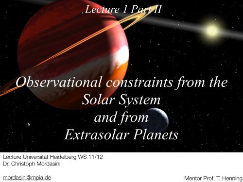
Observational constraints from the
Lecture Universität Heidelberg WS 11/12
Dr. Christoph Mordasini
Lecture 1 Part II
Solar System
and from
Extrasolar Planets
mordasini@mpia.de Mentor Prof. T. Henning

1. Introduction
Lecture overview
2. Planet formation paradigm
3. Structure of the Solar System
4. The surprise: 51 Peg b
5. Detection techniques: radial velocity, transits,
direct imaging, (microlensing, timing, astrometry)
6. Properties of extrasolar planets: mass, distance,
eccentricity distributions, metallicity effect, mass-
radius diagram, ...

6. Properties of extrasolar planets

692 planets
Current status
Candidates detected by radial velocity or astrometry
524 planetary systems
640 planets
76 multiple planet systems
Transiting planets
171 planetary systems
184 planets
14 multiple planet systems
Candidates detected by microlensing
12 planetary systems
13 planets
1 multiple planet systems
Candidates detected by imaging
22 planetary systems
25 planets
1 multiple planet systems
Candidates detected by timing
9 planetary systems
14 planets
4 multiple planet systems
+ 1235 planet candidates from
the KEPLER satellite (transit)
Extra-solar planet encyclopedia (http://exoplanet.eu/)
9.11.2011

Different techniques - different constraints
direct imaging

A quickly progressing field
•Incredible wealth of data provided by already flying space mission (e.g. CoRoT and Kepler).
More to come.
•Field observationally driven. Formation theory struggles to keep up... Observation and theory
often don’t match well.
•Common characteristic: provide observations of a large number of exoplanets. This data
should therefore be treated as a statistical ensemble. This could help.
Venus
Earth
Mars
Jupiter
Saturn
Uranus
Neptune

Overview on observed exoplanet properties
• Extrasolar planets exhibit a very large diversity (all techniques).
• Frequencies -Low mass close-in planets: approx. 50 % (radial velocity)
-Jovian planets inside a few AU: approx. 10-15 % (rv)
-Hot Jupiters: 0.5-1% (rv, transits)
-Cold Neptunes are common (microlensing)
-Overall (FGK stars): any mass, P

Today, formation theory cannot explain all these
observed characteristics in one coherent picture.
But at least for some observations, theory can give us
ideas about possible mechanisms responsible for them.

6.1 a-M diagram

Diversity & structures in the a-M diagram
Radial velocity
& Transits
J. Schneider’s exoplanet.eu
~2010 (already outdated!)
Microlensing
Direct imaging
Diversity
- close-in giant planets
- evaporating planets
- eccentric planets
- super Jupiters
- Hot Neptunes & Super Earth
- pile-ups and voids:
planetary desert
period valley
- planets at large distances
HARPS high
precision
sample 2011

Frequency of planet types
Bias-corrected frequency (at least one planet per star) in the a-M (or equivalently period-mass)
plane found by high precision RV around solar like FGK stars.
Close in planets: P

6.2 Mass distribution

∼15 MJup, with an upper mass limit corresponding to the (vanishing) tail of
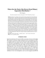
mass distribution. The planet mass distribution is shown in Fig. 1 and follows
wer law, dN/dM ∝ M −1.05 54), 55) affected very little by the unknown sin i. 41)
paucity of companions with Msin i greater than 12 MJup confirms the presence
“brown dwarf desert” 54) for companions with orbital periods up to a decade.
Marcy et al. 2005
Number of Planets
20
15
10
5
Planet Mass Distribution
dN/dM ! M −1.05
104 Planets
Keck, Lick, AAT
0
0 2 4 6 8 10 12 14
M sin i (MJUP) 1. The histogram of 104 planet masses (Msin i) found in the uniform 3 m s −1 Doppler survey
f 1330 stars at Lick, Keck, and the AAT telescopes. The bin size is 0.5 MJup. The distribution
f planet masses rises as M −1.05 from 10 MJup down to Saturn masses, with incompleteness at
ower masses.
Mass distribution: old versions (giants)
•mass distribution from RV observations.
HARPS
•rising towards smaller masses. No obs. bias: smaller masses are more difficult to detect.
•beware of uncorrected (biased) distributions!
•frequency of Jovian planets falls as about M -1 .
•maximum of giant planet masses at about 1 Jupiter mass.
•HARPS gave around 2007 the first hint of a second population of low mass planets.
?
Udry et al. 2007

Mass distribution II: new view (w. low masses)
Mayor et al. 2011
uncorrected for obs. bias corrected for obs. bias
Mayor et al. 2011
•RV: thanks to 1 m/s precision observations, a new huge population of low mass planets
has emerged in the last few years (mostly planets found by HARPS).
•bi (tri?) modal distribution: minimum at about 30 Earth masses. Imprint of formation?
•neptunian bump: strong increase between 30-15 ME.
•overall maximum at small masses
•more than 50% of solar-type stars harbor at least one planet of any mass and with
period up to 100 days (!)

Grether & Lineweaver 2006
Mass distribution III: upper boundary
desert
• less than 0.6 % of Sun-like stars have
a brown-dwarf companion: so called
“Brown dwarf desert”
•mass distribution function shows a
lack of objects between 25-45 MJ.
Upper end of planet mass distribution?
•Nothing particular is seen at 13 MJ (Dburning
limit).
Sahlmann et al. 2010
Segresan et al.
A distinction of BD vs. planets based on formation
seems advisable, but difficult to realize in practice.

6.3 Semimajor axis distribution

ative points of view invoke in situ formation (Bodenheimer, Hubickyj & Lissauer
000), possibly triggered through disk instabilities (Boss 1997, Durisen et al. 2007).
ote however that, even in such cases, subsequent disk-planet interactions leading to
N
20
15
10
5
0
Udry & Santos 2007
dry· Santos
Semimajor axis distribution I: giants
Msini>0.75 MJ
Msini

m Kepler 13
Number of Planets per Star
0.1000
0.0100
0.0010
Transits
P 0 = 1.7 days
P 0 = 2.2 days
0.0001
0.68 1.2 2.0 3.4 5.9 10 17 29 50
Orbital Period (days)
Howard et al. 2011
Semimajor axis distribution II:
P 0 = 7.0 days
low mass/radius planets
2!4 R E
4!8 R E
8!32 R E
ig. 7.— Measured planet occurrence (filled circles) as a funcn
of orbital period with best-fit models (solid curves) overlaid.
ese models are power laws with exponential cutoffs belowachareristic
RVperiod,
P0 (see text and equation 8). P0 increases with
reasing planet radius, suggesting that the migration and parkmechanism
that deposits planets close-in depends on planet
ius. Colors correspond to the same ranges of radii as in Figure
The occurrence measurements (filled circles) are the same as in
ure 6, however for clarity the 2–32 R⊕ measurements and fit
excluded here. As before, only stars in the solar subset (Table
and planets with Rp > 2 R⊕ were used to compute occurrence.
e integrated occurrence to P = 50 days is given in
ble 4.
4. STELLAR EFFECTIVE TEMPERATURE
4.1. Planet Occurrence
n the previous section we considered only GK stars
th properties consistent with those listed in Table 1.
particular, only stars with Teff =4100–6100Kwere
Mayor et al. 2011
ed to compute planet occurrence. Here we expand this
Cut off below P0:
-small radii 2-4 Re: P0 = 7 days
-large radii >4 Re : P0 = 2 days.
Neptunian and smaller sized further out than giant planets.
No pile up at 3 days. Consistent with earlier results from
high precision RV. Lovis et al. 2009 estimated 10 days.
Different stopping mechanism?
Msini

6.4 Eccentricity distribution

Eccentricity distribution
Mayor et al. 2011
•high and even very high eccentricities are common among exoplanets. This is very different
than in the Solar System.
•mean eccentricity for giants: 0.28 > any planet of the Solar System.
•lower mass planets seem to have lower (but still quite high) e 10 MJ), dynamical interactions in a cluster

6.5 Metallicity

Mordasini et al. 2009
Stellar metallicity
•[Fe/H]: iron content of the star ([Fe/H]=0: solar composition, [Fe/H]=0.5: ~ 3 times more
iron than the sun).
•Iron serves as a proxy for the overall metal content in the star (scaled solar composition).
•Stars in the the solar neighborhood have a distribution of metallicities which is roughly
Gaussian around zero.
•Other parts in the galaxies can have completely different [Fe/H] distributions. These stars
can also have a non-scaled solar composition (e.g. thick disk stars).
•There exists also a galactic metallicity gradient (higher [Fe/H] towards the center).

N. Santos et al. (2005)
Metallicity effect for giant planets
search sample (all stars)
stars with giant planets
•the detection probability for giant planets is a strongly increasing function of the host star
metallicity.
•No hot Jupiters found in globular cluster 47 Tuc ([Fe/H]=-0.76). Expected for solar neighborhood
frequency (~0.5%): seven discoveries.
•Best known star-planet correlation for exoplanets. Important constraint for formation.
•Explanation:
• planets form more readily in metal rich systems (primordial hypothesis). Likely.
• falling in planets have enriched the star (pollution hypothesis)

No metallicity effect for low mass planets
Mayor et al. 2011
•HARPS high precision sample: [Fe/H] for giant gaseous planets (black), for planets less
massive than 30 ME (red), and for the global combined sample stars (blue).
•No metallicity effect for low mass planets.
•Even absence of low mass planets at high [Fe/H]?
•Natural outcome in the core accretion formation model.
?
?
Mayor et al. 2011

Sousa et al. 2011
Metallicity effect as function of mass
•The division between metalophile and not
metalophile planets coincides with a minimum in
the planetary mass function. (ca. 30 ME)
•Different populations: Giant planets (w. gas
runaway accretion) vs. Neptunian planets.
•Correlation with other elemental abundances in
the stars are less clear (maybe Lithium-planet
anticorrelation).

6.6 Stellar mass

Influence of the host star mass
•Equal bin in log(Mstar)
• M dwarfs
• solar stars
• intermediate masses
•Planetary system mass / star number
=> mass of planetary material scales with
Mstar
•Planets around more massive stars are
more massive and more frequent.
•RV bias underestimate the last bin.
•The Neptunian vs Jovian planet ratio is
higher around M dwarfs.
•Consistent with a correlation of stellar
mass, protoplanetary disk mass, and
(giant) planet formation probability.

6.7 Multiplicity

Multiplicity
•Fraction of giant planets in multiple systems: ~25%. Incomplete...
•Fraction of low mass planets in multiple systems: ~70%
•Hot Jupiters seem to be lonely. Formation? Disk cleaning? Kozai?
•HD10180: up to 7 planets (RV)
HD10180 a[AU] Msini
(b) 0.02 1.4
c 0.06 13.2
d 0.13 11.9
e 0.27 25.4
f 0.49 23.6
g 1.4 21.4
h 3.4 65.3
Lovis et al. 2011
•Eccentricities 0-0.15
•Solar like star Fe/H=0.08, M=1.06 Msun
•Some period ratios are fairly close to integer or
half-integer values, but no mean-motion
resonances.
•Roughly regularly spaced on a logarithmic scale
•Kepler-11: six transiting planets
Kepler-11 a[AU] Msini
b 0.09 4.3
c 0.11 13.5
d 0.15 6.1
e 0.19 8.4
f 0.25 2.3
g 0.46

numbers=distance in mutual Hill spheres.
Packed systems
Lovis et al. 2011
•Low mass planets seem to follow a radius exclusion law: they cannot be too close together
when measured in mutual Hill spheres.
•Many systems seem to be dynamically packed. Could not add another planet.
•Numerical simulations show that systems with 3–5 planets and masses between a few ME
and a few MJ, separations between adjacent planets should be of at least 7–9 mutual Hill radii
to ensure stability on a 10-Gyr timescale.
•Additional stability islands exist at resonances.
•Dynamical evolution of the systems. Ejection/collision of surplus planets.

Kepler multiple systems
•Kepler has detected a lot of systems with multiple
1
transiting planet candidates.
•The distribution of observed period ratios shows
0.6
that the majority of candidate pairs are neither in nor
near low-order mean motion resonances. 0.4
•Nonetheless, there is a small but statistically
0
significant excesses of pairs both in resonance and
spaced slightly further apart, particularly near 2:1.
N/N TOT
N/N TOT < 5
•Resonant capture due during migration?
Lissauer et al. 2011
1
0
1 1.5 2 2.5 3 3.5 4 4.5 5
0.8
0.2
Slope of Cumulative Period Ratio
500
450
400
350
300
250
200
150
100
Period Ratio
Kepler adjacent pairings
RV adjacent pairings
1 10 100
50
Period Ratio
Kepler adjacent pairings
RV adjacent pairings
Fig. 6.— Cumulative fraction of neighboring planet pairs for Kepler candidate multiplanet sy
–46–
Kepler adjacent pairings
RV adjacent pairings
0
1 1.5 2 2.5 3
Period Ratio
3.5 4 4.5 5
Fig. 7.— Slope of the cumulative fraction of Kepler neighboring planet pairs (solid black curve) an
multiplanet systems detected via radial velocity (dashed red curve) with period ratio exceeding th

6.8 Radius distribution

or stems directly from 35% rms uncertainty
the KIC, which propagates directly to 35%
in Rp. We assumed a central transit over
ar diameter in equation (2). For randomly
Planet Occurrence from Kepler 9
Planet Occurrence ! d
0.001 0.002 0.004 0.0079 0.016 0.032 0.063 0.13 0.25 0.50 1.0
2 ransiting orientations, the f/dlogP/dlogR average duration
p
π/4 times the duration of a central transit.
0.000035 0.00007 0.00014 0.00028 0.00056 0.0011 0.0022 0.0044 0.0088 0.018 0.035
rrection reduces our Planet Occurrence SNR! in fcell equation (1) by
32
π/4, i.e. a true signal-to-noise ratio threshtead
of 10.0. This is still a very conservative
1 (9) 0.0042
1 (15) 0.0075
1 (52) 0.026
58036 0.00015
58030 0.00026
58020 0.00090
16 reshold. Additionally, our method does not
2 (11) 0.0054 4 (39) 0.019 6 (69) 0.034 1 (15) 0.0071 1 (28) 0.014 1 (25) 0.012 3 (168) 0.082
58031 0.00019 58028 0.00067 58022 0.0012 58017 0.00025 58009 0.00049 58004 0.00043 57997 0.0029
the small fraction of transits that are graz-
e reduced 1 (2) 0.0010 significance. 1 (6) 0.0029 4 (34) 0.017 3 (25) 0.012 1 (15) We 0.0076 3 (70) assumed 0.034 4 (154) 0.076 perfect
58018 0.00004 58009 0.00010 58004 0.00058 57998 0.00043 57988 0.00027 57981 0.0012 57963 0.0026
8
r σCDPP values computed for 3 hr intervals.
Planet Radius, R p (R E)
1 (6) 0.0029 1 (9) 0.0044 7 (73) 0.036 4 (74) 0.037 2 (31) 0.015 4 (160) 0.079 5 (278) 0.14
57982 0.00010 57967 0.00015 57942 0.0012 57903 0.0013 57859 0.00053 57804 0.0028 57738 0.0048
derestimate σCDPP for a 6 hr interval (ap-
1 (4) 0.0021
4 (45) 0.022 2 (18) 0.0087 4 (60) 0.030 5 (153) 0.076 6 (208) 0.10 5 (198) 0.099
57907 0.00007
57808 0.00078 57749 0.00030 57653 0.0010 57538 0.0027 57429 0.0036 57240 0.0035
the duration 4 of a P = 50 day transit) by
3 (20) 0.010 9 (104) 0.052 21 (353) 0.18 23 (607) 0.31 16 (591) 0.30 17 (799) 0.43
se are minor corrections 57442 0.00035 57262 0.0018 57001 0.0062 and 56605 0.011 affect 55834 0.011 54371 the 0.015 nu-
denominator of equation (2) nearly equally.
2
3 (21)
56665
0.011 7 (64)
0.00037 55966
0.032 21 (269)
0.0011 54585
0.15 31 (521)
0.0051 52260
0.30 36 (893)
0.010 48639
0.53 34 (1101)
0.019 43318
0.79 18 (749)
0.028 36296
1 (5) 0.0026 3 (17) 0.012 11 (85) 0.060 19 (262) 0.22 11 (159) 0.16 16 (375) 0.43 12 (410) 0.83 7 (295) 0.76
urrence 52618 as 0.00009 49170 a 0.00042 Function 44059 0.0021 37278 0.0079 29498 of 0.0056 Planet 21606 0.015 14712 Radius
0.029 9157 0.027
0.61
0.021
Number o
Kepler
0.001
results
Number of Planets per Star with P < 50 days
1.0 1.4 2.0 2.8 4.0 5.7 8.0 11.3 16.0 22.6
Planet Radius (RE) 3 (10) 0.0075 1 (10) 0.011 4 (50) 0.067 6 (59) 0.22 1 (18) 0.062 3 (85) 0.81 2 (41) 0.95
1 30446 0.00026 22540 0.00040 15445 0.0023 9764 0.0077 5784 0.0022 3170 0.028 1605 0.033
0.68 1.2 2.0 3.4 5.9 10 17 29 50
Orbital Period, P (days)
Fig. 4.— Planet occurrence as a function of planet radius and orbital period for P 10 are shown as black dots. The phase space is divided into a grid of logarithmically spaced cells within which planet occurrence
is computed. Only stars in the “solar subset” (see selection criteria in Table 1) were used to compute occurrence. Cell color indicates
planet occurrence with the color scale on the top in two sets of units,occurrencepercellandoccurrenceperlogarithmicarea unit. White
cells contain no detected planets. Planet occurrence measurements are incomplete and likely contain systematic errors inthehatched
region (Rp < 2 R⊕). Annotations in white text within each cell list occurrence statistics: upper left—the number of detected planets
with SNR > 10, npl,cell, andinparenthesesthenumberofaugmentedplanetscorrecting for non-transiting geometries, npl,aug,cell; lower
left—the number of stars surveyed by Kepler around which a hypothetical transiting planet with Rp and P values from the middle of the
cell could be detected with SNR > 10; lower right—fcell, planetoccurrence,correctedforgeometryanddetectionincompleteness; upper
right—d2 urrence varies by three orders of magnitude
0.00
s-period plane (Figure 4). To isolate the de- Howard et al. 2011
these parameters, we first considered planet
Planet Radius (RE) s•Only a function reliable of planet KEPLER radius, candidates marginalizing around bright, main sequence GK stars.
ets f/dlog10 P/dlog10 Rp, planetoccurrenceperlogarithmicareaunit(dlog10 P dlog10 Rp =28.5gridcells).
•Correct with P for < observational 50 days. We computed bias. Complete oc- to p=50 d, and R > 2 RE.
ng equation (2)
•decrease with
for cells
period
with the ranges of
re 4 but for all periods less than 50 days.
valent •decrease to summing with the size occurrence (S/N) values in
ng•Diagonal rows of cells band to obtain of increasing the occurrence planet frequency. for
n a radius interval with P < 50 days. The
tribution •Strong
of
increase
planet radii
towards
(Figure
small
5) increases
radius. Reminiscent of RV results.
with •But decreasing absolute fraction Rp. less than HARPS. Radius - mass relationship? Does HARPS detect high
eddensity this distribution planets that of planet KEPLER occurrence cannot with see?
0.12
0.10
0.08
0.06
0.04
0.02
Incompleteness
1.0 1.4 2.0 2.8 4.0 5.7 8.0 11.3 16.0 22.6
Fig. 5.— Planet occurrence as a function of planet radius for
planets with P

6.9 Mass-Radius diagram

M-R: Giant planets
•During evolution on Gyrs, giant planets contract and cool.
•The more massive the core, the smaller the total radius.
•Many transiting Hot Jupiters are bloated planets: not explainable by standard
internal structure modeling. Energy source must act deep in the interior. Several
mechanism proposed for explanation.
•Some giant exoplanets seem to contain very large amounts of metals (>100 ME)

M-R: Low mass planets
Kepler-11 b,c,d,e,f
Kepler 10b
Corot-7b
•Diversity: very different radii for a given M. Some are clearly rocky planets.
•Observational constraints on the internal composition.
•Migration?
•Problem: degeneracy. different composition can give the same M-R.
•e.g. Ice=rock + some H2/He. Spectra of atmospheres can help to distinguish: Water vapor
atmosphere has a smaller scale height than a H2/He atmosphere.
•Close in planets! Evaporation (atmospheric escape) could play an important role on Gyrs.
•Must consider formation and evolution.
•Origin unknown... low mass planets from the beginning or boiled down giant planets?

Additional observations

Direct imaging: planets form hot
Janson et al. 2011
•The two competing models
for giant planet formation, core
accretion and direct collapse,
predict different initial
conditions for planet evolution.
•For direct collapse, planets
should initially be very hot.
•For core accretion, they can
also be cold.
•Observations point to a “Hot
start”.
•This could help to distinguish
formation models.

Transits: correlation planetary core mass
Guillot et al.
and stellar metallicity
•Transit observations & RV mass measurements show that the core mass
of giant planets, and the stellar metallicity are positively correlated.
•This is reproduced by core accretion models.
•Recent observations maybe even indicate that that all giant planets
contain at least 10 ME of metals.
•For direct collapse, planets can result both enriched and depleted.
Miller & Fortney 2010

Questions?