CHAPTER 13 C Level Questions 1. In the sticky-price model ...
CHAPTER 13 C Level Questions 1. In the sticky-price model ...
CHAPTER 13 C Level Questions 1. In the sticky-price model ...

You also want an ePaper? Increase the reach of your titles
YUMPU automatically turns print PDFs into web optimized ePapers that Google loves.
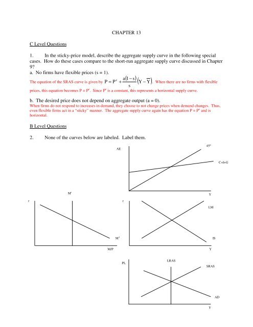
<strong>CHAPTER</strong> <strong>13</strong>C <strong>Level</strong> <strong>Questions</strong><strong>1.</strong> <strong>In</strong> <strong>the</strong> <strong>sticky</strong>-<strong>price</strong> <strong>model</strong>, describe <strong>the</strong> aggregate supply curve in <strong>the</strong> following specialcases. How do <strong>the</strong>se cases compare to <strong>the</strong> short-run aggregate supply curve discussed in Chapter9?a. No firms have flexible <strong>price</strong>s (s = 1).( ) e a 1−sThe equation of <strong>the</strong> SRAS curve is given by P = P + ( Y − Y). When <strong>the</strong>re are no firms with flexibles<strong>price</strong>s, this equation becomes P = P e . Since P e is a constant, this represents a horizontal supply curve.b. The desired <strong>price</strong> does not depend on aggregate output (a = 0).When firms do not respond to increases in demand, <strong>the</strong>y choose to not change <strong>price</strong>s when demand changes. Thus,even flexible firms act in a “<strong>sticky</strong>” manner. The aggregate supply curve again has <strong>the</strong> equation P = P e and ishorizontal.B <strong>Level</strong> <strong>Questions</strong>2. None of <strong>the</strong> curves below are labeled. Label <strong>the</strong>m.AE45°C+I+GM sYM dSRASrrLMISM/PYPLLRASADY
. Since George Bush has taken office, government expenditures on goods and services hasincreased at a rapid pace. On <strong>the</strong> above diagrams, demonstrate <strong>the</strong> impact of this increase ingovernment spending. <strong>In</strong> order from <strong>the</strong> beginning of <strong>the</strong> short run to <strong>the</strong> end of <strong>the</strong> long run,number <strong>the</strong> changes to your diagram (1 is <strong>the</strong> first change, 2 <strong>the</strong> next, etc.).Because it is difficult to fit all changes on one graph, I have reproduced two graphs. The first shows <strong>the</strong> transition to<strong>the</strong> short run equilibrium and <strong>the</strong> second demonstrates <strong>the</strong> transition from <strong>the</strong> short-run to <strong>the</strong> long-run equilibrium.
c. Assume that this economy has population growth of 2% per year and technological growth of1% per year. On <strong>the</strong> plots below, draw <strong>the</strong> impact of <strong>the</strong> increased government expendituresover time. Be sure to indicate what was happening in <strong>the</strong> economy before <strong>the</strong> change inexpenditures (which occurred at time t 0 ), in <strong>the</strong> short run (which ends at time t 1 ), in <strong>the</strong> long run(which ends at time t 2 ), and <strong>the</strong>n after <strong>the</strong> long run equilibrium has been achieved. (20)RGDPPLTimerTimeiTime<strong>In</strong>ventoriest 0 t 1 t 2TimeTime
d. Imagine that <strong>the</strong> short run aggregate supply curve is upward sloping because firm ownerscannot perfectly identify a relative versus absolute change in demand. Given this setup, list, inorder, <strong>the</strong> chain of events in <strong>the</strong> economy given <strong>the</strong> higher amounts of government spending.Continue your chain of events to include both <strong>the</strong> short and <strong>the</strong> long runs (you can use symbolsinstead of sentences). I'll be happy to help you out by starting:SR: G↑ → AE↑ → Y d ↑ → IS↑ → M d ↑ → r↑ → AD↑ → P↑ → W↑ → L↑ → RGDP↑LR: W↓ → L↓ → RGDP↓ →P↑ →M s ↓ → r↑ →I↓ → AE↓ → Y d ↓e. Upon examining your answers to parts a-d of this question, it should become apparent that,given a change in government spending, that RGDP changes by a different amount in <strong>the</strong> shortrun. For a given change in government spending, what factors influence <strong>the</strong> amount of change inRGDP?The slopes of <strong>the</strong> SRAS, <strong>the</strong> LM, and <strong>the</strong> AE curves.A <strong>Level</strong> <strong>Questions</strong>3. a. Suppose that <strong>the</strong> short run aggregate supply curve is upward sloping because of <strong>sticky</strong>wages. Suppose fur<strong>the</strong>r that labor contracts specify that <strong>the</strong> nominal wage be fully indexed forinflation as measured by <strong>the</strong> CPI. That is, <strong>the</strong> nominal wage is to be adjusted to fullycompensate for changes in <strong>the</strong> consumer <strong>price</strong> index. How does this indexation alter <strong>the</strong> shortrun aggregate supply curve?The SRAS curve becomes perfectly vertical (thus, it becomes <strong>the</strong> LRAS).b. Over <strong>the</strong> last 10 years, a number of economists have pointed out that, because of <strong>the</strong> way it ismeasured, <strong>the</strong> CPI actually overstates <strong>the</strong> level of inflation that an economy experiences. If thisis <strong>the</strong> case and wages are indexed by <strong>the</strong> CPI, what shape/slope would <strong>the</strong> short run aggregatesupply curve have?The SRAS has a negative slope.Do Problems and Applications #2 – 7 on pp. 373-374 on Mankiw.