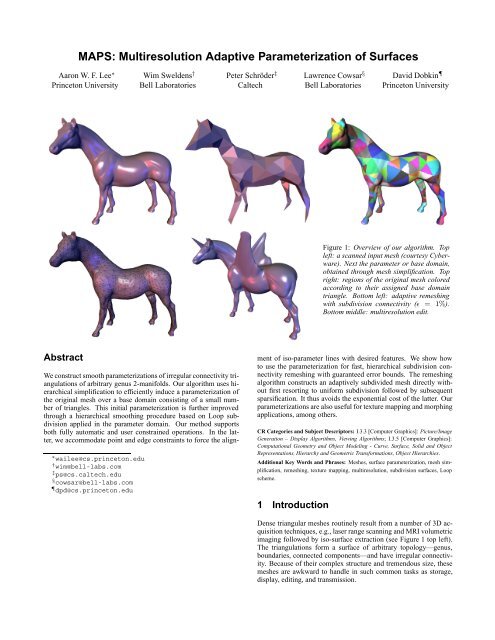
MAPS: Multiresolution Adaptive Parameterization of Surfaces

Vertex removal followed by retriangulationHalf edge collapse as vertex removal with special retriangulationMesh at level l Mesh at level l-1General Edge collapse operationFigure 2: Examples of different atomic mesh simplification steps. Atthe top vertex removal, in the middle half-edge collapse, and edgecollapse at the bottom.algorithm randomly selects a non-marked vertex of outdegree lessthan 12, removes it and its star from K l , marks its neighbors asunremovable and iterates this until no further vertices can be removed.In a triangulated surface the average outdegree of a vertexis 6. Consequently, no more than half of the vertices can be of outdegree12 or more. Thus it is guaranteed that at least 1/24 of thevertices will be removed at each level [5]. In practice, it turns outone can remove roughly 1/4 of the vertices reflecting the fact thatthe graph is four-colorable. Given that a constant fraction can beremoved on each level, the number of levels behaves as O(log N).The entire hierarchy can thus be constructed in linear time.In our approach, we stay in the DK framework, but replace therandom selection of vertices by a priority queue based on geometricinformation. Roughly speaking, vertices with small and flat 1-ringneighborhoods will be chosen first. At level l, for a vertex p i ∈P l , we consider its 1-ring neighborhood ϕ(|star (i)|) and computeits area a(i) and estimate its curvature κ(i). These quantities arecomputed relative to K l , the current level. We assign a priority to{i} inversely proportional to a convex combination of relative areaand curvaturea(i)κ(i)w(λ, i) =λ+(1− λ)max pi ∈Pl a(i) max pi ∈P l κ(i) .(We found λ =1/2 to work well in our experiments.) Omitting allvertices of outdegree greater than 12 from the queue, removal of aconstant fraction of vertices is still guaranteed. Because of the sortimplied by the priority queue, the complexity of building the entirehierarchy grows to O(N log N).Figure 4 shows three stages (original, intermediary, coarsest) ofthe DK hierarchy. Given that the coarsest mesh is homeomorphicto the original mesh, it can be used as the domain of a parameterization.Figure 3: On the left a mesh with a maximally independent set ofvertices marked by heavy dots. Each vertex in the independent sethas its respective star highlighted. Note that the star ’s of the independentset do not tile the mesh (two triangles are left white). Theright side gives the retriangulation after vertex removal.2.4 Flattening and RetriangulationTo find K l−1 , we need to retriangulate the holes left by removingthe independent set. One possibility is to find a plane into which toproject the 1-ring neighborhood ϕ(|star (i)|) of a removed vertexϕ(|i|) without overlapping triangles and then retriangulate the holein that plane. However, finding such a plane, which may not evenexist, can be expensive and involves linear programming [4].Instead, we use the conformal map z a [6] which minimizes metricdistortion to map the neighborhood of a removed vertex into theplane. Let {i} be a vertex to be removed. Enumerate cyclicallythe K i vertices in the 1-ring N (i) ={j k | 1 ≤ k ≤ K i} suchthat {j k−1 ,i,j k } ∈ K l with j 0 = j Ki . A piecewise linear approximationof z a , which we denote by µ i, is defined by its valuesfor the center point and 1-ring neighbors; namely, µ i(p i)=0andµ i(p jk )=rk a exp(iθ k a), where r k = ‖p i − p jk ‖,k∑θ k = ̸ (p jl−1 ,p i,p jl ),l=1and a =2π/θ Ki . The advantages of the conformal map are numerous:it always exists, it is easy to compute, it minimizes metricdistortion, and it is a bijection and thus never maps two triangles ontop of each other. Once the 1-ring is flattened, we can retriangulatethe hole using, for example, a constrained Delaunay triangulation(CDT) (see Figure 5). This tells us how to build K l−1 .When the vertex to be removed is a boundary vertex, we map to ahalf disk by setting a = π/θ Ki (assuming j 1 and j Ki are boundaryvertices and setting θ 1 =0). Retriangulation is again performedwith a CDT.3 Initial ParameterizationTo find a parameterization, we begin by constructing a bijectionΠ from ϕ(|K L |) to ϕ(|K 0 |). The parameterization of the originalmesh over the base domain follows from Π −1 (ϕ(|K 0 |)). In otherwords, the mapping of a point p ∈ ϕ(|K L |) through Π is a pointp 0 =Π(v) ∈ ϕ(|K 0 |), which can be written asp 0 = αp i + βp j + γp k ,where {i, j, k} ∈K 0 is a face of the base domain and α, β and γare barycentric coordinates, i.e., α + β + γ =1.

Original mesh (level 14)3 spaceFlattening into parameter planeIntermediate mesh (level 6)retriangulationFigure 5: In order to remove a vertex p i, its star (i) is mapped from3-space to a plane using the map z a . In the plane the central vertexis removed and the resulting hole retriangulated (bottom right).Coarsest mesh (level 0)kassign barycentriccoordinates to oldpoint in new trianglejFigure 4: Example of a modified DK mesh hierarchy. At the topthe finest (original) mesh ϕ(|K L |) followed by an intermediatemesh, and the coarsest (base) mesh ϕ(|K 0 |) at the bottom (originaldataset courtesy University of Washington).The mapping can be computed concurrently with the hierarchyconstruction. The basic idea is to successively compute piecewiselinear bijections Π l between ϕ(|K L |) and ϕ(|K l |) starting withΠ L , which is the identity, and ending with Π 0 =Π.Notice that we only need to compute the value of Π l at the verticesof K L . At any other point it follows from piecewise linearity. 1Assume we are given Π l and want to compute Π l−1 . Each vertex{i} ∈K L falls into one of the following categories:1. {i} ∈K l−1 : The vertex is not removed on level l and surviveson level l − 1. In this case nothing needs to be done.Π l−1 (p i)=Π l (p i)=p i.2. {i} ∈K l \K l−1 : The vertex gets removed when going froml to l − 1. Consider the flattening of the 1-ring around p i (seeFigure 5). After retriangulation, the origin lies in a trianglewhich corresponds to some face t = {j, k, m} ∈K l−1 andhas barycentric coordinates (α,β,γ) with respect to the verticesof that face, i.e., αµ i(p j)+βµ i(p k )+γµ i(p m) (seeFigure 6). In that case, let Π l−1 (p i)=αp j + βp k + γp m.3. {i} ∈ K L \K l : The vertex was removed earlier, thus1 In the vicinity of vertices in K l a triangle {i, j, k} ∈K L can straddlemultiple triangles in K l . In this case the map depends on the flatteningstrategy used (see Section 2.4).mFigure 6: After retriangulation of a hole in the plane (see Figure 5),the just removed vertex gets assigned barycentric coordinates withrespect to the containing triangle on the coarser level. Similarly, allthe finest level vertices that were mapped to a triangle of the holenow need to be reassigned to a triangle of the coarser level.Π l (p i)=α ′ p j ′ + β ′ p k ′ + γ ′ p m ′ for some triangle t ′ ={j ′ ,k ′ ,m ′ } ∈ K l . If t ′ ∈ K l−1 , nothing needs to bedone; otherwise, the independent set guarantees that exactlyone vertex of t ′ is removed, say {j ′ }. Consider theconformal map µ j ′ (Figure 6). After retriangulation, theµ j ′(p i) lies in a triangle which corresponds to some facet = {j, k, m} ∈K l−1 with barycentric coordinates (α,β,γ)(black dots within highlighted face in Figure 6). In that case,let Π l−1 (p i)=αp j + βp k + γp m (i.e., all vertices in Figure6 are reparameterized in this way).Note that on every level, the algorithm requires a sweep through allthe vertices of the finest level resulting in an overall complexity ofO(N log N).Figure 7 visualizes the mapping we just computed. For eachpoint p i from the original mesh, its mapping Π(p i) is shown with adot on the base domain.Caution: Given that every association between a 1-ring and itsretriangulated hole is a bijection, so is the mapping Π. However,Π does not necessarily map a finest level triangle to a triangularregion in the base domain. Instead the image of a triangle may bea non-convex region. In that case connecting the mapped verticeswith straight lines can cause flipping, i.e., triangles may end up on

3 spaceFlattening into parameter planeFigure 7: Base domain ϕ(|K 0 |). For each point p i from the originalmesh, its mapping Π(p i) is shown with a dot on the base domain.top of each other (see Figure 8 for an example). Two methods existfor dealing with this problem. First one could further subdividethe original mesh in the problem regions. Given that the underlyingcontinuous map is a bijection, this is guaranteed to fix the problem.The alternative is to use some brute force triangle unflippingmechanism. We have found the following scheme to work well:adjust the parameter values of every vertex whose 2-neighborhoodcontains a flipped triangle, by replacing them with the averaged parametervalues of its 1-ring neighbors [7].original meshmapping onto base domainimage of verticesimage of triangleFigure 8: Although the mapping Π from the original mesh to abase domain triangle is a bijection, triangles do not in generalget mapped to triangles. Three vertices of the original mesh getmapped to a concave configuration on the base domain, causingthe piecewise linear approximation of the map to flip the triangle.retriangulationFigure 9: When a vertex with two incident feature edges is removed,we want to ensure that the subsequent retriangulation adds a newfeature edge to replace the two old ones.{v i,v i+1} along the x-axis, and use two boundary type conformalmaps to the half disk above and below (cf. the last paragraph ofSection 2.4). When retriangulating the hole around v i, we put theedge {v i−1,v i+1} in K l−1 , tag it as a feature edge, and computea CDT on the upper and lower parts (see Figure 9). If we applysimilar procedures on coarser levels, we ensure that v 1 and v I remainconnected by a path (potentially a single edge) on the basedomain. This guarantees that Π maps the curved feature path ontothe coarsest level edge(s) between v 1 and v I.In general, there will be multiple feature paths which may beclosed or cross each other. As usual, a vertex with more than 2incident feature edges is considered a corner, and marked as unremovable.The feature vertices and paths can be provided by the user ordetected automatically. As an example of the latter case, we considerevery edge whose dihedral angle is below a certain thresholdto be a feature edge, and every vertex whose curvature is above acertain threshold to be a feature vertex. An example of this strategyis illustrated in Figure 13.3.1 Tagging and Feature LinesIn the algorithm described so far, there is no a priori control overwhich vertices end up in the base domain or how they will be connected.However, often there are features which one wants to preservein the base domain. These features can either be detectedautomatically or specified by the user.We consider two types of features on the finest mesh: verticesand paths of edges. Guaranteeing that a certain vertex of the originalmesh ends up in the base domain is straightforward. Simplymark that vertex as unremovable throughout the DK hierarchy.We now describe an algorithm to guarantee that a certain path ofedges on the finest mesh gets mapped to an edge of the base domain.Let {v i | 1 ≤ i ≤ I} ⊂K L be a set of vertices on thefinest level which form a path, i.e., {v i,v i+1} is an edge. Tag allthe edges in the path as feature edges. First tag v 1 and v I, so calleddart points [14], as unremovable so they are guaranteed to end upin the base domain. Let v i be the first vertex on the interior of thepath which gets marked for removal in the DK hierarchy, say, whengoing from level l to l − 1. Because of the independent set property,v i−1 and v i+1 cannot be removed and therefore must belong toK l−1 . When flattening the hole around v i, tagged edges are treatedlike a boundary. We first straighten out the edges {v i−1,v i} and3.2 A Quick ReviewBefore we consider the problem of remeshing, it may be helpfulto review what we have at this point. We have established an initialbijection Π of the original surface ϕ(|K L |) onto a base domainϕ(|K 0 |) consisting of a small number of triangles (e.g. Figure 7).We use a simplification hierarchy (Figure 4) in which the holes aftervertex removal are flattened and retriangulated (Figures 5 and 9).Original mesh points get successively reparametrized over coarsertriangulations (Figure 6). The resulting mapping is always a bijection;triangle flipping (Figure 8) is possible but can be corrected.4 RemeshingIn this section, we consider remeshing using subdivision connectivitytriangulations since it is both a convenient way to illustrate theproperties of a parameterization and is an important subject in itsown right. In the process, we compute a smoothed version of ourinitial parameterization. We also show how to efficiently constructan adaptive remeshing with guaranteed error bounds.

4.1 Uniform RemeshingSince Π is a bijection, we can use Π −1 to map the base domainto the original mesh. We follow the strategy used in [7]: regularly(1:4) subdivide the base domain and use the inverse map toobtain a regular connectivity remeshing. This introduces a hierarchyof regular meshes (Q m , R m ) (Q is the point set and R is thecomplex) obtained from m-fold midpoint subdivision of the basedomain (P 0 , K 0 )=(Q 0 , R 0 ). Midpoint subdivision implies thatall new domain points lie in the base domain, Q m ⊂ ϕ(|R 0 |) and|R m | = |R 0 |. All vertices of R m \R 0 have outdegree 6. Theuniform remeshing of the original mesh on level m is given by(Π −1 (Q m ), R m ).We thus need to compute Π −1 (q) where q is a point in the basedomain with dyadic barycentric coordinates. In particular, we needto compute which triangle of ϕ(|K L |) contains Π −1 (q), or, equivalently,which triangle of Π(ϕ(|K L |)) contains q. This is a standardpoint location problem in an irregular triangulation. We usethe point location algorithm of Brown and Faigle [2] which avoidslooping that can occur with non-Delaunay meshes [10, 9]. Once wehave found the triangle {i, j, k} which contains q, we can write qasq = α Π(p i)+β Π(p j)+γ Π(p k ),and thusΠ −1 (q) =αp i + βp j + γp k ∈ ϕ(|K L |).Figure 10 shows the result of this procedure: a level 3 uniformremeshing of a 3-holed torus using the Π −1 map.A note on complexity: The point location algorithm is essentiallya walk on the finest level mesh with complexity O( √ N). Hierarchicalpoint location algorithms, which have asymptotic complexityO(log N), exist [15] but have a much larger constant. Giventhat we schedule the queries in a systematic order, we almost alwayshave an excellent starting guess and observe a constant number ofsteps. In practice, the finest level “walking” algorithm beats the hierarchicalpoint location algorithms for all meshes we encountered(up to 100K faces).Instead, we use a much simpler and cheaper smoothing techniquebased on Loop subdivision. The main idea is to compute Π −1at a smoothed version of the dyadic points, rather then at the dyadicpoints themselves (which can equivalently be viewed as changingthe parameterization). To that end, we define a map L from the basedomain to itself by the following modification of Loop:• If all the points of the stencil needed for computing either a newpoint or smoothing an old point are inside the same triangle ofthe base domain, we can simply apply the Loop weights and thenew points will be in that same face.• If the stencil stretches across two faces of the base domain, weflatten them out using a “hinge” map at their common edge.We then compute the point’s position in this flattened domainand extract the triangle in which the point lies together with itsbarycentric coordinates.• If the stencil stretches across multiple faces, we use the conformalflattening strategy discussed earlier.Note that the modifications to Loop force L to map the base domainonto the base domain. We emphasize that we do not apply theclassic Loop scheme (which would produce a “blobby” version ofthe base domain). Nor are the surface approximations that we laterproduce Loop surfaces.The composite map Π −1 ◦Lis our smoothed parameterizationthat maps the base domain onto the original surface. The m-thlevel of uniform remeshing with the smoothed parameterization is(Π −1 ◦L(Q m ), R m ), where Q m , as before, are the dyadic pointson the base domain. Figure 11 shows the result of this procedure:a level 3 uniform remeshing of a 3-holed torus using the smoothedparameterization.When the mesh is tagged, we cannot apply smoothing across thetagged edges since this would break the alignment with the features.Therefore, we use modified versions of Loop which can deal withcorners, dart points and feature edges [14, 23, 26] (see Figure 13).Figure 10: Remeshing of 3 holed torus using midpoint subdivision.The parameterization is smooth within each base domain triangle,but clearly not across base domain triangles.4.2 Smoothing the ParameterizationIt is clear from Figure 10 that the mapping we used is not smoothacross global edges. One way to obtain global smoothness is toconsider a map that minimizes a global smoothness functional andgoes from ϕ(|K L |) to |K 0 | rather than to ϕ(|K 0 |). This wouldrequire an iterative PDE solver. We have found computation ofmappings to topological realizations that live in a high dimensionalspace to be needlessly cumbersome.Figure 11: The same remeshing of the 3-holed torus as in Figure 10,but this time with respect to a Loop smoothed parameterization.Note: Because the Loop scheme only enters in smoothing the parameterizationthe surface shown is still a sampling of the originalmesh, not a Loop surface approximation of the original.4.3 Adaptive RemeshingOne of the advantages of meshes with subdivision connectivity isthat classical multiresolution and wavelet algorithms can be employed.The standard wavelet algorithms used, e.g., in image compression,start from the finest level, compute the wavelet transform,and then obtain an efficient representation by discarding smallwavelet coefficients. Eck et al. [7, 8] as well as Certain et al. [3] followa similar approach: remesh using a uniformly subdivided gridfollowed by decimation through wavelet thresholding. This has thedrawback that in order to resolve a small local feature on the originalmesh, one may need to subdivide to a very fine level. Each extra

level quadruples the number of triangles, most of which will laterbe decimated using the wavelet procedure. Imagine, e.g., a planewhich is coarsely triangulated except for a narrow spike. Makingthe spike width sufficiently small, the number of levels needed toresolve it can be made arbitrarily high.In this section we present an algorithm which avoids first buildinga full tree and later pruning it. Instead, we immediately build theadaptive mesh with a guaranteed conservative error bound. This ispossible because the DK hierarchy contains the information on howmuch subdivision is needed in any given area. Essentially, we letthe irregular DK hierarchy “drive” the adaptive construction of theregular pyramid.We first compute for each triangle t ∈K 0 the following errorquantity:E(t) = max dist(p i,ϕ(|t|)).p i ∈P L and Π(p i )∈ϕ(|t|)This measures the distance between one triangle in the base domainand the vertices of the finest level mapped to that triangle.The adaptive algorithm is now straightforward. Set a certain relativeerror threshold ɛ. Compute E(t) for all triangles of the basedomain. If E(t)/B, where B is the largest side of the boundingbox, is larger than ɛ, subdivide the domain triangle using the Loopprocedure above. Next, we need to reassign vertices to the trianglesof level m =1. This is done as follows: For each point p i ∈P Lconsider the triangle t of K 0 to which it it is currently assigned.Next consider the 4 children of t on level 1, t j with j =0, 1, 2, 3and compute the distance between p i and each of the ϕ(|t j|). Assignp i to the closest child. Once the finest level vertices have beenreassigned to level 1 triangles, the errors for those triangles can becomputed. Now iterate this procedure until all triangles have anerror below the threshold. Because all errors are computed fromthe finest level, we are guaranteed to resolve all features within theerror bound. Note that we are not computing the true distance betweenthe original vertices and a given approximation, but rather aneasy to compute upper bound for it.In order to be able to compute the Loop smoothing map L onan adaptively subdivided grid, the grid needs to satisfy a vertex restrictioncriterion, i.e., if a vertex has a triangle incident to it withdepth i, then it must have a complete 1-ring at level i − 1 [28]. Thisrestriction may necessitate subdividing some triangles even if theyare below the error threshold. Examples of adaptive remeshing canbe seen in Figure 1 (lower left), Figure 12, and Figure 13.ones. The application was written in C++ using standard computationalgeometry data structures, see e.g. [21], and all timings reportedin this section were measured on a 200 MHz PentiumPropersonal computer.Figure 13: Left (top to bottom): three levels in the DK pyramid,finest (L =15) with 12946, intermediate (l =8) with 1530, andcoarsest (l =0) with 168 triangles. Feature edges, dart and cornervertices survive on the base domain. Right (bottom to top):adaptive mesh with ɛ =5%and 1120 triangles (bottom), ɛ =1%and 3430 triangles (middle), and uniform level 3 (top). (Originaldataset courtesy University of Washington.)Figure 12: Example remesh of a surface with boundaries.5 ResultsWe have implemented MAPS as described above and applied it toa number of well known example datasets, as well as some newThe first example used throughout the text is the 3-holed torus.The original mesh contained 11776 faces. These were reduced inthe DK hierarchy to 120 faces over 14 levels implying an averageremoval of 30% of the faces on a given level. The remesh of Figure11 used 4 levels of uniform subdivision for a total of 30720triangles.The original sampled geometry of the 3-holed torus is smoothand did not involve any feature constraints. A more challengingcase is presented by the fandisk shown in Figure 13. The originalmesh (top left) contains 12946 triangles which were reduced to 168

Figure 14: Example of a constrained parameterization based on user input. Top: original input mesh (100000 triangles) with edge tagssuperimposed in red, green lines show some smooth iso-parameter lines of our parameterization. The middle shows an adaptive subdivisionconnectivity remesh. The bottom one patches corresponding to the eye regions (right eye was constrained, left eye was not) are highlighted toindicate the resulting alignment of top level patches with the feature lines. (Dataset courtesy Cyberware.)faces in the base domain over 15 levels (25% average face removalper level). The initial mesh had all edges with dihedral angles below75 o tagged (1487 edges), resulting in 141 tagged edges at thecoarsest level. Adaptive remeshing to within ɛ =5%and ɛ =1%(fraction of longest bounding box side) error results in the meshesshown in the right column. The top right image shows a uniformresampling to level 3, in effect showing iso-parameter lines of theparameterization used for remeshing. Note how the iso-parameterlines conform perfectly to the initially tagged features.This dataset demonstrates one of the advantages of our method—inclusion of feature constraints—over the earlier work of Eck etal. [7]. In the original PM paper [12, Figure 12], Hoppe shows thesimplification of the fandisk based on Eck’s algorithm which doesnot use tagging. He points out that the multiresolution approximationis quite poor at low triangle counts and consequently requiresmany triangles to achieve high accuracy. The comparison betweenour Figure 13 and Figure 12 in [12] demonstrates that our multiresolutionalgorithm which incorporates feature tagging solves theseproblems.Another example of constrained parameterization and subsequentadaptive remeshing is shown in Figure 14. The originaldataset (100000 triangles) is shown on the left. The red lines indicateuser supplied feature constraints which may facilitate subsequentanimation. The green lines show some representative isoparameterlines of our parameterization subject to the red featureconstraints. Those can be used for computing texture coordinates.The middle image shows an adaptive subdivision connectivityremesh with 74698 triangles (ɛ =0.5%). On the right wehave highlighted a group of patches, 2 over the right (constrained)eye and 1 over the left (unconstrained) eye. This indicates how usersupplied constraints force domain patches to align with desired features.Other enforced patch boundaries are the eyebrows, centerof the nose, and middle of lips (see red lines in left image). Thisexample illustrates how one places constraints like Krishnamurthyand Levoy [17]. We remove the need in their algorithms to specifythe entire base domain. A user may want to control patch outlinesfor editing in one region (e.g., on the face), but may not care aboutwhat happens in other regions (e.g., the back of the head).We present a final example in Figure 1. The original mesh(96966 triangles) is shown on the top left, with the adaptive, subdivisionconnectivity remesh on the bottom left. This remesh wassubsequently edited in a interactive multiresolution editing system[28] and the result is shown on the bottom middle.6 Conclusions and Future ResearchWe have described an algorithm which establishes smooth parameterizationsfor irregular connectivity, 2-manifold triangular meshesof arbitrary topology. Using a variant of the DK hierarchy construction,we simplify the original mesh and use piecewise linearapproximations of conformal mappings to incrementally build aparameterization of the original mesh over a low face count basedomain. This parameterization is further improved through a hierarchicalsmoothing procedure which is based on Loop smoothing inparameter space. The resulting parameterizations are of high quality,and we demonstrated their utility in an adaptive, subdivisionconnectivity remeshing algorithm that has guaranteed error bounds.The new meshes satisfy the requirements of multiresolution representationswhich generalize classical wavelet representations andare thus of immediate use in applications such as multiresolutionediting and compression. Using edge and vertex constraints, theparameterizations can be forced to respect feature lines of interestwithout requiring specification of the entire patch network.In this paper we have chosen remeshing as the primary applicationto demonstrate the usefulness of the parameterizations we pro-

Dataset Input size Hierarchy Levels P 0 size Remeshing Remesh Output size(triangles) creation (triangles) tolerance creation (triangles)3-hole 11776 18 (s) 14 120 (NA) 8 (s) 30720fandisk 12946 23 (s) 15 168 1% 10 (s) 3430fandisk 12946 23 (s) 15 168 5% 5 (s) 1130head 100000 160 (s) 22 180 0.5% 440 (s) 74698horse 96966 163 (s) 21 254 1% 60 (s) 15684horse 96966 163 (s) 21 254 0.5% 314 (s) 63060Table 1: Selected statistics for the examples discussed in the text. All times are in seconds on a 200 MHz PentiumPro.duce. The resulting meshes may also find application in numericalanalysis algorithms, such as fast multigrid solvers. Clearly thereare many other applications which benefit from smooth parameterizations,e.g., texture mapping and morphing, which would beinteresting to pursue in future work. Because of its independent setselection the standard DK hierarchy creates topologically uniformsimplifications. We have begun to explore how the selection canbe controlled using geometric properties. Alternatively, one coulduse a PM framework to control geometric criteria of simplification.Perhaps the most interesting question for future research is how toincorporate topology changes into the MAPS construction.AcknowledgmentsAaron Lee and David Dobkin were partially supported by NSF Grant CCR-9643913and the US Army Research Office Grant DAAH04-96-1-0181. Aaron Lee was alsopartially supported by a Wu Graduate Fellowship and a Summer Internship at Bell Laboratories,Lucent Technologies. Peter Schröder was partially supported by grants fromthe Intel Corporation, the Sloan Foundation, an NSF CAREER award (ASC-9624957),a MURI (AFOSR F49620-96-1-0471), and Bell Laboratories, Lucent Technologies.Special thanks to Timothy Baker, Ken Clarkson, Tom Duchamp, Tom Funkhouser,Amanda Galtman, and Ralph Howard for many interesting and stimulation discussions.Special thanks also to Andrei Khodakovsky, Louis Thomas, and Gary Wu forinvaluable help in the production of the paper. Our implementation uses the trianglefacet data structure and code of Ernst Mücke.References[1] BAJAJ, C. L., BERNADINI, F.,CHEN, J., AND SCHIKORE, D. R. AutomaticReconstruction of 3D CAD Models. Tech. Rep. 96-015, Purdue University,February 1996.[2] BROWN, P. J. C., AND FAIGLE, C. T. A Robust Efficient Algorithm for PointLocation in Triangulations. Tech. rep., Cambridge University, February 1997.[3] CERTAIN, A., POPOVIĆ, J., DEROSE, T.,DUCHAMP, T.,SALESIN, D., ANDSTUETZLE, W. Interactive Multiresolution Surface Viewing. In ComputerGraphics (SIGGRAPH 96 Proceedings), 91–98, 1996.[4] COHEN, J., MANOCHA, D., AND OLANO, M. Simplifying Polygonal ModelsUsing Successive Mappings. In Proceedings IEEE Visualization 97, 395–402,October 1997.[5] DOBKIN, D., AND KIRKPATRICK, D. A Linear Algorithm for Determining theSeparation of Convex Polyhedra. Journal of Algorithms 6 (1985), 381–392.[6] DUCHAMP, T.,CERTAIN, A., DEROSE, T., AND STUETZLE, W. HierarchicalComputation of PL harmonic Embeddings. Tech. rep., University of Washington,July 1997.[7] ECK, M., DEROSE, T., DUCHAMP, T., HOPPE, H., LOUNSBERY, M., ANDSTUETZLE, W. Multiresolution Analysis of Arbitrary Meshes. In ComputerGraphics (SIGGRAPH 95 Proceedings), 173–182, 1995.[8] ECK, M., AND HOPPE, H. Automatic Reconstruction of B-Spline Surfaces ofArbitrary Topological Type. In Computer Graphics (SIGGRAPH 96 Proceedings),325–334, 1996.[9] GARLAND, M., AND HECKBERT, P. S. Fast Polygonal Approximation of Terrainsand Height Fields. Tech. Rep. CMU-CS-95-181, CS Dept., Carnegie MellonU., September 1995.[10] GUIBAS, L., AND STOLFI, J. Primitives for the Manipulation of General Subdivisionsand the Computation of Voronoi Diagrams. ACM Transactions on Graphics4, 2 (April 1985), 74–123.[11] HECKBERT, P. S., AND GARLAND, M. Survey of Polygonal Surface SimplificationAlgorithms. Tech. rep., Carnegie Mellon University, 1997.[12] HOPPE, H. Progressive Meshes. In Computer Graphics (SIGGRAPH 96 Proceedings),99–108, 1996.[13] HOPPE, H. View-Dependent Refinement of Progressive Meshes. In ComputerGraphics (SIGGRAPH 97 Proceedings), 189–198, 1997.[14] HOPPE, H., DEROSE, T.,DUCHAMP, T.,HALSTEAD, M., JIN, H., MCDON-ALD, J., SCHWEITZER, J., AND STUETZLE, W. Piecewise Smooth SurfaceReconstruction. In Computer Graphics (SIGGRAPH 94 Proceedings), 295–302,1994.[15] KIRKPATRICK, D. Optimal Search in Planar Subdivisions. SIAM J. Comput. 12(1983), 28–35.[16] KLEIN, A., CERTAIN, A., DEROSE, T.,DUCHAMP, T., AND STUETZLE, W.Vertex-based Delaunay Triangulation of Meshes of Arbitrary Topological Type.Tech. rep., University of Washington, July 1997.[17] KRISHNAMURTHY, V., AND LEVOY, M. Fitting Smooth Surfaces to DensePolygon Meshes. In Computer Graphics (SIGGRAPH 96 Proceedings), 313–324, 1996.[18] LOOP, C. Smooth Subdivision Surfaces Based on Triangles. Master’s thesis,University of Utah, Department of Mathematics, 1987.[19] LOUNSBERY, M.Multiresolution Analysis for Surfaces of Arbitrary TopologicalType. PhD thesis, Department of Computer Science, University of Washington,1994.[20] LOUNSBERY, M., DEROSE, T.,AND WARREN, J. Multiresolution Analysis forSurfaces of Arbitrary Topological Type. Transactions on Graphics 16, 1 (January1997), 34–73.[21] MÜCKE, E. P. Shapes and Implementations in Three-Dimensional Geometry.Technical Report UIUCDCS-R-93-1836, University of Illinois at Urbana-Champaign, 1993.[22] SCHRÖDER, P., AND SWELDENS, W. Spherical Wavelets: Efficiently RepresentingFunctions on the Sphere. In Computer Graphics (SIGGRAPH 95 Proceedings),Annual Conference Series, 1995.[23] SCHWEITZER, J. E. Analysis and Application of Subdivision Surfaces. PhDthesis, University of Washington, 1996.[24] SPANIER, E.H.Algebraic Topology. McGraw-Hill, New York, 1966.[25] XIA, J. C., AND VARSHNEY, A. Dynamic View-Dependent Simplification forPolygonal Models. In Proceedings Visualization 96, 327–334, October 1996.[26] ZORIN, D.Subdivision and Multiresolution Surface Representations. PhD thesis,California Institute of Technology, 1997.[27] ZORIN, D., SCHRÖDER, P., AND SWELDENS, W. Interpolating Subdivisionfor Meshes with Arbitrary Topology. In Computer Graphics (SIGGRAPH 96Proceedings), 189–192, 1996.[28] ZORIN, D., SCHRÖDER, P., AND SWELDENS, W. Interactive MultiresolutionMesh Editing. In Computer Graphics (SIGGRAPH 97 Proceedings), 259–268,1997.