Wavelets - Caltech Multi-Res Modeling Group

f[n] = a[n]
0.8
0.6
0.4
0.2
0
-0.2
-0.4
-0.6
H*
G*
a[n/2]
d[n/2]
a[n/4]
H*
a[n/8]
H*
G*
H*
G*
a[1]
d[1]
G*
d[n/4]
SIGGRAPH ’95 Course Notes
d[n/8]
Non-standard Haar Non-standard Flatlet 2
Non-standard Haar
and their Applications
A A A
...
Wavelet coefficients
Non-standard Flatlet 2
(a) B
(b) B ...
(c)
scaling function
wavelet
-0.8
0 50 100 150 200 250 300 350 400
Wavelets
in Computer Graphics
3
2
1
0
-1
-2
Wavelet coefficients
Organizer:
Alain Fournier
University of British Columbia
scaling function
wavelet
-3
0 100 200 300 400 500 600 700

Nothing to do with sea or anything else.
Over and over it vanishes with the wave.
– Shinkichi Takahashi

Lecturers
Michael F. Cohen
Microsoft Research
One Microsoft Way
Redmond, WA 98052
mcohen@microsoft.com
Tony D. DeRose
Department of Computer Science and Engineering FR-35
University of Washington
Seattle, Washington 98195
derose@cs.washington.edu
Alain Fournier
Department of Computer Science
University of British Columbia
2366 Main Mall
Vancouver, British Columbia V6T 1Z4
fournier@cs.ubc.ca
Michael Lounsbery
Alias Research
219 S. Washington St.
P.O. Box 4561
Seattle, WA 98104
louns@ag.alias.com
Leena-Maija Reissell
Department of Computer Science
University of British Columbia
2366 Main Mall
Vancouver, British Columbia V6T 1Z4
reissell@cs.ubc.ca
Peter Schröder
Department of Computer Science
Le Conte 209F
University of South Carolina
Columbia, SC 29208
ps@math.scarolina.edu
Wim Sweldens
Department of Mathematics
University of South Carolina
Columbia, SC 29208
sweldens@math.scarolina.edu

Table of Contents
Preamble – Alain Fournier 1
1 Prolegomenon :::::::::::::::::::::::::::::::::::::::: 1
I Introduction – Alain Fournier 5
1 Scale ::::::::::::::::::::::::::::::::::::::::::::: 5
1.1 Image pyramids ::::::::::::::::::::::::::::::::::: 5
2 Frequency :::::::::::::::::::::::::::::::::::::::::: 7
3 The Walsh transform ::::::::::::::::::::::::::::::::::::: 8
4 Windowed Fourier transforms :::::::::::::::::::::::::::::::: 10
5 Relative Frequency Analysis ::::::::::::::::::::::::::::::::: 12
6 Continuous Wavelet Transform ::::::::::::::::::::::::::::::: 12
7 From Continuous to Discrete and Back ::::::::::::::::::::::::::: 13
7.1 Haar Transform ::::::::::::::::::::::::::::::::::: 13
7.2 Image Pyramids Revisited :::::::::::::::::::::::::::::: 14
7.3 Dyadic Wavelet Transforms ::::::::::::::::::::::::::::: 15
7.4 Discrete Wavelet Transform ::::::::::::::::::::::::::::: 16
7.5 Multiresolution Analysis ::::::::::::::::::::::::::::::: 17
7.6 Constructing Wavelets :::::::::::::::::::::::::::::::: 17
7.7 Matrix Notation ::::::::::::::::::::::::::::::::::: 19
7.8 Multiscale Edge Detection :::::::::::::::::::::::::::::: 19
8 Multi-dimensional Wavelets ::::::::::::::::::::::::::::::::: 20
8.1 Standard Decomposition ::::::::::::::::::::::::::::::: 20
8.2 Non-Standard Decomposition :::::::::::::::::::::::::::: 20
8.3 Quincunx Scheme :::::::::::::::::::::::::::::::::: 21
9 Applications of Wavelets in Graphics :::::::::::::::::::::::::::: 21
9.1 Signal Compression ::::::::::::::::::::::::::::::::: 21
9.2 Modelling of Curves and Surfaces :::::::::::::::::::::::::: 33
9.3 Radiosity Computations ::::::::::::::::::::::::::::::: 33
10 Other Applications :::::::::::::::::::::::::::::::::::::: 33

II Multiresolution and Wavelets – Leena-Maija Reissell 37
1 Introduction ::::::::::::::::::::::::::::::::::::::::: 37
1.1 A recipe for finding wavelet coefficients ::::::::::::::::::::::: 37
1.2 Wavelet decomposition ::::::::::::::::::::::::::::::: 40
1.3 Example of wavelet decomposition ::::::::::::::::::::::::: 41
1.4 From the continuous wavelet transform to more compact representations :::::: 42
2 Multiresolution: definition and basic consequences ::::::::::::::::::::: 43
2.1 Wavelet spaces :::::::::::::::::::::::::::::::::::: 44
2.2 The refinement equation ::::::::::::::::::::::::::::::: 46
2.3 Connection to filtering :::::::::::::::::::::::::::::::: 46
2.4 Obtaining scaling functions by iterated filtering ::::::::::::::::::: 47
3 Requirements on filters for multiresolution ::::::::::::::::::::::::: 52
3.1 Basic requirements for the scaling function ::::::::::::::::::::: 52
3.2 Wavelet definition :::::::::::::::::::::::::::::::::: 53
3.3 Orthonormality ::::::::::::::::::::::::::::::::::: 54
3.4 Summary of necessary conditions for orthonormal multiresolution ::::::::: 55
3.5 Sufficiency of conditions :::::::::::::::::::::::::::::: 56
3.6 Construction of compactly supported orthonormal wavelets :::::::::::: 58
3.7 Some shortcomings of compactly supported orthonormal bases ::::::::::: 61
4 Approximation properties :::::::::::::::::::::::::::::::::: 61
4.1 Approximation from multiresolution spaces ::::::::::::::::::::: 61
4.2 Approximation using the largest wavelet coefficients :::::::::::::::: 64
4.3 Local regularity ::::::::::::::::::::::::::::::::::: 64
5 Extensions of orthonormal wavelet bases :::::::::::::::::::::::::: 65
5.1 Orthogonalization :::::::::::::::::::::::::::::::::: 66
5.2 Biorthogonal wavelets :::::::::::::::::::::::::::::::: 66
5.3 Examples :::::::::::::::::::::::::::::::::::::: 68
5.4 Semiorthogonal wavelets :::::::::::::::::::::::::::::: 68
5.5 Other extensions of wavelets ::::::::::::::::::::::::::::: 69
5.6 Wavelets on intervals :::::::::::::::::::::::::::::::: 69
III Building Your Own Wavelets at Home – Wim Sweldens, Peter Schröder 71
1 Introduction ::::::::::::::::::::::::::::::::::::::::: 71
2 Interpolating Subdivision :::::::::::::::::::::::::::::::::: 72
2.1 Algorithm :::::::::::::::::::::::::::::::::::::: 72
2.2 Formal Description* ::::::::::::::::::::::::::::::::: 74
3 Average-Interpolating Subdivision :::::::::::::::::::::::::::::: 76
3.1 Algorithm :::::::::::::::::::::::::::::::::::::: 76
3.2 Formal Description* ::::::::::::::::::::::::::::::::: 79
4 Generalizations ::::::::::::::::::::::::::::::::::::::: 81

5 Multiresolution Analysis ::::::::::::::::::::::::::::::::::: 83
5.1 Introduction ::::::::::::::::::::::::::::::::::::: 83
5.2 Generalized Refinement Relations :::::::::::::::::::::::::: 84
5.3 Formal Description* ::::::::::::::::::::::::::::::::: 84
5.4 Examples :::::::::::::::::::::::::::::::::::::: 85
5.5 Polynomial Reproduction :::::::::::::::::::::::::::::: 85
5.6 Subdivision ::::::::::::::::::::::::::::::::::::: 86
5.7 Coarsening :::::::::::::::::::::::::::::::::::::: 86
5.8 Examples :::::::::::::::::::::::::::::::::::::: 87
6 Second Generation Wavelets ::::::::::::::::::::::::::::::::: 88
6.1 Introducing Wavelets :::::::::::::::::::::::::::::::: 88
6.2 Formal Description* ::::::::::::::::::::::::::::::::: 90
7 The Lifting Scheme ::::::::::::::::::::::::::::::::::::: 91
7.1 Lifting and Interpolation: An Example ::::::::::::::::::::::: 91
7.2 Lifting: Formal Description* :::::::::::::::::::::::::::: 93
7.3 Lifting and Interpolation: Formal description :::::::::::::::::::: 94
7.4 Wavelets and Average-Interpolation: An Example :::::::::::::::::: 95
7.5 Wavelets and Average-Interpolation: Formal description* :::::::::::::: 98
8 Fast wavelet transform :::::::::::::::::::::::::::::::::::: 98
9 Examples ::::::::::::::::::::::::::::::::::::::::::100
9.1 Interpolation of Randomly Sampled Data ::::::::::::::::::::::100
9.2 Smoothing of Randomly Sampled Data :::::::::::::::::::::::102
9.3 Weighted Inner Products :::::::::::::::::::::::::::::::103
10 Warning :::::::::::::::::::::::::::::::::::::::::::104
11 Outlook :::::::::::::::::::::::::::::::::::::::::::105
IV Wavelets, Signal Compression and Image Processing – Wim Sweldens 107
1 Wavelets and signal compression ::::::::::::::::::::::::::::::107
1.1 The need for compression ::::::::::::::::::::::::::::::107
1.2 General idea :::::::::::::::::::::::::::::::::::::108
1.3 Error measure ::::::::::::::::::::::::::::::::::::110
1.4 Theory of wavelet compression :::::::::::::::::::::::::::110
1.5 Image compression :::::::::::::::::::::::::::::::::111
1.6 Video compression ::::::::::::::::::::::::::::::::::116
2 Wavelets and image processing :::::::::::::::::::::::::::::::117
2.1 General idea :::::::::::::::::::::::::::::::::::::117
2.2 Multiscale edge detection and reconstruction ::::::::::::::::::::117
2.3 Enhancement ::::::::::::::::::::::::::::::::::::120
2.4 Others ::::::::::::::::::::::::::::::::::::::::121

V Curves and Surfaces – Leena-Maija Reissell, Tony D. DeRose, Michael Lounsbery 123
1 Wavelet representation for curves (L-M. Reissell) ::::::::::::::::::::::123
1.1 Introduction :::::::::::::::::::::::::::::::::::::123
1.2 Parametric wavelet decomposition notation :::::::::::::::::::::125
1.3 Basic properties of the wavelet decomposition of curves ::::::::::::::126
1.4 Choosing a wavelet :::::::::::::::::::::::::::::::::127
2 Wavelets with interpolating scaling functions ::::::::::::::::::::::::128
2.1 The construction :::::::::::::::::::::::::::::::::::129
2.2 The pseudocoiflet family P2N ::::::::::::::::::::::::::::131
2.3 Examples ::::::::::::::::::::::::::::::::::::::132
3 Applications :::::::::::::::::::::::::::::::::::::::::134
3.1 Adaptive scaling coefficient representation :::::::::::::::::::::134
3.2 Example of adaptive approximation using scaling coefficients ::::::::::::135
3.3 Finding smooth sections of surfaces; natural terrain path planning ::::::::::137
3.4 Error estimation :::::::::::::::::::::::::::::::::::137
4 Conclusion ::::::::::::::::::::::::::::::::::::::::::140
5 Multiresolution Analysis for Surfaces of Arbitrary Topological Type (T. DeRose) ::::::141
5.1 Introduction :::::::::::::::::::::::::::::::::::::141
5.2 A preview of the method :::::::::::::::::::::::::::::::142
5.3 Our view of multiresolution analysis :::::::::::::::::::::::::143
5.4 Nested linear spaces through subdivision ::::::::::::::::::::::143
5.5 Inner products over subdivision surfaces :::::::::::::::::::::::147
5.6 Multiresolution analysis based on subdivision ::::::::::::::::::::148
5.7 Examples ::::::::::::::::::::::::::::::::::::::151
5.8 Summary ::::::::::::::::::::::::::::::::::::::152
VI Wavelet Radiosity – Peter Schröder 155
1 Introduction :::::::::::::::::::::::::::::::::::::::::155
1.1 A Note on Dimensionality ::::::::::::::::::::::::::::::156
2 Galerkin Methods ::::::::::::::::::::::::::::::::::::::156
2.1 The Radiosity Equation :::::::::::::::::::::::::::::::156
2.2 Projections ::::::::::::::::::::::::::::::::::::::158
3 Linear Operators in Wavelet Bases ::::::::::::::::::::::::::::::160
3.1 Standard Basis ::::::::::::::::::::::::::::::::::::161
3.2 Vanishing Moments :::::::::::::::::::::::::::::::::162
3.3 Integral Operators and Sparsity :::::::::::::::::::::::::::163
3.4 Non-Standard Basis :::::::::::::::::::::::::::::::::164
4 Wavelet Radiosity ::::::::::::::::::::::::::::::::::::::166
4.1 Galerkin Radiosity ::::::::::::::::::::::::::::::::::166
4.2 Hierarchical Radiosity ::::::::::::::::::::::::::::::::167

4.3 Algorithms ::::::::::::::::::::::::::::::::::::::168
4.4 O(n) Sparsity ::::::::::::::::::::::::::::::::::::174
5 Issues and Directions :::::::::::::::::::::::::::::::::::::176
5.1 Tree Wavelets ::::::::::::::::::::::::::::::::::::176
5.2 Visibility :::::::::::::::::::::::::::::::::::::::177
5.3 Radiance :::::::::::::::::::::::::::::::::::::::178
5.4 Clustering ::::::::::::::::::::::::::::::::::::::179
6 Conclusion ::::::::::::::::::::::::::::::::::::::::::179
VII More Applications – Michael F. Cohen, Wim Sweldens, Alain Fournier 183
1 Hierarchical Spacetime Control of Linked Figures (M. F. Cohen) ::::::::::::::183
1.1 Introduction :::::::::::::::::::::::::::::::::::::183
1.2 System overview :::::::::::::::::::::::::::::::::::185
1.3 Wavelets :::::::::::::::::::::::::::::::::::::::185
1.4 Implementation :::::::::::::::::::::::::::::::::::188
1.5 Results ::::::::::::::::::::::::::::::::::::::::189
1.6 Conclusion ::::::::::::::::::::::::::::::::::::::190
2 Variational Geometric Modeling with Wavelets (M. F. Cohen) ::::::::::::::::190
2.1 Abstract :::::::::::::::::::::::::::::::::::::::190
2.2 Introduction :::::::::::::::::::::::::::::::::::::191
2.3 Geometric Modeling with Wavelets :::::::::::::::::::::::::192
2.4 Variational Modeling ::::::::::::::::::::::::::::::::194
2.5 Conclusion ::::::::::::::::::::::::::::::::::::::199
3 Wavelets and Integral and Differential Equations (W. Sweldens) ::::::::::::::200
3.1 Integral equations ::::::::::::::::::::::::::::::::::200
3.2 Differential equations ::::::::::::::::::::::::::::::::201
4 Light Flux Representations (A. Fournier) ::::::::::::::::::::::::::202
5 Fractals and Wavelets (Alain Fournier) :::::::::::::::::::::::::::204
5.1 Fractal Models ::::::::::::::::::::::::::::::::::::204
5.2 Fractional Brownian Motion :::::::::::::::::::::::::::::204
5.3 Stochastic Interpolation to Approximate fBm ::::::::::::::::::::205
5.4 Generalized Stochastic Subdivision :::::::::::::::::::::::::205
5.5 Wavelet Synthesis of fBm ::::::::::::::::::::::::::::::206
VIII Pointers and Conclusions 211
1 Sources for Wavelets :::::::::::::::::::::::::::::::::::::211
2 Code for Wavelets ::::::::::::::::::::::::::::::::::::::211
3 Conclusions :::::::::::::::::::::::::::::::::::::::::212

Bibliography 213
Index 225

1 Prolegomenon
N : Preamble
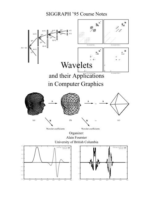
These are the notes for the Course #26, Wavelets and their Applications in Computer Graphics given at
the Siggraph ’95 Conference. They are an longer and we hope improved version of the notes for a similar
course given at Siggraph ’94 (in Orlando). The lecturers and authors of the notes are (in alphabetical order)
Michael Cohen, Tony DeRose, Alain Fournier, Michael Lounsbery, Leena-Maija Reissell, Peter Schröder
and Wim Sweldens.
Michael Cohen is on the research staff at Microsoft Research in Redmond, Washington. Until recently,
he was on the faculty at Princeton University. He is one of the originators of the radiosity method for
image synthesis. More recently, he has been developing wavelet methods to create efficient algorithms for
geometric design and hierarchical spacetime control for linked figure animation.
Tony DeRose is Associate Professor at the Department of Computer Science at the University of Washington.
His main research interests are computer aided design of curves and surfaces, and he has applied wavelet
techniques in particular to multiresolution representation of surfaces.
Alain Fournier is a Professor in the Department of Computer Science at the University of British Columbia.
His research interests include modelling of natural phenomena, filtering and illumination models. His
interest in wavelets derived from their use to represent light flux and to compute local illumination within a
global illumination algorithm he is currently developing.
Michael Lounsbery is currently at Alias Research in Seattle (or the company formerly known as such). He
obtained his PhD from the University of Washington with a thesis on multi-resolution analysis with wavelet
bases.
Leena Reissell is a Research Associate in Computer Science at UBC. She has developed wavelet methods
for curves and surfaces, as well as wavelet based motion planning algorithms. Her current research interests
include wavelet applications in geometric modeling, robotics, and motion extraction.
Peter Schröder received his PhD in Computer Science from Princeton University where his research focused
on wavelet methods for illumination computations. He continued his work with wavelets as a Postdoctoral
Fellow at the University of South Carolina where he has pursued generalizations of wavelet constructions.
Other research activities of his have included dynamic modelling for computer animation, massively parallel
graphics algorithms, and scientific visualization.
Wim Sweldens is a Research Assistant of the Belgian National Science Foundation at the Department of

2 A. FOURNIER
Computer Science of the Katholieke Universiteit Leuven, and a Research Fellow at the Department of
Mathematics of the University of South Carolina. He just joined the applied mathematics group at ATT Bell
Laboratories. His research interests include the construction of non-algebraic wavelets and their applications
in numerical analysis and image processing. He is one of the most regular editors of the Wavelet Digest.
In the past few years wavelets have been developed both as a new analytic tool in mathematics and as a
powerful source of practical tools for many applications from differential equations to image processing.
Wavelets and wavelet transforms are important to researchers and practitioners in computer graphics because
they are a natural step from classic Fourier techniques in image processing, filtering and reconstruction, but
also because they hold promises in shape and light modelling as well. It is clear that wavelets and wavelet
transforms can become as important and ubiquitous in computer graphics as spline-based technique are now.
This course, in its second instantiation, is intented to give the necessary mathematical background on
wavelets, and explore the main applications, both current and potential, to computer graphics. The emphasis
is put on the connection between wavelets and the tools and concepts which should be familiar to any skilled
computer graphics person: Fourier techniques, pyramidal schemes, spline representations. We also tried to
give a representative sample of recent research results, most of them presented by their authors.
The main objective of the course (through the lectures and through these notes) is to provide enough
background on wavelets so that a researcher or skilled practitioner in computer graphics can understand
the nature and properties of wavelets, and assess their suitability to solve specific problems in computer
graphics. Our goal is that after the course and/or the study of these notes one should be able to access the
basic mathematical literature on wavelets, understand and review critically the current computer graphics
literature using them, and have some intuition about the pluses and minuses of wavelets and wavelet
transform for a specific application.
We have tried to make these notes quite uniform in presentation and level, and give them a common list of
references, pagination and style. At the same time we hope you still hear distinct voices. We have not tried
to eradicate redundancy, because we believe that it is part and parcel of human communication and learning.
We tried to keep the notation consistent as well but we left variations representative of what is normally
found in the literature. It should be noted that the references are by no mean exhaustive. The literature of
wavelets is by now huge. The entries are almost exclusively references made in the text, but see Chapter
VIII for more pointers to the literature.
The CD-ROM version includes an animation (720 frames) made by compressing (see Chapter IV) and
reconstructing 6 different images (the portraits of the lecturers) with six different wavelet bases. The text
includes at the beginning of the first 6 chapters four frames (at 256 256 resolution originally) of each
sequence. This gives an idea (of course limited by the resolution and quality of the display you see them
on) of the characteristics and artefacts associated with the various transforms. In order of appearance,
the sequences are Alain Fournier with Adelson bases, Leena-Maija Reissell with pseudo-coiflets, Michael
Lounsbery with Daubechies 4, Wim Sweldens with Daubechies 8, Tony DeRose with Battle-Lemarié, Peter
Schröder with Haar and Michael Cohen with coiflets 4. All of these (with the exception of Adelson) are
described in the text. Michael Lounsbery version does not appear in the CD-ROM due to lack of time.
Besides the authors/lecturers, many people have helped put these notes together. Research collaborators
are identified in the relevant sections, some of them as co-authors. The latex/postscript version of these
notes have been produced at the Department of Computer Science at the University of British Columbia.
Last year Chris Romanzin has been instrumental in bringing them into existence. Without him they would
Siggraph ’95 Course Notes: #26 Wavelets

PREAMBLE 3
be a disparate collection of individual sections, and Alain Fournier’s notes would be in troff. This year
Christian Vinther picked up the torch, and thanks to Latex amazing memory, problems we had licked
last year reappeared immediately. That gave him a few fun nights removing most of them. Bob Lewis,
also at UBC, has contributed greatly to the content of the first section, mostly through code and general
understanding of the issues. The images heading the chapters, and the animation found on the CD-ROM
were all computed with his code (also to be found on the disc -see Chapter VIII). Parag Jain implemented an
interactive program which was useful to explore various wavelet image compressions. Finally we want to
thank Stephan R. Keith (even more so than last year) the production editor of the CD-ROM, who was most
helpful, patient and efficient as he had to deal with dozens of helpless, impatient and scattered note writers.
Alain Fournier
Siggraph ’95 Course Notes: #26 Wavelets

4 A. FOURNIER
Siggraph ’95 Course Notes: #26 Wavelets

1 Scale
1.1 Image pyramids
I: Introduction
Alain FOURNIER
University of British Columbia
Analyzing, manipulating and generating data at various scales should be a familiar concept to anybody
involved in Computer Graphics. We will start with “image” pyramids 1 .
In pyramids such as a MIP map used for filtering, successive averages are built from the initial signal.
Figure I.1 shows a schematic representation of the operations and the results.
Figure I.1: Mean pyramid
Sum
Difference
Stored value
Addition
Subtraction
It is clear that it can be seen as the result of applying box filters scaled and translated over the signal. For n
initial values we have log 2 (n) stages, and 2n,1 terms in the result. Moreover because of the order we have
1 We will use the word “image” even though our examples in this section are for 1D signals.

6 A. FOURNIER
chosen for the operations we only had to compute n , 1 additions (and shifts if means are stored instead of
sums).
This is not a good scheme for reconstruction, since all we need is the last row of values to reconstruct the
signal (of course they are sufficient since they are the initial values, but they are also necessary since only
a sum of adjacent values is available from the levels above). We can observe, though, that there is some
redundancy in the data. Calling si;j the jth element of level i (0 being the top of the pyramid, k = log 2 (n)
being the bottom level) we have:
si;j = (si+1;2j + si+1;2j+1)
2
We can instead store s0;0 as before, but at the level below we store:
s 0 1;0 = (s1;0 , s1;1)
2
It is clear that by adding s0;0 and s 0 1;0 we retrieve s1;0 andbysubtractings0;0 and s 0 1;0
we retrieve s1;1.
We therefore have the same information with one less element. The same modification applied recursively
through the pyramid results in n , 1 values being stored in k , 1 levels. Since we need the top value as
well (s0;0), and the sums as intermediary results, the computational scheme becomes as shown in Figure I.2.
The price we have to pay is that now to effect a reconstruction we have to start at the top of the pyramid and
stop at the level desired. The computational scheme for the reconstruction is given in Figure I.3.
Figure I.2: Building the pyramid with differences
Sum
Difference
Stored value
Sum
Addition
Subtraction
Difference
Stored value
Figure I.3: Reconstructing the signal from difference pyramid
Siggraph ’95 Course Notes: #26 Wavelets
Addition
Subtraction

INTRODUCTION 7
If we look at the operations as applying a filter to the signal, we can see easily that the successive filters
in the difference pyramid are (1/2, 1/2) and (1/2, -1/2), their scales and translates. We will see that they
are characteristics of the Haar transform. Notice also that this scheme computes the pyramid in O(n)
operations.
2 Frequency
The standard Fourier transform is especially useful for stationary signals, that is for signals whose properties
do not change much (stationarity can be defined more precisely for stochastic processes, but a vague concept
is sufficient here) with time (or through space for images). For signals such as images with sharp edges
and other discontinuities, however, one problem with Fourier transform and Fourier synthesis is that in
order to accommodate a discontinuity high frequency terms appear and they are not localized, but are added
everywhere. In the following examples we will use for simplicity and clarity piece-wise constant signals and
piece-wise constant basis functions to show the characteristics of several transforms and encoding schemes.
Two sample 1-D signals will be used, one with a single step, the other with a (small) range of scales in
constant spans. The signals are shown in Figure I.4 and Figure I.5.
10
8
6
4
2
0
12
10
8
6
4
2
0
0 5 10 15 20 25 30
Figure I.4: Piece-wise constant 1-D signal (signal 1)
0 5 10 15 20 25 30
Figure I.5: Piece-wise constant 1-D signal (signal 2)
Siggraph ’95 Course Notes: #26 Wavelets

8 A. FOURNIER
3 The Walsh transform
A transform similar in properties to the Fourier transform, but with piece-wise constant bases is the Walsh
transform. The first 8 basis functions of the Walsh transform Wi(t) are as shown in Figure I.6. The Walsh
Walsh 0
Walsh 1
Walsh 2
Walsh 3
Walsh 4
Walsh 5
Walsh 6
Walsh 7
0 2 4 6 8 10 12 14 16
functions are normally defined for , 1 1
2 t 2
Figure I.6: First 8 Walsh bases
, and are always 0 outside of this interval (so what is plotted
in the preceding figure is actually Wi( t
16 , 1 2 )). They have various ordering for their index i, soalways
make sure you know which ordering is used when dealing with Wi(t). The most common, used here, is
where i is equal to the number of zero crossings of the function (the so-called sequency order). They are
various definitions for them (see [14]). A simple recursive one is:
W2j+q(t) =(,1) j
2 +q
[ Wj (2t + 1
2 )+(,1)(j+q) Wj (2t , 1
2 )]
with W0(t) =1. Where j ranges from 0 to1 and q = 0 or 1. The Walsh transform is a series of coefficients
given by:
wi =
Z 1
2
, 1
2
f (t) Wi(t) dt
Siggraph ’95 Course Notes: #26 Wavelets

and the function can be reconstructed as:
f (t) =
1X
i=0
wi Wi(t)
Figures I.7 and I.8 show the coefficients of the Walsh basis for both of the above signals.
5
4
3
2
1
0
-1
-1
-2
-3
0123456
INTRODUCTION 9
0 5 10 15 20 25 30
Figure I.7: Walsh coefficients for signal 1.
0 5 10 15 20 25 30
Figure I.8: Walsh coefficients for signal 2.
Note that since the original signals have discontinuities only at integral values, the signals are exactly
represented by the first 32 Walsh bases at most. But we should also note that in this example, as well as
would be the case for a Fourier transform, the presence of a single discontinuity at 21 for signal 1 introduces
the highest “frequency” basis, and it has to be added globally for all t. In general cases the coefficients for
each basis function decrease rapidly as the order increases, and that usually allows for a simplification (or
compression) of the representation of the original signal by dropping the basis functions whose coefficients
are small (obviously with loss of information if the coefficients are not 0).
Siggraph ’95 Course Notes: #26 Wavelets

10 A. FOURNIER
4 Windowed Fourier transforms
One way to localize the high frequencies while preserving the linearity of the operator is to use a windowed
Fourier transform (WFT ) also known as a short-time Fourier transform (STFT ). Given a window function
w(t) (we require that the function has a finite integral and is non-zero over a finite interval) we define the
windowed Fourier transform of the signal f (t) as:
FW ( ;f)=
Z 1
,1
f (t) w (t , ) e ,2i ft dt
In words, the transform is the Fourier transform of the signal with the filter applied. Of course we got a
two-variable function as an answer, with , the position at which the filter is applied, being the additional
variable. This was first presented by Gabor [87]. It is clear that the filter function w(t) allows us a window on
the frequency spectrum of f (t) around . An alternate view is to see the filter impulse response modulated
to the frequency being applied to the Fourier transform of the signal f (t) “for all times” (this is known in
signal processing as a modulated filter bank).
We have acquired the ability to localize the frequencies, but we have also acquired some new problems.
One, inherent to the technique, is the fact we have one more variable. Another is that it is not possible to get
high accuracy in both the position (in time) and frequency of a contributing discontinuity. The bandwidth,
or spread in frequency, of the window w(t), with W (f ) its Fourier transform, can be defined as:
The spread in time is given by:
Δf 2 =
Δt 2 =
R f 2 jW (f )j 2 df
R jW (f )j 2 df
R t 2 jw(t)j 2 dt
R jw(t)j 2 dt
By Parseval’s theorem both denominators are equal, and equal to the energy of w(t). In both cases these
values represent the root mean square average (other kinds of averages could be considered).
Exercise 1: Compute Δf and Δt for the box filter as a function of A and T0. 2
If we have a signal consisting of two pulses in time, they cannot be discriminated by a WFT using this w(t)
if they are Δt apart or less. Similarly two pure sine waves ( pulses in frequency) cannot be discriminated if
they are Δf apart or less. We can improve the frequency discrimination by choosing a w(t) with a smaller
Δf, and similarly for time, but unfortunately they are not independent. In fact there is an equality, the
Siggraph ’95 Course Notes: #26 Wavelets

Heisenberg inequality that bounds their product:
Δt Δf
1
4
INTRODUCTION 11
The lower bound is achieved by the Gaussian [87]. The other aspect of this problem is that once the window
is chosen, the resolution limit is the same over all times and frequencies. This means that there is no
adaptability of the analysis, and if we want good time resolution of the short bursts, we have to sacrifice
good frequency description of the long smooth sections.
To illustrate with a piece-wise constant transform, we can use the Walsh transform again, and use a box as
the window. The box is defined as:
(
1
w(t) =
0
if , 2 t

12 A. FOURNIER
5 Relative Frequency Analysis
One obvious “fix” to this problem is to let the window, and therefore the Δf vary as a function of the
frequency. A simple relation is to require Δf
f
= c, c being a constant. This approach is been used in signal
processing, where it is known as constant-Q analysis. Figure I.11 illustrates the difference in frequency
space between a constant bandwidth window and a constant relative bandwidth window (there c = 2).
The goal is to increase the resolution in time (space) for sharp discontinuitieswhile keeping a good frequency
resolution at high frequencies. Of course if the signal is composed of high frequencies of long duration (as
in a very noisy signal), this strategy does not pay off, but if the signal is composed of relatively long smooth
areas separated by well-localized sharp discontinuities (as in many real or computer-generated images and
scenes) then this approach will be effective.
6 Continuous Wavelet Transform
We can choose any set of windows to achieve the constant relative bandwidth, but a simple version is if all
the windows are scaled version of each other. To simplify notation, let us define h(t) as:
and scaled versions of h(t):
,2i f0t
h(t) =w(t) e
ha(t) = 1
p h(
jaj t
a )
where a is the scale factor (that is f = f0
a ), and the constant 1
now becomes:
WF ( ;a)= 1
p
jaj
p jaj is for energy normalization. The WFT
Z f (t) h ( t , a ) dt
This is known as a wavelet transform, andh(t) is the basic wavelet. It is clear from the above formula
that the basic wavelet is scaled, translated and convolved with the signal to compute the transform. The
translation corresponds to moving the window over the time signal, and the scaling, which is often called
dilation in the context of wavelets, corresponds to the filter frequency bandwidth scaling.
We have used the particular form of h(t) related to the window w(t), but the transform WF () can be
defined with any function h(t) satisfying the requirements for a bandpass function, that is it is sufficiently
regular (see [162] for a definition of regular) its square integral is finite (in the L 2 sense) and its integral
R h(t) dt = 0.
We can rewrite the basic wavelet as:
ha; = 1 p h(
a t , a )
to emphasize that we use a set of “basis” functions. The transform is then written as:
WF ( ;a)=
Z f (t) ha; (t) dt
Siggraph ’95 Course Notes: #26 Wavelets

We can reconstruct the signal as:
Z
da dt
f (t) =c WF ( ;a) ha; (t)
a2 INTRODUCTION 13
where c is a constant depending on h(t). The reconstruction looks like a sum of coefficients of orthogonal
bases, but the ha; (t) are in fact highly redundant, since they are defined for every point in the a; space.
Nevertheless the formula above is correct if R h 2 (t) dt is finite and R h(t) dt = 0 (well, almost).
7 From Continuous to Discrete and Back
Since there is a lot of redundancy in the continuous application of the basic wavelet, a natural question
if whether we can discretize a and in such a way that we obtain a true orthonormal basis. Following
Daubechies [49] one can notice that if we consider two scales a0

14 A. FOURNIER
a new set of basis functions (of course it remains to be proved that they are really basis functions). These
happen to be the Haar functions, defined by Haar [99] and well known today as the bases for piece-wise
constant wavelets (see Figure I.14).
Figures I.15 and I.16 show the coefficients of the Haar basis for both of our exemplar signals. Figure
I.17 shows the Haar coefficients for signal 2 with circles for easier comparisons with the windowed Walsh
transform.
One can prove that the same information is contained in these 32 values that was in the 31 32 values of
the windowed Walsh transforms. It is also clear from the plots that there are many zero coefficients, and in
particular for signal 1 the magnitude of the Haar coefficients localize the discontinuities in the signal.
7.2 Image Pyramids Revisited
We can now generalize the concept of image pyramids to what is known in filtering as a subband coding
scheme. We have applied recursively two operators to the signal to subsample it by 2. The first one is
the box, and is a smoothing, oralow-pass filter, and the other is the basic Haar wavelet, or a detail or a
high-pass filter. In our specific example the detail filter picks out exactly what is necessary to reconstruct
the signal later. In general, if we have a low-pass filter h(n), a high-pass filter g(n), and a signal f (n) 3 ,we
can compute the subsampled smooth version:
and the subsampled detail version:
a(k) =
d(k) =
X
i
X
i
f (i) h(,i + 2k)
f (i) g(,i + 2k)
If the smoothing filter is orthogonal to its translates, then the two filters are related as:
g(L, 1 , i) =(,1) i h(i)
(where L is the length of the filter, which is assumed finite and even). The reconstruction is then exact, and
computed as:
f (i) =
X
k
[ a(k) h(,i + 2k) +d(k) g(,i + 2k)]
We can apply this scheme recursively to the new smoothed signal a(), which is half the size of f (), until we
have two vectors a() and d() of length 1 after log 2 (n) applications. It is clear that as in the Haar transform
this scheme has only O(n) cost. The computational scheme is shown in Figure I.18. The computational
scheme for the reconstruction is given in Figure I.19. H is the application (sum over i) of the smoothing
filter, G the application of the detail filter, and H and G denote the sum over k of the smoothing and detail
filters, respectively.
3 It would be better to call l() the low pass filter and h() the high pass filter, and some do, but we will use here the usual symbols.
Siggraph ’95 Course Notes: #26 Wavelets

7.3 Dyadic Wavelet Transforms
INTRODUCTION 15
We have sort of “stumbled” upon the Haar wavelet, from two different directions (from the windowed Walsh
transform and from the difference pyramid). We need better methods than that to construct new wavelets
and express their basic properties. This is exactly what most of the recent work on wavelets is about [50].
We reproduce the following development from Mallat & Zhong [133]. Consider a wavelet function (t).
All we ask is that its average R (t) dt = 0. Let us write i(t) its dilation by a factor of 2 i :
i = 1 t
(
2i 2
The wavelet transform of f (t) at scale 2 i is given by:
WFi(t) = f i(t) =
Z 1
The dyadic wavelet transform is the sequence of functions
,1
i )
f ( ) i(t , ) d
WF[f ()] = [WFi(t)] i 2 Z
We want to see how well WF represents f (t) and how to reconstruct it from its transform. Looking at the
Fourier transform (we use F (f ) or F[f (t)] as notation for the Fourier transform of f (t)):
F[WFi(t)] = F (f ) Ψ(2 i f ) (1)
If we impose that there exists two strictly positive constants A and B such that:
8f; A
1X
jΨ(2
i=,1
if )j2 B (2)
we guarantee that everywhere on the frequency axis the sum of the dilations of () have a finite norm.
If this is true, then F (f ), and therefore f (t) can be recovered from its dyadic wavelet transform. The
reconstructing wavelet (t) is any function such that its Fourier transform X(f ) satisfies:
1X
i=,1
Ψ(2 i f ) X(2 i f )=1 (3)
An infinity of () satisfies (3) if (2) is valid. We can then reconstruct f (t) using:
f (t) =
1X
WFi(t) i(t) (4)
i=,1
Siggraph ’95 Course Notes: #26 Wavelets

16 A. FOURNIER
Exercise 2: Prove equation (4) by taking its Fourier transform, and inserting (1) and (3). 2
Using Parseval’s theorem and equations (2) and (4), we can deduce a relation between the norms of f (t)
and of its wavelet transform:
A k f ()k 2
1X
k WFi(t)k
i=,1
2
B k f ()k 2
This proves that the wavelet transform is also stable, and can be made close in the L 2 norm by having A
B
close to 1.
It is important to note that the wavelet transform may be redundant, in the sense that the some of the
information in Wi can be contained in others Wj subspaces. For a more precise statement see [133]
7.4 Discrete Wavelet Transform
To obtain a discrete transform, we have to realize that the scales have a lower limit for a discrete signal. Let
us say that i = 0 correspond to the limit. We introduce a new smoothing function () such that its Fourier
transform is:
From (3) one can prove that R
now define the operator:
with i(t) = 1
2 i
j Φ(f )j 2 =
1X
i=1
(5)
Ψ(2 i f ) X(2 i f ) (6)
(t) dt = 1, and therefore is really a smoothing function (a filter). We can
Z
SFi(t) = f ( ) i(t , ) d
( t
2 i ). SoSFi(t) is a smoothing of f (t) at scale 2 i . From equation (6) we can write:
j Φ(f )j 2 ,jΦ(2 j )j 2 =
jX
i=1
Ψ(2 i f ) X(2 i f )
This shows that the high frequencies of f (t) removed by the smoothing operation at scale 2 j can be recovered
by the dyadic wavelet transform WFi(t),1 i j.
Now we can handle a discrete signal fn by assuming that there exists a function f (t) such that:
SF1(n) = fn
This function is not necessarily unique. We can then apply the dyadic wavelet transforms of f (t) at the
larger scales, which need only the values of f (n + w),wherew are integer shifts depending on () and the
scale. Then the sequence of SFi(n) and WFi(n) is the discrete dyadic wavelet transform of fn. Thisisof
course the same scheme used in the generalized multiresolution pyramid. This again tells us that there is a
O(n) scheme to compute this transform.
Siggraph ’95 Course Notes: #26 Wavelets

7.5 Multiresolution Analysis
INTRODUCTION 17
A theoretical framework for wavelet decomposition [130] can be summarized as follows. Given functions
in L 2 (this applies as well to vectors) assume a sequence of nested subspaces Vi such that:
V,2 V,1 V0 V1 V2
If a function f (t) 2 Vi then all translates by multiples of 2 ,i also belongs (f (t , 2 ,i k) 2 Vi). We also
want that f (2t) 2 Vi+1. If we call Wi the orthogonal complement of Vi with respect to Vi+1. We write it:
Vi+1 = Wi Vi
In words, Wi has the details missing from Vi to go to Vi+1. By iteration, any space can be reached by:
Vi = Wi Wi,1 Wi,2 Wi,3 (7)
Therefore every function in L 2 can be expressed as the sum of the spaces Wi. IfV0 admits an orthonormal
basis j(t , j) and its integer translates (2 0 = 1), then Vi has ij = cj (2 i , j) as bases. There will exist
a wavelet 0() which spans the space W0 with its translates, and its dilations ij() will span Wi. Because
of (7), therefore, every function in L 2 can be expressed as a sum of ij(),awavelet basis. We then see that
a function can be expressed as a sum of wavelets, each representing details of the function at finer and finer
scales.
A simple example of a function is a box of width 1. If we take as V0 the space of all functions constant
within each integer interval [ j; j + 1 ), it is clear that the integer translates of the box spans that space.
Exercise 3: Show that boxes of width 2 i span the spaces Vi. Should there be a scaling factor when
going from width 2 i to 2 i,1 . Show that the Haar wavelets are the basis for Wi corresponding to the box for
Vi. 2
7.6 Constructing Wavelets
7.6.1 Smoothing Functions
To develop new dyadic wavelets, we need to find smoothing functions () which obey the basic dilation
equation:
(t) =
X
k
ck (2t , k)
Siggraph ’95 Course Notes: #26 Wavelets

18 A. FOURNIER
This way, each i can be expressed as a linear combination of its scaled version, and if it cover the subspace
V0 with its translates, its dyadic scales will cover the other Vi subspace. Recalling that R
(t) dt = 1, and
integrating both sides of the above equation, we get:
Z
(t) dt =
X
k
ck
Z
(2t , k) dt
and since d(2t , k) =2dt, then P k ck = 2. One can see that when c0 = c1 = 1, for instance, we obtain
the box function, which is the Haar smoothing function.
Three construction methods have been used to produce new (t) (see Strang [177] for details).
1. Iterate the recursive relation starting with the box function and some c values. This will give the
splines family (box, hat , quadratic, cubic, etc..) with the initial values [1,1], [ 1 1 1 3 3
; 1; ], [ ; ;
1
2 2 4 4 4 ; 4 ],
[ 1 8 ; 4 8 ; 6 8 ; 4 8 ; 1 8 ]. One of Daubechies’ wavelets, noted D4, is obtained by this method with
[ 1+
p
3
4 ; 3+
p
3
4 ; 3,p3 4 ; 1,p3 4 ].
2. Work from the Fourier transform of () (equation (6)). Imposing particular forms on it and the Fourier
transform of () and () can lead to a choice of suitable functions. See for instance in Mallat &
Zhong [133] how they obtain a wavelet which is the derivative of a cubic spline filter function.
3. Work directly with the recursion. If () is known at the integers, applying the recursion gives the
values at all points of values i
2 j .
7.6.2 Approximation and Orthogonality
The basic properties for approximation accuracy and orthogonality are given, for instance, in Strang [177].
The essential statement is that a number p characterize the smoothing function () such that:
– polynomials of degree p , 1 are linear combinations of () and its translates
– smooth functions are approximated with error O(h p ) at scale h = 2 ,j
– thefirstp moments of () are 0:
Z t n (t) dt = 0; n = 0;:::;p, 1
Those are known as the vanishing moments. For Haar, p = 1, for D4 p = 2.
The function () is defined as (), but using the differences:
X k
(t) = (,1) c1,k (2t , k)
The function so defined is orthogonal to () and its translates. If the coefficients ci are such that
X ckck,2m = 2 0m
and 0() is orthogonal to its translates, then so are all the i() at any scale, and the i() at any scale. If they
are constructed from the box function as in method 1, then the orthogonality is achieved.
Siggraph ’95 Course Notes: #26 Wavelets

7.7 Matrix Notation
INTRODUCTION 19
A compact and easy to manipulate notation to compute the transformations is using matrices (infinite in
principle). Assuming that ci;i = 0 :::L, 1 are the coefficients of the dilation equation then the matrix
[H] is defined such that Hij = 1
2 c2i,j. The matrix [G] is defined by Gij = 1
2 (,1)j+1 cj+1,2i. The factor
1
1
2 could be replaced by p for energy normalization (note that sometimes this factor is already folded into
2
the ci, be sure you take this into account for coding). The matrix [H] is the smoothing filter (the restriction
operator in multigrid language), and [G] the detail filter (the interpolation operator).
The low-pass filtering operation is now applying the [H] matrix to the vector of values f. The size of the
submatrix applied is n
2 n if n is the original size of the vector 2J = n. The length of the result is half
the length of the original vector. For the high pass filter the matrix [G] is applied similarly. The process is
repeated J times until only one value each of a and d is obtained.
The reconstruction matrices in the orthogonal cases are merely the transpose of [H ]=[H] T and [G ]=
1 is used, p otherwise). The reconstruction operation is then:
2
[G] T (with factor of 1 if 1
2
with j = 1;:::;J. as shown in Figure I.19.
a j =[H ] a j,1 +[G ] d j,1
As an example we can now compute the wavelet itself, by inputing a unit vector and applying the inverse
wavelet transform. For example, the fifth basis from D4 is given in Figure I.20.
Of course by construction all the other bases are translated and scaled versions of this one.
7.8 Multiscale Edge Detection
There is an important connection between wavelets and edge detection, since wavelets transforms are well
adapted to “react” locally to rapid changes in values of the signal. This is made more precise by Mallat and
Zhong [133]. Given a smoothing function () (related to (), but not the same), such that R (t) dt = 1and
it converges to 0 at infinity, if its first and second derivative exist, they are wavelets:
1 (t) =
d (t)
dt
and 2 (t) = d2 (t)
dt 2
If we use these wavelets to compute the wavelet transform of some function f (t), noting a(t) = 1
a
WF 1 a(t) = f 1 a (t) =f (ad a d
)(t) =a
dt dt (f a)(t)
WF 2 a(t) = f 2 a (t) = f (a2 d2 a
d2
)(t) =a2
dt2 dt2 (f a)(t)
So the wavelet transforms are the first and second derivative of the signal smoothed at scale a. The local
extrema of WF 1 a(t) are zero-crossings of WF 2 a(t) and inflection points of f a(t). If (t) is a Gaussian,
then zero-crossing detection is equivalent to the Marr-Hildreth [139] edge detector, and extrema detection
equivalent to Canny [17] edge detection.
Siggraph ’95 Course Notes: #26 Wavelets
( t
a ):

20 A. FOURNIER
8 Multi-dimensional Wavelets
For many applications, in particular for image processing and image compression, we need to generalize
wavelets transforms to two dimensions. First, we will consider how to perform a wavelet transform of
the pixel values in a two-dimensional image. Then the scaling functions and wavelets that form a twodimensional
wavelet basis. We will use the Haar basis as a simple example, but it will apply to other
basesaswell 4 . There are two ways we can generalize the one-dimensional wavelet transform to two
dimensions, standard and non-standard decomposition (since a multi-dimensional wavelet transform is
frequently referred to in the literature as a wavelet decomposition, we will use that term in this section).
8.1 Standard Decomposition
To obtain the standard decomposition [15] of an image, we first apply the one-dimensional wavelet transform
to each row of pixel values. This operation gives us an average value along with detail coefficients for
each row. Next, we treat these transformed rows as if they were themselves an image, and apply the
one-dimensional transform to each column. The resulting values are all detail coefficients except for a
single overall average coefficient. We illustrate each step of the standard decomposition in Figure I.21.
The standard decomposition of an image gives coefficients for a basis formed by the standard construction
[15] of a two-dimensional basis. Similarly, the non-standard decomposition gives coefficients for the
non-standard construction of basis functions.
The standard construction of a two-dimensional wavelet basis consists of all possible tensor products of
one-dimensional basis functions. For example, when we start with the one-dimensional Haar basis for V 2 ,
we get the two-dimensional basis for V 2 that is shown in Figure I.22. In general we define the new functions
from the 1D smooth and wavelet functions:
(u) (v) (u) (v) (u) (v) (u) (v)
These are orthogonal if the 1-D version are, and the first is a smoothing function, the other three are wavelets.
8.2 Non-Standard Decomposition
The second type of two-dimensional wavelet transform, called the non-standard decomposition, alternates
between operations on rows and columns. First, we perform one step of horizontal pairwise averaging
and differencing on the pixel values in each row of the image. Next, we apply vertical pairwise averaging
and differencing to each column of the result. To complete the transformation, we repeat this process
recursively on the quadrant containing averages in both directions. Figure I.23 shows all the steps involved
in the non-standard decomposition of an image.
The non-standard construction of a two-dimensional basis proceeds by first defining a two-dimensional
scaling function,
(x; y) := (x) (y);
4
This section is largely copied, with kind permission, from a University of Washington Technical Report (94-09-11) by Eric
Stollnitz, Tony DeRose and David Salesin.
Siggraph ’95 Course Notes: #26 Wavelets

and three wavelet functions,
(x; y) := (x) (y)
(x; y) := (x) (y)
(x; y) := (x) (y):
INTRODUCTION 21
The basis consists of a single coarse scaling function along with all possible scales and translates of the
three wavelet functions. This construction results in the basis for V 2 shown in Figure I.24.
We have presented both the standard and non-standard approaches to wavelet transforms and basis functions
because they each have advantages. The standard decomposition of an image is appealing because it can
be accomplished simply by performing one-dimensional transforms on all the rows and then on all the
columns. On the other hand, it is slightly more efficient to compute the non-standard decomposition of
an image. Each step of the non-standard decomposition computes one quarter of the coefficients that the
previous step did, as opposed to one half in the standard case.
Another consideration is the support of each basis function, meaning the portion of each function’s domain
where that function is non-zero. All of the non-standard basis functions have square supports, while some
of the standard basis functions have non-square supports. Depending upon the application, one of these
choices may be more favorable than another.
8.3 Quincunx Scheme
One can define a sublattice in Z 2 by selecting only points (i; j) which satisfies:
i
j
!
=
1 1
1 ,1
! m
n
for all m; n 2 Z. One can construct non-separable smoothing and detail functions based on this sampling
matrix, with a subsampling factor of 2 (as opposed to 4 in the separable case). The iteration scheme is then
identical to the one for the 1-D case [50].
9 Applications of Wavelets in Graphics
Except for the illustration of signal compression in 1D, this is only a brief overview. The following sections
cover most of these topics in useful details.
9.1 Signal Compression
A transform can be used for signal compression, either by keeping all the coefficients, and hoping that there
will be enough 0 coefficients to save space in storage (and transmission). This will be a loss-less compression,
and clearly the compression ratio will depend on the signal. Transforms for our test signals indicate that
there are indeed many 0 coefficients for simple signals. If we are willing to lose some information on the
signal, we can clamp the coefficients, that is set to 0 all the coefficients whose absolute values are less than
some threshold (user-defined). One can then reconstruct an approximation (a “simplified” version) of the
original signal. There is an abundant literature on the topic, and this is one of the biggest applications of
Siggraph ’95 Course Notes: #26 Wavelets
!

22 A. FOURNIER
wavelets so far. Chapter IV covers this topic.
To illustrate some of the results with wavelets vs we can test the transforms on signals more realistic than
our previous examples (albeit still 1D).
The following figure (Figure I.25) shows a signal (signal 3) which is made of 256 samples of the red signal
off a digitized video frame of a real scene (a corner of a typical lab). Figure I.26 shows the coefficients
of the Walsh transform for this signal. If we apply the Haar transform to our exemplar signal, we obtain
the following coefficients (Figure I.27). We can now reconstruct that signal, but first we remove all the
coefficients whose absolute value is not greater than 1 (which leaves 28 non-zero coefficients). The result is
shown in Figure I.28. For another example we use one of Daubechies’ wavelets, noted D4. It is a compact
wavelet, but not smooth. We obtain the following coefficients (Figure I.29).
We can now reconstruct that signal, this time clamping the coefficients at 7 (warning: this is sensitive to the
constants used in the transform). This leaves 35 non-zero coefficients. The result is shown in Figure I.30.
Siggraph ’95 Course Notes: #26 Wavelets

0.0
0.0
Figure I.10: Signal 2 analysed with windowed Walsh transform
INTRODUCTION 23
0 2 4 6 8 10 12
Figure I.11: Constant bandwidth vs constant relative bandwidth window
Siggraph ’95 Course Notes: #26 Wavelets

24 A. FOURNIER
6
5
4
3
2
1
0
-1
-2
Figure I.12: Signal 2 analysed with scaled windowed Walsh transform
-3
0 100 200 300 400 500 600 700 800 900 1000
Figure I.13: Signal 2 analysed with scaled windowed Walsh transform (bar graph)
Siggraph ’95 Course Notes: #26 Wavelets

Haar 0
Haar 1
Haar 2
Haar 3
Haar 4
Haar 5
Haar 6
Haar 7
INTRODUCTION 25
0 2 4 6 8 10 12 14 16
Figure I.14: First 8 Haar bases
Siggraph ’95 Course Notes: #26 Wavelets

26 A. FOURNIER
4.5 5
3.5 4
2.5 3
1.5 2
0.5
0
1
6
5
4
3
2
1
0
-1
-2
0 5 10 15 20 25 30
Figure I.15: Haar coefficients for signal 1.
0 5 10 15 20 25 30
Figure I.16: Haar coefficients for signal 2.
Figure I.17: Haar coefficients for signal 2 (circle plot).
Siggraph ’95 Course Notes: #26 Wavelets

f[n] = a[n]
f[n] = a[n]
H
G
a[n/2]
d[n/2]
G
H
a[n/4] a[n/8] a[1]
d[n/4]
G
H
d[n/8]
Figure I.18: Discrete wavelet transform as a pyramid
H*
G*
a[n/2]
d[n/2]
H*
G*
H
G
INTRODUCTION 27
d[1]
a[n/4] a[n/8] a[1]
d[n/4]
H*
G*
d[n/8]
H*
G*
Figure I.19: Reconstructing the signal from wavelet pyramid
Siggraph ’95 Course Notes: #26 Wavelets
d[1]

28 A. FOURNIER
2
1.5
1
0.5
0
-0.5
-1
-1.5
Figure I.20: Wavelet basis function (from D4)
transform rows
-
transform
columns
?
Figure I.21: Standard decomposition of an image.
Siggraph ’95 Course Notes: #26 Wavelets
.

0
0 (x) 1 1 (y)
0
0 (x) 1 0 (y)
0
0 (x) 0 0 (y)
0
0 (x) 0 0 (y)
0 0 (x) 1 1 (y)
0 0 (x) 1 0 (y)
0 0 (x) 0 0 (y)
0 0 (x) 0 0 (y)
1 0 (x) 1 1 (y)
1 0 (x) 1 0 (y)
1 0 (x) 0 0 (y)
1 0 (x) 0 0 (y)
1 1 (x) 1 1 (y)
1 1 (x) 1 0 (y)
1 1 (x) 0 0 (y)
1 1 (x) 0 0 (y)
INTRODUCTION 29
Figure I.22: The standard construction of a two-dimensional Haar wavelet basis for V 2 . In the unnormalized case,
functions are +1 where plus signs appear, ,1 where minus signs appear, and 0 in gray regions.
transform rows
-
?
. ..
transform
columns
Figure I.23: Non-standard decomposition of an image.
Siggraph ’95 Course Notes: #26 Wavelets

30 A. FOURNIER
1
0 (x) 1 1 (y)
1
0 (x) 1 0 (y)
0
0 (x) 0 0 (y)
0
0 (x) 0 0 (y)
1
1 (x) 1 1 (y)
1
1 (x) 1 0 (y)
0 0 (x) 0 0 (y)
0 0 (x) 0 0 (y)
1 0 (x) 1 1 (y)
1 0 (x) 1 0 (y)
1 0 (x) 1 1 (y)
1 0 (x) 1 0 (y)
1 1 (x) 1 1 (y)
1 1 (x) 1 0 (y)
1 1 (x) 1 1 (y)
1 1 (x) 1 0 (y)
Figure I.24: The non-standard construction of a two-dimensional Haar wavelet basis for V 2 .
200
180
160
140
120
100
80
60
40
20
0 50 100 150 200 250 300
30
25
20
15
10
5
0
-5
-10
-15
-20
Figure I.25: 1D section of digitized video (signal 3)
0 50 100 150 200 250
Figure I.26: Walsh transform of signal 3
Siggraph ’95 Course Notes: #26 Wavelets

30
25
20
15
10
5
0
-5
-10
-15
-20
200
180
160
140
120
100
80
60
40
INTRODUCTION 31
0 50 100 150 200 250
Figure I.27: Haar transform of signal 3
20
0 50 100 150 200 250 300
Figure I.28: Reconstructed signal 3 with 28 Haar coefficients
Siggraph ’95 Course Notes: #26 Wavelets

32 A. FOURNIER
30
25
20
15
10
5
0
-5
-10
-15
-20
200
180
160
140
120
100
80
60
40
0 50 100 150 200 250
Figure I.29: D4 transform of signal 3
20
0 50 100 150 200 250 300
Figure I.30: Reconstructed signal 3 with 35 D4 coefficients
Siggraph ’95 Course Notes: #26 Wavelets

INTRODUCTION 33
We now go through the same series with a signal (signal 4) sampled across a computer generated image
(Figure I.31). Figure I.32 shows the coefficients of the Walsh transform for this signal. If we apply the Haar
transform to this signal, we obtain the following coefficients (Figure I.33). We can now again reconstruct
the signal, but first we remove all the coefficients whose absolute value is not greater than 1 (which leaves
47 non-zero coefficients). The result is shown in Figure I.34. Now with D4. We obtain the following
coefficients (Figure I.35). Again we clamp the coefficients at 7. This leaves 70 non-zero coefficients. The
result is shown in Figure I.36.
Chapter IV will cover the topic in its practical context, image processing.
9.2 Modelling of Curves and Surfaces
This application is also only beginning, even though the concept of multi-resolution modelling has been
around, both in graphics [83] and in vision [145]. Chapter V will describe several applications in this area.
9.3 Radiosity Computations
To compute global illumination in a scene, the current favourite approach is using “radiosity” [39]. This
approach leads to a system of integral equations, which can be solved by restricting the solutions to a
subspace spanned by a finite basis. We then can choose wavelets basis to span that subspace, hoping that
the resulting matrix necessary to solve the system will be sparse. Chapter VI will elaborate on this topic.
10 Other Applications
There are many more applications of wavelets relevant to computer graphics. As a sample, Chapter VII
will survey applications to spacetime control, variational modeling, solutions of integral and differential
equations, light flux representations and computation of fractal processes.
An interesting area of application of wavelet techniques not covered here is in paint systems. A paper at this
conference (by D. F. Berman. J. T. Bartell and D. H. Salesin) describes a system based on the Haar basis
to implement multiresolution painting. The inherent hierarchy of the wavelet transform allows the user
to paint using common painting operations such as over and erase at any level of detail needed. Another
implementation of the same concept is from Luis Velho and Ken Perlin. They use a biorthogonal spline
basis for smoothness (remember that in the straightforward case the wavelet smoothing filter serves as a
reconstruction filter when the user zooms into the “empty spaces”). A price is paid in performance (more
non-zero elements in the filters), but the parameters of the trade-off are of course changing rapidly.
Siggraph ’95 Course Notes: #26 Wavelets

34 A. FOURNIER
300
250
200
150
100
50
0
0 50 100 150 200 250 300
30
20
10
0
-10
-20
-30
-40
30
20
10
0
-10
-20
-30
-40
Figure I.31: 1D section of computer generated image (signal 4)
0 50 100 150 200 250
Figure I.32: Walsh transform of signal 4
0 50 100 150 200 250
Figure I.33: Haar transform of signal 4
Siggraph ’95 Course Notes: #26 Wavelets

300
250
200
150
100
50
-10
-20
-30
-40
INTRODUCTION 35
0
0 50 100 150 200 250 300
30
20
10
0
300
250
200
150
100
50
Figure I.34: Reconstructed signal with 47 Haar coefficients
0 50 100 150 200 250
Figure I.35: D4 transform of signal 4
0
0 50 100 150 200 250 300
Figure I.36: Reconstructed signal 4 with 70 D4 coefficients
Siggraph ’95 Course Notes: #26 Wavelets

36 L-M. REISSELL
Siggraph ’95 Course Notes: #26 Wavelets

1 Introduction
II: Multiresolution and Wavelets
Leena-Maija REISSELL
University of British Columbia
This section discusses the properties of the basic discrete wavelet transform. The concentration is on
orthonormal multiresolution wavelets, but we also briefly review common extensions, such as biorthogonal
wavelets. The fundamental ideas in the development of orthonormal multiresolution wavelet bases
generalize to many other wavelet constructions.
The orthonormal wavelet decomposition of discrete data is obtained by a pyramid filtering algorithm which
also allows exact reconstruction of the original data from the new coefficients. Finding this wavelet
decomposition is easy, and we start by giving a quick recipe for doing this. However, it is surprisingly
difficult to find suitable, preferably finite, filters for the algorithm. One objective in this chapter is to find
and characterize such filters. The other is to understand what the wavelet decomposition says about the
data, and to briefly justify its use in common applications.
In order to study the properties of the wavelet decomposition and construct suitable filters, we change our
viewpoint from pyramid filtering to spaces of functions. A discrete data sequence represents a function in a
given basis. Similarly, the wavelet decomposition of data is the representation of the function in a wavelet
basis, which is formed by the discrete dilations and translations of a suitable basic wavelet. This is analx
ogous to the control point representation of a function using underlying cardinal B-spline functions.
For simplicity, we will restrict the discussion to the 1-d case. There will be some justification of selected
results, but no formal proofs. More details can be found in the texts [50] and [26] and the review paper
[113]. A brief overview is also given in [177].
1.1 A recipe for finding wavelet coefficients
The wavelet decomposition of data is derived from 2-channel subband filtering with two filter sequences
(hk), thesmoothing or scaling filter, and(gk), thedetail, orwavelet, filter. These filters should have the
following special properties:

38 L-M. REISSELL
Filter conditions:
– P k hk
p
= 2
– gj =(,1) j h1,j
– P k gk = 0
– P k hkhk+2m = 0m; for all m
At first glance, these conditions may look slightly strange, but they in fact contain the requirements for
exact reconstruction. The wavelet filter (hk) is sometimes called the mirror filter of the filter (hk), since it
is given by the elements of the scaling filter but in backwards order, and with every other element negated.
For simplicity, we only consider filters which are finite and real.
The two-element filter (1; 1), normalized suitably, is a simple example – this filter yields the Haar pyramid
scheme. Another example which satisfies these conditions is the 4-element filter
p
1 + 3
D4 :
4 p p
3 + 3
;
2 4 p 2 ; 3 , p 3
4 p 2 ; 1 , p 3
4 p ;
2
constructed by Daubechies.
We now look more closely at where these conditions come from. Two-channel filtering of the data sequence
x =(xi) by a filter (hk) means filtering which yields two new sequences:
yi =
X
k
hkx2i+k =
X
k
hk,2ixk; zi =
In matrix form, this filtering can be expressed as follows:
X
y = Hx; z = Gx:
k
gkx2i+k =
Here the matrix H =(hk,2i)ik is a convolution matrix, with every other row dropped:
0
B
@
X
::: 0 h0 h1 h2 h3 0 0 0 ::: :::
::: ::: ::: 0 h0 h1 h2 h3 0 0 :::
::: ::: ::: ::: ::: 0 h0 h1 h2 h3 0
:::
k
gk,2ixk: (1)
The matrix G is defined similarly using the detail filter (gk). The 2-channel filtering process “downsamples”
(by dropping alternate rows from the convolution matrix) and produces a sequence half the length of the
Siggraph ’95 Course Notes: #26 Wavelets
1
C
A

MULTIRESOLUTION AND WAVELETS 39
original. The normalization conditions for the filters imply that the filter (hi) constitutes a lowpass filter
which smooths data and the filter (gi) a highpass filter which picks out the detail; this difference in filter
roles can also be seen in the examples in the previous section.
Reconstruction is performed in the opposite direction using the adjoint filtering operation:
xi =
In matrix form: x = H T y + G T z,whereH T is the transpose of H:
X
0
B
@
k
hi,2kyk + gi,2kzk: (2)
h0 ::: :::
h1 0 0
h2 h0 0
h3 h1 0
0 h2 h0
0 h3 h1
0 0 h2
:::
The reconstruction step filters and upsamples: the upsampling produces a sequence twice as long as the
sequences started with.
Note: Some of the filter requirements often show up in slightly different forms in the literature. For instance,
the normalization to p 2 is a convention stemming from the derivation of the filters, but it is also common
to normalize the sum of the filter elements to equal 1. Similarly, the wavelet filter definition can appear with
different indices: the filter elements can for instance be shifted by an even number of steps. The differences
due to these changes are minor.
Similarly, decomposition filtering is often defined using the following convention:
y 0 i =
X
k
h2i,kxk; z 0 i =
1
C
A
X
k
g2i,kxk: (3)
The only difference is that the filter is applied “backwards” in the scheme (3), conforming to the usual
convolution notation, and forwards in (1). Again, there is no real difference between the definitions. We
choose the “forward” one only because it agrees notationally with the standard definition of wavelets via
dilations and translations. If decomposition is performed as in (3), the reconstruction operation (2) should
be replaced by:
xi =
X
k
hky 0 i+k
2
Siggraph ’95 Course Notes: #26 Wavelets
+ gkz 0 i+k : (4)
2

40 L-M. REISSELL
1.2 Wavelet decomposition
We should theoretically deal with data of infinite length in this setup. But in practice, let’s assume the data
has length 2 N . The full wavelet decomposition is found via the pyramid,ortree, algorithm:
H H H
s ,! s1 ,! s2 ,! :::
G G G
& & &
w1 w2 :::
The pyramid filtering is performed for N steps, and each step gives sequences half the size of the sequences in
the previous step. The intermediate sequences obtained by filtering by H are called the scaling coefficients.
The wavelet coefficients of the data then consist of all the sequences wl. In reality, the decomposition is
truncated after a given number of steps and data length does not have to be a full power of 2.
The original data can now be reconstructed from the wavelet coefficients and the one final scaling coefficient
sequence by using the reconstruction pyramid: this is the decomposition pyramid with the arrows reversed,
and using the filters H T and G T .
The filter conditions above can also be expressed in matrix form:
H T H + G T G = I; GH T = HG T = 0; GG T = HH T = I:
Note: In real applications, we have to account for the fact that the data is not infinite. Otherwise, exact
reconstruction will fail near the edges of the data for all but the Haar filter. There are many ways of dealing
with this; one is to extend the data sufficiently beyond the segment of interest, so that we do have exact
reconstruction on the part we care about. Another method, which does not involve adding more elements, is
to assume the data is periodic. Incorporated into the filter matrices H and G, this will produce “wrap-around”
effect: for example,
0
B
@
h0 h1 h2 h3 0 0 0 0
0 0 h0 h1 h2 h3 0 0
0 0 0 0 h0 h1 h2 h3
h2 h3 0 0 0 0 h0 h1
There are other methods for dealing with finite data, and they also involve modifying the filters near the
edges of the data. We briefly discuss these at the end of this chapter.
How is all this connected to the wavelet transform discussed earlier? The discrete data in a subband coding
scheme can also be interpreted as the coefficients of a given set of basis functions – this is analogous to
defining splines using control points. In this way the data represents a function, and its wavelet transform
in a suitably defined basis consists of exactly the discrete wavelet decomposition of this function.
1
C
A
Siggraph ’95 Course Notes: #26 Wavelets
(5)

1.3 Example of wavelet decomposition
MULTIRESOLUTION AND WAVELETS 41
The following figure shows a data sequence together with the first few steps of its wavelet decomposition.
The filter used is the Daubechies filter D4 given above. The wavelet coefficients are shown in Figure II.1 for
levels 1–3, together with the level 4 scaling coefficients. (The wavelet coefficients are displayed so that finer
resolution levels are at the top of the figure and coarser levels are on the bottom.) The scaling coefficients
give a sketchy outline of the original data, and the wavelet coefficients indicate where detail has been lost
between the successive simplifications of the data in the pyramid algorithm: the larger the coefficient size,
the larger the error.
(For clarity, the 0-axis for each wavelet coefficient level has been moved vertically in this picture, but the
coefficients have not been scaled. The scaling coefficients have been scaled to be the same size as the
original data.)
original data
level 4 scaling coeffs
level 1 wavelet coeffs
level 2 wavelet coeffs
level 3 wavelet coeffs
level 1 0-axis
level 2 0-axis
level 3 0-axis
0 50 100 150 200 250 300
Figure II.1: Wavelet coefficients
Siggraph ’95 Course Notes: #26 Wavelets

42 L-M. REISSELL
1.4 From the continuous wavelet transform to more compact representations
We now shift our viewpoint from discrete data to functions and their representations in given bases, and
briefly discuss the relation of the wavelet decomposition to other forms of the wavelet transform.
The continuous wavelet transform for a given basic wavelet was defined as the function taking the scaling
and translation parameters a; b to the inner product with the scaled and translated wavelet a;b:
Z
W (f )(a; b) =wf (a; b) = hf; a;bi = f a;bdx:
The wavelet transform is a map from the space of square integrable functions, L 2 , into the space of square
integrable functions of two real variables, L 2 (R 2 ). Typically, this map takes functions into a proper subset
of L 2 (R 2 ). This means that not all reasonable functions wf : (a; b) 7! wf (a; b) are wavelet transforms of
any function and there are heavy constraints on such wf. This fact can be illustrated by using the Gaussian
e ,x2 as a basic “wavelet”. (The Gaussian is not really an admissible wavelet in our context since its integral
is not 0, but it is a good example of the properties of the transform obtained using inner products.) In this
case, the wavelet transform wf (a; b) of any function f satisfies the heat equation
@ 2 wf
@ 2 b
, @wf
@a
So, since most functions w(a; b) do not satisfy the heat equation, they are not the wavelet transform of any
square integrable f. – In practice, this means for instance that attempts to “edit” a function by moving its
wavelet coefficients are questionable, since there is no guarantee that the new coefficients represent anything
reasonable in terms of the chosen wavelet transform.
The continuous wavelet transform wf (a; b) is also redundant: the function f can be recovered from only a
subset of the values wf (a; b).
Most discretizations of the continuous wavelet transform have similar properties. They are redundant representations
with restrictions on the allowable transforms. Redundancy, for instance, can be useful in many
areas; however, some applications, such as data compression, benefit from more compact representations.
Nonredundancy and a full correspondence between functions and sequences representing potential wavelet
transforms can be achieved by using a discretized wavelet family which forms an orthonormal basis for the
space of square integrable functions L 2 . We will look for orthonormal bases which arise from the simplest
special case of the discrete wavelet transform: the one with integer dilation and translation steps of 2 and 1,
respectively. The wavelet family then consists of the functions:
m;n(x) =
= 0:
p 2 m (2 m x , n):
The functions are normalized here to have L 2 norm k k =( R j j 2 ) 1=2 = 1.
In this case, the wavelet transform wf (a; b) is now a sequence of reals wm;n. For some choices of ,
these wavelets form an orthonormal basis. There is a 1-1, onto correspondence between square integrable
Siggraph ’95 Course Notes: #26 Wavelets

MULTIRESOLUTION AND WAVELETS 43
functions and square summable sequences using the orthonormal wavelet transform. One example of an
orthonormal wavelet was the Haar wavelet, which was also connected with a pyramid filtering scheme. We
will next discuss a more general method of finding such wavelet bases, multiresolution analysis, and its
connection with 2-channel subband filtering.
Note: It is possible to consider multiresolution schemes with more general dilations as well, but we will
deal here with the dyadic case only.
2 Multiresolution: definition and basic consequences
The first goal is to construct orthonormal bases of wavelets and to show how these are related to pyramid
schemes. For simplicity, we will limit the description here to the 1-dimensional case.
Multiresolution is a general method for constructing orthonormal bases, developed by Mallat and Meyer
[134], [142]. We should note that even though most orthonormal wavelet bases come from multiresolution,
not all do. However, most “nice” ones do: for instance, all orthonormal bases with a compactly supported
(that is, which vanishes outside a finite interval) are known to come from multiresolution [118].
Intuitively, multiresolution slices the space L 2 into a nested sequence of subspaces Vi, where each Vi
corresponds to a different scale. The multiresolution is completely determined by the choice of a special
function, called the scaling function. (This function in fact corresponds to the scaling filter of the pyramid
scheme.) More formally:
Multiresolution definition
An orthonormal multiresolution analysis for L 2 generated by the scaling function is a sequence of closed
subspaces 1
which satisfy:
– [Vn = L 2
::: V,1 V0 V1 :::
This condition states that all functions in the space are arbitrarily close to functions in the multiresolution
spaces.
– \Vn = f0g
– f 2 V0 ! f (2 i ) 2 Vi
This is the multiresolution condition. As i increases, the spaces Vi correspond to “finer resolution”:
if the function f is in the basic multiresolution space V0, then the narrower, finer resolution function
f (2 i ) : x 7! f (2 i x) is in the space indexed by i.
1 Daubechies [50] indexes the subspaces in the opposite direction.
Siggraph ’95 Course Notes: #26 Wavelets

44 L-M. REISSELL
– f 2 Vi ! f ( ,j) 2 Vi
This condition means that the spaces are shift invariant: integer translates of any function in the space
must still be in the space.
– The translates i;j, where
form an orthonormal basis for Vi.
ij(x) =
p 2 i (2 i x , j)
The orthonormality condition can be relaxed – we will go into this and other generalizations in more detail
later. We will however allow general (non-orthonormal) multiresolutions to be built with a scaling function
which satisfies the following:
– independence: the translates i;j must be linearly independent
– stability: the translates 0j on level 0 must satisfy:
There are positive constants A and B s.t. for all f generated by the 0j, f = P j cj 0j, with (cj) in l 2 ,
A (
X
j
jcjj 2 ) 1=2 kfk B (
X
j
jcjj 2 ) 1=2 : (6)
This condition guarantees that each function has a unique representation in terms of the translates of ,and
that this representation effectively behaves like the representation in an orthonormal basis: the L 2 norm of
a function is equivalent to the l 2 norm k(cj)k = ( P j jcjj 2 ) 1=2 of its coefficient sequence.
2.1 Wavelet spaces
As a consequence of the definition, we can approximate a given function f by functions from the multiresolution
subspaces: for instance, if Pi(f ) denotes the orthonormal projection of f into the subspace Vi, we
get:
f = lim
i!1 Pi(f ):
Now, define the scaling coefficients of the function f as the components of the projection Pi. Because of the
orthonormality, these are given by the inner products
sij (f )= hf; iji :
We want to also represent the error in each approximation; the error between the successive approximations
at each step i is an object in a complement space Vi+1 , Vi. Since we are working towards obtaining
Siggraph ’95 Course Notes: #26 Wavelets

MULTIRESOLUTION AND WAVELETS 45
orthonormal bases, we will choose the orthogonal complement to represent the approximation error. The
wavelet spaces Wi are defined as the orthogonal complements of Vi in the larger space Vi+1,
Wi = Vi+1 Vi; Wi ? Vi:
Since we are also looking for a situation analogous to the continuous wavelet transform, we need a single
function which generates all the wavelet spaces:
Wavelet property
Each Wi is generated by the translates i;j of the function , where
i;j(x) =
p 2 i (2 i x , j):
If this extra property is satisfied, as an immediate consequence, we have
– multiresolution for Wi’s: f 2 W0 ! f (2 i ) 2 Wi
– shift invariance for Wi’s: f 2 Wi ! f ( ,j) 2 Wi
– orthonormality between wavelet spaces: Wi ? Wk;i6= k:
– allL 2 functions can be obtained uniquely as a sum of all the error components, or:
L 2 =
M Wi:
From this, orthonormal multiresolution will now immediately yield an orthonormal basis consisting of
translations and dilations of the wavelet . The wavelet coefficients of f are the coefficients of f with
respect to this basis:
wij(f )= hf; iji ;
and the L 2 -norm of a function f can now be expressed in terms of the wavelet coefficients:
kfk = (
X
ij
jwijj 2 ) 1=2 = k(wij)k:
The wavelet property in fact holds under the most general multiresolution assumptions we consider, even if
the multiresolution is not orthonormal.
Siggraph ’95 Course Notes: #26 Wavelets

46 L-M. REISSELL
Under practical conditions, the generating the multiresolution is a smoothing function, that is, its integral
does not vanish:
Z
dx6= 0:
We will make this a requirement when finding scaling functions. Similarly, for orthonormal bases, will
satisfy the basic condition on wavelets: R dx = 0. We will not require this property explicitly, since it
will turn out to be satisfied in practical situations automatically from the definitions.
We also want to require and its Fourier transform ˆ to have reasonable decay, to guarantee localization
both in the usual space and in frequency space. The space localization part is often taken care of by the
use of compactly supported scaling functions and wavelets, that is, wavelets which vanish outside a finite
interval.
2.2 The refinement equation
We will now continue to look for conditions the scaling function has to satisfy for (orthonormal) multiresolution,
and how the definition is related to subband filtering.
In the multiresolution situation, we have two subspaces V0 V1, generated respectively by integer translates
of (x) and (2x). The subspace relation implies that (x) must be generated by the finer scale functions
(2x , j):
(x) =
p 2 X
j
hj (2x, j); (7)
with P j jhjj 2 < 1. This equation, known as the dilation or refinement equation is the principal relation
determining the multiresolution. It will hold for any two successive levels in the multiresolution hierarchy.
It is easy to check that the solution of the dilation equation must be unique, once the normalization of the
function is fixed. This means that the coefficients of the equation, (hi) can be used to determine the
scaling function, and the multiresolution. Further, the scaling function will be compactly supported exactly
when the filter sequence is finite.
Since W0 V1, we also know that the wavelet must satisfy a similar equation:
(x) =
p 2 X
j
gj (2x , j): (8)
The similarity of the coefficients in these equations to the filter coefficients in the introduction is not
coincidental! The next section looks at the connection of multiresolution to subband filtering.
2.3 Connection to filtering
In general, finding inner products with the translates of a single function is connected to convolution.
This can be seen for instance by looking at the following function, obtained by taking inner products with
Siggraph ’95 Course Notes: #26 Wavelets

a : a(t) = (x, a):
uf (a) = hf; ai =
where is obtained from by reflection.
MULTIRESOLUTION AND WAVELETS 47
Z f (x) (x, a)dx = f ;
In the multiresolution situation, the scaling and wavelet coefficients are found by filtering from the scaling
coefficients on a finer level, without having to calculate the inner products explicitly. This can be seen
directly from the refinement and wavelet equations in the following way. The refinement equation on level
i, rewritten in terms of the functions i+1;j is:
i0(x) =
X
j
hj i+1;j(x):
More generally, expressing ik in terms of the finer level functions, using the refinement equation:
ik(x) =
X
The scaling coefficients si on level i are then
sik = hf; iki =
j
hj i+1;2k+j(x) =
X
j
X
j
hj,2k i+1;j(x):
hj,2k hf; i+1;ji =(Hsi+1)k:
Here H =(hj,2k)kj is the modified convolution matrix with respect to the filter (hj), with every other row
dropped, exactly as in Section 1.1.
For wavelet coefficients we have similarly:
wi = Gsi+1;
where G =(gj,2k) is the convolution and downsampling matrix with respect to the filter (gj).
This of course means that the wavelet and scaling coefficients can now computed by a pyramid filtering
scheme with exact reconstruction, as in Section 1.1, once we know the scaling coefficients on one level.
2.4 Obtaining scaling functions by iterated filtering
What do scaling functions and wavelets look like? The multiresolution conditions have another consequence
for the scaling function: the function is obtained by a sequence of iterated filtering.
Siggraph ’95 Course Notes: #26 Wavelets

48 L-M. REISSELL
2.4.1 Computing using the cascade algorithm
The function can be approximated by iteration essentially by applying the reconstruction algorithm to a
scaling coefficient sequence
x0 =(::: 0; 0; 0; 0; 1; 0; 0; 0; 0; :::);
with all wavelet coefficients set to 0. This corresponds to a single scaling function at the position indicated
by the 1.
In this case we reconstruct and scale (the normalization will otherwise shrink each reconstruction by 1= p 2).
This means applying the filter p 2 H T repeatedly:
xi+1 =
p 2 H T xi:
Each sequence refines the previous one and the process can be shown to approach at the limit. This is
sometimes called the cascade algorithm, and it constitutes the simplest way to draw pictures of a scaling
function. Because the filters are finite, the algorithm can be easily modified to approximate portions of the
scaling function more efficiently, without drawing the whole function.
The wavelet can be drawn in the same way by applying the filter p 2 G T once to the sequence of zeros and
a single 1:
x0 =(::: 0; 0; 0; 0; 1; 0; 0; 0; 0; :::) ; x1 =
and then performing the above iteration with H T on the result:
xi+1 =
p 2 H T xi; i 2:
p 2 G T x0;
Figure II.2 depicts the results of applying the cascade algorithm to the Daubechies filter D4:
p
1+ 3
4 p p
3+ 3
;
2 4 p 2 ; 3,p3 4 p 2 ; 1,p3 4 p 2 :
2.4.2 Computing at dyadic values
If finding an approximation to is not enough, but precise values are needed, these can be calculated using
the same cascade algorithm, as follows. Suppose the values of the at integers are known. Then the values
of at all points 2 ,n k,wheren>0andk are integers, can be computed from the refinement equation
(x) =
p 2 X
j
hj (2x, j):
Siggraph ’95 Course Notes: #26 Wavelets

1.4
1.2
1
0.8
0.6
0.4
0.2
0
-0.2
MULTIRESOLUTION AND WAVELETS 49
iteration 1
iteration 2
iteration 6
-0.4
0 100 200 300 400 500 600 700 800
Figure II.2: Cascade algorithm applied to the Daubechies filter
In other words, begin with the vector x0 consisting of the integer values of , and iterate:
xi+1 =
p 2 H T xi:
If the filter length is N, the integer values (0); p (1);:::can be found as the eigenvector corresponding to
the eigenvalue 1 of the N , 1 N , 1matrix( (2)hj,2i : i; j = 1;:::;N, 1), obtained by truncation
from H and normalized by p 2. This can be seen easily by substituting integers 0; 1;:::for x into the
refinement equation.
2.4.3 The Fourier transform of
The cascade algorithm converges to , if the scaling function solution of a refinement equation exists. If
we begin with a given refinement equation, we don’t necessarily know that the cascade algorithm converges,
and that there is any solution at all. The proofs of the existence of scaling functions usually look at the
corresponding algorithm in Fourier space and show that the Fourier transform of is a well defined L 2
function.
Suppose we begin with the refinement equation (7). As mentioned, the solution , if one exists, is unique
once the normalization for R
6= R 0 is fixed. p This condition is equivalent to the Fourier transform condition
ˆ (0) 6= 0. We set = 1, or ˆ (0) =1= 2 .
Siggraph ’95 Course Notes: #26 Wavelets

50 L-M. REISSELL
The Fourier transform of is now obtained from the refinement equation as before, by iteration. The FT
form of the refinement equation is
ˆ (!) =1= p 2 (
X
k
hke ,ik!=2 ) ˆ (!=2):
(Translation in Fourier transform becomes a phase shift, and scaling is inverted.) The key function here is
the following 2 - periodic function corresponding to the filter:
and so the refinement equation is
m0(!) =1= p 2 (
X
k
hke ,ik! ); (9)
ˆ (!) =m0(!=2) ˆ (!=2): (10)
For this to make sense, we must have m0(0) =1. Iterating this FT refinement equation we get
ˆ (!) =m0(!=2) ˆ (!=2) =m0(!=2)m0(!=4) ˆ (!=4) =::::
This suggests that the choice for the Fourier transform of the function is the infinite product
Φ1(!) = C
1Y
1
m0( !
):
2k Our normalization condition ˆ (0) =1= p 2 implies that the constant C is 1= p 2 ,sincem0(0) =1. If this
product converges pointwise almost everywhere, it in fact defines an L 2 function (which is then the Fourier
transform of the required L 2 function ) ([134]).
2.4.4 Examples
Scaling functions can also have closed forms; one such function is the box function. More generally, Bsplines
are examples of functions which satisfy a refinement equation. (Their translates are not orthonormal,
however.) There are n + 2 many refinement equation coefficients for the degree n cardinal B-spline, and
they are given by
1
2 n
n + 1
k
multiplied by a normalization factor p 2. For instance, a quadratic spline has the coefficients
p 2 (1=8; 3=8; 3=8; 1=8).
Siggraph ’95 Course Notes: #26 Wavelets
!

MULTIRESOLUTION AND WAVELETS 51
The fact that B-splines satisfy a refinement equation can also be seen from their definition as convolutions:
the degree 0 (order 1) B-spline N1 is the box function, and degree n , 1, order n, splines Nn for higher n
are obtained recursively by
The Fourier transform of Nn is
Nn+1 = Nn N1:
( 1 , e,i!
)
i!
n :
The following Figure II.3 shows a quadratic B-spline and the components of the refinement equation.
0.8
0.7
0.6
0.5
0.4
0.3
0.2
0.1
quadratic spline N_3(x)
1/8 N_3(2x)
3/8 N_3(2x)-1
3/8 N_3(2x)-2
1/8 N_3(2x)-3
0
0 20 40 60 80 100 120 140 160 180 200
Figure II.3: B-spline and its refinement equation
How do we obtain other scaling functions, and, especially, how do we obtain scaling functions for orthonormal
multiresolution? The general method is to begin with a filter (hi) and iterate using the above procedures.
If the iteration starts with an arbitrary filter, we can only hope that the process ends in something reasonable!
In the next sections we will give conditions on the filter which guarantee that the scaling function built this
way does in fact give a valid L 2 function and a valid orthonormal multiresolution. Further conditions are
required to allow scaling functions with a given degree of differentiability and guarantee other properties.
(Conditions can also be obtained for the existence of a scaling function defined by a refinement scheme,
without orthonormality requirements. These refinement schemes, and their special cases, functions obtained
by subdivision, have also been explored independently of wavelets: see [71], [20].)
The necessary conditions on the filter turn out to be the exact reconstruction conditions given in the
introductory “recipe”. These are combined with some further requirements which guarantee that the
corresponding wavelets form a suitable basis. Although the necessary conditions are simple to state, they
are in fact difficult to satisfy. Given the matrix H, it’s not hard to guess what the elements of the convolution
matrix G have to be in order to satisfy the orthogonality condition GH T = 0. However, it is not at all
easy to build longer filters H so that the remaining exact reconstruction properties are satisfied. Expressing
these conditions in an alternative form will eventually lead to Daubechies’ general method for constructing
Siggraph ’95 Course Notes: #26 Wavelets

52 L-M. REISSELL
finite filters for this. (We should note that the generalization to biorthogonal wavelets allows easier filter
constructions. But this construction is usually also carried out in Fourier space, and much of the analysis
remains the same as here.)
3 Requirements on filters for multiresolution
We can start from the filters (hi) and (gi) and try to pin down the requirements needed for these to generate
a valid orthonormal multiresolution and wavelet. It’s convenient to look at these in Fourier transform form.
If we take F.T.’s of both sides of the refinement and wavelet equations (7) and (8), we get, as before,
ˆ (!) =1= p 2 (
ˆ (!) =1= p 2 (
X
k
X
The filters correspond to the 2 , periodic filter functions
k
m0(x) =1= p 2 (
m1(x) =1= p 2 (
and the refinement equation and wavelet equation become
ˆ (!) =m0(!=2) ˆ (!=2);
hke ,ik!=2 ) ˆ (!=2) (11)
gke ,ik!=2 ) ˆ (!=2) (12)
X
k
X
k
hke ,ikx ) (13)
gke ,ikx ) (14)
ˆ (!) =m1(!=2) ˆ (!=2):
These identities just express the fact that one function is obtained using translates of another, scaled function.
3.1 Basic requirements for the scaling function
We will first look at the basic consequences of the multiresolution definition. The scaling function must be
such that
[Vn = L 2 :
For functions with reasonable Fourier transforms 2 , and which satisfy the minimal stability conditions, this
property holds when
2 ˆ bounded and continuous near 0 :::
Siggraph ’95 Course Notes: #26 Wavelets

Z
6= 0:
MULTIRESOLUTION AND WAVELETS 53
This integral condition is also necessary in most cases. The integral condition implies all of the following:
– ˆ (0) 6= 0
We fix ˆ (0) =1= p 2 , as discussed before.
– m0(0) =1
– P k (x , k) =1
– P p
hk = 2
For instance, the normalization condition P hk =
p 2 can essentially be obtained from the refinement
equation by integrating both sides and using the fact that the integral of does not vanish. Condition
ˆ (0) 6= 0 is a restatement of the integral condition, and the requirement on m0 follows from the FT form of
the refinement equation
ˆ (!) =m0(!=2) ˆ (!=2):
The normalization conditions were already mentioned in Section 2.4.3. These conditions constitute a
“smoothing property” for the filter (hk), and they allow the approximation of functions from the multiresolution
spaces.
3.2 Wavelet definition
We want to find a wavelet which generates the orthogonal complement of V0 in V1. The wavelet is a
combination of the translates of finer resolution ’s:
(x) =
p 2 X
j
gj (2x , j);
for the filter (gj), and the corresponding filter function is m1. Can this filter be chosen so that is orthogonal
to the translates of (and generates the space of all such functions in V1)? The orthogonality of to the
translates of can be expressed in FT form as:
Z
0 = h ˆ0n; ˆ i = 2 m0(!=2)m1(!=2)j ˆ 2 in!
(!=2)j e d! =
Z 2
0
e
X in!
m0(!=2 + k)m1(!=2 + k)j ˆ 2
(!=2 + k)j d!:
k
Siggraph ’95 Course Notes: #26 Wavelets

54 L-M. REISSELL
The last formulation is obtained by splitting the integral over the whole frequency axis into slices of length
2 . The fact that this integral vanishes implies that, almost everywhere, the sum term must vanish also:
X
k
m0(!=2 + k)m1(!=2 + k)j ˆ (! + k)j 2 = 0: (15)
With some manipulation (splitting the sum into parts for even and odd k to use periodicity), this leads to the
condition
This in turn is satisfied for instance by the function
m1(!)m0(!) +m1(! + )m0(! + )=0: (16)
m1(!) =,e ,i! m0(! + ):
(This can be seen by substituting into the equation and noting that e ,i! + e ,i(!+ ) = 0.)
By writing out the definition of the filter function m1, it is also easy to see that this corresponds to the mirror
filter definition given earlier: gj =(,1) j h1,j.
It is possible to show, by repeating a similar argument for an arbitrary function f in W0, that the wavelet
chosen will in fact span the complement wavelet spaces. This argument will also give the possible choices
for (there are infinitely many of them). The general form for the filter function m1 is
m1(!) = (!)m0(! + );
where is 2 -periodic and satisfies (! + )+ (!) =0. In addition, for deducing orthonormality of
the translates of from the same property for , we also need j j = 1. Above we chose the to be
simply ,e ,i! , but other choices are possible: any shift of this filter by an even number elements (that is,
multiplication of by e ,2ni! ) would still give a suitable wavelet.
This definition works irrespective of the orthonormality of the multiresolution, provided the stability condition
holds. If the multiresolution is not orthonormal, the corresponding wavelet is often called a prewavelet,
or a semiorthogonal wavelet ([26]).
Again, it can be seen from the wavelet equation (8), that the wavelet filter must satisfy (gk) =0for R = 0
to hold. This is also equivalent to saying that m0 has a zero at . This condition follows from the previous
normalization condition m0(0) =1 assuming minimal continuity requirements.
3.3 Orthonormality
Inner products of the translates of can be expressed in Fourier transform form:
Siggraph ’95 Course Notes: #26 Wavelets

Z
h 00; 0ni = j ˆj2e in! Z 2
d! =
0
e
MULTIRESOLUTION AND WAVELETS 55
X in! j ˆ 2 (! + 2 k)j d!:
k
The last equation is again obtained by splitting the original integral over the whole frequency axis into slices
of length 2 . From this, we get the following conditions:
Orthonormality:
X
k
j ˆ (! + 2 k)j 2 = 1=2 almost everywhere: (17)
The less restrictive stability condition requires that this quantity is between some positive numbers.
Stability:
0 <
X
k
j ˆ (! + 2 k)j 2
almost everywhere:
The above sum is a 2 -periodic function which is generally important in multiresolution, since it governs
the stability and orthonormality of the translates of , that is, whether the choice of makes sense as a
basic scaling function.
A necessary orthonormality condition is now found by the same procedures as before from the condition
(17): substitute the refinement equation into (17) for ˆ, and use periodicity:
jm0(!)j 2 + jm0(! + )j 2 = 1: (18)
The wavelet and orthonormality conditions (16) and (18) can also be expressed more simply by stating that
the following matrix is unitary (that is, its columns are orthonormal):
m0(!) m1(!)
m0(! + ) m1(! + )
3.4 Summary of necessary conditions for orthonormal multiresolution
The following conditions are necessary 3 to define an orthonormal multiresolution and the accompanying
orthonormal wavelet bases:
Conditions for filter coefficients in Fourier transform form
3 under some minimally restrictive conditions
Siggraph ’95 Course Notes: #26 Wavelets
!
:

56 L-M. REISSELL
– m0(0) =1; m0( )=0
– jm0(!)j 2 + jm0(! + )j 2 = 1
– m1(!) = (!)m0(! + );
with 2 -periodic, j j = 1, and (! + )+ (!) =0. A standard choice for m1 is
m1(!) =,e ,i! m0(! + ): (19)
These conditions can also be expressed in directly in terms of the original filters. Using the standard choice
(19) for the wavelet filter:
Corresponding conditions for filter coefficients
– normalization conditions for smoothing and wavelet filter: P p P
k hk = 2; k gk = 0;
– orthonormality: P k hkhk+2m = 0m; for all m
– wavelet: gj =(,1) j h1,j
The equivalence of the filter coefficient conditions to the previous ones can be seen relatively easily by
rewriting the Fourier transform conditions. The filter conditions are the same as the exact reconstruction
conditions given in the introductory section 1.1.
3.5 Sufficiency of conditions
While the above conditions are necessary for the generation of an orthonormal multiresolution analysis and
the appropriate scaling function, these conditions don’t always guarantee that we actually get an orthonormal
basis, or even that the key stability condition (6) holds. Nor do they guarantee that a scaling function
satisfying these conditions can be found. Various authors ([134], [48], [32], :::) have developed sufficient
conditions for this – necessary and sufficient conditions are found in [32], [117]. We briefly review some of
these sufficient conditions.
3.5.1 Sufficient conditions
Suppose that the following conditions by Mallat are added to the necessary conditions above:
– filter decay condition: jhkj = O( 1
1+k 2 )
– m0(!) 6= 0for! 2 [, =2; =2].
Siggraph ’95 Course Notes: #26 Wavelets

Then the product
1 p
2
1Y
1
m0( !
)
2k MULTIRESOLUTION AND WAVELETS 57
converges to an L 2 function ˆ 1( ), and the function generates a multiresolution analysis.
Daubechies [48] gives a different condition on the filter tranfer function m0, which, when added to the
necessary conditions above, is sufficient:
– m0(!) =((1 + e i! )=2) N m(!); where sup !jm(!)j 2 N,1=2 .
3.5.2 Necessary and sufficient conditions for compactly supported orthonormal multiresolution
Finally, there are conditions which are necessary and sufficient for a compactly supported scaling function to
define a multiresolution analysis. Cohen ([32]) gave such conditions using the above necessary conditions
and an extra condition involving the zeros of m0(!). This extra requirement is equivalent to the following
condition, which uses the eigenvectors of a matrix [117]:
Assume the filter (hi) is finite, with indices from 0 to N, such that the corresponding filter function
m0(!) =1= p 2 X hke ,ik!
satisfies m0(0) =1 and the necessary orthonormality condition (18). Define
with jlj;jkj N , 1.
Alk =
NX
0
hnhk,2l,n
Then the following is a necessary and sufficient condition for the corresponding scaling function to exist
and generate an orthonormal multiresolution analysis:
3.5.3 Example
The eigenvalue 1 of the matrix A is nondegenerate.
The following example from [50] shows that the exact reconstruction conditions alone are not enough to
guarantee that the resulting wavelets are orthonormal. The following scaling filter satisfies the necessary
orthonormality condition but does not actually give an orthonormal basis:
m0(!) = 1
2 (1 + e,3i! ):
Siggraph ’95 Course Notes: #26 Wavelets

58 L-M. REISSELL
The filter leads to a whose translates are not orthonormal: using the iterated product definition of ˆ, we
find that
ˆ = 1
p2 e ,3i!=2 sinc(3!=2):
Then , the inverse transform of this, equals the dilated box function, which is 1=3 between 0 and 3, and 0
elsewhere. It’s immediately seen that the integer translates of this are not orthonormal.
3.6 Construction of compactly supported orthonormal wavelets
The first orthonormal wavelet bases were functions supported on the whole real line. Examples of these
are Meyer’s wavelets, and the Battle-Lemarié wavelets (see [50]). Although the Battle-Lemarié wavelets
produce good results, the filters for these functions are infinite, a drawback in many applications. The only
known orthonormal wavelets corresponding to finite filters were the Haar wavelets. This situation changed
when Daubechies used the filter conditions above to directly construct families of compactly supported
wavelets [48].
We will briefly outline the Daubechies construction here. For more details, see for instance [50]. (The
development in this section is not necessary for following the rest of the material.)
By the results above, we require the filter function m0(!),
to satisfy the orthonormality condition
We also want the following new condition:
m0(!) =1= p 2 (
X
k
hke ,ik! );
jm0(!)j 2 + jm0(! + )j 2 = 1:
m0(!) =(1=2(1 + e i! )) N Q(e i! ):
This allows the resulting function to have certain regularity and approximation properties – for future
reference, N is the number of vanishing moments of the wavelet, discussed in more detail in a later section.
We also assume that m0(!) consists of a finite sum of the powers e ,ikx ,thatis,m0(!) is a trigonometric
polynomial.
One of the main steps of the construction is finding the trigonometric polynomial P = jm0(!)j 2 . This is
first rewritten by taking out the (1 + e i! ) N factor:
jm0(!)j 2 =(cos 2 (!=2)) N Q(1 , cos 2 (!=2))
Siggraph ’95 Course Notes: #26 Wavelets
2

MULTIRESOLUTION AND WAVELETS 59
and we let y = 1 , cos 2 (!=2): Then the orthonormality condition becomes an equation for finding the
polynomial Q(y):
y N Q(1 , y) +(1 , y) N Q(y) =1
This condition can be solved explicitly. The following constitutes the unique form of the solutions:
Q(y) =
N,1 X
0
N , 1 + k
k
where F is any odd polynomial such that Q(y) 0fory 2 [0; 1].
!
y k + y N F (1=2 , y); (20)
Finally, we need to obtain m0 from jm0j 2 . In fact, jm0j 2 can be factored explicitly into its complex factors
using a result by Riesz – this technique is called spectral factorization in signal processing. For positive
even trigonometric polynomials A, Riesz’s lemma implies the existence of a “square root” polynomial B
s.t. A = jBj2 . This polynomial is not unique. By making certain choices in the square root we arrive at the
Daubechies scaling functions D 2N . The standard wavelet condition then yields the wavelets D 2N . (Other
choices in the factorization lead to different orthonormal wavelets.)
The wavelets are compactly supported: the supports of D 2N and D 2N
are [0; 2N , 1] and [1 , N; N].
The Daubechies wavelets have regularity which increases linearly with the number N, and so the wavelets
can be chosen to be arbitrary smooth at the price of increasing their support length. For most N, this
construction cannot be given in a closed form, and there is no nice analytical formula for describing the
resulting wavelets.
3.6.1 Examples
For N = 1 the Daubechies wavelets are the Haar wavelets.
For N = 2 we have the wavelet D 4 which has made previous appearances here. The filter function m0 is
m0(!) =[1=2(1 + e i! )] 2 p p i!
1=2[(1 + 3)+(1 , 3)e ]:
(It is easy to verify that this satisfies the orthonormality equation above.) The scaling filter (hi) is obtained
by writing out m0 as the full trigonometric polynomial :
p
1 + 3
4 p p
3 + 3
;
2 4 p 2 ; 3 , p 3
4 p 2 ; 1 , p 3
4 p :
2
The following figures show the Daubechies scaling functions and wavelets for N = 2; 4:
Siggraph ’95 Course Notes: #26 Wavelets

60 L-M. REISSELL
1.5
1
0.5
0
-0.5
D_2 scaling function
D_2 wavelet
-1
0 50 100 150 200 250 300
1.5
1
0.5
0
-0.5
Figure II.4: D4
D_4 scaling function
D_4 wavelet
-1
0 50 100 150 200 250 300 350 400 450 500
Figure II.5: D8
Siggraph ’95 Course Notes: #26 Wavelets

3.7 Some shortcomings of compactly supported orthonormal bases
MULTIRESOLUTION AND WAVELETS 61
There are tradeoffs to using compactly supported orthonormal bases. The bases are convenient and simple
to use. However, no symmetry or antisymmetry is possible for these wavelets (apart from the Haar wavelet),
and “nice” compactly supported functions (e.g. splines) cannot be used. The Daubechies scaling functions
and wavelets have in general no closed analytical expression although they can be computed to arbitrary
precision with a rapidly converging algorithm.
Some of these shortcomings can be remedied by using biorthogonal and semiorthogonal wavelet constructions
(Section 5.2).
4 Approximation properties
In this section we will look at some of the properties of the wavelet decomposition and sketch the reason
why wavelets are useful in application such as compression. The wavelet decomposition is a complete
description of the underlying function, and so the behavior of wavelet coefficients can be used to get
information about the original data. This coefficient behavior in turn is closely tied to the approximation
properties of the chosen wavelets.
4.1 Approximation from multiresolution spaces
A key condition for understanding the behavior of orthonormal wavelets and their generalizations in function
approximation is the vanishing moment condition, defined below.
The integral of a wavelet is 0 in our context. Extending this to higher orders gives the vanishing moment
condition, which has the following equivalent forms. The m th moment of a function f is defined as
Vanishing moment conditions
Z x m (x)dx:
– The first N moments of vanish: for m = 0;:::;N, 1
Z x m (x)dx = 0
– m0(!) = 1 P
p hke
2
ik has a zero of order N-1 at ! =
(That is, the m th derivatives of m0, form = 0;:::;N, 1, all vanish at .)
– m0(!) can be factored as m0(!) =(1 + e i! ) N f (!)
– P k m gk = P (,1) k k m hk = 0 for m = 0; :::; N.
Siggraph ’95 Course Notes: #26 Wavelets

62 L-M. REISSELL
The last condition is based on expressing the m th moment of the wavelet in terms of the wavelet filter
coefficients (gi). These conditions guarantee that polynomials up to degree N , 1 are (locally) in the
multiresolution spaces. important for deducing the approximation properties of the multiresolution spaces.
Vanishing moments also form a necessary condition for to be C N ,orN times continuously differentiable.
If the compactly supported orthonormal basis wavelet is in CN , with bounded derivatives, 4
then the first N moments of must vanish.
There are orthonormal wavelets with arbitrarily large vanishing moments: the Daubechies wavelets are a
family indexed by the number of vanishing moments 2N.
The following result on the approximation properties of the wavelet decomposition is a direct consequence
of results on approximation from translation invariant spaces ([178]).
Approximation from multiresolution spaces
Suppose (Vi) is a multiresolution with a wavelet . If has N vanishing moments,the error of approximating
a function f with at least N derivatives from the multiresolution space Vi is:
kf , Pifk C 2 ,iN k f k W N :
(The norm of the function is the Sobolev space norm obtained from the derivative norms k f k 2 W N =
P n kf (n)k 2 .)
Using the fact that the L 2 -norm of a function f is ( P ij jwijj 2 ) 1=2 ,wherethewij are the wavelet coefficients
of f, the above also implies that the wavelet coefficients of a sufficiently smooth function decay by levels
at least as a power of 2 N , provided has N vanishing moments:
maxjjwijj C 2 ,iN :
The rate of decay is governed by the number of vanishing moments of the wavelet used. As an example,
Haar wavelets have only one vanishing moment (the minimum allowed here), which means that they don’t
approximate functions very rapidly. Similarly, the Haar coefficients do not tend to zero fast at finer levels,
so Haar wavelets will not produce as marked a contrast in coefficient size between smooth and non-smooth
sections of data as wavelets with more vanishing moments.
The approximation result above also leads to a characterization of certain “smoothness” spaces, Sobolev
spaces, in terms of wavelet coefficient behavior [142]. Many other spaces can be characterized by wavelet
coefficients ([142]) – these include the L p spaces, 1

4.1.1 Examples
MULTIRESOLUTION AND WAVELETS 63
The following figures show the wavelet coefficients for data with varying differentiability using two wavelets:
the Haar wavelet with one vanishing moment, and the Daubechies wavelet D8 with 4 vanishing moments.
The wavelet coefficients are given with the finest level at the top. 5 Due to the difference in vanishing
moments, the coefficients for D8 are smaller and decay faster in the smoother data sections (i.e., the data
sections with more differentiability).
4
2
0
-2
-4
-6
-8
Figure II.6: Haar wavelet
Figure II.7: D8 wavelet
data/Haar
1
2
3
4
data/Daub8 1
2
3
4
5
5
The wavelet coefficients have again been moved vertically for display but not scaled. For clarity, the 0-axes for the coefficients
have not been shown explicitly.
Siggraph ’95 Course Notes: #26 Wavelets

64 L-M. REISSELL
4.2 Approximation using the largest wavelet coefficients
Wavelet applications also use other types of approximation. This is typical in compression: in these
situations approximation occurs from spaces Σn consisting of functions with n nonzero wavelet coefficients.
Unlike the multiresolution spaces, these are not linear spaces, since they are not closed under addition. If
the same number of points n is used in both methods, the resulting approximation error from the space Σn
is smaller than the the approximation error using the corresponding multiresolution space.
In the underlying space L 2 , approximation from Σn is based on the following. Suppose that f is the function
to be approximated. If A is the set of coefficients (i; j) chosen to be in the approximating function fA, the
L 2 norm of the error is
kf , fAk = (
X
(i;j)=2A
jwijj 2 ) 1=2 :
This means that the L 2 -error is smallest when the n largest wavelet coefficients are chosen for the approximation.
This corresponds to simple threshold compression of the wavelet coefficient information. From
the above results it is clear that for smooth data, compression rates improve as the number of vanishing
moments of the wavelet increases.
It is possible to extend the method of choosing the largest wavelet coefficients to approximating within
spaces L p , p 6= 2, and to link functions with certain global smoothness properties with the asymptotic
properties of this approximation ([60]). These results do also have practical consequences, for instance in
analyzing the compression rates of images coded by wavelet coefficient thresholding – see [58].
4.3 Local regularity
We have mentioned above that global differentiability, or regularity, can be characterized by the behavior
of the wavelet coefficients across scales. What about the local existence of derivatives, or local regularity?
Local regularity at a point a can be studied for instance by using the notion of Lipschitz continuity: a
function f is said to be -Lipschitz at a, 0< 1aremade
by requiring the highest derivative to satisfy the above equation.
The following result by Jaffard [107] characterizes the local behavior of wavelet coefficients near an
-Lipschitz point:
– Iff is -Lipschitz at a,

MULTIRESOLUTION AND WAVELETS 65
The converse holds with some modifications. The theorem requires the wavelet itself to have a certain
amount of differentiability. (The relative smoothness, or regularity, of a given wavelet can be determined
using various methods [53], [73] – for an outline of some of these, see for instance [50].)
Figure 4.3 illustrates this behavior near a step discontinuity, where = 0. The coefficients decay as
O(( 1 p 2 ) i ).
4
2
0
-2
-4
-6
data/D_8
1
2
3
4
Figure II.8: Decay of wavelet coefficients at a step discontinuity.
Local variations in the decay rate of wavelet coefficients can also be seen from the examples in Figures II.6
and II.7.
Thees properties mean that orthonormal wavelets can in theory be used in discontinuity and edge detection.
However, in practice, orthonormal wavelet bases are not best suited for finding estimates of the Lipschitz
constants. Similar results as the one above hold for the continuous wavelet transform, but without any
restrictions on the smoothness of the wavelet, and edge detection has been performed with success with
these methods. The “discrete dyadic wavelets” of Mallat are also used in edge detection [131], [132] (as well
as in compression to improve the coding of image discontinuities). The method isolates as key elements the
local maxima of the redundant wavelet transform.
5 Extensions of orthonormal wavelet bases
Orthonormality is a very restrictive condition, and orthonormal wavelet constructions become relatively
complicated. We want to expand the allowable range of functions: we keep “as much orthogonality” as
necessary or desirable, while allowing more general scaling functions, which still satisfy the refinement
equation. Such scaling functions include “nice” functions, for instance splines. (Splines define a multiresolution,
although not an orthonormal one.) There are several ways to obtain wavelets in this situation.
We assume throughout that we start with a function defining a stable (6), but not necessarily orthonormal
multiresolution analysis (Vi).
Siggraph ’95 Course Notes: #26 Wavelets

66 L-M. REISSELL
5.1 Orthogonalization
Orthogonalization procedures can be used to form a new scaling function whose dilations and translates
generate the multiresolution spaces, and provide an orthonormal basis for each Vi. One way of doing this
is the following (Meyer): let
s X
ˆ = = 2
k
ˆ (! + 2 k) 2 :
This sum in the denominator is connected to the inner product of two translates of and can be explicitly
computed for some functions, for instance B-splines.
One drawback of this orthogonalization, and related orthogonalization procedures, is that the resulting new
scaling functions are usually not compactly supported and so the wavelets are not compactly supported
either.
5.1.1 Example: Battle-Lemarié wavelets
Battle-Lemarié wavelets can be obtained this way from B-spline multiresolution – this means that the
multiresolution spaces spanned by the new scaling functions are exactly the spline multiresolution spaces.
The new scaling functions and the corresponding wavelets have infinite support, but decay exponentially
fast. The scaling function is depicted in Figure II.9.
1.2
1
0.8
0.6
0.4
0.2
5.2 Biorthogonal wavelets
0
scaling function
-0.2
0 100 200 300 400 500 600 700
Figure II.9: Battle-Lemarié scaling function
Biorthogonal wavelets were introduced in [33]. In this construction, orthonormal wavelets are generalized
by using two sets of functions, ij; ij, ˜ ij; ˜ ij. The wavelets ( ij); ( ˜ ij) do not form orthogonal bases,
but they are required to form dual bases for L 2 :
h ij; ˜ i 0 j 0i = ii 0 jj 0;
Siggraph ’95 Course Notes: #26 Wavelets

and the following “analyzing” and “reconstructing” relations hold:
f =
X
ij
hf; i;ji ˜ i j =
X
ij
MULTIRESOLUTION AND WAVELETS 67
hf; ˜ i ji i;j:
An analogue for this situation is common for the continuous wavelet transform.
In this case have two dual multiresolutions Vi, ˜Vi, and the complement wavelet spaces Wi, ˜Wi. We do
not necessarily get orthogonality between Wi and Vi, but have instead Wi ? ˜Vi and Vi ? ˜Wi. The two
multiresolutions may also coincide.
We also have two sets of filters: the usual filter matrices H and G and the dual filter matrices ˜H and ˜G. For
orthonormal wavelets, ˜H = H and ˜G = G. The advantage of the added generality here is that all filters
can be chosen to be finite and to have other required properties, such as symmetry. It is also much easier to
construct biorthogonal filters than orthonormal ones.
In an application, one of the filter pairs is selected as the “analyzing” pair, and the other one the “reconstructing”
pair. Here we choose the primal filters for the reconstruction and the dual ones for obtaining the
coefficients. Otherwise, reverse the roles of primal and dual in the diagram below. (We think of the primal
scaling filter here as the “nicer” filter of the two. This filter is the one usually used in reconstruction.) The
decomposition into wavelet coefficients and the corresponding reconstruction is now obtained by almost the
same pyramidal algorithm as before:
Decomposition and reconstruction:
~H H T
s ,! s1 s , s1
~G G T
& -
w1
Note: the definition of the wavelet filter G is connected to the dual scaling filter ˜H, and similarly for the
dual wavelet filter. This means that the previous results in Section 4.1 have to be adjusted accordingly: for
instance, the conditions on vanishing moments for approximation are now on the dual wavelet (assuming
the convention that the primal functions are used for reconstruction).
5.2.1 Formal conditions for biorthogonality
Suppose we have m0;m1; m0; ˜ m1 ˜ corresponding to the filters (gi); (hi) and the dual filters (˜gi); (˜hi) as
before. We also require the normalization condition m0(0) =1 and its dual ˜m0(0) =1. (The first condition
could be relaxed [113].)
We can obtain the dual wavelets from the primal scaling functions and vice versa by the usual definitions:
w1
(21)
m1(!) =,e ,i! m0(! ˜ + ); m1(!) ˜ =,e ,i! m0(! + ): (22)
Siggraph ’95 Course Notes: #26 Wavelets

68 L-M. REISSELL
This choice has the advantage of allowing all four filters to be finite. With the choice of wavelets fixed as
above, the necessary condition for biorthogonality of the wavelets, or the exact reconstruction property,
can be expressed as
m0(!) m0(!) ˜ +m0(! + ) m0(! ˜ + )=1: (23)
This replaces the necessary orthonormality condition we had before. Necessary and sufficient conditions
similar to those for orthonormal wavelets are given in [33].
When allowing a more general choice of wavelet than the one in (22), the necessary conditions are the
following:
m0(!) ˜m0(!) +m1(!) ˜m1(!) =0 (24)
m0(! + ) ˜m0(!), m1(! + ) ˜m1(!) =0: (25)
For details and examples of the construction of spline-based biorthogonal wavelets, see [33]. Additional
theoretical material is covered in [26], [30], [113], and [190].
5.3 Examples
The following figures II.10 and II.11 depict biorthogonal wavelets based on the quadratic B-spline. The
number of vanishing moments for both wavelets is 3, and the dual scaling filter length is 8. The dual scaling
function does not have very much regularity. It is possible to get smoother functions by increasing the
number of vanishing moments; this will quickly result in long filters. (However, in many applications high
regularity for both sets of functions is of less importance than fast filtering, and in these cases the shorter
filters are adequate.)
Other examples of biorthogonal wavelets, connected to interpolating scaling functions, are constructed in
[165], [161].
5.4 Semiorthogonal wavelets
Semiorthogonal wavelets ([30], [26]) are biorthogonal wavelets for which the two multiresolutions coincide,
and the wavelet spaces are obtained as orthogonal complements. Semiorthogonal wavelets are not generally
fully orthonormal, but they do possess this property between levels:
The dual scaling ˜ function can be obtained as
Wi ? Wk; i 6= k:
ˆ˜
X
= ˜=(
k
ˆ (! + 2 k) 2 ):
Siggraph ’95 Course Notes: #26 Wavelets

MULTIRESOLUTION AND WAVELETS 69
The dual will generate the same spaces as ; however, it is generally not a compactly supported function,
even if is. The denominator can be computed explicitly for some functions, for instance B-splines [30].
The wavelets are computed using the general biorthogonality conditions (24) and (25). Chui and Wang
[31] choose (the unique) wavelets with minimal support length; dual wavelets are computed from the
biorthogonality conditions. We will not get into the general construction here but refer to their paper and
[26], [30].
If is a cardinal B-spline of order n, the corresponding minimal support semiorthogonal wavelet is also
a B-spline function of order n, with support in [0; 2n]. The underlying multiresolution spaces for this
construction are the same as the ones for the orthonormal Battle-Lemarié wavelets. The dual functions are
not compactly supported – this means that if the spline is used as a reconstructing function, the analyzing
filters are not finite.
5.5 Other extensions of wavelets
There are many other ways to extend the scope of wavelets. Even within the “standard” framework here,
examples of more general constructions include p-adic wavelets (wavelets corresponding to dilation by an
integer p, or even a rational), and wavelet packets. Wavelet packets extend the 2-channel filtering by the
filters H and G to all previous filtering results, including the original wavelet coefficients. This gives a full
binary decomposition tree. Depending on which members of this tree are selected, the original space is
split into different orthonormal bases. Applications, such as image and audio compression, can then choose
among these bases to obtain optimal results. For more on these and other extensions see for instance [50],
[41].
5.6 Wavelets on intervals
The original definition of wavelets uses functions defined on the whole real line. In practical cases we want
to find the wavelet decomposition of a finite sequence, or of a function defined only on an interval. It is
possible to extend the data over the endpoints for instance by making it cyclic, by padding with zeros, by
reflection, or by fitting a polynomial to the ends of the discrete data set. This is expensive and, for many of
these methods, the discontinuities at the ends will produce artificial edge effects.
To avoid these drawbacks, it is also possible to define special wavelets on an interval: these consist of the
usual wavelets, when their supports are completely inside the interval, and special modified edge wavelets.
Examples of interval wavelets can be found in [143], [35]. These constructions can be carried out so that
the edge wavelets have the required approximation properties, and they apply to biorthogonal as well as
orthonormal wavelets.
Siggraph ’95 Course Notes: #26 Wavelets

70 L-M. REISSELL
0.8
0.6
0.4
0.2
0
-0.2
-0.4
-0.6
scaling function
wavelet
-0.8
0 50 100 150 200 250 300 350 400
3
2
1
0
-1
-2
Figure II.10: Quadratic spline functions
scaling function
wavelet
-3
0 100 200 300 400 500 600 700
Figure II.11: Dual scaling function and wavelet
Siggraph ’95 Course Notes: #26 Wavelets

1 Introduction
III: Building Your Own Wavelets at Home
Wim SWELDENS
University of South Carolina
Peter SCHRÖDER
Princeton University
In earlier chapters we have seen classical constructions of wavelets on the infinite real line. The filter
sequences for scaling functions and wavelets are typically derived through the use of Fourier techniques
and the consideration of certain trigonometric polynomials and their properties [51]. From a user’s point of
view though, the constructions are not always suitable for straightforward implementation or specialization
to particular cases, such as boundaries.
The purpose of this chapter is to show that very simple techniques exist which allow the construction of
versatile families of scaling functions and wavelets under very general circumstances. Some of these constructions
will lead to well studied classical cases, others to wavelets custom-designed to certain applications.
None of the techniques, interpolating subdivision [56], average interpolation [62], and lifting [179, 181],
are new, but taken together they result in a straightforward and easy to implement toolkit.
To make the treatment as accessible as possible we will take a very “nuts and bolts”, algorithmic approach.
In particular we will initially ignore many of the mathematical details and introduce the basic techniques
with a sequence of examples. Other sections will be devoted to more formal and rigorous mathematical
descriptions of the underlying principles. On first reading one can skip these sections which are marked
with an asterisk.
All the algorithms can be derived via simple arguments involving nothing more than polynomial interpolation.
In fact constraints such as specialization to intervals, boundary conditions, biorthogonality with
respect to a weighted inner product, and irregular samples, are easily incorporated.

72 WIM SWELDENS, PETER SCHRÖDER
linear interpolation
linear interpolation
cubic interpolation
cubic interpolation
Figure III.1: Examples of interpolating subdivision. On the left a diagram showing the filling in of “in between”
samples by linear interpolation between neighboring samples. On the right the same idea is applied to higher order
interpolationusing two neighbors to either side and the unique cubic polynomial which interpolates these. This process
is repeated an infinitum to define the limit function.
We begin with the construction of scaling functions by interpolating subdivision, and average-interpolation.
Later we show how this fits into a general framework and how the lifting scheme can be used to construct
“second generation wavelets.” Finally we demonstrate some of these generalizations with concrete examples
and conclude with a discussion of the properties of these constructions (as far as they are known) and point
out the questions which require further research.
2 Interpolating Subdivision
2.1 Algorithm
To motivate the construction of interpolating scaling functions we begin by considering the problem of
interpolating a sequence of data values. To be concrete, suppose we have the samples f 0;k j k 2 Zg of
some unknown function given at the integers fx0;k = kg. How can we define an extension of these values
to a function defined on the whole real line? Obviously there are many possible approaches. Deslauriers
and Dubuc attacked this problem by defining a recursive procedure for finding the value of an interpolating
function at all dyadic points [56, 57]. We will refer to this as interpolating subdivision. For our purposes
this is a particularly well suited approach since we are interested in constructions which obey refinement
relations. As we will see later these will lead to a particular set of wavelets.
Perhaps the simplest way to set up such an interpolating subdivision scheme is the following. Let f 0;kg be
the original sample values. Now define a refined sequence of sample values recursively as
j+1;2k = j;k
j+1;2k+1 = 1=2 ( j;k + j;k+1);
and place the j;k at locations xj;k = k 2 ,j . Or in words, new values are inserted halfway between old
Siggraph ’95 Course Notes: #26 Wavelets

1.0
0.5
0.0
0.0 0.2 0.4 0.6 0.8 1.0
1.0
0.5
0.0
0.0 0.2 0.4 0.6 0.8 1.0
BUILDING YOUR OWN WAVELETS AT HOME 73
1.0
0.5
0.0
0.0 0.2 0.4 0.6 0.8 1.0
1.0
0.5
0.0
0.0 0.2 0.4 0.6 0.8 1.0
Figure III.2: Scaling functions which result from interpolating subdivision Going from left to right the order N of the
subdivision is 2, 4, 6, and 8.
values by linearly interpolating the two neighboring old values (see the left side of Figure III.1). It is not
difficult to see that in the limit this will result in a piecewise linear interpolation of the original sample
values. Suppose the initial sample values given to us were actually samples of a linear polynomial. In that
case our subdivision scheme will exactly reproduce that polynomial.
Let us consider fancier interpolation schemes. For example, instead of defining the new value at the midpoint
between two old values as a linear interpolation of the neighboring values we can use two neighboring values
on either side and define the (unique) cubic polynomial p(x) which interpolates those four values
j;k,1 = p(xj;k,1)
j;k = p(xj;k)
j;k+1 = p(xj;k+1)
j;k+2 = p(xj;k+2):
The new sample value (odd index) will then be the value that this cubic polynomial takes on at the midpoint,
while all old samples (even index) are preserved
j+1;2k = j;k
j+1;2k+1 = p(xj+1;2k+1):
Figure III.1 (right side) shows this process in a diagram.
Even though each step in the subdivision involves cubic polynomials the limit function will not be a
polynomial anymore. While we don’t have a sense yet as to what the limit function looks like it is easy
to see that it can reproduce cubic polynomials. Assume that the original sequence of sample values came
from some given cubic polynomial. In that case the interpolating polynomial over each set of 4 neighboring
sample values will be the same polynomial and all newly generated samples will be on the original cubic
polynomial, in the limit reproducing it. In general we use N (N even) samples and build a polynomials of
degree N , 1. We then say that the order of the subdivision scheme is N.
Next we define a function, which Deslauriers and Dubuc refer to as the fundamental solution, but which we
will refer to as the scaling function: set all 0;k equal to zero except for 0;0 which is set to 1. Now run
the interpolating subdivision ad infinitum. The resulting function is '(x), the scaling function. Figure III.2
shows the scaling functions which result from the interpolating subdivision of order 2, 4, 6, and 8 (left to
right).
What makes interpolating subdivision so attractive from an implementation point of view is that we only
need a routine which can construct an interpolating polynomial given some number of sample values and
Siggraph ’95 Course Notes: #26 Wavelets

74 WIM SWELDENS, PETER SCHRÖDER
locations. The new sample value is then simply given by the evaluation of this polynomial at the new,
refined location. A particularly efficient (and stable) procedure for this is Neville’s algorithm [175, 156].
Notice also that nothing in the definition of this procedure requires the original samples to be located at
integers. Later we will use this feature to define scaling functions over irregular subdivisions. Interval
boundaries for finite sequences are also easily accommodated. E.g., for the cubic construction described
above we can take 1 sample on the left and 3 on the right at the left boundary of an interval. We will come
back to this in Section 4.
First we turn to a more formal definition of the interpolating subdivision in the regular case (xj;k = k 2 ,j )
and discuss some of the properties of the scaling functions.
2.2 Formal Description*
The interpolating subdivision scheme can formally be defined as follows. For each group of N = 2D
coefficients f j;k,D+1;:::; j;k;:::; j;k+Dg, it involves two steps:
1. Construct a polynomial p of degree N , 1sothat
p(xj;k+l) = j;k+l for , D + 1 6 l 6 D:
2. Calculate one coefficient on the next finer level as the value of this polynomial at xj+1;2k+1
j+1;2k+1 = p(xj+1;2k+1):
The properties of the resulting scaling function '(x) are given in the following table.
Siggraph ’95 Course Notes: #26 Wavelets

BUILDING YOUR OWN WAVELETS AT HOME 75
1. Compact support: '(x) is exactly zero outside the interval [,N; N]. This easily follows
from the locality of the subdivision scheme.
2. Interpolation: '(x) is interpolating in the sense that '(0) =1and'(k) =0fork 6= 0.
This immediately follows from the definition.
3. Symmetry: '(x) is symmetric. This follows from the symmetry of the construction.
4. Polynomial reproduction: The scaling functions and its translates reproduces polynomials
up to degree N , 1. In other words
X
k
k p '(x, k) = x p for 0 6 p

76 WIM SWELDENS, PETER SCHRÖDER
Example function Samples Piecewise linear approximation
1
0 0
Hat function (N=2)
Basis of translated hat functions
Figure III.3: An example function is sampled at a number of locations. The values at these sample points are used as
coefficients in the interpolating scheme of N = 2. The scaling function of N = 2 is the familiar hat function and the
basis for the approximation is a set of translated hat functions ' j;k(x) ='(2 j x , k).
Equating these two ways of writing f and using the refinement relation to replace 'j;k with a linear
combination of 'j+1;l we get
X
l
j+1;l 'j+1;l(x) =
Evaluating both sides at xj+1;k we finally arrive at
j+1;l =
X
k
X
k
j;k
X
l
hl,2k j;k:
hl,2k 'j+1;l:
This equation has the same structure as the usual inverse wavelet transform (synthesis) in case all wavelet
coefficients are set to zero.
In the case of linear subdivision, the filter coefficients are hl = f1=2; 1; 1=2g. The associated scaling
function is the familiar linear B-spline “hat” function, see Figure III.3. The cubic case leads to filters
hl = f,1=16; 0; 9=16; 1; 9=16; 0;,1=16g. The general expression is
h2k+1 =(,1) D+k
Q2D,1 i=0 (i , D + 1=2)
(k + 1=2)(D + k)!(D , k , 1)! ;
for odd numbered coefficients. The even numbered ones are h2k = k;0.
3 Average-Interpolating Subdivision
3.1 Algorithm
In contrast to the interpolating subdivision scheme of Deslauriers-Dubuc we now consider averageinterpolation
as introduced by Donoho [62]. The starting point of interpolating subdivision was a set
of samples of some function. Suppose that instead of samples we are given averages of some unknown
function over intervals
Z k+1
0;k =
k
f (x) dx:
Siggraph ’95 Course Notes: #26 Wavelets

constant average interpolation
constant average interpolation
BUILDING YOUR OWN WAVELETS AT HOME 77
quadratic average interpolation
quadratic average interpolation
Figure III.4: Examples of average-interpolation. On the left a diagram showing the constant average-interpolation
scheme. Each subinterval gets the average of a constant function defined by the parent interval. On the right the same
idea is applied to higher order average-interpolation using a neighboring interval on either side. The unique quadratic
polynomial which has the correct averages over one such triple is used to compute the averages over the subintervals
of the middle interval. This process is repeated an infinitum to define the limit function.
Such values might arise from a physical device which does not perform point sampling but integration as
is done, for example, by a CCD cell (to a first approximation). How can we use such values to define a
function whose averages are exactly the measurement values given to us? One obvious answer is to use
these values to define a piecewise constant function which takes on the value 0;k for x 2 [k; k + 1]. This
corresponds to the following constant average-interpolation scheme
j+1;2k = j;k
j+1;2k+1 = j;k:
In words, we assign averages to each subinterval (left and right) by setting them to be the same value
as the average for the parent interval. Cascading this procedure ad infinitum we get a function which is
defined everywhere and is piecewise constant. Furthermore its averages over intervals [k; k + 1] match
the observed averages. The disadvantage of this simple scheme is that the limit function is not smooth.
In order to understand how to increase the smoothness of such a reconstruction we again define a general
average-interpolating procedure.
One way to think about the previous scheme is to describe it as follows. We assume that the (unknown)
function we are dealing with is a constant polynomial over the interval [k 2 ,j ; (k + 1)2 ,j ]. The values of
j+1;2k and j+1;2k+1 then follow as the averages of this polynomial over the respective subintervals. The
diagram on the left side of Figure III.4 illustrates this scheme.
Just as before we can extend this idea to higher order polynomials. The next natural choice is quadratic. For
a given interval consider the intervals to its left and right. Define the (unique) quadratic polynomial p(x)
Siggraph ’95 Course Notes: #26 Wavelets

78 WIM SWELDENS, PETER SCHRÖDER
1.0
0.5
0.0
0.0 0.2 0.4 0.6 0.8 1.0
1.0
0.5
0.0
0.0 0.2 0.4 0.6 0.8 1.0
1.0
0.5
0.0
0.0 0.2 0.4 0.6 0.8 1.0
1.0
0.5
0.0
0.0 0.2 0.4 0.6 0.8 1.0
Figure III.5: Scaling functions which result from average interpolation. Going from left to right orders of the respective
subdivision schemes were 1, 3, 5, and 7.
such that
j;k,1 =
j;k =
j;k+1 =
Z k 2 ,j
(k,1) 2 ,j
p(x) dx
Z ,j
(k+1) 2
k 2 ,j
p(x) dx
Z ,j
(k+2) 2
(k+1) 2 ,j
p(x) dx:
Now compute j+1;2k and j+1;2k+1 as the average of this polynomial over the subintervals of [k 2 ,j 1)2
; (k +
,j ]
Z (2k+1) 2 ,j,1
j+1;2k = 2
k 2 ,j
j+1;2k+1 =
p(x) dx
Z ,j
(k+1) 2
2
(2k+1) 2 ,j,1
p(x) dx:
Figure III.4 (right side) shows this procedure.
It is not immediately clear what the limit function of this process will look like, but it easy to see that the
procedure will reproduce quadratic polynomials. Assume that the initial averages f 0;kg were averages of a
given quadratic polynomial. In that case the unique polynomial p(x) which has the prescribed averages over
each triple of intervals will always be that same polynomial which gave rise to the initial set of averages.
Since the interval sizes go to zero and the averages over the intervals approach the value of the underlying
function in the limit the original quadratic polynomial will be reproduced.
We can now define the scaling function exactly the same way as in the interpolating subdivision case. In
general we use N intervals (N odd) to construct a polynomial of degree N , 1. Again N is the order of the
subdivision scheme. Figure III.5 shows the scaling functions of order 1, 3, 5, and 7 (left to right).
Just as the earlier interpolating subdivision process this scheme also has the virtue that it is very easy to
implement. The conditions on the integrals of the polynomial result in an easily solvable linear system
relating the coefficients of p to the j;k. In its simplest form (we will see more general versions later on) we
can streamline this computation even further by taking advantage of the fact that the integral of a polynomial
is itself another polynomial. This leads to another interpolation problem
0 = P (xj;k,1)
j;k = P (xj;k)
Siggraph ’95 Course Notes: #26 Wavelets

BUILDING YOUR OWN WAVELETS AT HOME 79
j;k + j;k+1 = P (xj;k+1)
j;k + j;k+1 + j;k+2 = P (xj;k+2):
Given such a polynomial P the finer averages become
j+1;2k = 2 (P (xj+1;2k+1) , j;k)
j+1;2k+1 = 2 ( j;k+1 , P (xj+1;2k+1)):
This computation, just like the earlier interpolating subdivision, can be implemented in a stable and very
efficient way with a simple Neville interpolation algorithm.
Notice again how we have not assumed that the xj;k are regular and generalizations to non-even sized
intervals are possible without fundamental changes. As in the earlier case boundaries are easily absorbed
by taking two intervals to the right at the left boundary, for example. We can also allow weighted averages.
All of these generalizations will be discussed in more detail in Section 4.
In the next section we again take a more formal look at these ideas in the regular case.
3.2 Formal Description*
The average-interpolating subdivision scheme of order N can be defined as follows. For each group of
N = 2D + 1 coefficients f j;k,D;:::; j;k;:::; j;k+Dg, it involves two steps:
1. Construct a polynomial p of degree N , 1sothat
Z (k+l+1) 2 ,j
(k+l) 2 ,j
2. Calculate two coefficients on the next finer level as
j+1;2k = 2
Z (2k+1) 2 ,j,1
k 2 ,j
p(x) dx = j;k+l for , D 6 l 6 D:
p(x) dx and j+1;2k+1 = 2
Z (k+1) 2 ,j
The properties of the scaling function are given in the following table, see [62].
Siggraph ’95 Course Notes: #26 Wavelets
(2k+1) 2 ,j,1
p(x) dx:

80 WIM SWELDENS, PETER SCHRÖDER
1. Compact support: '(x) is exactly zero outside the interval [,N + 1;N]. This easily
follows from the locality of the subdivision scheme.
2. Average-interpolation: '(x) is average-interpolating in the sense that
Z k+1
k
'(x) dx = k;0:
This immediately follows from the definition.
3. Symmetry: '(x) is symmetric around x = 1=2. This follows from the symmetry of the
construction.
4. Polynomial reproduction: '(x) reproduces polynomials up to degree N , 1. In other
words
X
k
1=(p + 1)((k + 1) p+1 , k p+1 ) '(x, k) = x p for 0 6 p

BUILDING YOUR OWN WAVELETS AT HOME 81
boundary boundary
boundary
k=1 k=2 k=3 k=4 k=0 k=1 k=2 k=3 k=0 k=1 k=2 k=3
unaffected by boundary unaffected by boundary affected by boundary
Figure III.6: Behavior of the cubic interpolating subdivision near the boundary. The midpoint samples between
k = 2; 3andk = 1; 2 are unaffected by the boundary. When attempting to compute the midpoint sample for the
interval k = 0; 1 we must modify the procedure since there is no neighbor to the left for the cubic interpolation
problem. Instead we choose 3 neighbors to the right. Note how this results in the same cubic polynomial as used in
the definition of the midpoint value k = 1; 2. The procedure clearly preserves the cubic reconstruction property even
at the interval boundary and is thus the natural choice for the boundary modification.
boundary
boundary
boundary
k=1 k=2 k=3 k=0 k=1 k=2
k=0 k=1 k=2
unaffected by boundary unaffected by boundary affected by boundary
Figure III.7: Behavior of the quadratic average-interpolation process near the boundary. The averages for the
subintervals k = 2andk = 1 are unaffected. When attempting to compute the finer averages for the left most interval
the procedure needs to be modified since no further average to the left of k = 0 exists for the average-interpolation
problem. Instead we use 2 intervals to the right of k = 0, effectively reusing the same average-interpolating polynomial
constructed for the subinterval averages on k = 1. Once again it is immediately clear that this is the natural modification
to the process near the boundary, since it insures that the crucial quadratic reproduction property is preserved.
4 Generalizations
So far we have been discussing scaling functions defined on the real line with sample locations xj;k = k 2 ,j .
This has the nice feature that all scaling functions are translates and dilates of one fixed function. However,
the true power of subdivision schemes lies in the fact that they can also be used in much more general
settings. In particular we are interested in the following cases:
1. Interval constructions: When working with finite data it is desirable to have basis functions adapted
to life on an interval. This way no half solutions such as zero padding, periodization, or reflection are
needed. We point out that many wavelet constructions on the interval already exist, see [4, 36, 24],
but we would like to use the subdivision schemes of the previous sections since they lead to easy
implementations.
Siggraph ’95 Course Notes: #26 Wavelets

82 WIM SWELDENS, PETER SCHRÖDER
2. Weighted inner products: Often one needs a basis adapted to a weighted inner product instead of
the regular L2 inner product. A weighted inner product of two functions f and g is defined as
h f; gi =
Z w(x) f (x) g(x) dx;
where w(x) is some positive function. Weighted wavelets are extremely useful in the solution of
boundary value ODEs, see [112, 180]. Also, as we will see later, they are useful in the approximation
of functions with singularities.
3. Irregular samples: In many practical applications, the samples do not necessarily live on a regular
grid. Resampling is awkward. A basis adapted to the irregular grid is desired.
The exciting aspect of subdivision schemes is that they adapt in a straightforward way to these settings. Let
us discuss this in more detail.
Both of the subdivision schemes we discussed assemble N coefficients j;k in each step. These uniquely
define a polynomial p of degree N , 1. This polynomial is then used to generate one (interpolating case)
or two (average-interpolation case) new coefficients j+1;l. Each time the new coefficients are located in
the middle of the N old coefficients. When working on an interval the same principle can be used as long
as we are sufficiently far from the boundary. Close to the boundary we need to adapt this scheme. Consider
the case where one wants to generate a new coefficient j+1;l but is unable to find old samples j;k equally
spaced to the left or right of the new sample, simply because they are not available. The basic idea is then
to choose, from the set of available samples j;k, those N which are closest to the new coefficient j+1;l.
To be concrete, take the interval [0; 1]. In the interpolating case we have 2 j + 1 coefficients j;k at locations
k 2 ,j for 0 6 k 6 2 j . In the average-interpolation case we have 2 j coefficients j;k corresponding to the
intervals [k 2 ,j ; (k + 1) 2 ,j ] for 0 6 k

1.0
0.0
-1.0
1.0
0.0
-1.0
0.0 0.2 0.4 0.6 0.8
0.0 0.2 0.4 0.6 0.8
1.0
0.0
-1.0
1.0
0.0
-1.0
0.0 0.2 0.4 0.6 0.8
0.0 0.2 0.4 0.6 0.8
BUILDING YOUR OWN WAVELETS AT HOME 83
1.0
0.0
-1.0
1.0
0.0
-1.0
0.0 0.2 0.4 0.6 0.8
0.0 0.2 0.4 0.6 0.8
1.0
0.0
-1.0
1.0
0.0
-1.0
0.0 0.2 0.4 0.6 0.8
0.0 0.2 0.4 0.6 0.8
Figure III.8: Examples of scaling functions affected by a boundary. On top the scaling function of quadratic (N = 3)
average-interpolation at j = 3andk = 0; 1; 2; 3. On the bottom the scaling functions of cubic (N = 4) interpolation
at j = 3andk = 0; 1; 2; 3. Note how the boundary scaling functions are still interpolating.
Everything else remains the same, except the fact that the polynomial problem cannot be recast into a
Neville algorithm any longer since the integral of a polynomial times the weight function is not necessarily
a polynomial. This construction of weighted wavelets using average-interpolation was first done in [180].
The case of irregular samples can also be accommodated by observing that neither of the subdivision
schemes requires samples on a regular grid. We can take an arbitrarily spaced set of points xj;k with
xj+1;2k = xj;k and xj;k

84 WIM SWELDENS, PETER SCHRÖDER
5.2 Generalized Refinement Relations
In classical constructions, scaling functions are defined as the dyadic translates and dilates of one fixed
scaling function '(x). I.e., the classical scaling functions satisfy a refinement relation of the form
'j;k =
X
l
hl,2k 'j+1;l:
However, in the generalizations discussed in the previous section, the scaling functions constructed through
subdivision are not necessarily translates and dilates of one fixed function. However they still satisfy
refinement relations which we can find as follows. Start the subdivision on level j with j;k = 0;k. We
know that the subdivision scheme converges to 'j;k. Now do only one step of the subdivision scheme. Call
the resulting coefficients hj;k;l = j+1;l. Only a finite number are non zero. Since starting the subdivision
scheme at level j + 1 with the fhj;k;l j lg coefficients also converges to 'j;k, wehavethat
'j;k =
X
l
hj;k;l 'j+1;l:
The coefficients of the refinement relation are thus different for each scaling function.
5.3 Formal Description*
Before we begin, let us fix notation. We will always assume the interval [0; 1], a weight function w(x),and
possibly irregular samples xj;k. The coarsest level will be denoted j = 0. The index k ranges from 0 to 2 j
in the interpolation case and from 0 to 2 j , 1 in the average-interpolation case. In the refinement relations,
0 6 k

scaling functions ˜'j;k, so that we can write
Pj f =
X
k
BUILDING YOUR OWN WAVELETS AT HOME 85
h f; ˜'j;k i 'j;k;
i.e., we need a second set of functions such that when we take inner products of f against them, they yield
exactly the right coefficients with respect to 'j;k.
How can we find these dual scaling functions? Their defining property follows from the requirement that
Pj be a projection operator, i.e., Pj Pj = Pj. Using some arbitrary test function f and substituting Pjf into
Pj we find that scaling functions and dual scaling functions have to be biorthogonal in the sense that
h 'j;k; ˜'j;k 0 i = k;k 0:
For normalization purposes, we always let
5.4 Examples
Z 1
w(x) ˜'j;k(x) dx = 1: (1)
0
We already encountered dual functions in both of the subdivision schemes. Indeed, average-interpolation
subdivision relies on the fact that the j;k are local averages, i.e., inner products with box functions. If we
let j;k = h f; ˜'j;ki , according to (1) the dual functions are (cf. Section 4)
˜'j;k = I j;k =jIj;kj:
Note that in the canonical case with w(x) =1 the dual functions are box functions of height inversely
proportional to the width of their support.
In the interpolating case, the j;k were actual evaluations of the function. This implies that
˜'j;k(x) = (x, xj;k);
since taking inner products with (formal) duals, which are Dirac pulses, amounts to evaluating the function
at the location where the pulse is located.
5.5 Polynomial Reproduction
With the above ideas about dual scaling functions in the back of our minds we can now better appreciate the
motivation behind the earlier subdivision schemes. It is given by the following: assume that N coefficients
j;k locally are the coefficients of a polynomial of degree N , 1, then locally generate j+1;l coefficients
so that they are the coefficients of the same polynomial. This implies that if all the coefficients j0;k on
level j0 are the coefficients of one fixed polynomial of degree less than N, i.e., the function we are trying
to synthesize actually is a polynomial, then the subdivision scheme will exactly reproduce this polynomial.
In other words, any polynomial of degree less than N can be reproduced by the scaling functions on each
level, or in the language of projection operators
Pj x p = x p for 0 6 p

86 WIM SWELDENS, PETER SCHRÖDER
We then say that the order of the multiresolution analysis is N.
Obviously, primal and dual scaling functions are interchangeable and we can define a projection operator
with respect to the dual scaling functions by taking inner products with the primal scaling functions
˜Pj =
X
k
h :; 'j;ki ˜'j;k:
This leads to the observation that the dual scaling functions formally also generate a multiresolutionanalysis.
We denote the order of the dual multiresolution analysis by Ñ. Any polynomial of degree less than Ñ is
reproduced by the dual projection operator. Alternatively we can establish a connection with the primal
projection Pj by exploiting the biorthogonality condition which states for f arbitrary
h x p ;Pjf i =
X
k
h f; ˜'j;kihx p ;'j;k i = h ˜Pj x p ;fi = h ˜Pj+1 x p ;fi = h x p ;Pj+1f i for 0 6 pj0)
where we know that
f =
X
k
j;k 'j;k with j;k = h f; ˜'j;k i ;
lim
j!1 j;k 2j,j 0 = f (k 2,j0 ):
In other words the value of the function f at any point can be found as a limit on the coefficients in the
subdivision scheme.
Similar to the regular case, the subdivision scheme can also be written as a filter relation,
5.7 Coarsening
j+1;l =
X
k
hj;k;l j;k:
We have now seen that subdivision uses the primal scaling functions to allow us to go to finer resolutions.
How do we go to coarser resolutions? To answer this we need to have a refinement relation for dual scaling
functions. As we mentioned earlier, the dual scaling functions also generate a multiresolution analysis and
Siggraph ’95 Course Notes: #26 Wavelets

BUILDING YOUR OWN WAVELETS AT HOME 87
Figure III.9: Successively coarser piecewise linear approximations arrived at by subsampling and interpolating
subdivision with N = 2.
thus satisfy a dual refinement relation
˜'j;k =
X
l
˜hj;k;l ˜'j+1;l:
Assume now that we are given a projection Pn f and that we want to find the coarser projections Pj f with
j

88 WIM SWELDENS, PETER SCHRÖDER
0.5
0.0
-0.5
0.4 0.6
0.5
0.0
-0.5
0.4 0.6
0.5
0.0
-0.5
0.4 0.6
0.5
0.0
-0.5
0.4 0.6
Figure III.10: Wavelets with one vanishing moment associated with average interpolation. Going from left to right
are the wavelets which correspond to dual wavelets of 1, 3, 5, and 7 vanishing moments.
0.5
0.0
-0.5
0.4 0.6
0.5
0.0
-0.5
0.4 0.6
0.5
0.0
-0.5
0.4 0.6
0.5
0.0
-0.5
0.4 0.6
Figure III.11: Wavelets with two vanishing moments associated with interpolating subdivision. Going from left to
right are the wavelets which correspond to dual wavelets of 2, 4, 6, and 8 vanishing moments.
we can find smoother and smoother approximations to the original samples. We will come back to this later.
Where are we now? We understand how to do subdivision with both the interpolating and averageinterpolating
scheme of order N (even and odd respectively). We have also seen the idea of the dual
scaling functions, which are Dirac distributions (interpolating), and properly scaled box functions (averageinterpolating).
These give us the dual scaling function refinement relations. Given these relations we also
understand how to go to coarser approximations from a finer approximation. This is the moment when
wavelets will finally enter the scene.
6 Second Generation Wavelets
So far the discussion was only concerned with subdivision schemes and how they can be used to build
scaling functions. In this section we introduce wavelets. Typically wavelets form a basis for the difference
of two consecutive approximations. In the next section we will show how they can be constructed with the
lifting scheme, a general technique to build biorthogonal wavelets and scaling functions.
6.1 Introducing Wavelets
To hone our intuition some more we begin with wavelets in the classical, i.e., translation and dilation,
setting, and consider the interpolating case with linear (“hat”) scaling functions.
Assume we are given regular point samples of a function f n;k j kg where n;k = f (k 2 ,n ).Byusing
the linear interpolating scheme (N = 2), we can build a piecewise linear approximation to f (x) as seen in
Section 2. Let '(x) be the linear Hat function, see Figure III.3. The piecewise linear approximation to f (x)
is then
Pn f (x) =
2 nX
k=0
n;k '(2 n x , k):
Siggraph ’95 Course Notes: #26 Wavelets

P j+1
subsample
P j
P j
BUILDING YOUR OWN WAVELETS AT HOME 89
cascade one level
P
j+1
- P
j
difference
Figure III.12: On the left we begin with the piecewise linear approximation at level j +1. After subsampling we arrive
at the piecewise linear approximation at level j. Cascading the latter out again to j + 1 we can take the difference
with the original to quantify the detail lost (right side). This detail can itself be written as a linear combination of hat
functions at odd indices. These are actually the wavelets.
By definition Pnf (x) interpolates f (x) in points of the form x = k 2 ,n .
Let us build coarser approximations. Since the dual scaling function is a Dirac distribution (˜hj;k;l = l,2k)
this is done by leaving out every other sample, i.e., subsampling the even samples and constructing a new
sequence n,1;k with 0 6 k 6 2 n,1 and n,1;k = n;2k (see the discussion in the previous section).
By connecting the subsampled sequence again with piecewise linears, we obtain an approximation which
interpolates f (x) in points x = k 2 n,1 (see Figure III.9). Obviously, we can keep doing this. The coarser
approximations can be written as (j

90 WIM SWELDENS, PETER SCHRÖDER
Pj f (xj+1;2m+1) and take the difference between Pj+1 f and Pj f at xj+1;2m+1
j;m = (Pj+1 f , Pj f )(xj+1;2m+1) = j+1;2m+1 , 1=2 ( j;m + j;m+1):
The wavelet coefficient is thus the difference between j+1;2m+1 and the average of its two neighbors
j;m and j;m+1. In other words, it encodes the amount by which the signal locally fails to be linear, see
Figure III.12. This is reflected in the computation of the wavelet coefficients from the scaling function
coefficients: average two neighboring scaling function coefficients—one step in the subdivision, or the
linear “guess”—and subtract from the actual sample value.
The difference between two linear approximation now can be written as
Pj+1 f (x) , Pj f (x) =
2j X,1
m=0
Iterating this we find the wavelet series of the original sequence as
Pn f (x) = P0 f (x) +
n,1 X
2j X,1
j=0 m=0
j;m 'j+1;2m+1:
j;m j;m(x); (3)
where j;m(x) = (2 j x , m) and (x) ='(2x , 1). This wavelet built from interpolating scaling
functions was first introduced in [63].
6.2 Formal Description*
In this section, we give the formal definition of wavelets. We immediately do this in the second generation
setting, i.e., on an interval, with a weight function and possibly irregular samples.
Since wavelets provide a basis in which to represent the difference between two successive approximations
Pj+1 f , Pj f we define the closed subspaces Wj (j >0) so that
Vj+1 = Vj Wj: (4)
The difference in dimension between Vj+1 and Vj is always 2 j , thus the basis of Wj should consist of 2 j
wavelets. We denote them as j;m where 0 6 m

BUILDING YOUR OWN WAVELETS AT HOME 91
and by passing to the limit the wavelet expansion of a function f can be written as
f = P0 f +
1X
2j X,1
j=0 m=0
j;m j;m: (6)
The choice of Wj as a complementary space is not arbitrary, but in fact is determined by the dual scaling
functions. Indeed if the wavelets represent the difference Pj+1 , Pj they depend on how the coarser
approximation Pj was calculated from the finer Pj+1, which is precisely determined by the dual scaling
functions (see Section 5). Since Pj Vj+1 = Vj, it follows from (4) that Pj Wj = f0g. In other words, the
dual scaling functions and wavelets are orthogonal, or
h j;m; ˜'j;k i = 0:
Next question is: how do we find the wavelet coefficients in the expansion (6)? Theoretically these again
are defined as inner products with dual wavelets,
j;m = h f; ˜ j;mi ;
which requires us to understand the dual wavelets. If the order of the multiresolution analysis is N,andthe
scaling functions reproduce polynomials up to degree N , 1, the dual wavelets have N vanishing moments
since they are required to be orthogonal to the primal scaling functions, which reproduce polynomials of
degree

92 WIM SWELDENS, PETER SCHRÖDER
scaling functions at level j old wavelets
scaling functions at level j+1
combine old wavelet with two scaling
functions at level j to form new wavelet
Figure III.13: On the left are some of the hat scaling functions when using pure subsampling. In the middle some of
the associated wavelet basis functions, which are simply the odd numbered scaling functions from level j + 1. Their
properties can be improved by lifting. On the right we build a new wavelet from the old one by adding a properly
chosen multiple of two neighboring scaling functions from level j to them. The resulting wavelets (two neighboring
ones are shown in the lower right) have a vanishing integral.
Pj+1 f and Pj f have to be equal, or
Z 1
Z 1
0
Pj+1 f (x) dx =
0
Pj f (x) dx:
Recall that this corresponds to Ñ = 1. Conversely, since the wavelets are defined as the difference between
two successive levels, they should have a vanishing integral, i.e., Ñ should be at least 1. Consequently we
cannot simply omit the odd samples in the coarser approximation, but they must somehow contribute as
well.
This can be achieved by first constructing a new wavelet whose integral vanishes. The wavelet we have so
far does not have this property, as R j;m = R 'j+1;2k+1 = 2 ,j,1 . The basic idea of the lifting scheme is to
take an old wavelet and build a new, more performant one by adding in scaling functions of the same level,
as opposed to writing a wavelet as a linear combination of scaling functions on the finer level as in (5). We
thus propose a new wavelet of the following form, see Figure III.13,
(x) = '(2x, 1), 1=4 '(x), 1=4 '(x, 1):
The coefficients are chosen such that the wavelet is symmetric and has a vanishing integral.
As we mentioned before, the wavelet and dual scaling function are orthogonal. If we change the wavelet,
also the dual scaling function and thus the computation of coarser approximations must change. We want
to formally keep the expansion (3), but with this new definition of and thus a different meaning of Pj. To
find the new coarse level coefficients j;k consider the following equation
2j+1 X
l=0
j+1;l 'j+1;l =
2 jX
k=0
j;k 'j;k +
2j X,1
m=0
j;m j;m:
By filling in the definition of the new wavelet and evaluating left and right hand side at x = k 2 ,j we find
Siggraph ’95 Course Notes: #26 Wavelets

that
BUILDING YOUR OWN WAVELETS AT HOME 93
j;k = j+1;2k + 1=4 j;k + 1=4 j;k,1:
This corresponds to the definition of the new wavelet. Since the new wavelet is constructed from the old
wavelet by adding contributions from neighboring scaling functions of ,1=4 the properly adjusted scaling
function coefficients get contributions of +1=4 from neighboring old wavelets.
A coarser approximation is now found as follows: first calculate the j;m as the failure to be linear, then use
these wavelet coefficients to find the coarser j;k. By applying this procedure recursively, we find all j;m
values. This is precisely the fast wavelet transform. We are assured that the integral of the approximations
is preserved, since the integrals of all the wavelets in the sum do not make any contribution. Alternatively
we can interpret this as some amount of smoothing before the subsampling.
Notes:
1. Because of symmetry not only the integral of the wavelet is zero, but also its first moment,
Z x (x) dx = 0:
Thus also the first moment of the approximations is preserved. In fact, as pointed out in [181]
the wavelet we just constructed is precisely the (2; 2) biorthogonal wavelet of Cohen-Daubechies-
Feauveau [33]. If so needed, one can use more neighboring scaling functions in the lifting of the
wavelets to assure preservation of higher moments.
2. One advantage of the lifting scheme is that one never has to explicitly form the filters needed to
smooth the j+1;l values before subsampling. Consequently, the wavelet transform can be computed
much faster and the whole computation can be done in place. The true power of the lifting scheme,
however, lies in the fact that the same construction can also be used in the case of second generation
wavelets. We will come back to this in a later section.
3. Actually the easiest choice for the coefficients would have been j;k = j+1;2k and j;m = j+1;2m+1.
This choice is called the Lazy wavelet transform [181]. The name Lazy comes from the fact that this
transform doesn’t really do anything but subsampling the odd samples. We only mention here that
any interpolating subdivision scheme can be seen as the result of applying dual lifting to the Lazy
wavelet.
4. Another example of the power of lifting is that the inverse transform can be derived immediately.
We simply replace all additions (resp. subtractions) in the forward transform by subtractions (resp.
additions).
7.2 Lifting: Formal Description*
The subdivision schemes mentioned above yield a set of biorthogonal scaling functions. In a classical
(translation and dilation) setting, the wavelets can then easily be found through the connection with quadrature
mirror filters. Typically one chooses gk =(,1) k h1,k. In the second generation case, wavelets can
not be found this easily. The lifting scheme provides an answer to this question.
Siggraph ’95 Course Notes: #26 Wavelets

94 WIM SWELDENS, PETER SCHRÖDER
The basic idea, which inspired the name, is to start from a simple or trivial multiresolution analysis and
build a new, more performant one. This is done by leaving the scaling function untouched. A new wavelet
j;m is built by taking the old wavelet O j;m and adding on linear combinations of scaling functions on the
same level (and not a finer level as in the refinement relation). This results in
j;m = O j;m , X
sj;k;m 'j;k:
As we already mentioned changing the wavelet affects the dual scaling function. The new dual scaling
function is given by
˜'j;k =
X
l
k
˜h O j;k;l ˜'j+1;l +
X
m
sj;k;m ˜ j;m;
where ˜h O j;k;l are the coefficients of the refinement relation of the dual scaling function before lifting. The
primal scaling function remains the same after lifting. The dual wavelet changes, but it still obeys its old
refinement relation, but now with respect to a new dual scaling function.
A variant of the lifting scheme exists, the dual lifting scheme, in which one leaves the dual scaling function
untouched, but builds a new dual wavelet and thus a new primal scaling function. The new dual wavelet is
given by
˜ j;m = ˜ O j;m , X
7.3 Lifting and Interpolation: Formal description
m
˜sj;k;m ˜'j;k:
In this section we discuss how to use the lifting scheme to construct wavelets in the interpolating case. Let
us start out by making the following observation concerning the filters of an interpolating scaling function
'j;k. By filling in the refinement relation we see that
k;k0 = 'j;k(xj;k0) =
X
This implies that we can write the refinement relation as
'j;k = 'j+1;2k +
l
hj;k;l 'j+1;l (xj+1;2k0) = hj;k;2k0: X
m
hj;k;2m+1 'j+1;2m+1:
Next, just as in the classical case, we start with an approximation Pj+1 f and try to build a coarser one Pj f.
First we perform simple subsampling, j;k = j+1;2k, which is followed by one step of subdivision of Pj
Pj f =
X
k
j;k 'j;k =
X
k
j+1;2k 'j+1;2k +
X X
k
m
j;k hj;k;2m+1 'j+1;2m+1;
using the refinement relation. This expression implies that the difference Pj+1,Pj consists only of functions
of the form 'j+1;2m+1. Thus the wavelets are given by
j;m = 'j+1;2m+1:
Siggraph ’95 Course Notes: #26 Wavelets

The wavelet coefficients can be found by simply identifying components,
BUILDING YOUR OWN WAVELETS AT HOME 95
j;m = j+1;2m , X
hj;k;2m+1 j;k:
It is not hard to understand that these wavelets form a space complementing Vj in Vj+1. They essentially
“capture” the odd samples of Vj+1, while Vj captures the even samples. To see that the j;m are
orthogonal to the ˜'j;k(x) = (x , xj;k) is equally easy. It follows from the interpolation properties since
'j+1;2m+1(xj;k) =0.
As we mentioned before, this multiresolution analysis suffers from the fact that the integral of the approximations
is not preserved which can lead to aliasing. In other words the primal wavelet does not have even
one vanishing moment (Ñ = 0). Indeed, it is simply a scaling function which has a non zero integral.
However a necessary (but not sufficient) condition for the wavelets to form a stable basis, is that Ñ is at
least one. The lifting scheme proposes a new wavelet of the form
j;m = 'j+1;2m+1 , Aj;m 'j;m , Bj;m 'j;m+1:
In other words, the new wavelet will be composed of the old wavelet, which itself is just a scaling function,
and its immediate scaling function neighbors at level j (see the example in Figure III.13). Here we choose
the constants Aj;m and Bj;m such that
Z 1
0
w(x) j;m(x) dx = 0and
To find the new j;k consider the following equation
2j+1 X
l=0
j+1;l 'j+1;l =
2 jX
k=0
k
Z 1
0
w(x) x j;m(x) dx = 0:
j;k 'j;k +
2j X,1
m=0
j;m j;m:
By filling in the definition of the new, lifted wavelet and evaluating left and right hand side at xj;k we find
that
j;k = j+1;2k + Aj;k j;k + Bj;k,1 j;k,1:
Note: As in the regular case, an interpolating subdivision scheme can be seen as a result of the dual lifting
scheme applied to the so-called Lazy wavelet [179].
7.4 Wavelets and Average-Interpolation: An Example
In this section we give an example that shows how the lifting scheme can be used to construct wavelets
in the average-interpolation case. Let us first consider the simplest case of average-interpolation, namely
piecewise constant approximation (N = 1) in the classical translation and dilation case.
We can now write an approximation on level j as
Pj f (x) =
2j X,1
k=0
j;k 'j;k(x);
Siggraph ’95 Course Notes: #26 Wavelets

96 WIM SWELDENS, PETER SCHRÖDER
P
j+1
average
P j
P j
P
j+1
- P
j
cascade one level difference
Figure III.14: On the left we begin with the piecewise constant approximation at level j + 1. After averaging we arrive
at the piecewise constant approximation at level j. Cascading the latter out again to j + 1 we can take the difference
with the original to quantify the detail lost (right side). This detail can be written as a linear combination of Haar
wavelets.
where 'j;k = '(2 j x, k) and '(x) = [0;1), the function which is 1 on [0; 1) and zero elsewhere. The dual
functions are given by ˜'j;k = 2 j '(2 j x , k) (see Section 5). This implies (see Equation 2) that a coarser
approximation is found by
j;k = 1=2 ( j+1;2k + j+1;2k+1): (7)
Let us next try to find the wavelet. We use the same idea as in the previous section and simply calculate
Pj+1 , Pj, see Figure III.14. Taking
j+1;2k 'j+1;2k + j+1;2k+1 'j+1;2k+1 = j;k 'j;k + j;k j;k;
and filling in the refinement relation for 'j;k = 'j+1;2k + 'j+1;2k+1 and(7)wefindthat
j;k j;k = 1=2 ( j+1;2k , j+1;2k+1) 'j+1;2k + 1=2 ( j+1;2k+1 , j+1;2k) 'j+1;2k+1
= 1=2 ( j+1;2k , j+1;2k+1)('j+1;2k , 'j+1;2k+1):
Comparing both sides we see that the wavelet coefficients are calculated as
and that j;k = (2 j x , k) with
j;k = 1=2 ( j+1;2k , j+1;2k+1);
(x) = [0;1=2) , [1=2;2) = '(2x), '(2x , 1):
This is the famous Haar wavelet. The formulas for inverse transform in this case are
j+1;2k = j;k + j;k
j+1;2k+1 = j;k , j;k:
Siggraph ’95 Course Notes: #26 Wavelets

BUILDING YOUR OWN WAVELETS AT HOME 97
Note that the pure subdivision scheme with N = 1 is simply the inverse wavelet transform with all wavelet
coefficients equal to zero.
Let us next discuss a higher order example (N = 3). We would like to build scaling functions that can
reproduce polynomials up to degree 2. Instead of building such scaling functions directly, the lifting scheme
first constructs a new dual wavelet which has 3 vanishing moments. This should be equivalent (see our
earlier remarks).
Again the dual wavelet is the sum of an old dual wavelet (the Haar) and dual scaling functions on the same
level. Let ˜' = [0;1) then
˜ (x) =
old dual wavelet
z }| {
˜'(2x), ˜'(2x, 1),A ˜'(x + 1), B ˜'(x), C ˜'(x, 1):
It is easy to see that for the dual wavelet to have 3 vanishing moments, we need to choose A = 1=8, B = 0,
and C = ,1=8. Thus
˜ j;m = ˜'j+1;2m , ˜'j+1;2m+1 , 1=8 ˜'j;m,1 + 1=8 ˜'j;m+1:
Given the fact that the dual lifting scheme does not change the dual scaling function, the coarser j;k
coefficients are still given by
j;k = 1=2 ( j+1;2k + j+1;2k+1):
The wavelet coefficients are now found by first calculating the Haar coefficients
j;k = 1=2 ( j+1;2k , j+1;2k+1);
and then using the scaling function coefficients on the same level to find the new wavelet coefficients
j;m += ,1=8 j;m,1 + 1=8 j;m+1:
The calculation of a coarser level now involves first the calculation of the j;k values and secondly the
update of the j;m using the j;k. The inverse transform first undoes the update of the wavelet coefficients
and then does an inverse Haar step.
Now what happened to the primal wavelet and scaling function? The lifting scheme says that the coefficients
of the primal wavelet in the refinement relation do not change, thus
The new scaling function is given by
(x) ='(2x), '(2x, 1):
'(x) ='(2x) +'(2x, 1) , 1=8 (x + 1) +1=8 (x, 1):
By filling in the refinement relation of the wavelet, we realize that this is exactly the same scaling function
as generated with the average-interpolation scheme with N = 3. Indeed the filter coefficients are
f,1=8; 1=8; 1; 1; 1=8;,1=8g.
Siggraph ’95 Course Notes: #26 Wavelets

98 WIM SWELDENS, PETER SCHRÖDER
7.5 Wavelets and Average-Interpolation: Formal description*
Let us again start with the simplest example, namely if N = 1. We already saw that
'j;k = I j;k and ˜'j;k = I j;k =jIj;kj
How do we find the wavelets? They are piecewise constant functions with a vanishing integral. The dual
wavelets are
˜ j;m = ˜'j+1;2m , ˜'j+1;2m+1:
The fact that they have a zero integral follows immediately from the fact that the dual scaling functions are
normalized to have integral 1. The primal wavelets are given by
j;m = jIj+1;2m+1j=jIj;mj 'j+1;2m ,jIj+1;2mj=jIj;mj 'j+1;2m+1;
and again have one vanishing moment. These wavelets are called the generalized biorthogonal Haar
wavelets.
Now how does this connect with the average-interpolation scheme? Again we use the dual lifting scheme
to start from the biorthogonal Haar multiresolution analysis and build a dual wavelet with N vanishing
moments and thus a scaling function which can reproduce N polynomials. Take N = 3. We build a new
dual wavelet of the form
˜ j;m = ˜'j+1;2m , ˜'j+1;2m+1 , Aj;m ˜'j;m,1 , Bj;m ˜'j;m , Cj;m ˜'j;m+1:
Here the coefficient Aj;m, Bj;m and Cj;m are chosen such that ˜ j;m has 3 vanishing moments. The dual
scaling function is still a box function. The new scaling function after lifting satisfies a refinement relation
of the form
'j;k = 'j+1;2k + 'j+1;2k+1 + Cj;m,1 j;m,1 + Bj;m j;m + Aj;m+1 j;m+1:
The new wavelet after lifting is given by
j;m = jIj+1;2m+1j=jIj;mj 'j+1;2m ,jIj+1;2mj=jIj;mj 'j+1;2m+1:
Figure III.15 show the wavelets affected by the boundary in both the interpolating and average-interpolation
case. In the average-interpolation case N = 3 and the wavelets have Ñ = 1. In the interpolating case
N = 4 and the wavelets, built with lifting, have Ñ = 2 vanishing moments.
In the next section we will describe how to build the fast wavelet transform.
8 Fast wavelet transform
In this section we describe the implementation of the fast wavelet transform with the use of the lifting
scheme. The fast wavelet transform is a linear algorithm to, given the n;k coefficients, calculate the j;m
wavelet coefficients with 0 6 j

1.0
0.0
-1.0
1.0
0.0
-1.0
0.0 0.2 0.4 0.6 0.8
0.0 0.2 0.4 0.6 0.8
1.0
0.0
-1.0
1.0
0.0
-1.0
0.0 0.2 0.4 0.6 0.8
0.0 0.2 0.4 0.6 0.8
BUILDING YOUR OWN WAVELETS AT HOME 99
1.0
0.0
-1.0
1.0
0.0
-1.0
0.0 0.2 0.4 0.6 0.8
0.0 0.2 0.4 0.6 0.8
1.0
0.0
-1.0
1.0
0.0
-1.0
0.0 0.2 0.4 0.6 0.8
0.0 0.2 0.4 0.6 0.8
Figure III.15: Examples of wavelets affected by a boundary. On the top wavelets with Ñ = 1 vanishing moment and
N = 3atj = 3andk = 0; 1; 2; 3. On the bottom the wavelets with Ñ = 2 vanishing moments and N = 4atj = 3
and k = 0; 1; 2; 3.
algorithm
Forward wavelet transform
For j = n-1 downto 0
Forward(j)
Inverse wavelet transform
For level = 0 to n-1
Inverse(j)
One of the nice features of the lifting scheme is that once we write down the forward transform, the inverse
transform can simply be found by reversing the steps and undoing what the forward transform did in each
step. In the interpolation case, we first subsample the scaling function coefficients, then calculate the wavelet
coefficients j;m, and finally of use the wavelet coefficients to update the scaling function coefficients j;k.
The algorithms for forward and inverse transform are given by
Forward(j):
For 0 6 k 6 2 j
For 0 6 m

100 WIM SWELDENS, PETER SCHRÖDER
Forward(j):
For 0 6 k

2.0
1.0
0.0
-1.0
-2.0
0.0 0.2 0.4 0.6 0.8 1.0
BUILDING YOUR OWN WAVELETS AT HOME 101
2.0
1.0
0.0
-1.0
-2.0
0.0 0.2 0.4 0.6 0.8 1.0
Figure III.16: Example of scaling functions (left) with N = 4 (interpolating subdivision) and wavelets (right) with
Ñ = 2 (lifting) adapted to irregular sample locations. The original sample locations x3;k can be discerned as the
locations where all scaling functions but one are zero.
1.0
0.5
0.0
1.0
0.5
0.0
0.0 0.2 0.4 0.6 0.8 1.0
0.0 0.2 0.4 0.6 0.8 1.0
1.0
0.5
0.0
0.0 0.2 0.4 0.6 0.8 1.0
Figure III.17: Example of data defined at random locations x4;k on the unit interval and interpolated with interpolating
subdivision of order N = 2 and 4 respectively.
place new sample points only in intervals whose length is larger than the average interval length. Doing so
repeatedly will bring the ratio of largest to smallest interval length ever closer to 1.
Another possible approach would add new points such that the length of the intervals varies in a smooth
manner, i.e., no large intervals neighbor small intervals. This can be done by applying an interpolating
subdivision scheme, with integers as sample locations, to the xj;k themselves to find the xj+1;2k+1. This
would result in a smooth mapping from the integers to the xj;k. After performing this step the usual
interpolating subdivision would follow. Depending on the application one of these schemes may be
preferable.
Next we took some random data over a random set of 16 sample locations and applied linear (N = 2) and
cubic (N = 4) interpolating subdivision to them. The resulting interpolating functions are compared on
the right side of Figure III.17. These functions can be thought of as a linear superposition of the kinds of
scaling functions we constructed above for the example j = 3.
Note how sample points which are very close to each other can introduce sharp features in the resulting
function. We also note that the interpolation of order 4 exhibits some of the overshoot behavior one would
expect when encountering long and steep sections of the curve followed by a reversal of direction. This
Siggraph ’95 Course Notes: #26 Wavelets

102 WIM SWELDENS, PETER SCHRÖDER
1.0
0.5
0.0
0.0 0.2 0.4 0.6 0.8 1.0
1.0
0.5
0.0
0.0 0.2 0.4 0.6 0.8 1.0
1.0
0.5
0.0
0.0 0.2 0.4 0.6 0.8 1.0
1.0
0.5
0.0
0.0 0.2 0.4 0.6 0.8 1.0
Figure III.18: A sine wave with additive noise sampled at uniformly distributed random locations in the unit interval
and reconstructed with quintic average-interpolation and successive smoothings of the original data.
0.5
0.0
-0.5
-1.0
0.0 0.2 0.4
2.0
1.0
0.0
-1.0
0.0 0.2 0.4
Figure III.19: Comparison of weighted (solid line) and unweighted (dotted line) wavelets at the left endpoint of the
interval where the weight function x ,1=2 becomes singular. On the left 2 primal vanishing moments and 4 dual
vanishing moments; on the right 1 primal vanishing moment and 5 dual vanishing moments. Note how the weighted
wavelets take on smaller values at zero in order to adapt to the weight function whose value tends to infinity.
behavior gets worse for higher order interpolation schemes. These experiments suggest that it might be
desirable to enforce some condition on the ratio of the largest to the smallest interval in a random sample
construction.
9.2 Smoothing of Randomly Sampled Data
A typical use for wavelet constructions over irregular sample locations is smoothing of data acquired at
such locations. As an example of this we took 512 uniformly random locations on the unit interval (V9)and
initialized them with averages of sin(3=4 x) with 20% additive white noise. The resulting function is
plotted on the left of Figure III.18 at level 9. The scaling functions used were based on average-interpolation
with N = 5andÑ = 1. Smoothing was performed by going to coarser spaces (lower index) and subdividing
back out. This is the linear approximation algorithm described in Section 5.8 and is equivalent to setting
wavelet coefficients below a certain level to zero. From left to right these were V9, V7, V5, andV3.
We hasten to point out that this is is a very simple and naive smoothing technique. Depending on the
application and knowledge of the underlying processes much more powerful smoothing operators can be
constructed [65, 66]. This example merely serves to suggest that such operations can also be performed
over irregular samples.
Siggraph ’95 Course Notes: #26 Wavelets

9.3 Weighted Inner Products
BUILDING YOUR OWN WAVELETS AT HOME 103
When we discussed the construction of scaling functions and wavelets we pointed out how a weight function
in the inner product can be incorporated to construct bases biorthogonal with respect to a weighted inner
product. The only complication is that we cannot cast the average-interpolation problem into the form
of a Neville interpolation problem anymore. Instead we first explicitly construct the polynomial p in the
subdivision and use it to find the filter coefficients. This implies solving the underlying linear system
which relates the coefficients of p to the observed weighted averages. We thus need to know the weighted
moments of the dual (box) scaling functions. Similarly when lifting the interpolating wavelets to give
them 2 vanishing moments the weighted moments of the primal scaling function enters. In both of these
cases the construction of weighted bases requires additional code to compute moments and solve the linear
systems involved in finding the filters. Moment calculations can be performed recursively from the finest
level on up by using the refinement relationship for the scaling function (dual scaling function respectively)
during the wavelet transform. Without going into much detail we point out that moment calculations and
the solution of the linear system to find p can be numerically delicate. The stability essentially depends
on which polynomial basis is used. For example, we found the linear systems that result when expressing
everything with respect to global monomial moments so ill-conditioned as to be unsolvable even in double
precision. The solution lies in using a local polynomial, i.e., a basis which changes for each interval. A
better choice might be a basis of local orthogonal polynomials.
In our experiments we used the weight function x ,1=2 which is singular at the left interval boundary. For
the moment computations local monomials were used, resulting in integrals for which analytic expressions
are available.
Figure III.19 shows some of the resulting wavelets. In both cases we show the left most wavelet, which is
most impacted by the weight function. Weighted and unweighted wavelets further to the right become ever
more similar. Part of the reason why they look similar is the normalization. For example, both weighted
and unweighted scaling functions have to satisfy P k 'j;k = 1. The images show wavelets with N = 4
(interpolating) and Ñ = 2 vanishing moments (lifting) on the left and wavelets with N = 5 (averageinterpolation)
and Ñ = 1 primal vanishing moment on the right. In both cases the weighted wavelet is
shown with a solid line and the unweighted case with a dotted line.
The weighted and unweighted wavelets are only slightly different in shape. However, when applied to the
expansion of some function they can make a dramatic difference. As an example we applied both types of
wavelets to the function f (x) =sin(4 x 1=2 ), which has a divergent derivative at zero. With unweighted
wavelets the convergence will be slow close to the singularity, typically O(h) with h = 2 ,j independent of
N. In other words, there is no gain in using higher order wavelets. However, if we build weighted wavelets
for which the weight function times f is an analytic function, we can expect O(h N ) behavior everywhere
again. For our example we can take w(x) =x ,1=2 . This way the weighted wavelets are adapted to the
singularity of the function f. Figure III.20 shows the error in the resulting expansions with N = 1, 3, 5, and
7 (average-interpolation) dual vanishing moments and Ñ = 1 primal vanishing moment. For unweighted
wavelets higher order constructions only get better by a constant factor, while the weighted wavelets show
higher order convergence when going to higher order wavelets.
Siggraph ’95 Course Notes: #26 Wavelets

104 WIM SWELDENS, PETER SCHRÖDER
relative l2 error
1E+00
1E-01
1E-02
1E-03
1E+01 1E+02
unweighted case
N = 1
N = 3
N = 5
N = 7
relative l2 error
1E+00
1E-01
1E-02
1E-03
1E+01 1E+02
weighted case
Figure III.20: Comparison of approximation error when expanding the function sin(4 x 1=2 ) over [0; 1=2] using
wavelets biorthogonal with respect to an unweighted inner product (left) and a weighted inner product with weight
x ,1=2 (right). The number of dual vanishing moments was 1, 3, 5, and 7.
10 Warning
Like every “do it yourself at home” product this one comes with a warning. Most of the techniques we
presented here are straightforward to implement and before you know it you will be generating wavelets
yourself. However, we did not discuss most of the deeper underlying mathematical properties which assure
that everything works like we expect it to. These address issues such as: What are the conditions on
the subdivision scheme so that it generates smooth functions? or: Do the resulting scaling functions and
wavelets generate a stable, i.e., Riesz basis? These questions are not easily answered and require some
heavy mathematics. One of the fundamental questions is how properties, such as convergence of the cascade
algorithm, Riesz bounds, and smoothness, can be related back to properties of the filter sequences. This is
a very hard question and at this moment no general answer is available to our knowledge.
We restrict ourselves here to a short description of the extent to which these questions have been answered.
In the classical case, i.e., regular samples and no weight function, everything essentially works. More
precisely if the wavelet and dual wavelet have at least 1 vanishing moment, we have stable bases. The
regularity of the basis functions varies linearly with N. In the case of the interval, regular samples, and
no weight function, again the same results hold. This is because the boundary basis functions are finite
linear combinations of the ones from the real line. In the case of regular samples with a weight function,
it can be shown that with some minimal conditions on the weight function, the basis functions have the
same regularity as in the unweighted case. In the case of irregular samples, little is known at this moment.
Everything essentially depends on how irregular the samples are. It might be possible to obtain results under
the conditions that the irregular samples are not too far from the regular samples, but this has to be studied
in detail in the future.
Recent results concerning general multiscale transforms and their stability were obtained by Wolfgang
Dahmen and his collaborators. They have been working (independently from [179, 181]) on a scheme
which is very similar to the lifting scheme [18, 47]. In particular, Dahmen shows in [44] which properties
in addition to biorthogonality are needed to assure stable bases. Whether this result can be applied to the
bases constructed here needs to be studied in the future.
Siggraph ’95 Course Notes: #26 Wavelets
N = 1
N = 3
N = 5
N = 7

11 Outlook
BUILDING YOUR OWN WAVELETS AT HOME 105
So far we have only discussed the construction of second generation wavelets on the real line or the interval.
Most of the techniques presented here such as polynomial subdivision and lifting extend easily to much
more general sets. In particular domains in RR n , curves, surfaces, and manifolds.
One example is the construction of wavelets on the sphere [168]. There we use the lifting scheme to
construct locally supported, biorthogonal spherical wavelets and their associated fast transforms. The
construction starts from a recursive triangulation of the sphere and is parameterization independent. Since
the construction does not rely on any specific properties of the sphere it can be generalized to other surfaces.
The only question which needs to be addressed is what the right replacement for polynomialsis. Polynomials
restricted to a sphere are still a natural choice because of the connection with spherical harmonics, but on a
general surface this is no longer the case.
A further application of these techniques is to scattered data processing in the plane. Imagine the original
xj;k sample locations as being in the plane. A Delauney triangulation of the sample locations can then be
used to go to finer levels by midpoint subdivision or a smoother subdivision method. The coarser levels
can be constructed using standard computational geometry coarsening techniques. For smooth interpolating
subdivision methods on triangles, we refer to [72].
Siggraph ’95 Course Notes: #26 Wavelets

106 WIM SWELDENS, PETER SCHRÖDER
Siggraph ’95 Course Notes: #26 Wavelets

IV:
1 Wavelets and signal compression
1.1 The need for compression
Wavelets, Signal Compression
and Image Processing
Wim SWELDENS
University of South Carolina
As we know, the amount of information stored, transmitted, and handled by computers has been growing
exponentially over the last decades. Two recent development have particularly contributed to this effect. One
development is the breakthrough of multi-media systems along with its spin-off to numerous applications.
The time when computers handled only numbers and text is long gone and has been replaced by an era of
sound, images, movies and virtual reality. Another development is the increased availability of the Internet,
which has made this information available to a large body of users. These two developments are synthesized
in the so-called World Wide Web, an interactive, multi-media, hyper-text based information network.
This development was only possible because of the rapid evolution on the hardware side. The performance
of cpu’s, disks, and transmission channels has grown tremendously. However, there is still a way to go as
can be understood from the following examples:
1. To store a moderately large image, say a 512 512 pixels, 24 bit color image, takes about 0.75
MBytes. A video signal typically has around 30 frames per second.
2. A standard 35mm photograph digitized at 12 m resolution requires about 18 MBytes.
3. One second of NTSC color video takes 23 MBytes.
This shows that one can easily find examples where the current hardware is inadequate (either technically
or economically). Compression techniques, which are presented in this chapter, provide a solution. The
reasoning behind attempting compression is straightforward. If we can represent the information in a
compressed format, we can obviously:

108 W. SWELDENS
1. save storage,
2. save cpu-time,
3. save transmission time.
Most of the information we use is highly correlated. In other works, it inherently contains redundancy.
Thus it seems possible to use compression without losing information. The major requirement from the
compression is that one can quickly switch between the original and compressed data.
1.2 General idea
There are two basic kinds of compression schemes: lossless and lossy. In the case of lossless compression
one is interested in reconstructing the data exactly, without any loss of information. Lossless compression
is often used for text files.
In the case of lossy compression we allow an error as long as the quality after compression is acceptable.
A lossy compression scheme has the advantage that one can achieve much higher compression ratios than
with lossless compression; however, it can only be used in case one can replace the original data with an
approximation which is easier to compress. We have to be specific in what we mean by an “acceptable”
representation. For example, in image compression an acceptable approximation of an image is one that is
visually indistinguishable from the original image.
The underlying idea of any compression scheme is to remove the correlation present in the data. Correlated
data is characterized by the fact that one can, given one part of the data, fill in the missing part.
Several types of correlation exist. We give some examples:
1. Spatial correlation: One can often predict the value of a pixel in an image by looking at the neighbouring
pixels.
2. Spectral correlation: The Fourier transform of a signal is often smooth. This means that one can
predict one frequency component by looking at the neighbouring frequencies.
3. Temporal correlation: In a digital video, most pixels of two neighbouring frames change very little in
the time direction (e.g. the background).
One of the standard procedures for lossy compression is through transform coding, as indicated in Figure
IV.1. The idea is to represent the data using a different mathematical basis in the hope that this new
representation will reveal or unravel the correlation. By this we mean that in the new basis, the majority of
the coefficients are so small they can be set to zero. The information is thus packed into a small number
of coefficients. Compression is achieved by calculating the transform associated with this basis, setting
coefficients below a threshold to zero, and lossless encoding of the non-zero coefficients.
In case one knows precisely the correlation present in a data set, it is possible to find the optimal transform.
It is the so-called Karhunen-Loève representation. The optimal basis, i.e. that one with the best
information packing quality, is given by the eigenvectors of the correlation matrix. This theoretical optimal
representation, however, has several practical disadvantages:
Siggraph ’95 Course Notes: #26 Wavelets

original
signal
forward
transform
WAVELETS, SIGNAL COMPRESSION AND IMAGE PROCESSING 109
coding
coefficients
inverse
transform
- - - -
Figure IV.1: Transform coding.
1. In most cases the correlation matrix is not known.
reconstructed
signal
2. The algorithm to calculate the eigenvectors of a matrix has cubic complexity. Given the fact that the
dimension of the problem in the case of image compression is e.g. 512 512, we realize that it is
impossible to compute the Karhunen-Loève basis.
3. Suppose one knows the optimal basis, calculating the transform is a quadratic algorithm, which in
most cases still is unacceptable.
4. The basis depends on the data set. It can thus only be used in case one knows precisely which set the
data belong to.
This tells us that we need a transform with the following properties:
1. The transform is independent of the data set.
2. A fast (linear or linear-logarithmic) algorithm to calculate the transform exists.
3. The transform is capable of removing the correlation for a large, general set of data.
A possible candidate for a transform is the Fast Fourier Transform (FFT). It definitely has the first two
properties. However, it does not always have the third property. The basis functions are perfectly local in
frequency, but not local at all in time. Therefore, it is unable to reveal local temporal correlation. Most
signals have both local frequency and spatial correlation. We need a transform that is adapted to this
behavior. More precisely, we need a basis which is local in time and frequency. There are two ways to
construct such a basis.
1. One can divide the spatial domain into pieces and use a Fourier series on each piece separately. This
way one gets a local trigonometric basis.
2. One can use a wavelet basis.
Both these methods result in a transform, which is data-independent, fast, and which yields a compact
representation for a large, general set of data.
In both cases, one can allow some limited, but quite powerful data-dependency. This is done by not simple
considering one basis, but a family of closely related bases, out of which one can select the best one. This
process is called best basis selection [43]. In the case of local trigonometric bases, one builds a family of
Siggraph ’95 Course Notes: #26 Wavelets

110 W. SWELDENS
bases by allowing domains to be joined, while in the wavelet case one uses wavelet packets [42]. These two
basis families are closely related as, roughly speaking, one can be seen as the Fourier transform of the other
[74]. One could say that using the first basis family corresponds to using the second one on the Fourier
transform of the data.
1.3 Error measure
For any lossy compression scheme we need to measure the quality of the compressed data in order to be
able to compare different methods. For example, in the case of image compression one usually wants the
compressed image to be of the same visual quality as the original. Since such comparisons are subjective,
one often turns to quantitative measures.
Let us be more specific. Suppose we are given a set of N data samplesffig where i belongs to some suitable
index range. Take ffig ˜ to be the lossy compressed data. The compression ratio is defined as the number
of bits it takes to store the fi divided by the number of bits required to store the fi. ˜ We use the following
measures to compare fi and fi: ˜
1. Root Mean Square Error:
2. Peak Signal-to-Noise Ratio (in dB):
RMSE =
vut 1
N
NX
i=1
PSNR = 20 log 10
(fi , ˜
fi) 2 :
maxi jfij
RMSE :
For example, if we use 8 bits per sample the numerator is 255.
1.4 Theory of wavelet compression
We discuss here compression from an approximation problem point of view [58, 59]. More specifically, let
us fix an orthogonal wavelet . Given an integer M > 1, we try to find the “best” approximation of f by
using a representation
fM (x) =
X
kl
dj;k j;k(x) with M non-zero coefficients dj;k: (1)
The basic reason why this potentially might be useful is that each wavelet picks up information about the
function f essentially at a given location and at a given scale. Where the function has more interesting
features, we can spend more coefficients, and where the function is nice and smooth we can use fewer and
still get good quality of approximation. In other words, the wavelet transform allows us to focus on the
most relevant parts of f.
As mentioned above, we are interested in finding an optimal approximation minimizing the RMSE. Because
of the orthogonality of the wavelets this is equivalent to minimizing
0
@ X
j;k
jhf; j;ki,dj;kj 2
1
A
1=2
Siggraph ’95 Course Notes: #26 Wavelets
:

WAVELETS, SIGNAL COMPRESSION AND IMAGE PROCESSING 111
A moment’s thought reveals that the best way to pick M non-zero coefficients dj;k, making the error as small
as possible, is by simply picking the M coefficients with largest absolute value, and setting dj;k = h f; j;k i
for these numbers. This yields the optimal approximation f opt
M .
Another fundamental question is which images can be approximated well by using the procedure just
sketched. Let us take this to mean that the error satisfies
kf , f opt
M k L 2 = O(M , ); (2)
for some >0. The larger , the faster the error decays as M increases and the fewer coefficients are
generally needed to obtain an approximation within a given error. The exponent can be found easily, in
fact it can be shown that
0
@ X
(M kf , f
M 1
opt
M kL2 )
p 1
M
1
A 1=p
(
X
j;k
jhf; j;k ij p ) 1=p
with 1=p = 1=2 + . The maximal for which (2) is valid can be estimated by finding the smallest p for
which the right-hand side of (3) is bounded.
If follows from this reasoning that a wide range of images can accurately be approximated by using only a
few wavelet coefficients. In other words, wavelets are a good choice as basis in a transform coding scheme.
1.5 Image compression
One of the most commonly used algorithms for image compression is JPEG. It essentially uses a local
trigonometric basis in a transform coding scheme. It divides an image into blocks of 8 8 pixels and uses
a Discrete Cosine Transform on each block [192].
This idea has the disadvantage that the compressed image sometimes reveals the blocks and that one cannot
exploit correlation among the blocks. The first disadvantage can be solved by using smooth cutoff functions
to split the image into blocks and fold the overlapping parts back into the blocks in a clever way. This idea
was first proposed in [40] and [136]. It was used in image compression in [1] and [111].
We focus on wavelet based compression. Some of the material is borrowed from [105], we refer the interested
reader to the original paper for more details. We start out with a simple example illustrating the power
of the wavelet transform. Figure IV.2 shows the histogram of the image before and after transformation.
While the distribution of the coefficients before the transformation is spread out, the majority of the wavelet
coefficients is neglectably small.
Algorithm
A wavelet compression algorithm essentially consists of three steps: transform, quantization, and encoding,
see Figure IV.3.
Siggraph ’95 Course Notes: #26 Wavelets
(3)

112 W. SWELDENS
Frequency
0.015
0.01
0.005
Wavelet transform
Original Lena Image
0
0 100 200 300
Pixel Value
Frequency
10 0
10 -2
10 -4
10 -6
Figure IV.2: Histogram before and after transform
Transformed Lena Image
0 5000 10000
Coefficient Value
The wavelet transform and its implementation in 1D is commented on in other sections of these lecture
notes. The transformation in 2D can be derived in a straightforward manner from the 1D one. In each step
it involves applying the 1D transform to the rows and columns of a matrix, see Figure IV.4. After one step,
one ends up with 4 subbands: one average image fLL, and 3 detail images fLH, fHL,andfHH. The next
step of the algorithm does the same decomposition on fLL. For the inverse transform, see the scheme in
Figure IV.5.
In choosing a particular wavelet one has to consider the following issues:
1. Compact support: If the scaling function and wavelet are compactly supported, the filters are finite
impulse response filters.
2. Rational coefficients: When using filters with rational coefficients or, even better, dyadic rationals,
floating point operations can be avoided.
3. Smoothness: As we saw, compression is achieved by setting small coefficients dj;l to zero, and
thus leaving out a component dj;l j;l from the original function. If the original function represents
an image and the wavelet is not smooth, the error can easily be visually detected. Note that the
smoothness of the wavelets is much more important to this aspect than the smoothness of the dual
wavelets. Also, a higher degree of smoothness corresponds to better frequency localization of the
filters.
4. Number of vanishing moments of the dual wavelet: The number of vanishing moments determines
the convergence rate of wavelet approximations of smooth functions. Where the image is smooth
more vanishing moments lead to smaller wavelet coefficients. On the other hand, where the image
is non-smooth more vanishing moments lead to more large wavelet coefficients. Also, the number
of vanishing moments of the dual wavelet is connected to the smoothness of the wavelet (and vice
versa).
Siggraph ’95 Course Notes: #26 Wavelets

WAVELETS, SIGNAL COMPRESSION AND IMAGE PROCESSING 113
Forward Wavelet
Transform
Inverse Wavelet
Transform
Compressor
Quantizer Encoder
DeQuantizer Decoder
Decompressor
Figure IV.3: Scheme of wavelet encoding/decoding
5. Length of the filters: Obviously short filters are preferable. However, there is a trade-off between
short filter lengths on one hand and the smoothness and number of vanishing moments on the other
hand. As mentioned in Chapter 2, smoothness and vanishing moments are proportional to the length
of the filter.
The most popular wavelets used in image compression are the orthogonal Daubechies’ wavelets with 3
vanishing moments, and the biorthogonal wavelets with 2 vanishing moments for the wavelet and dual
wavelet. The first one has filters of length 6, while the second has filters with lengths 3 and 5.
Quantization
A problem that hinders efficient encoding is the fact that the transform coefficients can have nearly arbitrary
values. The purpose of quantization is to restrict the values of the coefficients to a limited number of
possibilities.
One can distinguish two kinds of quantization: vector and scalar. In the case of scalar quantization, one
divides the real axis in a number of non-overlapping intervals, each corresponding to a symbol ki. Each
coefficient is now replaced by the symbol ki associated with the interval to which it belongs. The intervals
and symbols are kept in a quantization table.
A more powerful variant is vector quantization [89]. Here one replaces a group of coefficients (a vector)
with one symbol. The key is to find the right way of grouping the coefficients, such that as few symbols as
possible are needed. One idea is to group wavelet coefficients of different bands associated with the same
Siggraph ’95 Course Notes: #26 Wavelets

114 W. SWELDENS
f( x, y)
fLL ( x, y)
fLH ( x, y)
fHL ( x, y)
fHH ( x, y)
H% ( x)
G% ( x)
Upsample by
2 along y
Upsample by
2 along y
Upsample by
2 along y
Upsample by
2 along y
Downsample
by 2 along x
Downsample
by 2 along x
fL ( x, y)
fH ( x, y)
H% ( y)
G% ( y)
H% ( y)
G% ( y)
Figure IV.4: Forward wavelet transform.
H ( y)
G( y)
H ( y)
G( y)
+
+
fL ( x, y)
fH ( x, y)
Upsample by
2 along x
Upsample by
2 along x
Figure IV.5: Inverse wavelet transform.
Siggraph ’95 Course Notes: #26 Wavelets
Downsample
by 2 along y
Downsample
by 2 along y
Downsample
by 2 along y
Downsample
by 2 along y
H ( x)
G ( x)
+
fLL ( x, y)
fLH ( x, y)
fHL ( x, y)
fHH ( x, y)
f( x, y)

WAVELETS, SIGNAL COMPRESSION AND IMAGE PROCESSING 115
spatial location. For more details on vector quantization in combination with wavelets we refer to [5]. To
design a quantization scheme one has to study the statistical behavior of the transform together with the
properties of the human visual system [138]. To get optimal results, one uses different quantization tables
for each level.
Encoding
The encoding step involves replacing, in a reversible way, the string of inputs symbols coming from the
quantizer by a bit stream.
The two major categories are fixed length (FLC) and variable length coding (VLC). In a fixed length coder
each symbol is replaced with the same number of bits. It is therefore essential to use a good quantizer. An
example is the Lloyd-Max algorithm that can be used to construct a table that gives the minimal quantization
error (in the mean square norm) [140]. With an empirical estimated probability density function for the
coefficients, one can build the quantizer. Usually one takes longer code words for the coefficients on the
coarser levels.
A more powerful variant uses variable length coding. The idea here is to assign shorter codewords to the
more frequent symbols and longer to the less frequent. Suppose that a codeword ki has a probability pi with
X
The “information content” or entropy is now given by
H = , X
i
pi = 1:
i
pi log 2 pi;
and this is the theoretical minimum amount of bits needed per codeword. The problem is that H is not
necessarily a natural number.
Variable length coders (or entropy coders) try to get as close as possible to this minimum. The two most
popular methods are Huffman and arithmetic coding. For more details and references we refer to [157].
One has to bear in mind that these entropy encoders are only optimal in case the probabilities pi are known.
In practice one usually has to estimate the pi either based on the data or on some a priori information.
Evidently, the position of the coefficients that were set to zero has to also be encoded. This can be done
by run length encoding, i.e. replacing every string of zeros by its length [155]. This is usually followed by
entropy encoding of the run lengths.
A technique that has proven particularly useful in combination with wavelets is so-called zero tree encoding.
It exploits the self similarity between the different wavelet bands. For example, if a wavelet coefficient on
a level is set to zero, it is likely that the wavelet coefficients corresponding to the same locations on the
finer levels are set to zero as well. With this technique it is possible to greatly improve the performance of
a wavelet encoder. An example is Shapiro’s zero tree encoding [170].
One has to realize that any encoder represents a tradeoff between speed, memory and quality. For example
Shapiro’s encoder outperforms most other but is much slower.
Siggraph ’95 Course Notes: #26 Wavelets

116 W. SWELDENS
PSNR (dB)
42
40
38
36
34
32
30
28
26
24
22
Comparison of Wavelet Compression Methods
Zerotree
JPEG
Biorthogonal + VLC
Biorthogonal + FLC
W6 + VLC
W6 + FLC
20
4 8 16 32 64 128
Compression Ratio
Figure IV.6: Comparison of wavelet compression.
When speed is important usually run-length encoding the zero coefficients is preferable.
Results
For a comparison between JPEG and several wavelet based encoders, we refer one to Figure IV.6 (which is
borrowed from [110]). The JPEG coder used is the one from Version 2.21 of the xview program.
Finally, we include some results from commercial packages. One is a wavelet based coder from Summus,
Ltd, while the other is Leadview, a JPEG based coder. Images lena-4.tif till lena-9.tif are
compressed with the Summus code at ratios 4, 8, 16, 32, 64, and 128 respectively. Images lena-10.tif
till lena-13.tif are compressed with the Leadview code at ratios 4, 8, 16, and 32 respectively. Summus’s
compression outperforms Leadview’s in PSNR over the whole range of compression ratios. The execution
times are comparable.
1.6 Video compression
In this section we discuss how wavelets can be used for video compression. A naive approach would be just
to use still image compression on each frame. However, much higher compression ratios can be achieved
if we also exploit the temporal redundancy. From that point of view, video compression is easier than
image compression. However, an additional requirement with video compression is that the encoding and
decoding has to be done in real time. A first problem is that the regular wavelet transform on a PC cannot be
performed at frame rate (typically 30 frames/second; on a 66-Mhz 80486 processor the wavelet transform
takes 1/4 seconds). Second, in many situations one cannot work with multiple frames at the same time
because of memory constraints.
We present here an example of a simple wavelet video compression scheme based on the following two
ideas:
Siggraph ’95 Course Notes: #26 Wavelets

WAVELETS, SIGNAL COMPRESSION AND IMAGE PROCESSING 117
– In order to remove the temporal redundancy we simply take the difference between two adjacent
frames, see Figures IV.7 and IV.8. Consequently, we only need to have two frames at the time in the
memory. The difference image is often sparse and can be compressed efficiently with wavelet based
methods.
– Since the difference images are sparse, there is no need to calculate the whole wavelet transform. It
suffices to only calculate the coefficients that are non-zero. For more details on this scheme we refer
to [4]. For a compression of 20:1, this can speed up the calculation of the wavelet transform by a
factor of 4.
Other wavelet based video encoders use wavelets also in the temporal domain or techniques such as motion
estimation. More details can be found in [119] and [200].
We give an example from a commercial program by Summus, Ltd. It concerns 30 frames of a person
speaking. We give the original sequence (video-original) and the compressed (70:1) sequence
(video-compressed).
2 Wavelets and image processing
2.1 General idea
The general idea behind wavelets and image processing is simply to look at the wavelet coefficients as an
alternative representation of the image. So instead of performing operations on the pixels we can work with
the wavelet coefficients. This gives us the opportunity to take advantage of their multiresolution structure
and their time-frequency localization.
A typical example is edge detection. As we know, the wavelet coefficients on each level represent a band
pass filtering of the original image; thus, they naturally provide an edge map on different scales. We will
come back to this later.
A simple application where wavelets can be useful is the following. Often one wants to resize an image.
Simple subsampling to reduce the size or pixel duplication to increase the size usually gives poor quality
results. Wavelets can be useful here in the following way. Suppose the original image can be seen as an
element of the space V9. Smaller size image now can simply be found by taking the projections in Vi with
i9. The coefficients in those spaces can be calculated by
using the inverse wavelet transform where the wavelet coefficients in the spaces Wi with i > 8aresetto
zero. This is in fact a subdivision scheme. In case we use an interpolating scaling function, the original
pixel values are not altered.
2.2 Multiscale edge detection and reconstruction
Mallat’s wavelet maxima representation
One of the major drawbacks of wavelets in pattern recognition is that the transform is not translation
invariant. In other words, when the input signal is shifted, the wavelet coefficient are not shifted, but
instead can change completely. An idea of Mallat and co-workers is not to work with the (discrete) wavelet
Siggraph ’95 Course Notes: #26 Wavelets

118 W. SWELDENS
Encoder
Decoder
fi + 1
Rapid
Inverse Wavelet
Transform
Support
Analysis
fi Δfi
− =
W( Δfi)
Figure IV.7: Video encoding.
Δfi
Figure IV.8: Video decoding.
Threshold
$fi
+ =
Siggraph ’95 Course Notes: #26 Wavelets
Forward Wavelet
Transform
$ fi + 1

WAVELETS, SIGNAL COMPRESSION AND IMAGE PROCESSING 119
coefficients but rather with the local maxima of each (continuous) wavelet band WF1 a (t), see Section 7.8
of Chapter 1. These local maxima somehow correspond to the edges of the image. For a specific class of
wavelets this leads to the classic Canny edge detector [17].
The nice thing is that one can use these maxima not only for image analysis but also for the representation
of images. This idea goes back to a conjecture of David Marr concerning computer vision in [138], where
he claims that images can be reconstructed from their multiscale edges.
Mallat and co-workers have developed an elegant framework for these problems. In [131] they show
how one can use the wavelet transform to characterize the local smoothness of an image. Edges typically
correspond to locations where the image is non-smooth or where it has singularities. With the wavelet
transform it is possible to precisely characterize the kind of singularity (i.e. its algebraic degree or more
precisely, its Hölder regularity).
In [133] they present an algorithm to reconstruct an image from the wavelet maxima. It relies on an iteration
between two subspaces: on one hand the subspace of all possible dyadic wavelet transforms (there is a
one-to-one mapping from this space to the space of all images) and on the other hand the space of all
functions having the same maxima. By repeatedly projecting back and forth between the two spaces, one
approaches the intersection of the two spaces. This way one finds the reconstructed image. However, there
is no theoretical proof of the convergence nor of the fact that the solution is unique. As a matter of fact,
Meyer has been able to find an (exotic) counterexample.
Nevertheless, the algorithm works fine in practice. We include here two examples of a 256 256 Lena
images reconstructed from its wavelet maxima. The first one (lena-1.tif) is obtained after 8 iterations
of the algorithm and has an PSNR of 41dB. The second one (lena-2.tif) is obtained after 20 iterations
and has a PSNR of 43dB.
One can also use this representation for compression purposes. To illustrate its feasibility, we give an
example of the Lena image reconstructed with 8 iterations and after omitting every wavelet maximum
below the threshold of 8 (lena-3.tif, PSNR 35dB). We see that the fine details and textures are lost, but
the main edges are preserved and sharp. The typical blurring effect that many compression schemes have
can be avoided with this technique. Mallat proposed an encoding algorithm that first connects the wavelet
maxima into chains and then uses a thresholding based on the length of the chain and the average modulus.
Note:
The software from Mallat and co-workers (source code) can be obtained with anonymous ftp to the machine
cs.nyu.edu (128.122.140.24). The files are /pub/wave/wave1.tar.Z (1D) and /pub/wave/wave1.tar.Z (2D).
Wavelet probing
Another implementation of the same idea exists and is called wavelet probing. It is based on the construction
of wavelets on closed sets. We explain it first in two dimensions. For more details we refer one to [4] and
[55]. Suppose we are given a signal. Instead of using the standard wavelet transform on the whole signal,
it sometimes is useful to split the signal into several segments and perform the wavelet transform on each
segment. The latter can be done using wavelets on an interval, see Chapter 2.
The question now is: how do we find the optimal splitting locations? The answer is given by wavelet
Siggraph ’95 Course Notes: #26 Wavelets

120 W. SWELDENS
probing. The idea is to simply try every possible splitting location and check whether it pays off to put
a segmentation point there. This can be done based on a criterion that depends on the application. For
example, in the case of compression, one could simply count and compare the number of wavelet coefficients
bigger than a certain threshold with and without a splitting point. Using a method called split and merge,
checking one splitting point takes only a number of operations proportional to the number of levels in the
wavelet transform. The whole algorithm thus takes only N log(N ) operations. To understand why this
is potentially useful, consider the following example. Take a signal which is smooth except for a jump
discontinuity at one point. Where the signal is smooth, the wavelet coefficients decay rapidly to zero.
However the discontinuity is “expensive” in terms of wavelet coefficients since it leads to large wavelet
coefficients on every level. By simply putting a splitting point at the discontinuity, one obtains two pieces,
which each are smooth; this thsu lead to small wavelet coefficients everywhere.
This idea can be generalized to 2D. It then leads to an alternative way of picking the natural “edges” in an
image. The advantage is that the reconstruction is not iterative and thus can be performed very fast.
We here include a simple example of how it can be used in image compression. In this example we do
not use the full wavelet probing algorithm but merely a simple edge detector to find the edges. We then
calculate the wavelet transform over the domains defined by those edges. This can be done using a tensor
product version of wavelets on an interval. Note that these domains need not be closed. Next, we can
achieve compression by simply thresholding the wavelet coefficients. The original image is a 512 512
color image of the F16 jet. The regular wavelet compressed (at roughly 400:1) is given in f16-3.tif.
The one compressed with this edge technique (again at roughly 400:1) is given ins f16-4.tif. The edge
map is give in f16-5.tif. Again we have the effect that the main edges are preserved while texture and
fine details disappear.
2.3 Enhancement
When using wavelets for approximation and compression, one most often works with the L 2 norm. This is
straightforward as the L 2 norm of a function f and the discrete ` 2 norm of its wavelet coefficients dj;k are
closely related. In the case of orthogonal wavelets, one even has an equality in the sense that
kfk =
sX
However, one can add a tremendous amount of flexibility by using more general norms. We introduce a
new norm that makes use of some weights wj;k and let
kfkw =
j;k
sX
j;k
d 2 j;k :
w 2 j;k d2 j;k :
By choosing these weights carefully, one can direct attention to very specific features. We give two examples:
1. By choosing the weights as wj;k = 2 j , one obtains a so-called Sobolev norm. This is a norm
that measures the smoothness (or differentiability) of a function up to order . The Sobolev norm
gives more weight to the higher frequencies. This makes sense because the smoothness of a function
corresponds to the decay of its Fourier transform.
Siggraph ’95 Course Notes: #26 Wavelets

WAVELETS, SIGNAL COMPRESSION AND IMAGE PROCESSING 121
2. By choosing the weights of wavelet coefficients associated with a certain region larger than the other
ones, one can pay more attention to this region. Assuming that the mother wavelet is centered around
the origin, a wavelet coefficient dj;k is associated with a certain region if, roughly speaking, 2 ,j k
belongs to that region. This way one can “focus” on one particular part of an image.
Evidently, one can also combine these two methods. This way one makes full use of the time-frequency
localization of the wavelets.
We illustrate this with two examples taken from [110]. Image f16-1.tif is a picture of a F-16 jet
compressed at 100:1. Many features of the jet are lost. Suppose one is mainly interested in the jet and
not so much in the background, this technique can be used to focus on the airplane. In this example, it is
done by multiplying the coefficients corresponding to the jet by a factor of 5. Image f16-2.tif is the
same picture, compressed at 100:1, but with focusing on the jet. Much more details of the jet are preserved.
Unavoidably, details of the background are lost.
The next example concerns the image of a map. Image map-1.tif is the map compressed at 15:1. Image
map-2.tif is the map compressed at 15:1 using a Sobolev norm, and thus paying more attention to the
high frequencies. It is obvious that this one contains much more fine detail. The weight factors used are
w8;k = 2:5, w7;k = 1:5 and the others are equal to 1.
2.4 Others
Many other applications of wavelets in image processing exist. However, space does not permit us to further
expand here. We simply mention two other areas.
The first one involves noise removal. In some sense noise removal is closely related to compression as both
try to eliminate non-correlated components. Noise by definition is uncorrelated. Several schemes for noise
removal are presented by Donoho and Johnstone. We refer one to [64], [65], [66], and [67] for more details.
Another direction involves high level image processing tasks such as shape from shading and stereo
matching. Most of these can be reformulated as a minimization problem or as a partial or integral differential
equation. We refer one to the section on differential equations for more details. One problem is that some
of these equations are non-linear and at this moment it is not clear yet how wavelets will be most useful in
their solution.
Disclaimer
Discussion of any specific product in these notes is provided to reference a particular capability and is not
intended to be a recommendation.
Acknowledgement
The author would like to thank Björn Jawerth, Michael Hilton, and Terry Huntsberger for letting him
use material from their papers, Prasanjit Panda for his help in installing and using Mallat’s software, and
Summus, Ltd for providing several of the examples concerning image and video compression.
Siggraph ’95 Course Notes: #26 Wavelets

122 W. SWELDENS
filename description
lena.tif 512x512 original lena
lena-1.tif Mallat 20 iterations
lena-2.tif Mallat 8 iterations
lena-3.tif Mallat 8 iterations after threshold
lena-4.tif Summus 4:1
lena-5.tif Summus 8:1
lena-6.tif Summus 16:1
lena-7.tif Summus 32:1
lena-8.tif Summus 64:1
lena-9.tif Summus 128:1
lena-10.tif Leadview 4:1
lena-11.tif Leadview 8:1
lena-12.tif Leadview 16:1
lena-13.tif Leadview 32:1
f16.tif 512x512 original F16
f16-color.tif 512x512 original F16 (color)
f16-1.tif compressed 100:1
f16-2.tif compressed 100:1 and focused
f16-3.tif compressed 400:1 (color)
f16-4.tif compressed 400:1 with edge preservation
f16-5.tif edge map
map.tif 512x512 original map
map-1.tif compressed 15:1
map-2.tif compressed 15:1 with fine detail emphasized
video-original original movie (30 frames of 360x288)
video-compressed Summus 70:1
Table IV.1: List of images.
Siggraph ’95 Course Notes: #26 Wavelets

1 Wavelet representation for curves (Leena-Maija Reissell)
1.1 Introduction
V: Curves and Surfaces
Tony D. DEROSE
University of Washington
Michael LOUNSBERY
Alias Research
Leena-Maija REISSELL
University of British Columbia
Hierarchical representation methods for curves and surfaces are popular because of their obvious advantages:
they allow efficient geometric computations at selected accuracy levels, rapid data classification, fast display,
and multiresolution surface design. Since wavelets give rise to hierarchical representations and are also
successful at many general tasks such as de-noising, compression and discontinuity detection, it is natural
to apply them to curve and surface representation.
For instance, wavelets can be used to represent parametric curves and surfaces simply by computing the
wavelet decomposition of each coordinate function separately. The wavelets should be suitably adapted to
intervals. This method has been used in [161]. Wavelets can also be defined intrinsically on curves and
surfaces; more on this approach can be found in other chapters.
The general advantages of using wavelets include:
– Good, well understood approximation properties.

124 L-M. REISSELL, T.DEROSE &MICHAEL LOUNSBERY
The wavelet coefficients provide a precise measure of the approximation error. This error behavior
is well understood in terms of the number of vanishing moments of the wavelet. By contrast, other
hierarchical representation schemes often do not provide an analysis of the approximation error.
– Space-frequency localization.
– Fast, robust numerical calculations.
– Compression algorithms for compact data storage.
– Hierarchical curve/surface representation and analysis tools.
These include the usual wavelet compression and multiresolution tools. However, if the wavelets are
chosen appropriately, the scaling coefficients can also be used selectively, via wavelet compression
algorithms, to provide compact hierarchical representations. The scaling coefficient representation is
well suited for input to other operations, such as display and intersection. This is particularly useful
in large scale applications which benefit from good piecewise linear approximations.
The wavelet coefficients can also be used to partition the curve or surface into areas of varying
complexity for use in other operations or geometric algorithms.
There are some general requirements on the wavelets used in geometric applications. In many areas wavelet
regularity and symmetry are not very important, but here any lack of those properties will show very clearly.
For instance, using the Daubechies wavelet with 4 vanishing moments, D8, will lead to the “smoothed”
curve in Figure V.1. The corresponding curve with the P4 wavelet, constructed here, is shown next to it. In
general, good choices for the underlying multiresolution include different B-spline-based scaling functions,
box splines for surfaces, and interpolating scaling functions.
5
4
3
2
1
"oc.0"
0
-3 -2 -1 0 1 2 3
5
4
3
2
1
"o.3"
0
-3 -2 -1 0 1 2 3
Figure V.1: Original curve; D8 smoothed curve; P4 smoothed curve
5
4
3
2
1
"o.3"
0
-3 -2 -1 0 1 2 3
In this section, we will give examples of wavelet use in parametric curve/surface applications and construct
specific wavelets, pseudocoiflets ([161]), with good properties and with interpolating scaling functions.
Our construction actually yields a family of wavelets P2N, for even numbers of vanishing moments 2N.
The construction provides an example of using the biorthogonal wavelet framework to build “customized”
wavelets.
Pseudocoiflets are constructed to provide scaling coefficients which approximate the original curve or surface
well. When combined with a wavelet compression approach, this provides simple, accurate approximations
to the original curve using a small number of points. These approximations can be piecewise linear. Such
adaptive scaling coefficient approximations can then be used in, for instance, intersection algorithms. In
Section 3.2 we give examples of adaptive scaling coefficient approximations of a brain scan curve.
Siggraph ’95 Course Notes: #26 Wavelets

CURVES AND SURFACES 125
Wavelets can also be used to analyze surfaces for relative smoothness. This has applications to motion planning,
for instance. An example of rough terrain path planning for mobile robots [151], using pseudocoiflets,
is presented in Section 3.2.
The following figure illustrates some of the basic properties of pseudocoiflets. Selected levels of multiresolution
approximations and scaling coefficients, based on the pseudocoiflets P4, are shown. The scaling
coefficients form good approximations of the original curve.
Figure V.2: P4 scaling coefficients and multiresolution approximation curve, overlaid on original data.
We will focus here on the wavelet decomposition of curves. The formal extensions to parametric surfaces
are analogous. Much of the material is from [161].
1.2 Parametric wavelet decomposition notation
We will first consider curves C from [0; 1] into R n defined by the component functions
xk = f k (t); k = 0;:::;n, 1:
with the restriction that these functions are in L 2 . Suppose also that we have a biorthogonal wavelet family
determined by the analyzing scaling function ' and wavelet , and the corresponding reconstruction
functions ˜' and ˜ . Apart from the switch in the roles of dual and primal filters, we adopt the conventions
of the previous sections. The wavelet family for is defined as
m;n(x) =
p 2 m (2 m x , n);
and analogous notation is used for the families generated by the other functions. The fact that the data
is defined on an interval is dealt with by adapting the chosen wavelets to intervals, for instance by using
periodic wavelets for cyclic data or via the methods of ([35]). We then represent the curve componentwise
Siggraph ’95 Course Notes: #26 Wavelets

126 L-M. REISSELL, T.DEROSE &MICHAEL LOUNSBERY
by the wavelet decomposition in the basis chosen. Other than the parametrization, there are no restrictions
on the kinds of curves represented this way (closed, open, nonmanifold :::). The basic notation is given
below:
– The scaling coefficients of the curve are given by the scaling coefficients for each coordinate sk ij =
2 ,i=2 hf k ;'i;ji .
Here the sk are normalized as if they were coefficients for the L1-normalized scaling functions – the
advantage is that the scaling coefficients are close to the original function this way. The discrete set of
points defined by the scaling coefficients of C at level i, f(s0 ij ;s1ij ; ::::) : j 2 Zg; can also be thought
to form a sampled curve, Si(C).
– The approximating curve Ai(C) at level i consists of the projections of C to the multiresolution
spaces and it is constructed from the scaling coefficients by
Pif k (t) =
X
j
d k ij ˜'ij(t); k

CURVES AND SURFACES 127
The proofs are simple, and follow from the bilinearity of inner products and the definitions.
The wavelet decomposition is not preserved under reparametrization.
Vanishing moments.
Define as usual the n,moment of f, n = 0; 1;:::,tobe R t n f (t)dt . The number of vanishing moments of
the wavelet determines its approximation properties. For instance, this number influences the preservation
of polynomials in successive multiresolution approximations: more precisely, if the analyzing wavelet
has N vanishing moments, polynomial curves and Bézier curves of degree N , 1 are not changed by
successive wavelet approximations. In addition, the scaling coefficient curves of polynomial curves are also
polynomial, with the same degree.
In addition to the vanishing moments of the wavelet, it is useful to consider the vanishing moments of the
scaling function: we say that the first N moments of the scaling function ˜' vanish,ifthe1;:::;N moments
of ˜' are 0. (The 0 th moment can never vanish in this case.)
In order to use scaling coefficients to approximate the original curves, Daubechies constructed orthonormal
wavelets, called coiflets, which have these vanishing moment properties for both the scaling function and
the wavelet. Coiflets produce “good” scaling coefficients: for instance, the initial sampling can be used
with only a small penalty as the initial coefficients of the wavelet decomposition, since the dyadic function
samples now satisfy
f (2 i k)=2 ,i=2 hf; 'i;ki + O(h N ); (1)
where N is the number of vanishing moments and ' is the scaling function with the coiflet property (see
[50]).
Here, we will call biorthogonal wavelets with N vanishing moments for both wavelets and one scaling function
coiflet-like. We will construct coiflet-like wavelets with interpolating scaling functions; interpolation
allows for instance the error free use of initial function samples as scaling coefficients.
1.4 Choosing a wavelet
We end this section with a review of some desirable properties for wavelets used in representing geometric
objects:
– Symmetry and smoothness.
– Small oscillation in the scaling function.
– Short support.
The computation time in wavelet algorithms is proportional to the size of filter used, and so to the
support of the wavelet or scaling function. However, the approximation properties of wavelets tend
to improve with support length, resulting in a tradeoff.
– Good space-frequency localization.
Siggraph ’95 Course Notes: #26 Wavelets

128 L-M. REISSELL, T.DEROSE &MICHAEL LOUNSBERY
In addition, it is useful to consider wavelets with additional properties:
– Moment conditions and interpolation.
Interpolating scaling functions allow:
– Use of data samples as initial scaling coefficients.
– Fast, local schemes for curve and surface interpolation.
– Interchanging control points and curve points.
– Natural use of scaling coefficients in curve and surface approximation.
The simplest interpolating scaling function is the hat function. The pseudocoiflets constructed here
also give higher order interpolating scaling functions. These higher order wavelets allow better
approximation when the data is relatively smooth.
Some examples of good wavelets
– Biorthogonal and semiorthogonal B-spline based wavelets.
– Wavelets based on B-splines with arbitrary knots (for instance, [127]).
– Wavelets with smooth interpolating scaling functions ([161]).
Another construction is the more general:
– Box spline based, wavelet-like error decomposition for surfaces, using nonorthogonal projections into
multiresolution spaces. [59].
2 Wavelets with interpolating scaling functions
We will outline the construction ([161]) of compactly supported symmetric biorthogonal wavelets, for which
one of the scaling functions, say, the dual scaling function, is interpolating. The construction is based on
the methods of Cohen, Daubechies, and Feauveau [33]. This example also illustrates the ease of specific
biorthogonal wavelet building. Similar biorthogonal wavelets have been constructed independently in [165].
The interpolating dual scaling functions are Deslauriers-Dubuc functions ([57]), which are smooth. Since
it turns out that the resulting wavelets automatically must have coiflet-like moment properties, we will
call the biorthogonal wavelets we construct pseudocoiflets, after the coiflet family of orthonormal wavelets
constructed by Daubechies ([50]).
More specifically, we will build a family P2N of scaling functions ('; ˜') and corresponding wavelets
satisfying the exact reconstruction condition (see [33]) and with the following properties:
– The scaling functions ' and ˜' are symmetric.
Siggraph ’95 Course Notes: #26 Wavelets

– The first 2N moments for and ˜ vanish.
– ˜' satisfies the scaling function vanishing moment condition for 2N.
– ' , ,˜' ,and ˜ are compactly supported.
– ˜' is interpolating and smooth.
CURVES AND SURFACES 129
According to the methods of [33], for a given N, we find the appropriate trigonometric polynomials m0( )
and ˜m0( ) corresponding to ' and ˜' .
2.1 The construction
We assume first that both m0( ) and ˜m0( ) correspond to filters which are symmetric and consist of an
odd number of elements. The moment conditions on the wavelet and the scaling function for such a filter
transfer function m0 can then be rewritten in the following way:
m0( )=(1 + cos ) N1 P1(cos ): (2)
m0( )=1 +(1 , cos ) N2 P2(cos ) (3)
The factorization is implied by the moment conditions. Here, both P1 and P2 are trigonometric polynomials
of cos ,and2N1 and 2N2 are the numbers of vanishing moments required. We will note that (2) is the only
form the trigonometric polynomial ˜m0 can take if ˜' is to be interpolating.
2.1.1 The interpolation condition
We will first observe that interpolating scaling functions can be obtained as a special case from the construction
of coiflet-like scaling functions. For these scaling functions, it turns out that both moment conditions
(3) and (2) are satisfied for N = N1 = N2.
A scaling function ' corresponding to a multiresolution is interpolating if the representation of a function
f using the translates of ' , f (x) = P i di'(x , i), interpolates the coefficients di. The multiresolution is
of necessity not an orthonormal one. For interpolation the coefficients hj in the refinement equation for '
should satisfy
h2j = 1 p 2 j;0: (4)
An equivalent condition is requiring that the corresponding filter transfer function
P
hje ,ij has the property
m0( )= 1 p 2
m0( )+m0( + )=1: (5)
Siggraph ’95 Course Notes: #26 Wavelets

130 L-M. REISSELL, T.DEROSE &MICHAEL LOUNSBERY
2.1.2 Coiflet-like wavelets
Assume first that both m0( ) and ˜m0( ) correspond to filters which are symmetric and consist of an odd
number of elements. The number of vanishing moments imposed is N. The requirement that the construction
is coiflet-like can then be expressed as follows, using the factorization of (3) and (2) with N = N1 = N2:
where x = cos . This equation has the solution
P1(x) = 1
2N N,1 X
0
(1 + x) N P1(x) , (1 , x) N P2(x) =1; (6)
N , 1 + k
k
! 1
2 k (1 , x)k + (1 , x) N F (x); (7)
P2(x) =,P1(,x) (8)
where F is an arbitrary odd polynomial. For F = 0theseP1 correspond to functions studied by Deslauriers
and Dubuc (see [57], [50]).
In addition, interpolating scaling functions are also obtained this way by the following observation ([161]):
– If the trigonometric polynomial ˜m0 is coiflet-like, symmetric, and consists of an odd number of filter
elements, and has 2N vanishing moments, ˜m0 is interpolating.
– Conversely, compactly supported symmetric interpolating scaling functions are coiflet-like, have
an even number of vanishing moments, and the corresponding filter consists of an odd number of
elements.
This relies on the fact that the equations (5 ) and (6) have the same solutions. For details, see [161].
2.1.3 The biorthogonality conditions
The interpolating trigonometric polynomials ˜m0 obtained in the above way are then inserted into the
biorthogonality conditions of [33] to find the dual trigonometric polynomials m0. The necessary condition
for biorthogonality for m0 and ˜m0 is
m0( ) ˜m0( )+m0( + ) ˜m0( + )=1: (9)
Here we assume that the corresponding wavelets will be built from the scaling functions by using mirror
filters, as usual. For m0 and ˜m0 as in (3) and (2), with 2N and 2Ñ giving the numbers of vanishing
moments, the biorthogonality condition can be expressed as
(1 + x) N +Ñ ˜P (x)P (x) +(1 , x) N +Ñ ˜P (,x)P (,x) =1: (10)
Siggraph ’95 Course Notes: #26 Wavelets

CURVES AND SURFACES 131
The biorthogonality condition can always be satisfied if ˜m0 is a solution of the coiflet equation (6) ([161]):
– If ˜P (x) is a solution (7) for P1 to the coiflet equation (6), then there is a polynomial P such that P
and ˜P solve the biorthogonality equation (10) with N = Ñ. The unique minimum degree solution P
corresponding to the minimum degree ˜P has degree 3N , 2.
In practice, finding the polynomial P only involves solving a linear system, which can be done when ˜P (x)
and ˜P (,x) have no common zeros. In our case, the polynomials never have common zeros ([161]).
2.2 The pseudocoiflet family P2N
The family of pseudocoiflets P2N , a wavelet family ('; ); ( ˜'; ˜ ) satisfying the necessary biorthogonality
condition (10), is now obtained by the following procedure.
Construction of pseudocoiflets P2N
1. Let ˜P and P be the trigonometric polynomials m0( )=(1 + cos ) N P (cos ) and ˜m0( )=(1 +
cos ) N1 ˜P ( ).
2. Find the minimal degree solution (7) for ˜P by letting ˜P = P1.
3. Find the minimal degree solution P for the given ˜P using the linear system in (10). This solution
exists by the above result.
4. Evaluate the filter coefficients from P and ˜P .
The above construction implies that there is an exact reconstruction filtering scheme corresponding to the
functions ('; ); ( ˜'; ˜ ). It does not yet guarantee that the constructed functions ('; ); ( ˜'; ˜ ) are in
L 2 , or that the wavelets derived from ; ˜ form a dual basis. A necessary and sufficient condition for the
functions ('; ); ( ˜'; ˜ ) to define a true biorthogonal L 2 -wavelet family has been given by Cohen in [33].
This condition can be easily shown to hold for the first few members of the family P2N , and so we have
L 2 -biorthogonal wavelet bases corresponding to these N.
The following properties of the pseudocoiflets and ˜ follow immediately from the construction:
Properties of pseudocoiflets P2N
– The pseudocoiflets and ˜ have 2N vanishing moments, as does the scaling function ˜' .
– The reconstructing scaling function ˜' is interpolating.
– The scaling functions are symmetric.
– The degrees of ˜m0 and m0 are N , 1and3N , 2, respectively.
Siggraph ’95 Course Notes: #26 Wavelets

132 L-M. REISSELL, T.DEROSE &MICHAEL LOUNSBERY
– The lengths of the pseudocoiflet P2N reconstructing and analyzing filters are 4N , 1and6N , 1,
respectively.
We note that it is possible to choose different values of Ñ and N in (10), leading to a construction of a
family P2Ñ;2N of pseudocoiflets consisting of a family of analyzing functions, depending on N, for each
reconstructing scaling function with moment properties given by Ñ. Other variations of the construction
can also be obtained, for instance, by considering longer than minimal length reconstructing filters.
2.3 Examples
The filter coefficients for the pseudocoiflets with N = 1andN = 2 are listed below in Table V.1. The
coefficients are exact. The pseudocoiflet for N = 1 has the hat function as the reconstructing scaling function
and the filter pair equals the corresponding spline-based biorthogonal filter of [33]. The pseudocoiflet scaling
functions for N = 2 are pictured in Figure V.3.
analyzing filter reconstructing filter analyzing filter reconstructing filter
N=1
multiply by
N=1 N=2 N=2
1 p
2
multiply by p 2 multiply by 1 p
2
multiply by p 2
-0.00390625
0
0.0703125
-0.0625 -0.03125
-0.25 -0.24609375 0
0.5 0.25 0.5625 0.28125
1.5 0.5 1.359375 0.5
0.5 0.25 0.5625 0.28125
-0.25 -0.24609375 0
-0.0625 -0.03125
0.0703125
0
-0.00390625
Table V.1: Scaling filter coefficients for pseudocoiflets with N = 1; 2.
The wavelet filter coefficients are obtained by the mirror filter construction from the scaling filters. The
analyzing wavelet is obtained from the reconstructing scaling function, and vice versa. The wavelet
coefficients for N = 2 are, for the analyzing filter,
(0:03125; 0; ,0:28125; 0:5; ,0:28125; 0; 0:03125)
multiplied by p 2, and, for the reconstructing wavelet filter,
(,0:00390625; 0; 0:0703125; 0:0625; ,0:24609375; ,0:5625; 1:359375;
,0:5625; ,0:24609375; 0:0625; 0:0703125; 0; ,0:00390625)
Siggraph ’95 Course Notes: #26 Wavelets

1.5
1
0.5
0
-0.5
scaling function
wavelet
-1
0 50 100 150 200 250 300 350 400 450
2
1.5
1
0.5
0
-0.5
-1
-1.5
-2
CURVES AND SURFACES 133
scaling function
wavelet
-2.5
0 100 200 300 400 500 600 700
Figure V.3: Pseudocoiflet P2 scaling function, wavelet and the duals
multiplied by 1 p 2 . Note that the application of the analyzing wavelet filter to data has to be shifted by one
step from the application of the scaling filter to achieve exact reconstruction.
Examples of the multiresolution approximation and scaling coefficient curves obtained using P4 are shown
in Figure V.4 and below. The approximations obtained using the scaling coefficients are close to the original,
at this resolution, at levels 3 and 4 (corresponding to 12.5 % and 6.25 % of the original points). Of course, by
using wavelet or scaling coefficients from different levels adaptively, we can approximate more effectively
– see the example in Section 3.2.
Figure V.4: Selected scaling coefficient curves (levels 3, 5), overlaid on original curve. Level 4 scaling coefficients
and multiresolution approximation curve.
Siggraph ’95 Course Notes: #26 Wavelets

134 L-M. REISSELL, T.DEROSE &MICHAEL LOUNSBERY
3 Applications
3.1 Adaptive scaling coefficient representation
The compact representation of curves and surfaces for use in operations such as display and interference
detection presents requirements which are somewhat different from those in data compression. Rather
than give a pure wavelet transform as input to these operations, it is useful to approximate the curve or
surface by a minimal amount of simple, possibly nonuniform, segments, which can be processed fast. The
approximations can be piecewise linear or low order polynomial. The wavelet decomposition is now used
to build such compact representations.
A curve can be approximated adaptively using those scaling coefficients which correspond to areas where
all higher level wavelet coefficients are < ,where is an arbitrary small threshold (Figure V.5). This means
that portions of multiresolution approximation curves from different levels, given by the scaling coefficients
as “control points”, are pieced together to give an approximation to the whole curve. This approximation is
an adaptive scaling coefficient approximation.
Wavelet coefficients Truncated scaling coefficient tree
Figure V.5: Wavelet coefficients with large coefficients shaded; corresponding truncated scaling coefficient tree.
Isolated small wavelet coefficients have been included in the scaling coefficient representation.
In the worst case, storing the scaling coefficients requires more space than the standard wavelet compression
scheme. But for most naturally occurring geometric data, there is little or no difference in compression
levels, since areas with small coarse level wavelet coefficients generally tend to have small finer level
coefficients as well.
If the threshold changes, the scaling coefficient approximation can now be refined fast by simply adding finer
level wavelet coefficients where required by the new threshold. The new scaling coefficients are computed
in these areas – scaling coefficients in other areas will not have to be updated, since no coarser level wavelet
coefficients are changed.
If the curve has smooth regions, the number of these compressed scaling coefficients can be much smaller
than the number of original curve samples. We should note that the number of scaling coefficient “control
points” required to accurately represent smooth curve portions decreases with larger numbers of vanishing
moments for the underlying wavelet.
If the wavelet is suitably chosen, the scaling coefficients themselves can also constitutegood approximations.
In this case, an adaptive approximation to the whole curve can be obtained by piecing together portions of the
Siggraph ’95 Course Notes: #26 Wavelets

CURVES AND SURFACES 135
linearly interpolated scaling coefficients from different levels, as determined by the wavelet decomposition
and the given compression threshold. This is a piecewise linear adaptive scaling coefficient approximation.
Again, the number of linear segments approximating the curve is usually much smaller than the original
sample size; further, this approximation compares well with standard schemes for the nonuniform subdivision
of curves into piecewise linear segments (the scaling coefficient approximation does not constitute an
actual subdivision of the curve). The pseudocoiflets P2N of the previous section are good wavelets for use
in this application.
The underlying data structure for an adaptive scaling coefficient approximation is a truncated binary tree,
the segment tree, where the segments are associated with scaling coefficients. The tree corresponds to
an adaptive subdivision of the parameter space. Each segment on a given level corresponds to a unique
section of the underlying curve or surface; these sections are nested across the scales. The leaves of the
truncated scaling coefficient tree represent the underlying compressed surface. This compressed surface can
be recovered at the original sampling density by extending the tree to its full binary form (either by point
evaluation or by carrying out the complete reconstruction algorithm).
3.2 Example of adaptive approximation using scaling coefficients
The above method effectively sections the curve or surface into regions of different complexity, and allows
the curve to be approximated by piecewise linear scaling coefficient curve segments at different levels of
refinement. This adaptive approximation is most effective for nonhomogeneous curves, with both smooth
segments and areas with significant small resolution detail. Instead of calculating the compressed surface
from the scaling coefficients at the original sampling density, the coefficients can be used by themselves in a
piecewise approximation. This approximation consists of linear pieces (at the boundaries between regions
corresponding to different levels, the endpoints can be equated, since the error of doing this is within the
error bound for the approximation).
Figures V.6, V.7 give examples of an adaptive, piecewise linear scaling coefficient approximation to a
5000-point curve obtained from brain scan data 1 , using the pseudocoiflet P4.
The first figure is an illustration. For clarity, the error allowed is large, and only two levels of wavelet
decomposition are used. To show the areas from different levels better, the regions have not been connected
to one piecewise linear curve.
Wavelet coefficients for both coordinates are used to determine the appropriate scaling coefficient blocks.
Most of the curve can be adequately approximated using the lower resolution level, but some sharper corners
require the use of higher resolution scaling coefficients. The original curve has 4992 points.
Figure V.7 gives an adaptive scaling coefficient representation of the same 5000 point brain data curve, superimposed
on the original data. The number of points in the adaptive representation is 245, for compression
of less than 5 %.
1 Data courtesy of Peter Cahoon, UBC.
Siggraph ’95 Course Notes: #26 Wavelets

136 L-M. REISSELL, T.DEROSE &MICHAEL LOUNSBERY
300
250
200
150
100
50
0
0 20 40 60 80 100 120 140 160 180 200
Figure V.6: Original curve and a 2-level adaptive scaling coefficient approximation. Some sections of the curve are
approximated with the sparser low resolution scaling coefficients, sharper corners need higher resolution coefficients.
Figure V.7: The original curve superimposed on the adaptive scaling coefficient representation for 5 % compression.
Selected levels of the corresponding compressed wavelet coefficients.
Siggraph ’95 Course Notes: #26 Wavelets

3.3 Finding smooth sections of surfaces; natural terrain path planning
CURVES AND SURFACES 137
The size of the wavelet coefficients can be used to analyze the curve or surface for relative “smoothness”.
Smooth sections are the ones for which higher level wavelet coefficients are small, that is, the sections which
are approximated well by coarser level data.
Figure V.8 shows an example of identifying the smooth sections of a surface representing real terrain data 2 .
The sections are found by determining where the finer level coefficients are small. The smooth sections are
shown on a coarse level by the marked rectangles. The wavelet used is the pseudocoiflet P4.
2500
2000
1500
1000
0
10
20
30
40
50
60
70
80
35
Figure V.8: Identifying smooth surface sections - original surface and smoother sections marked on coarse level scaling
coefficients.
A similar idea is used in [151] to hierarchically plan mobile robot paths through natural terrain. Hierarchical
planning is a must in these problems due to the large size of the search space. Using wavelets, we can
in addition zero in on “nice” terrain sections, while still searching only a coarse data level, and so reduce
planning time further. The wavelet coefficients are used to compute hierarchical terrain costs in each
region; the costs are a measure of terrain smoothness. These terrain costs, together with a new, nonscalar
path measure, are then used to find paths which prefer smoother terrain sections. The cost function can
be modified with robot- or terrain-dependent obstacles, and it can be extended to related motion planning
problems.
30
25
20
15
10
5
surface
smooth
Figure V.9 shows paths planned hierarchically using the real terrain data of the previous example:
3.4 Error estimation
We end with a note on the calculation of error boxes for the adaptive scaling coefficient representation of
Section 3.1.
Many operations with curves and surfaces require error boxes for selected regions (this is especially important
for intersection and interference detection).
2 Data from Bob Woodham, UBC.
Siggraph ’95 Course Notes: #26 Wavelets
0

138 L-M. REISSELL, T.DEROSE &MICHAEL LOUNSBERY
Z
2000
0
50
100
Y/120
150
200
150
100
"gsc.4"
"gpathF44.dat"
50
X/120
0
2000
0
Z
50
100
Y/120
150
200
150
"gsc.3"
"gpathF34.dat"
50
100
X/120
Figure V.9: Hierarchical rough terrain path planning.
0
2000
0
50
100
150
Y/120
200
150
"gsc.2"
"gpathF24.dat"
There are methods for L 1 compression, as well as L p compression for other p ([60]) – but in practice the L 2
approximation and compression obtained by wavelet procedures also gives excellent L 1 approximations,
especially in the absence of discontinuities. We can estimate an upper bound for the distance error from the
wavelet coefficients. We briefly discuss this and other methods of determining error boxes here.
3.4.1 Error bounds from wavelet coefficients
Conservative error bounds for a replacing a given curve segment s by an approximating curve on level i
can be obtained from the L 1 errors of the coordinate functions, so we need only look at the approximation
errors for a function f of one variable. An upper bound for the L 1 error of approximating a function f by
its multiresolution approximation is obtained very easily from the wavelet coefficients:
Suppose that the component function is f and its wavelet coefficients corresponding to the region s on level
i are denoted by wi(s) =(wij : j 2 A(s; i)). These are the coefficients entering into calculations about s.
This set is restricted to a set of indices A(s; i), which is determined by the filter length used.
The coefficients of the error in terms of the next level scaling functions, are w i (s) = ˜Gwi(s),where ˜G is the
reconstructing wavelet filter. The new coefficients are similarly restricted to a subset of all the coefficients
w .Letfi(s) denote the approximation fi on the segment s,andlet ˜' be the reconstructing scaling function.
Then the error between a segment and its refinement by one level is given by
errori(s) =kfi,1(s) , fi(s)k1 = max
j j X
6 (max
j jw ij (s)j)
X
j
j ˜'ijj:
j2A(s;i)
Z
wij ˜'ijj
The quantity U ( ˜') = P j j ˜'ijj can be estimated or calculated for general scaling functions and we have
errori(s) 6 U ( ˜') max
j j(w ij (s))j:
Siggraph ’95 Course Notes: #26 Wavelets
50
100
X/120
0

The total error at level i is now bounded simply as
TotalErrori(s) =
X
i 06i
errori 0(s):
CURVES AND SURFACES 139
For positive scaling functions, such as B-splines, P j j ˜'ijj = 1, by the partition of unity property, and
errori 6 maxj j(w ij (s))j. That is, the error is obtained by adding the maximum reconstructed wavelet
coefficient norms on each level.
For pseudocoiflets, the maximum real errors on each level are almost the same as the maximum reconstructed
coefficient norms: as can be seen from an example in Figure V.10, the wavelet coefficients, with one step
of the reconstruction algorithm performed, give a good approximation of the real error.
800
600
400
200
0
-200
-400
"x.dpr.5"
"x.d.5"
-600
0 50 100 150 200 250 300
Figure V.10: Real error compared to wavelet coefficients with 1 step reconstruction, using pseudocoiflets
The maximum reconstructed coefficient norm a = maxj jwij (s)j can also be estimated from the wavelet
coefficient maximum b = maxj jwij(s)j
p
directly: in the worst case, a = 2 b. This worst case is usually not
attained. This procedure gives reasonable (but not minimal) error bounds, especially for smoother sections
of curves.
3.4.2 Linearization error
The previous error estimate was valid for approximation curves. For the piecewise linear scaling coefficient
curves, the effect of linearizing the approximation curve has to be estimated as well. This linearization error
is usually not as large as the error from the wavelet coefficients.
The linearization error can also be computed from the wavelet transform by looking at the difference
functions between the real approximation curve and the piecewise linear scaling coefficient curve. The
scaling coefficient curve can be formally obtained by applying the hat function as a reconstructing function
to the scaling coefficients.
So, the difference functions are obtained by looking at the difference “basis” function ˜' , ' hat ,where ˜'
is the reconstructing scaling function, and ' hat the hat function. Estimating the max norm of this “basis”
function, and applying this to the scaling coefficients, gives a bound for the linearization error.
In cases where the above wavelet coefficient estimates do not give sufficiently tight bounds, minimal
error regions for replacing a curve section with scaling coefficients can be computed as follows. For
Siggraph ’95 Course Notes: #26 Wavelets

140 L-M. REISSELL, T.DEROSE &MICHAEL LOUNSBERY
two consecutive scaling coefficients on level L, findthe2 L points on the original curve corresponding to
these scaling coefficients, and compute a minimal box aligned with the line segment between the scaling
coefficients (the line in the figure), and containing the points (“X”):
4 Conclusion
X
X
X X
We constructed specific wavelets P2N, pseudocoiflets ([161]), with interpolating scaling functions. These
wavelets are well suited for curve and surface representation. The construction can also be viewed as an
example of using the biorthogonal wavelet framework to build “customized” wavelets.
Pseudocoiflets were constructed to provide scaling coefficients which approximate the original curve or
surface well. When combined with a wavelet compression approach, this provides simple, accurate approximations
using a small number of points. These approximations can be piecewise linear. Such adaptive
scaling coefficient approximations can then be used in, for instance, display and intersection algorithms.
Examples of adaptive scaling coefficient approximations for a curve from brain scan data are given in
Section 3.2.
Other applications of wavelets include the analysis of curves and surfaces for relative smoothness. This
fact can be used in motion planning: an algorithm for natural terrain path planning for mobile robots using
pseudocoiflets has been derived in [151]. We briefly illustrate some results in Section 3.2.
X
X X
Siggraph ’95 Course Notes: #26 Wavelets
X

CURVES AND SURFACES 141
5 Multiresolution Analysis for Surfaces of Arbitrary Topological Type
(Tony D. DeRose, Michael Lounsbery, Joe Warren)
5.1 Introduction
As explained in previous chapters, the simplest setting for multiresolution analysis and wavelets is for
representing functions defined on IR 1 , the entire real line. In most practical applications — including curve
modeling — the functions of interest are defined only over a bounded interval [a; b] of the real line, leading
various investigators to formulate bounded interval wavelets [29, 50, 75].
Two-dimensional wavelets are important for a variety of applications including image compression. They
are generally constructed by forming tensor products of univariate wavelets [50], in much the same way
that tensor product B-spline surfaces are formed by products of univariate B-splines. A tensor product of
unbounded univariate wavelets leads to wavelets defined on all of IR 2 ; wavelets on a bounded rectangle
can likewise be created using a tensor products of bounded interval wavelets. It is also possible to create
tensor product wavelets on cylinders and tori by using periodic univariate wavelets in one or both parametric
directions.
There also exist non-tensor product constructions for wavelets on IR 2 [50, 114], but none of these methods
– tensor product or non-tensor product — are applicable to functions defined on more general topological
domains, such as spheres or surfaces of genus larger than one. Thus, existing methods are not well suited
for decomposing and compressing surfaces such as the ones shown in Color Plates 1 and 2, since they are
described by parametric functions on the sphere.
In this chapter we sketch some of the ideas necessary for extending multiresolution analysis and wavelets
to surfaces of arbitrary topological type. 3 (For a more complete description of the work, see Lounsbery et
al. [125].) Our extension is based on the use of subdivision surfaces, the first instances of which were
introduced in 1978 by Catmull and Clark [19] and simultaneously by Doo and Sabin [69, 68].
The generalization of wavelets to arbitrary topological surfaces considerably extends the class of applications
to which multiresolution analysis can be applied, including:
– Continuous level-of-detail control. When a complex shape is rendered in an animation, a fully detailed
representation of the shape contains much more detail than is required for all but the closest view.
Using a compressed wavelet representation of complex objects, it is possible to greatly reduce the
number of polygons in a scene without significantly impacting the visible detail (see Color Plate 1).
Moreover, it is possible to smoothly vary the detail, avoiding the discontinuous jumps that occur
when suddenly switching between distinct models. This application is discussed in more detail in
Section 5.7.
– Compression of functions defined on surfaces. Consider the situation shown in Color Plate 2 where
a globe (a geometric sphere) is pseudo-colored according to elevation. The pseudo-coloring can be
thought of as a function that maps each point on the sphere to an RGB triple. A straightforward
method for storing the function is to store its value at a large number of regularly distributed points;
in this case more than one million points were used. The methods in this paper can be used to create
compressed wavelet approximations of varying complexity. (The mesh lines on the original surface
are so dense that the image shown in Color Plate 2(h) is nearly black.)
3 The topological type of a two-dimensional surface refers to its genus, presence of boundary curves, etc.
Siggraph ’95 Course Notes: #26 Wavelets

142 L-M. REISSELL, T.DEROSE &MICHAEL LOUNSBERY
A A A
...
(a) B
(b) B ...
(c)
Wavelet coefficients
Wavelet coefficients
Figure V.11: Decomposition of a polyhedral surface.
– Multiresolution editing of surfaces. Hierarchical B-splines, as introduced by Forsey and Bartels [82],
provide a powerful mechanism for editing shapes at various levels of detail. However, hierarchical
B-splines can only represent a restricted class of surface topologies. The methods described here
provide an alternative to hierarchical B-splines, and are capable of representing smooth multiresolution
surfaces of arbitrary topological type. Editing at fractional levels of detail can also be achieved by
using the methods developed by Finkelstein and Salesin [75].
5.2 A preview of the method
Although the mathematical underpinnings of multiresolutionanalysis of surfaces are somewhat involved, the
resulting algorithms are relatively simple. Before diving into the mathematical details, we give here a brief
description of how the method can be applied to decompose the polyhedral object shown in Figure V.11(a).
(Although all our examples use C 0 surfaces, the theory works equally well for C 1 subdivision surfaces.)
As described in previous chapters, a main idea behind multiresolution analysis is the decomposition of a
function (in this case a polyhedron expressed as a parametric function on the sphere) into a low resolution part
and a “detail” part. The low resolution part of the polyhedron in Figure V.11(a) is shown in Figure V.11(b).
The vertices in (b) are computed as certain weighted averages of the vertices in (a). These weighted averages
essentially implement a low pass filter denoted as A. The detail part naturally consists of a collection wavelet
coefficients, computed as weighted differences of the vertices in (a). These differencing weights form a
high-pass filter B. The decomposition process (often referred to as analysis), can be used to further split
(b) into an even lower resolution version and corresponding wavelet coefficients, resulting in a typical filter
bank procedure.
The analysis filters A and B are constructed so that the original polyhedron can be recovered exactly from
the low resolution version and the wavelet coefficients. Recovery (often called synthesis) proceeds by
refining each triangle of (b) into four subtriangles by introducing new vertices at edge midpoints, followed
by perturbing the resulting collection of vertices according to the wavelet coefficients. The refining and
perturbing steps are described by two synthesis filters P (the refining filter) and Q (the perturbing filter).
The trick is to develop the four analysis and synthesis filters so that: (1) the low resolution versions are good
approximations to the original object (in a least-squares sense), (2) the magnitude of a wavelet coefficient
Siggraph ’95 Course Notes: #26 Wavelets

CURVES AND SURFACES 143
reflects a coefficient’s importance by measuring the error introduced when the coefficient is set to zero, and
(3) analysis and synthesis filter banks should have time complexity linear in the number of vertices.
5.3 Our view of multiresolution analysis
To formulate multiresolution analysis for surfaces of arbitrary topological type, we must use a fairly general,
but unfortunately abstract, view of multiresolution analysis. The bare essence of multiresolution analysis is
contained in two basic ingredients: an infinite chain of nested linear function spaces V 0 V 1 V 2
and an inner product hf; gi defined on any pair of functions f; g 2 V j ,forsomej

144 L-M. REISSELL, T.DEROSE &MICHAEL LOUNSBERY
(a) (b) (c) (d)
Figure V.12: Loop’s subdivision scheme: (a) the control mesh M 0 ,(b)themeshM 1 after one subdivision step, (c)
the mesh M 2 , (d) the limit surface.
5.4.1 Subdivision surfaces
Intuitively speaking, subdivision surfaces are defined by iteratively refining a control polyhedron M 0 so
that the sequence of increasingly faceted polyhedra M 1 ;M 2 ; ::: converge to some limit surface S = M 1 .
In each subdivision step, the vertices of M j+1 are computed as affine combinations of the vertices of M j .
Thus, if V j is a matrix whose i-th row consists of the x; y; and z coordinates of vertex i of M j , there exists
a non-square matrix of constants P j such that
V j+1 = P j V j : (11)
The matrix P j therefore characterizes the subdivision method. The beauty of subdivision surface schemes
is that the entries of P j depend only on the connectivity of the vertices in M 0 , not on the geometric positions
of the vertices.
The simplest example of such a scheme is polyhedral subdivision. Given a polyhedron M 0 with triangular
faces, a new polyhedron M 1 is built by splitting each triangular face of M 0 into four subfaces as in
Figure V.13. The matrix P 0 characterizing the first subdivision step is also shown in Figure V.13. Running
this subdivision scheme for j steps on an initial triangular mesh M 0 produces a mesh M j . M j includes the
vertices of M 0 together with new vertices introduced through subdivision.
Polyhedral subdivision converges to the original polyhedron M 0 ,thatis,toaC 0 surface. However, other
schemes have been developed that converge to C 1 limit surfaces that either approximate or interpolate the
vertices of M 0 . Subdivision schemes can be further categorized as being either primal or dual. A subdivision
scheme is primal if the faces of the mesh are split into subfaces by the refinement procedure. Catmull-
Clark subdivision [19, 100] is a primal scheme based on subdivision of quadrilateral faces. Polyhedral
subdivision, the butterfly scheme of Dyn, Gregory, and Levin [72] and Loop’s method [106, 123] are primal
schemes based on subdivision of triangular faces. A scheme is dual if the structure of the refined mesh is
obtained by doing a primal subdivision followed by taking the polyhedral dual of the result. Doo-Sabin
subdivision [69, 68] is a dual scheme based on quadrilaterals. For simplicity we shall restrict the discussion
to primal triangular subdivision schemes, although our results hold more generally for any primal scheme.
Siggraph ’95 Course Notes: #26 Wavelets

M
3
0
1 2
P 0 =
A 0
B 0
O 0
N 0
I 0 =
!
0
=
B
@
=
0
4
B
@
Old vertices
0
B
@
1 0 0 0
0 1 0 0
0 0 1 0
0 0 0 1
6
M 1
3
9
1
5 2
1
2 0 0
1
2
1
2
0
0
1
2
1
2
1
2
0 1
2 0
0
0
1
2
0 0 1
2
1
2
1
2 0 0 1
2
7
16
, 1
16
, 1
16
, 1
16
, 1
2
1 , 16
7
16
1 , 16
1 , 16
1 ,
1 , 16
1 , 16
7
16
1 , 16
1
C
A
Q 0 =
1 , 16
1 , 16
1 , 16
7
16
0
B
@
3
8
3
8
1 , 8
1 , 8
4
7 8
, 3
8
, 3
8
1
8
1
8
5
8
, 1
8
, 1
8
, 1
8
1
8
, 1
8
3
8
1 , 8
3
8
1 , 8
CURVES AND SURFACES 145
New vertices
3 , 8
1
8
3 , 8
1
8
1 ,
8
5
8
1 , 8
1
8
1 , 8
1 , 8
1 , 8
3
8
3
8
1 , 8
1
8
3 , 8
3 , 8
1
8
1 , 8
1 ,
8
5
8
1 , 8
1 ,
8
1
8
1 , 8
3
8
1 ,
8
3
8
1
8
3 , 8
1
8
3 , 8
1 ,
8
1
8
1 , 8
5
8
1 , 8
1 , 8
1 , 8
1 , 8
3
8
3
8
1
8
1
8
3 , 8
3 , 8
1
8
1 , 8
1 , 8
1 , 8
5
8
1 , 8
3
8
1 , 8
1 ,
2 0 0 1 0 0 0 0 0
, 1
2 0 , 1
2 0 0 1 0 0 0 0
0 , 1
2
1 ,
2 0 0 0 1 0 0 0
0 , 1
2 0 , 1
2 0 0 0 1 0 0
0 0 , 1
2
1 ,
2 0 0 0 0 1 0
, 1
2 0 0 , 1
2 0 0 0 0 0 1
1
1
1
3
1
3
1
3
1
1
3
1
3
1
3
1
1
3
1
3
1
3
C
A
1
3
1
3
1
3 1
0 =
0
B
@
3
8
3
8
, 1
8
, 1
8
3
8
1 , 8
3
8
1 , 8
1 , 8
3
8
3
8
1 , 8
1 , 8
3
8
1 ,
8
3
8
1 , 8
1 , 8
3
8
3
8
3
8
1 , 8
1 , 8
3
8
8
3
8
M 2
3 , 8
1
8
1
8
3 , 8
1 , 8
1 ,
8
1
8
1 , 8
1 , 8
5
8
Figure V.13: Polyhedral subdivision of a tetrahedron and various associated filters
Siggraph ’95 Course Notes: #26 Wavelets
1
C
A
1
C
A
1
C
A

146 L-M. REISSELL, T.DEROSE &MICHAEL LOUNSBERY
5.4.2 Basis functions from subdivision
All subdivision schemes we have mentioned converge to either C0 or C1 surfaces. In such a case, it is
possible to show that the resulting limit surface can be parametrized using a function S(x), wherexis a
point that ranges over the faces of the initial mesh M 0 [125]. The initial mesh M 0 therefore serves as the
parameter domain for the limit surface. Specifically, it can be shown [125] that for any j > 0, and any point
x on some face of M 0 , S(x) can be written as
S(x) =
X
i
v j
i 'ji
(x); (12)
where v j
i denotes the i-thvertexofMj . The scaling functions ' j
i (x) depend on the subdivision rules used,
and in general are defined through a limiting procedure. Although they are well defined and continuous if
the subdivision scheme converges to a C0 surface, they generally cannot be expressed as polynomials, or in
any other closed form.
It is generally helpful to write Equation 12 in matrix form as
S(x) =Φ j (x) V j
where Φ j (x) denotes the row matrix of scaling functions ' j
i (x),andwhereVj is as in Equation 11. These
scaling functions can also be shown to satisfy the refinement relation
(13)
Φ j (x) =Φ j+1 (x) P j : (14)
For primal subdivision schemes, it is convenient to express Equation 14 in block matrix form by writing
Φj+1 (x) as
Φj+1 (x) =(Oj+1 (x) N j+1 (x)) (15)
whereO j+1 (x) consists of all scaling functions ' j+1
i (x) associated with the “old” vertices of M j (the black
vertices in Figure V.13) and N j+1 (x) consists of the remaining scaling functions associated with the “new”
vertices added when obtaining M j+1 from M j (the white vertices in Figure V.13). Equation 14 can now be
expressed in block matrix form:
Φ j (x) =(O j+1 (x) N j+1 (x))
O j
N j
!
: (16)
The block matrix decomposition of P 0 for the example tetrahedron appears in Figure V.13.
5.4.3 Nested linear spaces
Given these relations, a chain of nested linear spaces V j (M 0 ) associated with a mesh M 0 can now be
defined as follows:
V j (M 0 ) := Span(Φ j (x))
Equation 14 implies that these spaces are indeed nested; that is,
V 0 (M 0 ) V 1 (M 0 ) :
Siggraph ’95 Course Notes: #26 Wavelets

CURVES AND SURFACES 147
The notation V j (M 0 ) is to emphasize that the linear spaces are adapted to M 0 in that they consist of
real-valued functions having M 0 as the domain.
5.5 Inner products over subdivision surfaces
Given a chain of nested linear spaces, the other necessary ingredient for the creation of a multiresolution
analysis is the existence of an inner product on these spaces. In this section, we define an inner product
and describe at a high level a simple method for computing the inner product of functions defined through
subdivision. A detailed treatment is presented in Lounsbery et al. [125].
5.5.1 Definition
Given two functions f; g 2 V j (M 0 ), j

148 L-M. REISSELL, T.DEROSE &MICHAEL LOUNSBERY
the following linear recurrence that relates I j to I j+1 :
I j =(P j ) T I j+1 P j ; j = 0; :::
Since P j is known, the only unknowns in the above equation are the entries of the Is. It turns out that
the infinite chain of recurrences has only a finite number of distinct entries (up to a common scale factor),
meaning that a finite linear system can be solved to determine these entries.
Once the entries of each of the inner product matrices have been determined, an arbitrary integral such as
hf; gi can be be computed exactly using Equation 17.
5.6 Multiresolution analysis based on subdivision
Having established nested linear spaces and an inner product, we are now in a position to define our wavelets
spaces as
W j (M 0 ) := ff 2 V j+1 (M 0 ) jhf; gi = 0 8g 2 V j (M 0 )g:
and to construct wavelets, that is, sets of functions Ψj (x) = ( j j
1 (x); 2 (x); :::) spanning the spaces
W j (M 0 ). (The elements of Ψj (x) we construct are not mutually orthogonal. Some authors, including
Chui [26], refer to such functions as pre-wavelets.)
5.6.1 The construction
Our construction consists of two steps. First, we build a basis for V j+1 (M 0 ) using the scaling functions
Φ j (x) and the “new” scaling functionsN j+1 (x) in V j+1 (M 0 ). It is straightforward to show that the Φ j (x)
and N j+1 (x) together span V j+1 (M 0 ) if and only if the matrix O j is invertible. Most primal subdivision
methods such as polyhedral subdivision and the butterfly method have this property. 4 Given a function
S j+1 (x) in V j+1 (M 0 ) expressed as an expansion in the basis (Φ j (x) N j+1 (x)), an approximation in
V j (M 0 ) can be obtained by restriction to Φ j (x), that is, by setting to zero the coefficients corresponding to
N j+1 (x). However, this generally does not produce the best least-squares approximation.
To ensure the best least-squares approximation after restriction to Φ j (x), we orthogonalize the new basis
functionsN j+1 (x) by computing their projection into W j (M 0 ). The resulting functions Ψ j (x) are wavelets
since they form a basis for W j (M 0 ).Expressedinmatrixform,
N j+1 (x) =Ψ j (x) +Φ j (x)
j ; (18)
where j is a matrix of yet to be determined coefficients. Figure V.14 is a plot of one such wavelet for the
case of polyhedral subdivision. If S j+1 (x) is expanded in terms of Φ j (x) and Ψ j (x), then the restriction
of S j+1 (x) to Φ j (x) is guaranteed to be the best approximation to S j+1 (x) in V j (M 0 ) in a least-squares
sense.
4
One notable exception is Catmull-Clark subdivision for vertices with three incident edges. However, the subdivision rule for
such vertices can be easily modified to produce an invertible matrix.
Siggraph ’95 Course Notes: #26 Wavelets

5.6.2 Computation of wavelets
Figure V.14: A polyhedral wavelet centered on a vertex with 6 incident edges.
CURVES AND SURFACES 149
The coefficients j are the solution to the linear system formed by taking the inner product of each side of
Equation 18 with Φ j (x):
hΦ j (x); Φ j (x)i j = hΦ j (x);N j+1 (x)i;
= (P j ) T hΦ j+1 (x);N j+1 (x)i (19)
where hF; Gi stands for the matrix whose i; i 0 -th entry is h(F)i; (G)i 0i. The matrix hΦj (x); Φ j (x)i is
therefore simply I j ,andthematrixhΦ j+1 (x);N j+1 (x)i is a submatrix of I j+1 consisting of those columns
corresponding to members of N j+1 (x). The matrix 0 for the example tetrahedron appears in Figure V.13.
Two difficulties arise in solving this system of equations. First, the inner product matrix I j must be inverted.
Second, the inverse of I j is dense even though I j is sparse. As a consequence, the resulting wavelets are
globally supported on M 0 , implying that straightforward implementations of filter bank decomposition and
reconstruction algorithms would require quadratic time. We currently do not know of a construction leading
to unique locally supported wavelets, nor do we know if such a construction always exists. Our approach
for now, which is relatively common in practice and has worked very well in our level-of-detail control
experiments described in Section 5.7, is to obtain locally supported functions by relaxing the condition that
the j
i (x)’s lie exactly in W j (M 0 ). Instead, we construct them to span a space W j that is some (nonorthogonal)
complement of V j (M 0 ) in V j+1 (M 0 ). We show below that it is possible to make W j (M 0 )
close to W j (M 0 ), at the expense of increasing the supports of the quasi-wavelets.
Our wavelets are constructed by selecting their supports apriori. For each j
i (x), those members of Φj (x)
whose supports are sufficiently distant from the support of (N j+1 )i have their corresponding coefficients in
the i-th column of j set to zero. The remaining non-zero coefficients can be found by solving a smaller,
local variant of Equation 19. By allowing more of the coefficients of j to be non-zero, the supports grow,
and W 0 (M 0 ) approaches W 0 (M 0 ).
Siggraph ’95 Course Notes: #26 Wavelets

150 L-M. REISSELL, T.DEROSE &MICHAEL LOUNSBERY
5.6.3 A filter bank algorithm
Analysis and synthesis filters for multiresolution analysis on the infinite real line are spatially invariant,
meaning that they can be represented by a convolution kernel, that is, by a sequence of real numbers. This is
not the case for multiresolution analysis on arbitrary topological domains. The filter coefficients in general
must vary over the mesh, so the filters are represented by (hopefully sparse) matrices.
The analysis and synthesis filters can be conveniently expressed using block matrix equations. Let Ψ j (x)
denote the row matrix of wavelets spanning W j (M 0 ). For any multiresolution analysis the synthesis filters
are defined by the relation
and the analysis filters are obtained from the inverse relation
Φ j (x) Ψ j (x) = Φ j+1 (x) P j Q j ; (20)
A j
B j
!
= Pj ,1
Qj : (21)
For our construction it is again convenient to write Φ j+1 (x) in block form as (O j+1 (x) N j+1 (x)). Itthen
follows from Equation 18 that our synthesis filters can be written in block form as
P j Q j =
Oj ,Oj j
Nj j j 1 , N
!
; (22)
where 1 denotes the identity matrix. The analysis filters are obtained from Equation 21. Examples are
shown for the tetrahedron in Figure V.13.
From a practical standpoint, it is critical that the analysis and synthesis matrices are sparse. To achieve
linear time decomposition and reconstruction, they must each have a constant number of non-zero entries
in each row. If Pj and j are sparse, then Qj is sparse. Unfortunately, the analysis filters derived from
Equation 21 need not be sparse. For interpolating subdivision schemes such as polyhedral subdivision and
the C1 “butterfly” scheme of Dyn et. al. [72], the situation is much improved. Such interpolating schemes
have the property that Oj is the identity matrix. Equation 22 in this case simplifies greatly; the resulting
filters are
P j Q j =
j 1 ,
Nj 1 , Nj j
! A j
B j
!
=
1 , j N j j
,N 1
If P j and j are sparse, then all four filters are also sparse. The situation is less desirable for methods
related to B-splines, such as Loop’s scheme and Catmull-Clark surfaces. For these subdivision schemes,
the synthesis filters are sparse, but the analysis filters are dense. Making these methods efficient for
multiresolution analysis is a topic of future research.
The analysis filters can be used to decompose a surface S j+1 (x) in V j+1 (M 0 ) given by
S j+1 (x) =
X
i
Siggraph ’95 Course Notes: #26 Wavelets
v j+1
i 'j+1 i (x) (23)
!
:

into a lower resolution part in V j (M 0 ) plus a detail part in W j (M 0 )
S j+1 (x) =
X
i
v j
i 'ji
(x) +
X
i
w j
i j
i (x)
CURVES AND SURFACES 151
as follows. Let Vj be as in Equation 13, and let Wj denote the corresponding matrix of wavelet coefficients
. We can rewrite Equation 23 in matrix form and substitute the definition of the analysis filters:
w j
i
and therefore
S j+1 (x) = Φ j+1 (x) V j+1
= Φ j (x) Ψ j (x)
A j
B j
!
V j+1
= Φ j (x)A j V j+1 + Ψ j (x)B j V j+1
V j = A j V j+1 W j = B j V j+1 :
Of course, the analysis filters A j,1 and B j,1 can now be applied to V j to yield V j,1 and W j,1 and so
on. A similar argument shows that V j+1 can be recovered from V j and W j using the synthesis filters:
5.7 Examples
V j+1 = P j V j + Q j W j :
In this section, we apply our theory to two compression problems: the compression of a polyhedral model
consisting of over 32,000 triangles, and compression of a piecewise linear representation of a color function
defined on over one million points on the globe.
The input for the first example (shown in Color Plate 1(a)) is a polyhedral mesh consisting of 32,768
triangles created from laser range data provided courtesy of Cyberware, Inc. The triangulation was created
by recursively subdividing an octahedron six times. The octahedron therefore serves as the domain mesh
M 0 , with the input triangulation considered as a parametric function S(x); x 2 M 0 lying in V 6 (M 0 ).More
precisely, if v6 i denote the vertices of the input mesh, S(x) can be written as
S(x) =Φ 6 (x)V 6 ; x 2 M 0
where the scaling functions Φ 6 (x) are the (piecewise linear) functions defined through polyhedral subdivision.
The wavelets j
i (x) for this example are chosen to be supported on 2-discs. (The k-disc around a vertex v
of a triangulation is defined to be the set of all triangles whose vertices are reachable from v by following
k or fewer edges of the triangulation.) The filter bank process outlined in Section 5.6.3 can be applied in
linear time to rewrite S(x) in the form
S(x) =Φ 0 (x) V 0 +
5X
j=0
Ψ j (x) W j :
The first term describes a base shape as the projection of S(x) into V 0 (M 0 ), which in this case is an
approximating octahedron with vertex positions given by the eight rows of V 0 .
Siggraph ’95 Course Notes: #26 Wavelets

152 L-M. REISSELL, T.DEROSE &MICHAEL LOUNSBERY
Approximations to the original mesh S(x) can be easily obtained from the wavelet expansion by adding to
the base shape only those wavelet coefficients w j
i whose size is greater than some threshold . The accuracy
of the approximations can be controlled by varying , as shown in Color Plate 1(d), (g), and (j). These
models correspond to compressions of 99%, 88%, and 70%, respectively. Notice that this simple rule causes
the mesh to refine in areas of high detail, while leaving large triangles in areas of relatively low detail.
Color Plate 1 also illustrates the use of wavelet approximations for automatic level-of-detail control in
rendering. Images of the full-resolution mesh at various distances are shown in the left column. When
viewing the input polyhedron at these distances, it is inefficient and unnecessary to render all 32,000
triangles. The approximations shown in the second column may instead be used without significantly
degrading image quality.
Suddenly switching between models of different detail in an animation often produces a noticeable jump.
This problem is easily mended by using a wavelet expansion where the wavelet coefficients are treated as
continuous functions of the viewing distance. This simple technique allows the object geometry to smoothly
change its appearance as the viewing distance changes. The effect of this type of continuous level-of-detail
control is demonstrated in an accompanying video.
Color Plate 2 demonstrates another application of our method, that of compressing a function on the sphere.
In this example, elevation and bathymetry data obtained from the U.S. National Geophysical Data Center
was used to create a piecewise linear pseudo-coloring of the sphere. The resulting color function contained
2,097,152 triangles and 1,048,578 vertices. The full resolution pseudo-coloring was too large to be rendered
on an SGI Indigo Extreme with 128MB of memory, and is therefore not shown in its entirety in Color Plate
2. An appreciation for the density of the data can be gotten from Color Plate 2(h), where even at close range
the mesh lines are so close that the image is almost completely black.
The approximations shown in Color Plate 2(a)-(f) were produced using our method. Color Plate 2(a) shows
a distant view of the Earth using a 99.9% compressed approximation (the mesh is shown in (b)). Likewise,
Color Plates 2(c) and (d) show the result of a 98% compression for a medium-range view. At close range
the 90% compression model in (e) is nearly indistinguishable from the full resolution model in (g). A
comparison of the meshes shown in (f) and (h) reveals the striking degree of compression achieved in this
case.
5.8 Summary
In this section we have sketched some of the ideas necessary for extending multiresolution analysis to
surfaces of arbitrary topological type. Subdivision surfaces were shown to play an important role in this
theory, making them an even more attractive method modeling complex surfaces.
The theory and constructions we have described hold for any primal subdivision scheme such as polyhedral
subdivision, the butterfly method [72], Loop’s method [123], and Catmull-Clark surfaces [19]. The results
also hold for piecewise smooth subdivision as described in Hoppe et al. [106], and for open surfaces
possessing boundary curves. While all these subdivision schemes possess linear time synthesis algorithms,
our analysis algorithms are linear time only for the polyhedral and butterfly schemes.
Siggraph ’95 Course Notes: #26 Wavelets

There are numerous areas for future work:
WAVELET RADIOSITY: WAVELET METHODS FOR INTEGRAL EQUATIONS 153
– Our surface decomposition retains the topological type of the input surface. When the input is a
relatively simple object with many small holes, it is more often desirable to decompose the input into
a “topologically simpler” surface, that is, one with lower genus, fewer boundary curves, etc.
– Straightforward analysis algorithms for bounded interval B-spline wavelets [29] require quadratic
time. Quak and Weyrich [159] have recently given a linear time algorithm. It may be possible
to adapt the Quak-Weyrich technique to produce linear time analysis for Catmull-Clark and Loop’s
surfaces.
– To use our method for level-of-detail control as described in Section 5.7, the object O to be viewed
must first be projected into a space V j (M 0 ),forsomej, and for some (hopefully simple) mesh M 0
homeomorphic to O. Stated less abstractly, our filter bank algorithms can only be run on meshes
that result from recursively subdividing a simple base mesh M 0 . Often one knows a parametrization
F (x) for O, as was the case for the two examples presented in Section 5.7. Knowledge of the scaling
function and wavelet and duals should allow F (x) to be efficiently projected into an appropriate space
V j (M 0 ). We are therefore interested in finding convenient representations for the duals.
– The images in Color Plates 1 and 2 were created by simply adding the wavelet coefficients in order of
largest to smallest magnitude. We are currently investigating view-dependent error measures designed
to produce improved image quality using even coefficients and hence fewer triangles.
Siggraph ’95 Course Notes: #26 Wavelets

154 P. SCHRÖDER
Siggraph ’95 Course Notes: #26 Wavelets

1 Introduction
VI:
Wavelet Radiosity:
Wavelet Methods for Integral Equations
Peter SCHRÖDER
Princeton University
In this chapter we will explain how wavelets can be used to solve integral equations. The example we
use is an important integral equation in graphics, the radiosity equation. The radiosity equation governs
the transport of light between surfaces under the assumption that all reflection occurs isotropically. The
resulting integral equation is linear and can be analyzed as a linear operator. Since wavelets can be used
as bases for function spaces, linear operators can be expressed in them. If these operators satisfy certain
smoothness conditions—as radiosity does—the resulting matrices are approximately sparse and can be
solved asymptotically faster if only finite precision is required of the answer.
We develop this subject by first introducing the Galerkin method which is used to solve integral equations.
Applying the method results in a linear system whose solution approximates the solution of the original
integral equation. This discussion is kept very general. In a subsequent section the realization of linear
operators in wavelet bases is discussed. There we will show why the vanishing moment property of wavelets
results in (approximately) sparse matrix systems for integral operators satisfying certain kernel estimates.
After these foundations we change gears and describe some techniques recently introduced in the radiosity
literature. A technique, known as Hierarchical Radiosity, is shown to be equivalent to the use of the Haar
basis in the context of solving integral equations. Treating this example in more detail allows us to fill
many of the mathematical definitions with geometric intuition. Finally we discuss the implementation of a
particular wavelet radiosity algorithm and the construction of an oracle function which is crucial for a linear
time algorithm.
In general we will concentrate on the arguments and intuition behind the use of wavelet methods for
integral equations and in particular their application to radiosity. Many of the implementation details will
be deliberately abstracted and they can be found by the interested reader in the references ([166, 94, 102]).

156 P. SCHRÖDER
1.1 A Note on Dimensionality
The final application of the developments in this chapter will be to the problem of radiosity in 3D, i.e., the light
transport between surfaces in 3D. Consequently all functions will be defined over 2D parameter domains.
Initially we will discuss only 1D parameter domains to simplify the exposition. The chief advantage of
this reduction in dimensionality lies in the fact that many quantities, which we have to manipulate, have
a number of subscripts or superscripts which is directly proportional to the dimensionality of the problem.
It is easy to loose sight of the essential ideas unless we limit ourselves to the 1D domain case. The 1D
domain case corresponds to what is known as flatland radiosity [103], i.e., the exchange of light between
line segments in the plane. Aside from dimensionality there is no essential difference between the integral
equations governing 3D or flatland radiosity. Where appropriate we will be explicit about the changes
necessary to go to 2D domains. In general the differences are limited to more indices to manipulate, or in
the case of a program, more array dimensions to iterate over.
2 Galerkin Methods
Galerkin methods are a class of algorithms designed to solve integral equations of a particular kind [54]. In
this section we begin with an introduction to the radiosity equation as a particular example of an integral
equation which can be solved efficiently with a Galerkin method. This is followed by a detailed description
of the quantities which need to be computed when applying a Galerkin scheme to such an equation.
2.1 The Radiosity Equation
The computation of radiosity, i.e., power per unit area [ W
m 2 ], on a given surface is a widely used technique
in computer graphics to solve for the illumination in an environment. Radiosity is governed by an integral
equation which arises from a more general integral equation known as the rendering equation [115] when
one assumes that all reflection occurs isotropically. Solving the underlying integral equation exactly is not
possible in general. Thus numerical approximations must be employed leading to algorithms which are
generally very expensive. The fundamental reason for the high cost of numerical approximations is that all
surfaces in a given scene can potentially influence all other surfaces via reflection.
Radiosity B(y) is a function defined over all surfaces M2 R3 which make up a given scene. It is governed
by a Fredholm integral equation of the second kind
B(y) =B e (y) + (y)
Z
M 2
G(x; y)B(x) dx; (1)
which describes radiosity as a sum of an emitted part (light sources) and the product of irradiance,
computed by the integral, multiplied with the local reflectance (y), i.e., the fraction of light reemitted.
Irradiance accounts for radiosities originating at all other surfaces weighted by a geometry term
G(x; y) =c cos x cos yr ,d
xy V (x; y) consisting of the cosines made by the local surface normals with a
vector connecting two points, a normalization constant c, the distance rxy between the two points, and a
visibility function whose value is in f0; 1g depending whether the line between the two surface points x
and y is obscured or unobscured respectively (see Figure VI.1). The points x and y are functions of some
parameter. For flatland radiosity the parameter domain is 1D with d = 1, and the normalization constant
c = 1=2. For full 3D radiosity the domain is 2D, d = 2 and the normalization constant is c = ,1 .Inall
the following derivations d, c, andxand y will be defined according to their context (1D or 2D).
Siggraph ’95 Course Notes: #26 Wavelets

x
WAVELET RADIOSITY: WAVELET METHODS FOR INTEGRAL EQUATIONS 157
θ
x
A x
r xy
Figure VI.1: Geometry for the transport between two surfaces. denotes the angles that the vector connecting two
points on the surfaces (x and y) makes with the local surface normals.
In the context R of integral equations we refer to the function G as the kernel of the integral operator
G(f )= G(x; :)f (x) dx. Using operator notation we can express the equation to be solved as
(I , G)B = B e :
This particular integral operator has a number of properties which will be important later on. G is singular
because the r factor in its denominator becomes zero for surfaces that touch. Nonetheless G is a bounded
operator and closed on all L p spaces [7]. We are mostly interested in its action on L 2 , i.e., the space which
contains all finite energy functions. Since is strictly less than one for physically realistic environments
we also know that the spectral radius of G is strictly less than one, insuring the convergence of various
iterative schemes. In particular we can compute, at least formally, the solution to the operator equation by
a Neumann series
B =(I , G) ,1 B e =
1X
i=0
θ y
y
A y
( G) i B e = B e +( G)B e +( G) 2 B e :::;
which gives the solution as the sum of directly emitted light, light that bounced through the environment
once, twice, and so forth. While not a practical prescription for computation as such, it is nonetheless a
basis for a number of algorithms to compute the solution to such operator equations. In particular in our
case the physical system is generally so damped (small ) and the falloff is so quick (r 2 in 3D) that iterative
schemes need to compute only a few terms in the above series until (numerical) convergence.
The task then is to find an efficient representation of both B and G which facilitates the computation of
terms in the Neumann series. In what follows we will assume that is piecewise constant so that we only
have to concentrate on the realization of G. This is an often made assumption, but it is not necessary [88].
Siggraph ’95 Course Notes: #26 Wavelets

158 P. SCHRÖDER
Once again we make it to simplify our exposition.
2.2 Projections
A canonical solution technique for integral equations such as the radiosity equation (1) is the weighted
residual method [54], often referred to as finite elements. Historically radiosity algorithms were derived
from power balance arguments [91, 150] and only recently [103] was the traditional mathematical framework
brought to bear on the radiosity problem. However, all previous algorithms can be analyzed in the framework
of the weighted residual method. For example, Classical Radiosity (CR) [91, 150] can be analyzed as a
finite element method using piecewise constant basis functions.
A Galerkin method is an instance of a weighted residual method in which the original operator equation is
projected into some subspace. We then seek an approximation Bb of B in this subspace such that the residual
r(y) = b B(y) , B e (y) , (y)
Z
M 2
G(x; y) b B(x) dx;
i.e., the difference between the left and right hand sides of the original integral equation with b B in place of
B is orthogonal to the chosen subspace. To understand the projection of our operator G into a subspace we
first consider writing the operator with respect to a basis for the entire space.
Let fNigi2Z be some basis for L2 . Using this basis the radiosity function B is characterized by a set of
coefficients bi such that B(x) = P i biNi(x). The coefficients bi can be found by projecting the function B
with respect to the dual basis fÑigi2Z which is defined by the property
Z
Ni(x)Ñj dx = ij:
Using this fact we can write
hNi; Ñji =
B(x) =
X
i
biNi(x) =
X
i
hB; ÑiiNi(x):
Since the dual basis is a basis as well—whose dual is the original (primal) basis—we can also write
B(x) =
X
j
˜bj Ñj(x) =
X
j
hB; NjiÑj(x):
From the study of linear operators we know that a linear operator is fully specified if only we know its
action on a basis set. In our case the resulting vectors are fG(Nj)g j2Z. These vectors, living in our space,
are subject to being described with respect to our basis as well, leading us to consider
Gij = hG(Nj); Ñii:
Arranging these coefficients in a tableaux we arrive at an infinite sized matrix equation which represents the
original integral operator
8i : bi = b e i + X
i Gijbj: (2)
Siggraph ’95 Course Notes: #26 Wavelets
j

WAVELET RADIOSITY: WAVELET METHODS FOR INTEGRAL EQUATIONS 159
The coefficients of this system are integrals of the form
Gij =
ZZ G(x; y)Nj(x)Ñi(y) dx dy: (3)
These coefficients are often called couplings or interactions to remind us that they have the physical
interpretation of measuring how much one basis function physically interacts or couples with another across
the integral operator. Note that the well known form factors of CR arise as Fij = Gij when Ñi = Ai =Ai
and Nj = Aj ( A(x) is the function which takes on the value 1 for x 2 A and 0 otherwise).
In practice we have to deal with finite sized matrices. This corresponds to ignoring all but a finite sub-square
of the infinite matrix, or said differently, the use of a finite basis. Doing this we in effect fix some subspace
V L 2 spanned by the corresponding finite basis. There are many choices for V (and its associated basis).
For example one choice is the space of functions piecewise constant over fixed intervals, and one basis for
that space is the set of “box” functions. Other examples are spaces spanned by “hat” functions or B-splines
of higher orders. It is important to remember the difference between a choice of subspace and a choice of
basis for this subspace. Once we make a choice of subspace, e.g., all functions which are piecewise linear,
we still have considerable freedom in choosing a basis for this space. In particular we will consider wavelet
bases.
When choosing a finite primal basis fNjgj=1;:::;n and associated dual basis fÑigi=1;:::;n we need to be
careful as to the spaces specified by these. The subspace spanfNjg is not necessarily the same as the space
spanfÑig. If they are the same we say that fNjg and fÑig are semi-orthogonal and in particular they are
orthogonal if Nj = Ñj. In either of these cases we still have a Galerkin technique. The more general
case arises when we consider biorthogonal bases fNjg and fÑig in which case we have a Petrov-Galerkin
method. In what follows we will quietly ignore this distinction and collectively refer to the resulting
algorithms as Galerkin methods.
Once we have chosen finite subsets fNjgj=1;:::;n and fÑigi=1;:::;n of our basis we have in effect restricted
the integral equation to a subspace. To analyze these restrictions further we define the projection operator
for this space by
bB = PV B =
nX
i=1
hB; ÑiiNi:
Since the span of the primal basis is not necessarily the same as the span of the dual basis, we have PV 6= P ˜V .
Limiting the original integral equation to this subspace we arrive at
(I , PVGPV )B = PV B e ;
which is now characterized by a finite linear system (Gij)i;j=1;:::;n. In this way we have reduced our task to
one of solving a finite linear system in order to find coefficients bi for a function which is an approximation
to the actual solution. The quality of this approximation depends on the approximation properties of the
space V . Generally these spaces contain piecewise polynomial functions up to some order M , 1. In this
case it is easy to see that the error in our computed answerjb B,Bj can be 1 O(h M ),whereh is the sidelength
of some discretization imposed on the original geometry. There are other sources of error due to imprecise
geometry or boundary conditions for example, which we will not consider here (for a careful analysis of
these see Arvo et al.[7]).
1 If the numerical techniques employed properly account for the singularity in the kernel function.
Siggraph ’95 Course Notes: #26 Wavelets

160 P. SCHRÖDER
E
R
I
I
E R
E
R
E
E
I
R
I
Box (nodal) basis
E R
Box (nodal) basis
Figure VI.2: Two simple environments in flatland, two parallel line segments (left), and two perpendicular line
segments (right), and the resulting matrix of couplings using piecewise constant functions. (Adapted from [166].)
Since wavelets can be used as bases for function spaces it makes sense to consider them in the context of a
Galerkin method to solve an integral equation. In the next section we turn to a detailed study of PV GPV and
the associated coefficients Gij in the case that the space V is some space Vj in a multiresolution analysis
and the basis set fNigi=1;:::;n is a wavelet basis.
3 Linear Operators in Wavelet Bases
In the previous section we showed why the object PV GPV is central to our study. This projected version of
the integral operator G has some special properties which wavelets can exploit to yield efficient algorithms.
Consider CR which uses piecewise constant functions at some (finest) level VL of meshing. Two examples
of the resulting matrices (Gij)i;j=1;:::;32 are illustrated in Figure VI.2. The figure shows two flatland radiosity
scenarios. On the left is the flatland environment of two parallel line segments (upper left hand corner;
denoted E and R). The resulting matrix of (I , G) has a block diagonal form. The diagonal blocks are
identity matrices while one of the off diagonal blocks is shown enlarged. The size of dots is proportional
to the magnitude of the coupling coefficient Gij. Similarly on the right we see the resulting matrix for an
environment with two line segments meeting in a corner, for which the domain contains the singularity.
Notice how smooth and coherent the resulting matrices are. This is due to the smoothness of the kernel
function itself. Suppose now we treat these matrices as pictures and apply a lossy wavelet compression to
them. We can expect a high compression ratio while maintaining a good representation of the matrix, i.e.,
incurring only a small error in our computed answer. This is the essence of the use of wavelet bases for
integral operators with smooth kernels (such as radiosity).
To understand the meaning of a lossy compression scheme in the context of linear algebra computations
we need to connect the wavelet transform of a picture (matrix) to a vector space basis change. Since the
Galerkin method uses projections we define projection operators for a multiresolution hierarchy. For the
space Vi we define
X
2
Pi =
i ,1
h :; ˜'i;ki 'i;k;
k=0
Siggraph ’95 Course Notes: #26 Wavelets
R

WAVELET RADIOSITY: WAVELET METHODS FOR INTEGRAL EQUATIONS 161
while the wavelet spaces Wi have projection operators
Qi = Pi+1 , Pi =
2i X,1
k=0
h :; ˜ i;ki i;k:
Armed with these we describe—in the context of linear algebra—the first version of a wavelet transform,
which is known as the standard basis.
3.1 Standard Basis
As we saw earlier there are alternative ways of writing some finest resolution space VL using wavelets.
Writing VL = V0 + PL,1 i=0 Wi corresponds to writing the projection operator as PL = P0 + PL,1 i=0 Qi. Using
this identity we have
PLGPL = (P0 +
L,1 X
= P0GP0 +
i=0
L,1
Qi)G(P0 +
X
i=0
P0GQi +
L,1 X
i=0
L,1
X
i=0
Qi)
QiGP0 +
L,1 X
i;l=0
QiGQl:
This decompositioncorresponds to a particular two dimensional basis construction. Given a one dimensional
wavelet basisf'0; i;kg, i = 0;:::;L,1, k = 0;:::;2 i,1 we can build a two dimensional basis via a tensor
product constructionf ˜'0; ˜ i;kg f'0; l;mg, i; l = 0;:::;L, 1, k = 0;:::;2 i, 1, and m = 0;:::;2 l, 1.
This is often referred to as the standard realization of the integral operator [15].
The pyramid algorithms that were mentioned earlier for transforming a function of a single variable between
abasisofVL and the bases in V0 + P L,1
i=0 Wi can be applied to matrices (functions of two variables).
In particular the standard decomposition corresponds to applying such a pyramid transform to all rows
(transforming the right hand side PL) followed by a transform of all row transformed columns. This
transformation of the coefficients corresponds exactly to a change of basis as is often done with matrices
for various reasons. The remarkable property of the change to the wavelet basis is that it can be performed
in time proportional to the number of basis functions, O(n 2 ). In general expressing a matrix of size O(n 2 )
with respect to another basis entails a transform of cost O(n 3 ).
Figure VI.3 shows the effects of transforming form factor matrices expressed originally in the piecewise
constant nodal basis (see Figure VI.2) into different wavelet bases. On the left the Haar basis was used,
while on the right the Flatlet basis with two vanishing moments [94] was used. The top row gives matrices
for the example of two parallel line segments, while the bottom row shows the case of two perpendicular
line segments. Notice how many of the coefficients are small in magnitude (small disks). As the number of
vanishing moments increases from one to two (left to right) we can observe many more entries becoming
small. This demonstrates for two particular cases how more vanishing moments lead to more (approximate)
sparsity in the matrices. In the next section we will explain why vanishing moments are so important for
the compression (sparsification) of matrices which arise from smooth integral operators.
Siggraph ’95 Course Notes: #26 Wavelets

162 P. SCHRÖDER
Haar basis (1 vanishing moment) Flatlet basis (2 vanishing moments)
Haar basis (1 vanishing moment)
Flatlet basis (2 vanishing moments)
Figure VI.3: Coupling matrices for two flatland environments (see Figure VI.2) expressed in wavelet bases. The top
row shows the coupling matrix for two parallel line segments expressed in the Haar basis (top left) and in the F2
(Flatlet) basis [94] (top right), which has 2 vanishing moments but remains piecewise constant at the finest level. The
bottom row shows the same bases applied to the form factor matrix for two perpendicular lines segments. (Adapted
from [166].)
3.2 Vanishing Moments
We begin with the definition of vanishing moments. A function is said to have M vanishing moments if
its projection against the first M monomials vanishes
h ;x ii = 0 i = 0;:::;M, 1:
The Haar wavelet for example has 1 vanishing moment. Other wavelets can be constructed to have more
vanishing moments.
To see why this leads to small coefficients in general consider some function f 2 L 2 . Suppose we want to
write it with respect to a wavelet basis. The coefficients of such an expansion can be found by taking inner
products against the dual basis functions
f (x) =
X
i;j
hf; ˜ i;ji i;j:
We want to show that for smooth f many of the coefficients fi;j = hf; ˜ i;ji are small. If f is smooth we
Siggraph ’95 Course Notes: #26 Wavelets

WAVELET RADIOSITY: WAVELET METHODS FOR INTEGRAL EQUATIONS 163
can apply Taylor’s theorem to expand it about some point x0 (for simplicity, let x0 = 0) to get
f (x) =
M,1 X
i=0
f (i) (0)
x
i!
i + f (M ) ( )
M! xM ;
for some 2 [0;x]. Now consider computing fi;j. To simplify the argument we consider the inner product
necessary to compute f0;0, i.e., the inner product with ˜ (all others being related by translations and scalings).
Suppose that the dual basis functions have vanishing moments, then we can bound the resulting coefficient
as follows
Z
f (x) ˜ (x) dx
jf0;0j =
Z (M ) f ( )
=
M! xM ˜ (x) dx
6 f (M ) ( )
I
M!
M Z
x j ˜ (x)j dx
= CM sup
2Ix
f (M ) ( ) I M x ; (4)
where Ix is the size of the interval of support of ˜ . From this bound we can see that the associated coefficient
will be small whenever either Ix is small or the M th derivative of f is small. Similar arguments can be
made for functions of more than one variable, for example the kernel function of an integral operator.
This bound allows us to argue that many of the entries in a matrix system arising from an integral operator
will be very small and can be ignored, leading to a sparse matrix system. Recall that integral operators led
to linear systems whose coefficients are integrals of the kernel function against the chosen basis functions
(primal as well as dual). In the case of radiosity this led to the Gij (Equation 3). Suppose that the basis
functions for the integral operator are chosen to be wavelets and that these wavelets (both primal and dual)
have vanishing moments. If G is smooth then many of the Gij will be quite small because of the vanishing
moment property, and can be ignored without incurring too much error. Below we will make this argument
mathematically precise.
3.3 Integral Operators and Sparsity
In a paper published in 1991 Beylkin et al.[15] showed that for a large class of integral operators the resulting
linear system, when using wavelet bases, is approximately sparse. More specifically they showed that for a
class of integral operators satisfying certain kernel estimates and any >0a ( ) exists such that all but
O(n log n) of the matrix entries will be below and can be ignored without incurring more than an error of
in the computed answer.
The requirements on the kernel of the integral operator are given as estimates of “falloff away from the
diagonal”
jK(x; y)j 6
j@ M x Kj + j@ M y Kj 6
1
jx , yj d
Siggraph ’95 Course Notes: #26 Wavelets
CM
; (5)
jx , yjd+M

164 P. SCHRÖDER
for some M>0, and K : R d R d ! R the kernel function of the integral operator in question. Note
that the kernel G of the radiosity integral operator satisfies a falloff property of this type if we replace
jx , yj with r. Since the parameterizations which we use for our surfaces are well behaved (bounded
derivative) this distinction from the classical case does not matter. Examining the matrices in Figure VI.3
we can immediately see the O(n log n) structure. There are approximately log n bands visible, each of
length approximately equal to n. This is particularly noticeable in the case of two parallel lines and the
Haar basis (upper left in Figure VI.3). We will not give a proof here, but give a geometric argument for the
case of radiosity later on. The geometric argument is equivalent to the mathematical proof (for the radiosity
operator), but provides more intuition.
Beylkin et al.[15] proceeded to analyze the log n dependence in the number of non-negligible entries in
the matrix and showed that by decoupling all the scales it is possible to reduce the number of needed
entries to O(n) (for certain classes of operators). It is interesting to note that the original Hierarchical
Radiosity (HR) algorithm [102] (see below) already gave a proof of the O(n) complexity based purely
on geometric arguments using a construction which does decouple the scales in a way very close to the
Beylkin et al. argument. This so called non-standard construction is also the basis of later wavelet radiosity
work [94, 166]. We will describe this construction next.
3.4 Non-Standard Basis
We saw earlier how the decomposition PL = P0 + P L,1
i=0 Qi applied to PLGPL on both sides resulted
in a realization of G in the wavelet basis. The resulting sum consisted of terms involving all possible
combinations of subspaces fP0;Qigi=0;:::;L,1 on either side of G. Said differently, the operator was
expressed as a sum of contributions between subspaces at all resolutions. To remove this coupling across
levels we use a telescoping sum argument to write
X
L,1
PLGPL = P0GP0 + (Pi+1GPi+1 , PiGPi)
= P0GP0 +
i=0
L,1
X
i=0
QiGPi +
L,1 X
i=0
PiGQi +
using the fact that Pi+1 = Pi + Qi and rewriting each summand in turn as
L,1 X
i=0
QiGQi;
Pi+1GPi+1 , PiGPi = (Pi + Qi)G(Pi + Qi) , PiGPi
= PiGQi + QiGPi + QiGQi:
The main difference to the earlier decomposition is the fact that the subspaces occurring on either side of G
in the final sums all have the same index, i.e., only spaces at the same level interact. This is referred to as
the non-standard realization, since it corresponds to a realization of the operator in a basis which requires
an over representation for the functions to which the operator is applied. The over representation occurs
because for each i both Pi and Qi occur on either side of G. However, the total number of functions that
occur is still only n 2 , but they cannot be written as a cross product of one dimensional bases. This set of
functions,f ˜'0'0; ˜'i;m i;j; ˜ i;m'i;j; ˜ i;m i;jg, i = 0;:::;L, 1, and j; m = 0;:::;2 i,1, is also referred
to as the non-standard basis.
Figure VI.4 shows the non-standard realizations of the operators for the two flatland environments considered
earlier (Figure VI.2). Each level consists of three blocks. The sets of triples consist of the QiGQi block
Siggraph ’95 Course Notes: #26 Wavelets

WAVELET RADIOSITY: WAVELET METHODS FOR INTEGRAL EQUATIONS 165
Non-standard Haar Non-standard Flatlet 2
Non-standard Haar
Non-standard Flatlet 2
Figure VI.4: Coupling matrices for two flatland environments (see Figure VI.2) expressed in wavelet bases using the
non-standard operator realization. The top row shows the coupling matrix for two parallel line segments expressed
in the Haar basis (top left) and in the F2 basis [94] (top right). The bottom row shows the same bases applied to the
coupling matrix for two perpendicular line segments. (Adapted from [166].)
in the lower left, the PiGQi block in the upper left and the QiGPi block in the lower right. The empty
quadrant would have corresponded to PiGPi, however this is the block that the recursion (telescoping
sum) occurs on. This last observation also suggests how to transform a matrix from the nodal basis into
the non-standard realization. Instead of performing complete pyramid transforms on each row, followed
by complete transforms on each column, the non-standard realization can be achieved by interleaving the
Siggraph ’95 Course Notes: #26 Wavelets

166 P. SCHRÖDER
G'i;'i
recurse
G'i,1; i,1 G'i,1;'i,1
G'i; i,1 G'i;'i,1 G i,1; i,1 G i,1;'i,1
Figure VI.5: The 2D non-standard Pyramid Algorithm is applied to coupling coefficients taken from the flatland
radiosity environment consisting of two parallel line segments. One step in the transform is shown. (Adapted
from [94].)
individual transforms. First all rows are split into high pass and low pass bands (a single level application of
the two scale relation), then all columns are subjected to a single level transform. Now recurse on the low
pass/low pass quadrant PiGPi (see Figure VI.5). When writing this out as a matrix suitable for matrix/vector
multiplies the matrices in Figure VI.4 result.
4 Wavelet Radiosity
Wavelet Radiosity (WR) was first introduced by Gortler et al.[94] and Schröder et al.[166]. Their algorithm
unifies the benefits of higher order Galerkin Radiosity (GR) [103, 104, 199, 188] and HR [102]. HR was
the first method to fully exploit a multilevel hierarchy to gain an asymptotic improvement in the efficiency
of radiosity computations. It also corresponds directly to the use of a Haar wavelet basis for radiosity.
In the next section we first give a quick review of GR to motivate the desire to extend the ideas of HR to
higher order basis functions. This latter extension was realized with the use of wavelets. Approaching the
description of the final algorithm in this way also allows us to argue the correctness of the method with very
direct geometric means.
4.1 Galerkin Radiosity
GR, first introduced by Heckbert [103, 104] aims to increase the order of basis functions used in radiosity
algorithms. In this context CR [91, 150] is seen to be a Galerkin method using piecewise constant functions.
Siggraph ’95 Course Notes: #26 Wavelets

WAVELET RADIOSITY: WAVELET METHODS FOR INTEGRAL EQUATIONS 167
The original goal of applying higher order Galerkin methods to radiosity was to improve the quality of the
answers computed, as well as the efficiency of the computations. In particular using higher order basis
functions allows the use of much coarser meshes than CR required while still meeting a requested error
bound. In his original work Heckbert applied these ideas in a flatland environment using piecewise linear
basis functions. More recently Troutman and Max [188] and Zatz [199] have applied higher order basis
functions to the computation of 3D radiosity. Zatz in particular has pushed the ideas to their extreme by
leaving many surfaces unmeshed. Instead he increased the polynomial order of the basis functions so that
the radiosity even over large surfaces, such as entire walls, could be computed with high accuracy without
any subdivision.
4.2 Hierarchical Radiosity
The first use of hierarchies was made by Cohen et al.[38] who introduced a two level hierarchy known as
sub-structuring. They observed that a fine subdivision was only necessary on the receiver of a transport
of light, while a coarser subdivision was sufficient on the source. Since the roles of receivers and sources
are reversible a two level hierarchy over each geometric primitive resulted. These ideas were developed
further in a paper by Hanrahan et al.[102]. They introduced HR, which applied some arguments from the
n-body literature [6, 98, 11] to CR. In their approach a possibly very deeply nested subdivision hierarchy
was imposed on every primitive. Light transport was allowed to occur throughout these hierarchies. They
showed that to within some user selectable error tolerance a linear number of interactions amongst all
possible interactions was sufficient to compute an accurate answer. Because the algorithms up to that point
always used a quadratic number of interactions HR improved the performance of radiosity computations
considerably.
4.2.1 A Note on Performance Analyses
To put these two techniques and their respective advantages into perspective we need to look at their costs.
Given k input surfaces, say polygons 2 , any one of the above algorithms will use some number of basis
functions n defined over the totality of input surfaces. For example in the case of CR the surfaces are
typically subdivided into many elements with each element carrying an associated constant basis function
(whose support is exactly the element itself). In this case n elements correspond to n basis functions.
Similarly for higher order Galerkin methods we will probably do some meshing into elements as well, albeit
not as fine a mesh. Each resulting element will then typically carry some number of basis functions. For
example, if we are using piecewise linear basis functions each surface (2D) element will typically have four
basis functions associated with it. For each parameter axis we need two basis functions (constant and linear)
and we have two parameter axes for a total of four combinations. In general an M , 1 order piecewise
polynomial basis will have M 2 basis functions defined over each (2D) element. Counting in this manner it
makes sense to talk about n basis functions in total for n=M 2 elements.
Once we have a set of n basis functions the Galerkin method will give rise to a linear system relating all
of these basis functions with each other resulting in a system of size O(n 2 ) (see Equation 2). This linear
system needs to be solved to find the coefficients of all the basis functions. Using some iterative solver the
solution cost is proportional to O(n 2 ). Our linear systems are very well behaved due to the r ,d falloff in
the kernel of the operator. As a result, iterative schemes typically converge within very few iterations.
2 To simplify our exposition we will stick to polygons,in particular quadrilaterals. However, there is no fundamental mathematical
limitation preventing us from using more general parametric surfaces such as bicubic or triangular patches, for example.
Siggraph ’95 Course Notes: #26 Wavelets

168 P. SCHRÖDER
GR, by going to higher order bases, manages to decrease n and thus get efficiency gains. Even though the
number of bases per element increases (M 2 ) the number of elements necessary for a given overall accuracy
falls faster for a net gain. To see why this is, we use the fact that a Galerkin method using a piecewise
polynomial basis of order M , 1 will have an accuracy of O(h M ) 3 .Where h gives the sidelength of the
elements in the mesh [54, 116]. To make this concrete, suppose we are willing to allow an error proportional
to 1=256. Using piecewise constant basis functions, h would have to be on the order of 1=256 to meet
our goal. Now consider piecewise linear functions. In this case h would only need to be on the order of
p 1=256 = 1=16. So even though the number of basis functions per element goes up, we still come out
ahead. In the case of flatland there are two linear basis functions per element and we go from n = 256 to
n = 2 16 bases total. In 3D radiosity where we have 2 2 linear basis functions per element n goes from
256 2 down to (2 16) 2 basis functions overall.
We have seen that for n basis functions we have O(n 2 ) interactions in general. It is also immediately
clear on an intuitive level that not all interactions are equally important. HR makes this statement precise
and takes advantage of it to reduce the number of interactions, which need to be computed, to O(n). For
example, “far” interactions do not need as much subdivision as “close” interactions. The exact argument
as to why O(n) elements are enough will be given below. However, even if we can make statements about
the number of elements generated during meshing, and how they will interact, we still need to consider at
least one interaction between each pair of the original set of incoming surfaces. Consequently the work of
an HR algorithm will be O(k 2 + n). Even though there still is a k 2 dependence we will often have n>>k
resulting in significant savings. Note that in a case in which the original set of k surfaces is presented
premeshed as n elements HR will be reduced to CR. Thus it will perform no worse, but in practice often
dramatically better, than CR. We will take up the issue of the k 2 dependence in the last section when we
consider clustering.
4.3 Algorithms
All radiosity algorithms have roughly two components for purposes of this discussion. These can be
described as setting up the equations, i.e., computing the entries of the linear system, and solving the
linear system. The latter typically invokes some iterative solution scheme, for example Jacobi or Gauss
Seidel iteration [175], or Southwell relaxation [96]. In actual implementations these two phases are often
intermixed, for example when refining a subdivision mesh (adding basis functions) during successive
iterations. Nonetheless we can distinguish these two fundamental operations in our algorithms. Since
iterating, i.e., performing row updates, or matrix/vector multiplies is conceptually straightforward we will
first focus on the aspect of setting up the equations.
The simplest version of a wavelet radiosity algorithm would compute the initial matrix of coupling coefficients
at some finest level VL (see Figure VI.2), followed by the transformation of this matrix into the
non-standard form (see Figure VI.4). Eliminating all entries less than some threshold would leave us with
a sparse system for which O(n) solution techniques exist. The major disadvantage of this algorithm is the
cost of setting up the initial set of equations. Computing the full matrix to begin with consumes O(n 2 ) time.
Recall that our eventual goal is an O(n) algorithm. The only way to achieve this goal is to compute only
the entries in the transformed matrix which will be larger than the allowed threshold. The difficulty is that
it is not a-priori clear where these entries are.
3
This assumes that the singularity in the kernel function is treated correctly. If this is not done the method will have much worse
behavior.
Siggraph ’95 Course Notes: #26 Wavelets

WAVELET RADIOSITY: WAVELET METHODS FOR INTEGRAL EQUATIONS 169
The HR algorithm addressed this concern in an elegant way which we now turn to. Studying this example
gives us a somewhat unusual approach to the non-standard wavelet basis, since only scaling functions appear
in the formulation of HR. The advantage of this approach is that it has a clear and provably correct way to
enumerate just those interactions which are above the threshold. In the process it provides a constructive,
geometric proof for the O(n) claims of general wavelet methods for certain integral operators. In a later
section we will relate the HR construction back to the more general theory, but first we give a detailed
exposition of HR.
4.3.1 Hierarchical Radiosity
HR considers the possible set of interactions in a recursive enumeration scheme. We want to insure that
every transport, i.e., every surface interacting with other surfaces, is accounted for once and only once.
Physically speaking we want to neither miss power, nor introduce it into the simulation multiple times. To
do this we call the following procedure for every input surface with every other input surface as a second
argument (once again we consider the problem over 1D domains)
ProjectKernel( Element i, Element j )
error = Oracle( i, j );
if( Acceptable( error ) || RecursionLimit( i, j ) )
Gij = Quadrature( i, j );
else
if( PreferredSubdivision( i, j ) == i )
ProjectKernel( LeftChild( i ), j );
ProjectKernel( RightChild( i ), j );
else
ProjectKernel( i, LeftChild( j ) );
ProjectKernel( i, RightChild( j ) );
This procedure consists of several parts which we discuss in turn.
FirstwecallafunctionOracle, which is capable of estimating the error across a proposed interaction
between elements i and j. If this estimated error satisfies the predicate Acceptable, the required
coefficient is created by calling a quadrature routine which evaluates the integral of Equation 3. We have
in effect created an entry in the matrix system, as well as implicitly decided on a particular basis function.
Even if the error is not acceptable yet, resource limitations may require us to terminate the recursion. This
predicate is evaluated by RecursionLimit. For example, we may decide that we cannot afford to
subdivide input elements to a size smaller than some minimum. Of course the hope is that this predicate
will never be the cause of recursion termination.
If the error is too high we recurse by subdividing, i.e., by going to a finer space Vj+1 over the particular
element. Typically we will find that the benefit in terms of error reduction is not equal for the two
elements in question. For example, one element might be much larger than the other and it will be more
helpful to subdivide the larger one in order to reduce the overall error. This determination is made by
PreferredSubdivision and a recursive call is initiated on the child interactions which arise from
splitting one of the parent elements. For 2D elements there would typically be four recursive calls each, not
two. The preferred element would be split into four children (quadrants).
Siggraph ’95 Course Notes: #26 Wavelets

170 P. SCHRÖDER
As mentioned earlier, the process of iterating and subdividing is not typically separated in a real implementation.
For example, we could imagine that the predicate Acceptable takes into account the brightness
of the sender (brightness refinement [102]) and maybe the importance of the receiver (importance refinement
[174]) vis-a-vis some global error threshold . The error threshold may itself become smaller upon
successive iterations (multigridding [102]), creating a fast but inaccurate solution first and using it as the
starting point for successive solutions with lesser error. Any of these techniques we might refer to as
refinement. Thus we will typically reexamine interactions created in an earlier iteration when iterating
again.
In an implementation this is easily done by keeping a list of all Gij created and calling a modified version
of ProjectKernel on these before the next iteration. If none of the parameters which influence
Acceptable has changed, ProjectKernel would simply return; otherwise it would delete the interaction
Gij because it has too much error and replace it with a set of finer interactions. This would correspond
to replacing some set of basis functions (and their interactions) with a new and finer set of basis functions
(and their interactions).
From the structure of the recursion, it is clear that every transport will be accounted for once and only
once. The remaining task is to show that for a strictly positive amount of allowable error 4 we will create
only a linear number of interactions amongst all the (implicit in the subdivision) basis functions created.
Furthermore we need to show that the function Oracle can be implemented in an efficient way.
4.3.2 Bounding the Error
We proceed by analyzing the function ProjectKernel more closely to understand how many recursive
calls it will generate. Again in order to streamline the presentation we first analyze the case of radiosity
defined over 1D domains (flatland radiosity). When we used the name ProjectKernel we already
anticipated one meaning of the Gij coefficients which we will now use to analyze the relationship between
allowed error and number of interactions necessary.
Recall the definition of Gij (Equation 3). We may interpret the Gij as expansion coefficients of G as follows
Gij =
G(x; y)
ZZ G(x; y) Nj(x)Ñi(y) dx dy
= hhG; Nji; Ñii
b G(x; y) =
nX
i;j=1
Gij Ñj(x)Ni(y):
In other words, computing some set of Gij is equivalent to approximating the function G(x; y) with a
projected version b G(x; y).
Using the fact that the radiosity integral operator is bounded and strictly less than 1 for physically realistic
reflectances [7], the error in our computed solution b B can be bound vis-a-vis the actual solution B as
j b B , Bj 6 CGj b G , Gj;
where the norms are between functions, and C is some constant associated with the input (geometry,
4 Imagine Acceptable always returns False. In this case the recursion would always bottom out and in fact all n bases at
the finest level of meshing, as determined by RecursionLimit would interact, resulting in n 2 interactions.
Siggraph ’95 Course Notes: #26 Wavelets

WAVELET RADIOSITY: WAVELET METHODS FOR INTEGRAL EQUATIONS 171
reflectances, and right hand side), but independent of the basis functions used. Clearly given a user
selectable >0 the error in the computed solution can be forced below by making b G sufficiently close to
G.
So far we only have a global statement on the error. We next need to show that we can keep the global
error, in some suitable error norm, under control by making local decisions. There are many possible ways
to derive such bounds. We consider only a very simple one, not necessarily the tightest. Observe that the
difference between b G and G is simply given by all the terms in the infinite expansion of G which are not
accounted for by the finite number of terms used for b G. In a wavelet expansion all the coefficients in this
difference have a level number associated with them. Now consider the 1-norm of these coefficients within
each level and the sup norm accross levels. We would like to argue that the resulting norm will fall off
as we consider more and more levels. Away from the singularity this follows easily since there even the
2-norm of the coefficients will fall off as 2 ,i( +n=2) (n = 2 in flatland and n = 4 in 3D radiosity), with
the local Lipschitz exponent and i the level number. Note that this is sufficient even for discontiuities due
to visibility where = 0. Only the behavior at the singularity actually forces us to use the 1-norm. This
follows from the fact that the form factor will stay constant ( = ,d), but the throughput (1-norm), i.e.,
area times formfactor, will fall off exponentially with the level number at the singularity. Consequently any
strategy which considers the 1-norm within each level and stops refining, i.e., going deeper, when some
threshold has been undercut (the sup-norm estimate is satisfied) will be capable of insuring that the resulting
error in the solution is below some desirable .
Now we already know that the simplest version (no brightness, importance, or multigridding refinements)
of the function Acceptable is a comparison of error against .
4.3.3 Bounding the Number of Interactions
Suppose now that we stay in the framework of CR in so far that we only allow constant basis functions (as
HR does [102]) and that we simply set b G = G(x0;y0) where x0 and y0 are the midpoints of the respective
intervals (areas) we are considering. In the language of wavelets our scaling functions are “box” functions
and the associated wavelet is the Haar function. Using the fact that
jG(x; y)j < C
;
rd we get, over the support of two elements Ix and Iy, which do not intersect
j b G, Gj 6
Z
Iy
Z
Ix
6 CI 2 I
r
jG(x0;y0), G(x; y)j dx dy
d+1
;
through an application of the mean value theorem. I denotes the length of the maximum edge of any of the
involved domains (two 1D domains in flatland, four 1D domains in 3D). The bound given above is small
whenever the ratio of sizes to distances is small. In particular it will fall as a second power (even faster in
3D) of the ratio of the largest edge length to the distance. From this follow two observations
1. I always needs to be less than r to get the bound below our error threshold;
Siggraph ’95 Course Notes: #26 Wavelets

172 P. SCHRÖDER
2. the involved elements should be of comparable size, since nothing is gained by making one smaller
but not the other.
Below we will see that this is enough to argue that for every element Ix there are a constant number of
elements Iy which satisfy these criteria.
The bound given above is only useful when r>0. When the two elements meet, a more careful analysis
must be applied. The difficulty arises because of the r ,d nature of the radiosity kernel. In other words,
the bound given above holds everywhere so long as we exclude an arbitrarily small region around the
intersections of any of the elements. To deal with these remaining regions we need the boundedness of our
original operator. For this small region around the intersection set b G = 0toget
j b G , Gj = jGj 6 CIyFIy;Ix
(in 3D the factor Iy is replaced by Ay). Since the form factor FIy;Ix 6 1 we can force j b G , Gj below any
desired threshold by making Iy (Ay respectively) small enough.
Taking both bounds together we can make the distance between G and its approximation arbitrarily small
by making the ratio of size to distance small or, when we are at the singularity, by simply making the size
itself small. The region over which we have to employ the second bound can be made arbitrarily small, and
with it the bound itself. For sake of our argument we allocate =2 of our total allowed error to the regions
touching the singularity and continue to consider only the case of elements which are separated. Their error
must now be kept below =2, for a total of the given .
Given that we have a remaining error budget of =2 we need to show that for this allowable error any
recursive call will create at most a constant number of calls to the function Quadrature. From the above
error bound we see that an interaction will be created whenever the size to distance ratio is smaller than
some threshold. How many elements can there be for which this is true? To answer this question we
interpret the size to distance ratio geometrically as a measure of angle subtended. In other words, this ratio
is proportional to the angle that one element subtends from the point of view of the other element.
On the initial call to ProjectKernel there can at most be k elements (the original input surfaces) less
than this threshold (hence the k 2 in the overall performance analysis). Suppose that some of those initial
input surfaces are too large, i.e., their angle subtended is above our threshold. These surfaces will result in
recursive calls. How many can there be? Since the total angle subtended above a given element is bounded
there can at most be a constant number of elements larger than some minimum on any given recursive
call. Suppose that at the next recursion level, due to subdivision, all of these elements have fallen below
the threshold. In this case they all interact with our element, i.e., this element interacts with a constant
number of other elements. Suppose instead that not all elements have fallen below the threshold due to the
subdivision. Once again, there can be at most a constant number of such “too-large” elements.
In either case each element—below the top level call to ProjectKernel—interacts at most with a
constant number of other elements. This means that the total number of interactions created due to recursive
calls is proportional to the total number of elements. The constant of proportionality is a function of the
problem definition and error requested, but not of the discretization itself.
Siggraph ’95 Course Notes: #26 Wavelets

4.3.4 Oracle
WAVELET RADIOSITY: WAVELET METHODS FOR INTEGRAL EQUATIONS 173
From the above arguments, we have seen that the function Oracle can be implemented by estimating the
ratio of size to distance, or in the vicinity of the singularity, simply the size itself. In the case of radiosity
with constant basis functions, measuring the ratio is particularly simple since it is given by the point to
finite area form factor, a quantity for whose computation many formulas are known (see for example [171]
or [146]). This was the oracle used in the original HR algorithm [102]. For higher order methods a simple
form factor estimate is sufficient to argue the asymptotic bounds, but does not take full advantage of the
information present. There are other, more direct methods to estimate the quantityj b G, Gj discussed in the
next section.
4.3.5 Higher Orders
Consider again the argument used above to show that HR constructs only a linear number of interactions.
There was nothing particular in the argument which ties it to constant basis functions. Suppose we wish
to employ a Galerkin scheme with higher order basis functions. In this case each interaction between two
elements entails a number of quadratures. For constant basis functions there was simply one coefficient Gij
for elements i and j. We will continue to use the indexing Gij, but think of the quantity Gij as consisting of
an array of numbers describing all the possible coupling terms over the given elements due to higher order
basis functions. For example, in the case of piecewise linear basis functions we have two basis functions
along each dimension. In flatland Gij now consists of 2 2 couplings and in 3D Gij has 2 2 2 2 numbers
associated with it. If M , 1 is the order of basis functions used we will abstract M M (flatland) and
M 2 M 2 (3D) couplings respectively into Gij.
The basic reasoning of the recursion count argument still holds. j b G, Gj is still the quantity which needs to
be kept below some ( ), however b G is not constant anymore. The form factor argument to measure angle
subtended does not take full advantage of the power of higher order basis functions. However, it is still
sufficient to argue the asymptotic bound. In practice we will of course want to take advantage of the higher
order nature of the basis functions. One way to do this is to have the function Oracle use an estimate
of the Gij to construct a polynomial and measure how well this polynomial interpolates the real kernel G
over the support of the two elements in question. This type of oracle was employed in the case of wavelet
radiosity [94, 166] and estimates the quantityjb G , Gj directly.
4.3.6 Iterative Solvers
As pointed out earlier there are two parts to a complete algorithm, setting up the equations, and solving
them. Above we described how to set up the equations and argued why there are O(k 2 + n) interactions
total for any given finite accuracy requirement. To complete the algorithm we need the iteration function.
This function corresponds to the matrix/vector multiply in an iterative solver. In HR this was referred to as
Gather, a function which moves radiosity from element j across Gij to element i, multiplying it with
the factor Gij (the form factor for constant basis functions). Once this has occurred we still need a function
referred to as PushPull in [102].
For each input surface (element) i, ProjectKernel is called with all other input surfaces (elements)
j. As pointed out above, the choice of interactions Gij actually created corresponds to an implicit choice
of basis functions. Consequently when ProjectKernel was called on, say i and j0, versusi and j1,
different basis functions may have been constructed on i for those two calls. Put differently, irradiance at
Siggraph ’95 Course Notes: #26 Wavelets

174 P. SCHRÖDER
a surface will be computed at different levels of the hierarchy, due to different sources. These incoming
irradiances need to be consolidated.
Consider the function PushPull as proposed in Hanrahan et al.[102]. Irradiance of a parent in the
subdivision hierarchy is added to the children on a downward pass, while on an upward pass the radiosity
at a parent is the area average of the radiosity at the children
PushPull( Element i )
if( !Leaf( i ) )
i.children.E += i.E; //Push
ForAllChildren( i.c )
PushPull( i.c );
i.B = AreaAverage( i.children.B ); //Pull
else
i.B = i.Be + ApplyRho( i.E );
where we used the symbols B to denote radiosity, E to denote irradiance, and Be for the emitted part of
radiosity.
The summing of irradiance on the way down follows immediately from the physical meaning of irradiance.
The irradiance at a given element is the sum of all the irradiances received at the element itself and all
its ancestor elements. The area averaging on the way up follows directly from the definition of constant
radiosity, which is a density quantity per area.
How to extend this PushPull reasoning to the higher order hierarchical algorithm briefly outlined above
is not immediately clear. This is where wavelets come in since they not only generalize the notion of higher
order hierarchical basis sets, but also the attendant notions of pushing (pyramid down) and pulling (pyramid
up) throughout such a hierarchy.
4.4 O(n) Sparsity
The abstract mathematical proof of the O(n) sparsity claim for certain integral operators given by Beylkin et
al.[15] is the exact analog of the constructive geometric argument we gave above for the O(n) claim of HR.
The main difference is that the abstract proof argues that all but O(n) entries in the resulting matrix system
are below the threshold, while HR argues the complement: only O(n) entries are above the threshold.
In HR we argued that for a given allowable error of we can permit some amount of error ( ) across each
link and that there would only be a linear number of such links. In fact we used scaling functions (piecewise
polynomial) as basis functions. Saying that there is an error of for one such approximation is equivalent
to saying that the associated wavelet coefficient is less than (for sufficiently smooth kernels). Recall that
the wavelet coefficient measures the difference between one level of approximation and the next finer level
(recursive splitting) of approximation.
While we used an “angle subtended” argument to limit the number of coefficients thusly created the classical
falloff property (Equation 5) is the abstract analog of this geometric statement. Recall the bound we gave
on the coefficients of for a smooth function f (Equation 4). It bounds the magnitude by interval (area)
size raised to the M th power multiplied with the derivative. But for integral operators we have a bound
on these derivatives of the form jx , yj ,d,M . In other words the coefficients are bounded by a power
Siggraph ’95 Course Notes: #26 Wavelets

φ 1
i, 2j
φ 2
i, 2j
φ 1
i, 2j+1
φ
i, 2j+1
2
WAVELET RADIOSITY: WAVELET METHODS FOR INTEGRAL EQUATIONS 175
g, h
Figure VI.6: The F2 wavelet construction. F2 bases have two different wavelet functions. Both of them have two
vanishing moments (from [94]).
φ 1
i, 2j
φ 2
φ 1
i, 2j
i, 2j+1
φ
i, 2j+1
2
g, h
Figure VI.7: The M2 wavelet construction whose scaling functions are the first two Legendre polynomials. Both of
the wavelet functions (lower right) have two vanishing moments (from [94]).
of a size (interval or area) to distance (jx , yj) ratio. The same argument we used earlier in the context
of radiosity, except this time made on purely mathematical grounds with no reference to the surrounding
geometry. In this way the classical argument of Beylkin et al. generalizes to other integral operators an idea
that is perhaps more obvious in the geometrical context of graphics.
One issue remains. The abstract theory of integral operators has us use the scaling and wavelet functions
to construct the sparse linear system. WR [94] (or higher order hierarchical methods) only use the scaling
functions.
Consider again the Haar example. Suppose we are using the Haar basis for a non-standard realization of our
operator (see Figure VI.4 left column). If we ignore all entries in the matrix less than some threshold we
will be left with some set of entries corresponding to couplings between a mixture of scaling and wavelet
functions. In the Haar case we can transform this set of couplings into a set of couplings involving only
scaling functions by exploiting the two scale relationship. Simply replace all occurrences of i;j with
2 ,1=2 'i+1;2j , 2 ,1=2 'i+1;2j+1. The remaining set of couplings involves only scaling functions.
The reason the Haar basis allowed us to do this simplification lies in the fact that the scaling functions in
the Haar system do not overlap. For more general wavelets there is overlap between neighboring functions.
Consequently the above substitution, while still possible [92], is not as straightforward. The problem arises
with overlapping basis functions because some regions may be accounted for multiple times, in effect
introducing the same power more than once into the system. The wavelets that were used in the original
WR work [94, 166] did not suffer from this problem because they were tree wavelets. In a tree wavelet the
filter sequences do not overlap.
The Haar basis is a tree wavelet basis. When trying to extend these ideas to more vanishing moments we have
to allow more than one wavelet (and scaling) function over a given interval to keep the filter sequences from
overlapping. In essence neighboring intervals are decoupled. This is not a classical construction because
there are multiple generators of the MRA. WR used so called Flatlets, which are still piecewise constant, but
combine more than two box functions to increase the number of vanishing moments (Figure VI.6 shows the
Siggraph ’95 Course Notes: #26 Wavelets
ψ 1
φ
i-1, j
2
φ
i-1, j
1
i-1, j
2
i-1, j
ψ
ψ 1
φ
i-1, j
2
φ
i-1, j
1
i-1, j
2
i-1, j
ψ

176 P. SCHRÖDER
shape of Flatlets with two vanishing moments). Another set of wavelets explored for WR was introduced
by Alpert [2] under the name multi-wavelets. Over each interval a set of Legendre polynomials up to some
order M , 1 is used and a wavelet hierarchy is imposed. Here too, neighboring intervals decouple giving
multi-wavelets the tree property as well (see Figure VI.7 for a multi-wavelet with two vanishing moments).
Details regarding these functions in the context of WR can be found in [94, 166].
Using tree wavelets and the substitution of all wavelet functions by sequences of scaling functions leads to
an obvious simplification of the code and follows naturally from the historical development. It also results
in a straightforward procedure to enumerate all “important” couplings and circumvents all issues associated
with boundaries. Instead of specializing a wavelet constructed for the real line to one usable for an interval
the multi-wavelets and Flatlets have the interval property right from the start.
There are other practical issues which are taken up in the original papers and the interested reader is referred
to them for more details ([94, 166]). For example, in some wavelet constructions only the primal (or dual)
bases have vanishing moments. Recall that the Gij (Equation 3) had both primal and dual bases under
the integral sign. If only one of these has vanishing moments, say the primal basis, it is desirable to use
a projection into the dual basis on the left hand side of the original operator, P ˜ V GPV . This was the case
in [94, 166] for the so called Flatlets. Doing this requires a basis change back to the primal basis after each
iteration of the operator. This is easily absorbed into the PushPull procedure, though.
5 Issues and Directions
In our treatment so far we have deliberately left out a number of issues arising in a real implementation for
purposes of a clear exposition of the general principles. We now turn to some of these issues as well as to a
discussion of extensions of the basic ideas.
5.1 Tree Wavelets
Both HR and WR used scaling functions which do not maintain continuity across subdivision boundaries.
While convergence of the computed answers is assured in some weighted error norm, there is nothing in the
algorithm which will guarantee continuity between adjacent elements. This has undesirable consequences
for purposes of displaying the computed answers. Discontinuities in value or even derivative lead to visually
objectionable artifacts (e.g., Mach bands).
These discontinuities arose from a desire to use tree wavelets. Recall that in classical wavelet constructions
with more than 1 vanishing moment the supports of neighboring scaling functions overlap. In this way
continuity between neighboring mesh elements up to some order (depending on the wavelet used) can
be assured. Two difficulties arise if one wants to use such wavelets: (A) They need to be modified at
the boundary of the original patch since overlap onto the outside of the patch is not desirable (it is not
even physically meaningful); (B) sparse representations, i.e., partially refined subdivisions, are difficult
to build with such wavelets. To appreciate the latter point consider the scaling function associated with
the subdivision child of some element. If the neighboring element does not get subdivided, i.e., does not
have children itself, the former scaling function will again overlap a “niece” element which does not exist.
Tree wavelets avoid both of these issues. Since they inherently live on the interval no overlap outside the
interval or over “niece” elements, which do not exist, can occur. Furthermore every wavelet can be replaced
immediately by a linear combination of its constituent scaling functions, resulting in a much streamlined
program which only needs to deal with scaling functions. This convenience comes at a cost of higher storage.
Siggraph ’95 Course Notes: #26 Wavelets

WAVELET RADIOSITY: WAVELET METHODS FOR INTEGRAL EQUATIONS 177
Figure VI.8: Subdivision around a feature line (bold diagonal line). On the left a restricted quadtree subdivision
bracketing the feature line to within some grid resolution. On the right subdivision is induced immediately along the
feature line, representing it perfectly and resulting in far fewer elements.
Whenever an element is subdivided we do not just simply add a single new coefficient to the representation
of the kernel, but rather a chunk. Consider 3D radiosity and wavelets with M vanishing moments. In this
case every Gij actually consists of (M 2 ) 2 coefficients (one for each possible combination of bases over the
two elements). For cubic bases the refinement of an existing interaction into 4 child interactions results in
3 256 additional floating point coupling coefficients.
Preliminary experiments with classical wavelets for radiosity have recently been reported by Pattanaik and
Bouatouch [152]. They used Coiflets [52] as well as interpolating scaling functions [63]. However, they
ignored issues associated with the boundary of patches, the singularity, and only gave an algorithm which
does uniform refinement when the error criterion is not met (resulting in an O(n 2 ) algorithm).
Clearly more research is needed for an algorithm which uses overlapping scaling functions of higher
regularity and properly addresses boundary and adaptive subdivision issues.
5.2 Visibility
The basic premise on which the sparsification arguments for integral operators rest is the smoothness of the
kernel function. However, in the case of radiosity the kernel function contains a non-smooth component:
the visibility function V (x; y). Clearly the kernel is still piecewise smooth so the arguments certainly hold
piecewise. Alternatively, the arguments can be approached with a notion of smoothness as defined in the
Besov space sense. However, the complexity analysis is considerably more complicated. To our knowledge
no such analysis has yet been performed. We hypothesize that the total number of coefficients will have a
component which is in some sense proportional to the “length” of the discontinuity.
In practice two basic approaches have emerged to address the discontinuitiesin the kernel function. HR [102]
and WR [166, 94] use regular quadtree subdivision of quadrilaterals. Thus they in effect resolve the resulting
features in the computed radiosity function by approximating them with successively smaller rectangles (see
the left side of Figure VI.8). Since the oracle is based on estimating how well the kernel is approximated
by a low order polynomial over the support of the two elements in question, it will automatically “zoom”
in on these feature boundaries. This follows trivially from the fact that the discontinuity in the kernel is not
well approximated by a low order polynomial. Another approach has been put forward by Lischinski et
al.[121]. They take the feature lines due to discontinuities in the visibility function explicitly into account
Siggraph ’95 Course Notes: #26 Wavelets

178 P. SCHRÖDER
with discontinuity meshing. Instead of using regular subdivision they introduce subdivisions along lines
of discontinuities in the computed answer (see the right side of Figure VI.8). As a result they generate far
fewer elements and discontinuity features are resolved exactly. The disadvantage of their approach lies in
the considerably more complicated global visibility analysis necessary to find all such feature lines. Another
difficulty arises from the fact that such an approach needs wavelets over irregularly subdivided domains.
Lischinski et al.[121] stayed within the HR, i.e., constant basis function, framework. In this case the filter
coefficients for PushPull are still just simple area ratios. Piecewise polynomial triangular elements could
be accommodated as well in a straightforward extension of the use of multi-wavelets in [94]. The feasibility
of this approach was recently examined by Bouatouch and Pattanaik [16]. Classical wavelets however, have
only recently been adapted to irregular meshes [126, 168] and they have not yet been applied to wavelet
radiosity algorithms with explicit (or implicit) discontinuity meshing.
5.3 Radiance
The basic ideas behind HR and WR can also be applied to the computation of radiance, i.e., global
illumination in the presence of reflection which is no longer uniform with respect to direction. In this case
the physical quantity of interest has units [ W
m2 ] and the basic integral equation to solve becomes
sr
L(y; z) =L e (y; z)+
Z
M 2
fr(x; y; z)G(x; y)L(x; y) dx:
Here L(y; z) is the unknown radiance function describing the flow of power from y to z, fr is the bidirectional
reflectance distribution function (BRDF), and G accounts for geometry as before (with c = 1). The BRDF
gives the relation at y between incoming radiance from x and outgoing radiance towards z.
Aupperle and Hanrahan [8] were the first to give a hierarchical finite element algorithm for radiance
computations. They extended their earlier work [102] in a straightforward manner by considering triple
interactions from Ax via Ay towards Az (as opposed to the case of radiosity with interactions from Ax
towards Ay). The complexity arguments are similar to the ones we gave for the case of radiosity with the
difference that the overall complexity is now O(k 3 + n) since initially all triples of surfaces have to be
accounted for. This work was extended to higher order multi-wavelet methods in [167].
In both of these approaches [8, 167] radiance was parameterized over pairs of surfaces. Christensen et
al.[23] pursued a different avenue. They treated radiance as a function of a spatial and directional argument
given by the corresponding integral equation
L(y; !o) =L e (y; !o) +
Z
H 2
fr(!i;y;!o) cos iLi(y; !i) d!i;
where Li(y; !i) =L(x;,!i) is the incoming radiance at y from direction !i, which is identical to the
outgoing radiance at some point x visible from y in the direction !i. The integration is now performed over
the hemisphere of incoming directions. The chief advantage of this formulation is the fact that recursive
coupling coefficient enumeration needs to consider only all pairs of input surfaces. As a basis they used
the Haar basis for the spatial support. For the directional part of the domain they constructed a basis by
parametrically mapping the Haar basis over the unit square onto the hemisphere. For a more detailed
discussion of some of the differences between these two approaches the reader is referred to [167].
Computing solutions to the radiance integral equations is notoriously expensive due to the higher dimensionality
of the involved quantities, 4D functions interacting across a 6D integral operator with 4D functions.
Siggraph ’95 Course Notes: #26 Wavelets

WAVELET RADIOSITY: WAVELET METHODS FOR INTEGRAL EQUATIONS 179
Naive finite element methods are hopeless, but even hierarchical methods based on wavelets still require
enormous amounts of space and time and more research is needed before these techniques become truly
practical.
5.4 Clustering
In all our discussions so far we have only considered the intelligent subdivision of surfaces. Ironically the
historical roots of HR lie in n-body algorithms [98], which are all about clustering, not subdivision. This
difference moves most clearly into focus when considering the complexity analysis we gave earlier. There
we argued that HR and WR have a complexity of O(k 2 + n) where k is the number of input surfaces and
n the number of elements they are meshed into. In order to remove the k 2 dependence the hierarchy of
interactions must be extended “upward”. A number of such clustering algorithms have recently appeared
in the literature [163, 173, 172, 22].
The main difficulty with clustering in the context of radiosity is due to visibility. For example, the light
emitted by a cluster of elements is not equal to the sum of the individual emissions. Similarly, the reflective
behavior of a cluster is not uniform in all directions even though each individual reflection is uniform in the
hemisphere above the respective surface.
Sillion [172] realizes clustering of surfaces by imposing an octree partition on the entire scene and treating
all surfaces within one of the octree nodes as an approximate volume density. In the limit with surfaces
very small and uniform in each cube of the octree the resulting approximation is correct. The resulting
datastructure can be built in time linear in the number of surfaces and the only modification to an existing
HR solver is the introduction of volume elements characterized by their averaged behavior. As observed by
Sillion even in the case of purely diffuse reflection the aggregate behavior of any volume is generally not
diffuse (uniform in all directions). In order to account for this observation a correct system needs to be able
to deal with directionally dependent quantities.
Smits et al.[173] give a clustering extension to HR with a complexity of O(k log k +n) by introducing higher
level links between clusters of surfaces. The main task is to set up an error estimator usable by the oracle,
which is conservative but tight for such links. They too deal only with isotropic approximations of clusters.
Noting this deficiency Christensen et al.[22] give a clustering algorithm which addresses the more general
radiance case. Each cluster is treated as a point source (and receiver) whose behavior is characterized as a
function of direction with a small number of discretized directions. In this way the resulting algorithm is
more closely related to the multipole based algorithm of Greengard [98] rather than a wavelet method.
All of the above clustering algorithms compute an approximation of the radiosity or radiance at such a
coarse level that a final reconstruction step (also referred to as final gather) needs to be added to produce an
acceptable looking final image. This final step is generally very expensive and better techniques are clearly
desirable.
6 Conclusion
We have seen that the Galerkin method for integral equations gives rise to a linear system which needs to
be solved to find an approximation to the original integral equation solution. The linear system has entries
which are the coefficients of the kernel function itself with respect to some basis (standard or non-standard).
As such they possess properties which derive directly from the kernel function itself. Using wavelets as
Siggraph ’95 Course Notes: #26 Wavelets

180 P. SCHRÖDER
basis functions the resulting matrix system is approximately sparse if the kernel function is smooth. A
wide class of operators whose kernel functions satisfy certain “falling off with distance” estimates have
the right properties. By ignoring all entries below some threshold the resulting linear system has only
O(n) remaining entries leading to fast solution algorithms for integral equations of this type. To realize an
algorithm which is O(n) throughout a function Oracle is needed to help enumerate the important entries
in the matrix system.
HR was described in this context as an application of the Haar basis to the radiosity integral equation. We
argued that HR needs only a linear number of interactions between elements to achieve an a-priori accuracy
claim. The argument used geometric reasoning which corresponds exactly to the abstract arguments given
by Beylkin et al.[15]. In this way we in effect gave a constructive, geometric proof of the sparsity claim
for somewhat more benign operators than are treated in the general case. The development of these
arguments led to a WR algorithm which has been shown to perform exceedingly well in practice under
many circumstances [102, 166, 94, 88, 184].
The original method [166, 94] used tree wavelets (multi-wavelets and Flatlets) which simplify many
implementation issues and are a natural extension from the historical development out of HR. As such the
exploration of interesting basis functions from the wide variety of available wavelet bases has only begun
and we look forward to further developments in this area.
Siggraph ’95 Course Notes: #26 Wavelets

Siggraph ’95 Course Notes: #26 Wavelets
MORE APPLICATIONS 181

182 M. F. COHEN, W.SWELDENS &A.FOURNIER
Siggraph ’95 Course Notes: #26 Wavelets

1 Hierarchical Spacetime Control of Linked Figures
(Michael F. Cohen, Zicheng Liu, Steven J. Gortler)
VII: More Applications
Michael F. COHEN
Princeton University
Wim SWELDENS
University of South Carolina
Alain FOURNIER
University of British Columbia
These course notes are excerpted from Hierarchical Spacetime Control, by Zicheng Liu, Steven J. Gortler, and Michael
F. Cohen, SIGGRAPH, 1994.
1.1 Introduction
The spacetime constraint method, proposed in 1988 by Witkin and Kass [195], and extended by Cohen [37],
has been shown to be a useful technique for creating physically based and goal directed motion of linked
figures. The basic idea of this approach can be illustrated with a three-link arm and a ball (see Figure VII.1).
The problem statement begins with specifying constraints, examples being specifying the position of the
arm at a given time, requiring the ball to be in the hand (end effector) at time t0, and that the arm is to
throw the ball at time t1 to land in a basket at time t2. In addition, the animator must specify an objective
function, such as to perform the tasks specified by the constraints with minimum energy or some other
style consideration. The solution to such a series of specifications is a set of functions through time (or
trajectories) of each degree of freedom (DOF), which in this case are the joint angles of the arm. Thus the
unknowns span both space (the joint angles) and time, and have led to the term spacetime constraints.

184 M. F. COHEN, W.SWELDENS &A.FOURNIER
�����
�����
�����
�����
�����
�����
θ 1
θ 2
By
���
���
���
���
θ 3
Figure VII.1: A planar three-link arm.
Related approaches to the spacetime constraint paradigm are reported in [189, 149]. In each of these papers,
feedback control strategies are the fundamental unknown functions rather than DOF trajectories. The goal
is set, for example, for the creature to move in some direction as far as possible in 10 seconds, and a
score for a particular motion is defined as the distance traveled. An initial control strategy is selected, a
dynamic simulation is run and the results are scored. Iterations change the control strategy, as opposed the
motion curves, producing a simulation that, hopefully, has a higher score. The results of these studies are
encouraging, however, they are distinctly different from that in the previous spacetime constraint work (and
the work described in this paper) in which the aim is to provide the animator with the overall control of the
motion.
The spacetime constraint formulation leads to a non-linear constrained variational problem, that in general,
has no closed form solution. In practice, the solution is carried out by reducing the space of possible
trajectories to those representable by a linear combination of basis functions such as cubic B-splines. Finding
the finite number of coefficients for the B-splines involves solving the related constrained optimization
problem, (i.e., finding the coefficients to create motion curves for the DOF that minimize the objective while
satisfying the constraints). Unfortunately, general solutions to such a non-linear optimization problem are
also unknown.
Based on this observation, Cohen developed an interactive spacetime control system using hybrid symbolic
and numeric processing techniques [37]. In this system, the user can interact with the iterative numerical
optimization and can guide the optimization process to converge to an acceptable solution. One can also
focus attention on subsets or windows in spacetime. This system produces physically based and goal directed
motions, but it still suffers from a number of computational difficulties, most notably as the complexity of
the creature or animation increases.
An important difficulty in the spacetime system is that the user is required to choose the discretization of
the B-spline curves. If not enough control points are selected, there may be no feasible solution (i.e., one
that meets all constraints), or the restriction to the curve is so severe, that the resulting motion curves have a
much higher objective cost than necessary. If too many control points are selected, then the computational
complexity is increased unnecessarily due to the larger number of unknowns as well as the resulting ill-
Siggraph ’95 Course Notes: #26 Wavelets
Bx

Hierarchical Spacetime Constraints System
�������������
�������������
Graphical User Interface
�������������
Text Based Interface
�������������
�������������������
�������������
�������������������
USER input to Constraint
�������������������
and Objective DiffEQs
�������������������
�������������������
Numerical
������������
Equations
Optimization
������������
Symbolic
of Motion
Solution
������������
Differentiation
������������
and
������
Optimizing
������
Creature
Compiler
������
Description
������
��������������������������
Animation Display
��������������������������
��������������������������
��������������������������
��������������������������
��������������������������
��������������������������
MORE APPLICATIONS 185
Figure VII.2: The Hierarchical Spacetime Constraints System. This paper focuses on the Symbolic Differentiation
and Optimizing Equation Compiler, and the Numerical Optimization System
conditioning of the linear subproblems that arise in the solution [185]. This complexity issue is addressed
by reformulating the DOF functions in a hierarchical basis, in particular, in a B-spline wavelet (B-wavelet)
basis. Wavelets provide a natural and elegant means to include the proper amount of local detail in regions
of spacetime that require the extra subdivision without overburdening the computation as a whole.
1.2 System overview
The interactive spacetime control system is shown in Figure VII.2. Input to the system includes user
defined constraints and objectives and a creature description from which the symbolic equations of motion
are generated automatically. The equations of motion define the torque at each joint as a function of the
position and velocity of all joints as well as physical properties such as mass and length of the links. These
expressions for torque are central to the definition of a minimum energy objective. The expressions are next
symbolically differentiated and compiled to create concise evaluation trees.
The main focus of the current discussion is on the next section, the numerical process that solves for
the coefficients of the chosen B-spline or hierarchical wavelet basis. Finally, the intermediate and final
animations are displayed graphically. The animator can simply watch the progress of the optimization
procedure or can interact directly with the optimization by creating starting motion curves for the DOF
and/or by modifying intermediate solutions.
1.3 Wavelets
An elegant and concise hierarchical basis, and one that leads naturally to an adaptive basis, is offered by a
wavelet construction. This section concentrates on the advantages of wavelets and wavelet formulations in
the spacetime animation problem.
Siggraph ’95 Course Notes: #26 Wavelets

186 M. F. COHEN, W.SWELDENS &A.FOURNIER
The wavelet construction results in a non-redundant basis that provides the means to begin with a low
resolution basis and then adaptively refine the representation layer by layer when necessary without changing
the representation above. If refinements are required in only part of the interval, then only those coefficients
whose bases have support in this region need to be added.
Since the wavelet coefficients encode differences, in smooth portions of the trajectory the coefficients
encoding finer scale detail will be zero. Thus, only those basis functions with resulting coefficients greater
than some will have a significant influence on the curve and the rest can be ignored. In other words,
given an oracle function [97, 93], that can predict which coefficients will be above a threshold, only the
corresponding subset of wavelets needs to be included.
Solutions to the non-linear spacetime problem, involve a series of quadratic subproblems for which the computational
complexity depends on the number of unknown coefficients. The smaller number of significant
unknown coefficients in the wavelet basis provide faster iterations. In addition, the wavelet basis provides
a better conditioned system of equations than the uniform B-spline basis, and thus requires less iterations.
The intuition for this lies in the fact that there is no single basis in the original B-spline basis that provides
a global estimate of the final trajectory (i.e., the locality of the B-spline basis is, in this case, a detriment).
Thus, if the constraints and objective do not cause interactions across points in time, then information about
changes in one coefficient travels very slowly (in O(n) iterations) to other parts of the trajectory. In contrast,
the hierarchical wavelet basis provides a shorter (O(log(n))) “communication” distance between any two
basis functions. This is the basic insight leading to multigrid methods [185], and the related hierarchical
methods discussed here.
The wavelet representation also allows the user to easily lock in the coarser level solution and only work
on details simply by removing the coarser level basis functions from the optimization. This provides the
means to create small systems that solve very rapidly to develop the finest details in the trajectories.
1.3.1 B-wavelets
In the literature, there are many wavelet constructions, each with its own particular functions ' an , with
varying degrees of orthogonality, compactness, and smoothness. The particular wavelet construction used in
this work are derived in [26], and were chosen because of the semi-orthogonality of the basis, the associated
' is a cubic B-spline (i.e., C 2 ), and the wavelet function is symmetric with compact support.
1.3.2 Wavelets on the Interval
In a classical wavelet construction, the domain goes from,1 :::1. In an animation context, only functions
over some fixed finite interval of time need to be expressed, and it is important to only deal with a finite
number of basis functions. Therefore, the function space VL used here is defined to be the space of all
C 2 functions defined over the interval [0 :::2 L ] that are piecewise cubic between adjacent integers (simple
knots at the inner integers and quadruple knots at the boundaries). A basis for VL is made up of inner basis
functions, which are just those translational B-spline basis functions 'L;j whose support lies completely
within the interval, as well as three special boundary B-spline basis functions at each end of the interval.
For the boundary basis functions, one may either choose to include the translational basis functions 'L;j
themselves whose support intersects the boundaries by just truncating those basis functions at the boundary,
or else one may use the special boundary basis functions that arise from placing quadruple knots at the
boundaries [13]. This complete set of basis functions will be denoted 'L;j with j inf,3 :::2 L, 1g,where
Siggraph ’95 Course Notes: #26 Wavelets

MORE APPLICATIONS 187
it is understood that the first and last three basis functions are the special boundary B-spline basis functions.
A two-part basis for VL can be constructed with the wider B-spline functions 'L,1;j with j inf,3 :::2 L,1,
1g where again the first and last three basis functions are scaled versions of the special boundary B-splines
functions. The two-part basis is completed with the wavelet functions L,1;j with j in f,3 :::2 L,1 , 4g.
Here too, the inner wavelet basis functions are just those translational functions L,1;j that do not intersect
the boundaries, while the first three and the last three interval wavelet basis functions must be specially
designed to fit in the interval and still be orthogonal to the 'L,1;j. A full description of this construction is
given in [29, 159].
1.3.3 Completing the Wavelet Basis
The reasoning that was used to construct the two-part basis can now be applied recursively L , 3 times to
construct a multilevel wavelet basis. Noting that roughly half of the basis functions in the two-part basis
are themselves B-spline basis functions (only twice as wide), to continue the wavelet construction, keep the
basis functions L,1;j and recursively apply the reasoning above to replace the 'i;j with f'i,1;j; i,2;jg.
Each time this reasoning is applied, the number of B-spline functions in the hierarchical basis is cut in half
(roughly), and the new basis functions become twice as wide. After L , 3 applications, the wavelet basis
f'3;k; i;jg (1)
is obtained, with i inf3 :::L, 1g, k inf,3 :::7g and j inf,3 :::2 i, 4g, where the inner basis functions
are defined by
'i;j(t) = '(2 (i,L) t , j)
i;j(t) = (2 (i,L) t , j) (2)
This basis is made up of eleven wide B-splines, and translations (index j) and scales (index i) of the wavelet
shape (as well as scales of the boundary wavelet basis functions).
The wavelet basis is an alternate basis for VL, but unlike the B-spline basis, it is an L, 3 level hierarchical
basis. At level 3 there are eleven broad B-splines, and eight broad wavelets. These basis functions give the
coarse description of the function. At each subsequent level going from level 3 to L, 1, the basis includes
twice as many wavelets, and these wavelets are twice as narrow as the ones on the previous level. Each
level successively adds more degrees of detail to the function.
Since each wavelet coefficients represents the amount of local detail of a particular scale, if the function
is sufficiently smooth in some region, then very few non-zero wavelet coefficients will be required in that
region 1 .
1.3.4 Scaling
One final issue is the scaling ratio between the basis functions. Traditionally [26] the wavelet functions are
defined with the following scaling:
1
In this case, non-zero can be defined to be having an absolute value greater than some epsilon without incurring significant
error in the representation.
Siggraph ’95 Course Notes: #26 Wavelets

188 M. F. COHEN, W.SWELDENS &A.FOURNIER
'i;j(t) = 2 (i,L)=2 '(2 (i,L) t , j)
i;j(t) = 2 (i,L)=2 (2 (i,L) t , j) (3)
This means that at each level up, the basis functions become twice as wide, and are scaled 1
p 2 times as
tall. While in many contexts this normalizing may be desirable, for optimization purposes it is counter
productive. For the optimization procedure to be well conditioned [45] it is advantageous to emphasize the
coarser levels and hence use the scaling defined by
where the wider functions are also taller.
1.4 Implementation
'i;j(t) = 2 L,i '(2 (i,L) t , j)
i;j(t) = 2 L,i (2 (i,L) t , j) (4)
The input to the wavelet spacetime problem includes the creature description, the objective function (i.e.,
symbolic expressions of joint torques generated from the creature description), and user defined constraints
specifying desired actions (throw, catch, etc.), and inequality constraints such as joint limits on the elbow.
Each trajectory of a DOF, (t), is represented in the uniform cubic B-spline basis. The unknowns are then
the B-spline coefficients, b, or the equivalent wavelet coefficients, c, scaling the individual basis functions.
This finite set of coefficients provide the information to evaluate the (t), : (t), and ¨ (t) at any time t,
that comprise the leaves of the DAGs. This finite representation transforms the variational problem into a
constrained non-linear optimization problem. An unconstrained problem can then be derived by penalizing
violations to the constraints.
A quasi-Newton method, BFGS [79], is used to solve the resulting non-linear problem. Iterations begin
with a user provided initial guess of wavelet coefficients (that can be derived from B-spline coefficients)
and a guess of the inverse of the Hessian (usually an identity matrix leading to the first iteration being a
simple gradient descent).
Each subsequent iteration involves finding the gradient of the modified constraint/objective function and
performing a matrix-vector multiply. The newly obtained solution is then transformed into B-spline
coefficients and sent to the graphical user interface for display.
If the initial function space is restricted to a coarse representation consisting of the broad B-splines and a
single level of wavelets, after each iteration a simple oracle function adds wavelets at finer levels only when
the wavelet coefficient above exceeds some tolerance. This procedure quickly approximates the optimal
trajectory and smoothly converges to a final answer with sufficient detail in those regions that require it.
An important feature of the system discussed in [37] is also available in the current implementation. The
user can directly modify the current solution with a simple key frame system to help guide the numerical
process. This is critical to allow the user, for example, to move the solution from an underhand to an
overhand throw, both of which represent local minima in the same optimization problem. The next iteration
then begins with these new trajectories as the current guess.
Siggraph ’95 Course Notes: #26 Wavelets

1.5 Results
MORE APPLICATIONS 189
A set of experiments was run on the problem of a three-link arm and a ball (see Figure VII.1). The goal of
the arm is to begin and end in a rest position hanging straight down, and to throw the ball into a basket. The
objective function is to minimize energy, where energy is defined as the integral of the sum of the squares
of the joint torques. Gravity is active.
The four graphs in Figure VII.3 show the convergence of five different test runs of the arm and ball example.
Each plot differs only in the starting trajectories of the arm DOF. Each run converged to either an underhand
or overhand throw into the basket. The full B-spline basis contained 67 basis functions for each of the three
DOF, thus there were 201 unknown coefficients to solve for. Iterations took approximately 7 seconds each
on an SGI workstation with an R4000 processor. Convergence was achieved on each, but only after many
iterations due to the ill-conditioning of the B-spline formulation.
cost
cost
500
400
300
200
100
0
500
400
300
200
100
0
0 100 200 300 400
time
− − − B−spline
______
Full Wavelet
−−−−− Adaptive Wavelet
0 100 200 300 400
time
cost
cost
500
400
300
200
100
0
500
400
300
200
100
0
0 100 200 300 400
time
0 100 200 300 400
time
Figure VII.3: Convergence of Arm and Ball example for 4 different starting trajectories. The first and fourth examples
resulted in underhand throws, and the rest overhand. Time is in seconds, and the cost is a weighted sum of constraint
violations and energy above the local minimum.
Siggraph ’95 Course Notes: #26 Wavelets

190 M. F. COHEN, W.SWELDENS &A.FOURNIER
The full wavelet basis also contained 67 basis function per DOF (11 B-splines at the top level and 56
wavelets below), thus iterations also took approximately the same 7 seconds. Figure VII.3 clearly shows the
improved convergence rates of the wavelet formulations over the B-spline basis, due to better conditioned
linear systems. The adaptive wavelet method with the oracle was the fastest since the number of unknowns
was small in early iterations, leading to a very fast approximation of the final trajectories, in addition to
the better conditioning provided by the hierarchical basis. The final few iterations involved more wavelets
inserted by the oracle to complete the process. Note that in each case, a good approximation to the complete
animation was achieved in less than a minute of computation.
1.6 Conclusion
The spacetime constraint system first suggested by Witkin and Kass [195] for animating linked figures
has been shown to be an effective means of generating goal based motion. Cohen enhanced this work
by demonstrating how to focus the optimization step on windows of spacetime and methodologies to keep
the user in the optimization loop. These notes discuss extentions to this paradigm by removing two major
difficulties.
A major improvement lies in the representation of the trajectories of the DOF in a wavelet basis. This
resulted in faster optimization iterations due to less unknown coefficients needed in smooth regions of the
trajectory. In addition, even with the same number of coefficients, the systems become better conditioned
and thus less iterations are required to settle to a local minimum. Results are shown for a planar three-link
arm.
Acknowledgements
The authors owe a debt to Charles Rose who implemented the user interface for this work. This research
was supported in part by the National Science Foundation, Grant CCR-9296146.
2 Variational Geometric Modeling with Wavelets
(Michael F. Cohen, Steven J. Gortler)
These course notes are excerpted from “Hierarchical and Variational Geometric Modeling with Wavelets”, by Steven
J. Gortler and Michael F. Cohen, 1995 Symposium on Interactive 3D Graphics.
2.1 Abstract
This portion of the notes discusses how wavelet techniques may be applied to a variety of geometric
modeling tools. In particular, wavelet decompositions are shown to be useful for B-spline control point
or least squares editing. In addition, direct curve and surface manipulation methods using an underlying
geometric variational principle can be solved more efficiently by using a wavelet basis. Because the wavelet
basis is hierarchical, iterative solution methods converge rapidly. Also, since the wavelet coefficients
indicate the degree of detail in the solution, the number of basis functions needed to express the variational
minimum can be reduced, avoiding unnecessary computation. An implementation of a curve and surface
modeler based on these ideas is discussed and experimental results are reported.
Siggraph ’95 Course Notes: #26 Wavelets

2.2 Introduction
MORE APPLICATIONS 191
Wavelet analysis provides a set of tools for representing functions hierarchically. These tools can be used to
facilitate a number of geometric modeling operations easily and efficiently. In particular, these notes outline
three paradigms for free-form curve and surface construction: control point editing, direct manipulation
using least squares, and direct manipulation using variational minimization techniques. For each of these
paradigms, the hierarchical nature of wavelet analysis can be used to either provide a more intuitivemodeling
interface or to provide more efficient numerical solutions.
In control point editing, the user sculpts a free-form curve or surface by dragging a set of control points.
A better interface allows the user to directly manipulate the curve or surface itself, which defines a set
of constraints. In a least squares paradigm, given a current curve or surface, the modeling tool returns
the curve or surface that meets the constraints by changing the current control points by the least squares
amount [12, 86].
The behavior of the modeling tool is determined by the type of control points and basis functions used
to describe the curve or surface. With the uniform cubic B-spline basis, for example, the user’s actions
result in local changes at a predetermined scale. This is not fully desirable; at times the user may want to
make fine changes of detail, while at other times he may want to easily make broad changes. Hierarchical
B-splines offer a representation that allows both control point and least squares editing to be done at multiple
resolutions [80]. Hierarchical B-splines, though, form an over-representation for curves and surface (i.e.,
any curve has multiple representations using hierarchical B-splines). As a result, the same curve may
behave differently to a user depending on the particular underlying representation. In contrast, B-spline
wavelets form a basis for the space of B-spline curves and surfaces in which every object has a unique
representation. Wavelet methods in conjunction with B-splines provide a method for constructing a useful
geometric modeling interface. This approach is similar to the one described by Finkelstein and Salesin [76].
In these notes we will discuss some of the various issues that are relevant to building such a modeling tool.
Variational modeling is a third general paradigm for geometric modeling[21, 194, 147]. In this setting, a user
alters a curve or surface by directly manipulation, as above, defining a set of constraints. The variational
modeling paradigm seeks the “best” solution amongst all answers that meet the constraints. The notion of
best, which is formally defined as the solution that minimizes some energy function, is often taken to mean
the smoothest solution.
In theory, the desired solution is the curve or surface that has the minimum energy of all possible curves
or surfaces that meet the constraints. Unfortunately there is little hope to find a closed form solution 2 .
Therefore, in practice, the “space” of parametric curves or surfaces is restricted to those represented by a
linear combination of a fixed set of basis functions such as cubic B-splines. Given a set of n basis functions,
the goal of finding the best curve or surface is then reduced to that of finding the best set of n coefficients.
This reduction is referred to as the finite element method [187].
The general case requires solving a non-linear optimization problem. In the best case, the energy function
is quadratic and the constraints are linear leading to a single linear system to solve. But even this can be
costly when n is large since direct methods for matrix inversion require O(n 3 ) time. To accelerate this
process it is tempting to use gradient-type iterative methods to solve the linear system; these methods only
take O(n) time per iteration, due to the O(n) matrix sparsity created by the finite element formulation.
Unfortunately, the linear systems arising from a finite element formulation are often expensive to solve
2 But see [141].
Siggraph ’95 Course Notes: #26 Wavelets

192 M. F. COHEN, W.SWELDENS &A.FOURNIER
0 4 16 64 256
1024
b−splines
wavelets
Figure VII.4: Minimum energy solutions subject to three constraints, found by the B-spline and wavelet methods
after various numbers (0-1024) of iterations. (65 variables, 3 constraints). This illustrates the ill conditioning of the
B-spline optimization problem.
using iterative methods. This is because the systems are ill-conditioned, and thus require many iterations to
converge to a minimum [186, 182]. Intuitively speaking this occurs because each basis function represents
a very narrow region of the answer; there is no basis function which can be moved to change the answer
in some broad manner. For example, changing one coefficient in a cubic B-spline curve during an iteration
alters the curvature in a local region only. In order to produce a broad smooth curve, the coefficients of
the neighboring B-splines will move in next few iterations. Over the next many iterations, the solution
process will affect wider and wider regions, and the effect will spread out slowly like a wave moving along
a string. The result is very slow convergence (see Figure (VII.4)). One method used to combat this problem
is multigridding [186, 81], where a sequence of problems at different resolution levels are posed and solved.
An alternative approach, is to use a wavelet basis instead of a standard finite element basis [182, 158, 109,
154]. In a wavelet basis, the answer is represented hierarchically. This allows the solution method to alter
the answer at any desired resolution by altering the proper basis function, and thus the ill-conditioning is
avoided. We will show how to use a wavelet construction, which is based on cubic B-splines, to quickly
solve variational modeling problems in an elegant fashion.
Another problem with the finite element approach is choosing the density of the basis functions. If too few
basis functions (too few B-spline segments or tensor product B-spline patches) are used then the solution
obtained will be far from the actual minimum. If too many basis functions are used then unnecessary
computation will be performed during each iteration (n is too big). In order to successfully choose a proper
density, one must know how much detail exists in the variational minimum answer. Since, a priori, this is
unknown, an efficient solver must be able to adaptively change the basis during the solution process [194],
one needs an easy way to detect that too many or too few basis functions are being used. In addition, one
needs a basis for which adding more detail, (i.e., refinement), is easy. Wavelets offer a basis where this task
can be accomplished quickly and elegantly.
The work presented here combines the wavelet approaches of [182], [94], and [122]. Like [182], we use
hierarchical basis functions as a pre-conditioner, so that fewer iterations are needed for convergence. Similar
to [94] and [122], wavelets are also used as a method for limiting the solution method to the proper level of
detail.
2.3 Geometric Modeling with Wavelets
The styles of interactive control discussed in the introduction will be revisited in the context of parametric
representations. Multiresolution modeling allows the user to interactively modify the curve or surface at
Siggraph ’95 Course Notes: #26 Wavelets

MORE APPLICATIONS 193
different resolution levels. This allows the user to make broad changes while maintaining the details, and
conversely detailed changes while maintaining the overall shape. Two types of manipulation are considered,
control point dragging and a direct manipulation involving solving a least squares problem.
In contrast, variational modeling allows the user to directly manipulate the curve or surface with the curve or
surface maintaining some notion of overall smoothness subject to user imposed constraints. This physically
based paradigm provides an intuitive means for shape control. Each of these paradigms will be explored in
the context of wavelet bases which will be shown to provide the required hooks for such interaction and/or
significant computational savings.
2.3.1 Multiresolution Modeling
A multiresolution representation such as a B-spline or wavelet representation may be used to implement
a multiresolution modeling system. This section explores the choices that must be made when designing
a multiresolution tool. Two related methods are described; direct control point manipulation and a least
squares solver.
In control point modeling, the user is allowed to directly alter the coefficient values, by clicking and dragging
on control points. In the least squares scheme [12, 86], the user can click and drag directly on the curve or
surface, defining interpolation and tangent constraints, linear with respect to the control points. The system
returns the curve or surface that satisfies these linear constraints, by changing the coefficients by the least
squares amount. Least square solutions can be found very inexpensively using the pseudoinverse [86]. The
least squared problem can also be posed as a minimization problem [194], whose solution can be found by
solving a sparse, well conditioned, linear system.
In multiresolution versions of these two schemes, the user chooses the resolution level i, and then only
the quantities of basis functions on level i are altered. The locality of the effect on the curve or surface is
directly tied to the chosen level i. In control point modeling, the control polygon at level i is manipulated
by the user. In a least squares scheme, the user is provided a direct handle on the curve or surface itself,
and the least squares solution is found only using the basis functions on level i. The least-squares approach
offers a much more intuitive interface, and (for curves) works at interactive speeds.
One decision to be made is whether to expose the user to hierarchical B-splines or to wavelets. It is easy to
see that manipulating wavelet basis functions does not produce an intuitive interface. Moving such a control
point, and thus changing the amount of some wavelet basis function used, changes the solution in a “wave”
like fashion. In contrast, it is more intuitive to move a B-spline control point which changes the solution in
a “hump” like fashion. Thus the user in this case should manipulate the hierarchical B-spline functions.
An important tool to implement the ideas in these notes is the ability to find the closet (in some sense) lower
resolution curve or surface to one constructed at a higher resolution. This process is called projection. The
inverse process, refinement, takes a low resolution curve or surface and adds additional degrees of freedom,
in general without changing the shape.
There are many ways to obtain a lower resolution version of some object. For example, given an object at
some resolution of detail, one could obtain a lower resolution version by throwing away every other control
point. Subsampling is not a true projection; starting with a smooth curve and then expressing that smooth
curve in the higher resolution B-spline basis basis and finally subsampling the control points will not return
the original smooth curve we began with.
Siggraph ’95 Course Notes: #26 Wavelets

194 M. F. COHEN, W.SWELDENS &A.FOURNIER
Another way of obtaining a smoothed version of the object is by orthogonally projecting the object from
a space defined by a larger set of basis functions to a smaller (i.e., lower resolution) space spanning linear
combinations of fewer basis functions. The orthogonal projection is the object in the lower resolution space
that is closest to object in the higher resolution space using the L 2 measure. In general, this involves a sort
of low-pass filtering. This is the approach used in [76]. Although this is a very elegant way of obtaining a
lower resolution version of an object, it has a few drawbacks. The particular filter sequence used is infinite
in length (although it does decay rapidly from its centers) and so performing this task efficiently can be
troublesome. Also, because these sequences are not local, then a single change to one B-spline coefficient
at some level will alter all of the coefficients of the projection at the next courser level.
One good compromise between these two extremes (subsampling, and orthogonal projection), is to use the
filter sequence given for the non-orthogonal wavelet construction by Cohen et al. [34]. This projection in
non-orthogonal, but it is entirely local. This is the choice we have used in our multiresolution modeling
tool.
When one projects a curve or surface to a lower resolution, the detail may be lost. One can, however,
explicitly store this lost detail, perhaps to be added back in later, or to be added to another curve or surface
to give it a similar quality.
What set of basis functions should be used to represent the detail. If a wavelet projection is used to define
the lower resolution versions of the object, then the detail can be represented by using the corresponding
wavelet functions. The other option is to represent the detail using hierarchical B-spline functions. The
disadvantage of using hierarchical B-splines is that there are roughly 2n B-splines in the hierarchy, and only
n wavelets.
The advantage of using hierarchical B-splines however is that they maintain the relationship between the
detail and the local orientation (captured by the local tangent, normal, and binormal frame) better. When
the user changes the broad sweep of the curve, changing the orientation, the detail functions are remixed.
If the detail functions are wavelet functions, then changing the normal and tangent frame remixes “wave”
shaped functions introducing non-intuitive wiggles. If the detail functions are B-spline basis functions,
then “hump” shaped functions get remixed, yieding more intuitive changes. Also if the detail functions are
B-splines, then because there are twice as many B-splines than wavelets, the tangent and normal directions
are computed at twice as many sample points allowing the detail to follow the orientation with more fidelity.
2.4 Variational Modeling
The variational modeling paradigm generalizes the least squares notion to any objective function minimization,
typically one representing minimizing curvature. The variational problem leads to a non-linear
optimization problem over a finite set of variables when cast into a given basis.
There are a variety of objective functions used in geometric modeling [147, 160] In our implementation we
have used the thin-plate measure which is based on minimizing the parametric second derivatives [187, 21,
194]. If the vector of unknown coefficients are denoted by x, and the linear position and tangent constraints
imposed by the user’s action are given by the set of equations Ax = b, then the thin plate minimum may
be found by solving the following linear system [194].
H A T
A 0
x = 0
b
Siggraph ’95 Course Notes: #26 Wavelets
(5)

MORE APPLICATIONS 195
Where H is the Hessian matrix defined by the thin plate functional, and are Lagrange variables.
2.4.1 Hierarchical Conditioning
Wavelets can be used in the context of variational modeling so that the solution may be obtained more
efficiently.
In the B-spline basis, the optimization procedure resulted in the linear system given by Equation (5). In the
wavelet basis, a different linear system results. If the wavelet filter sequences defining the wavelet transform
are contained in the matrix W, then an equivalent linear system is given by
H A T
A 0
x = 0
b
where the bars signify that the variables are wavelet coefficients, x = Wx, and the Hessian and constraint
matrix are expressed with respect to the wavelet basis. To see the relationship with the B-spline system, the
new system can also be written down as
W ,T HW ,1 W ,T A T
AW ,1 0
x = 0
b
Although Equation (5) and Equation (6/7) imply each other, they are two distinct linear systems of equations.
Because the wavelet system (6/7) is hierarchical it will not suffer from the poor conditioning of the B-spline
system of Equation (5). For a rigorous discussion of the relevant theory see [46].
The scaling of the basis functions is very significant for the behavior of the optimizing procedures. Traditionally
the wavelet functions are defined with the scaling defined in [135, 154]. At each level moving
up, the basis functions become twice as wide, and are scaled 1 p 2 times as tall. While in many contexts this
normalizing may be desirable, for optimization purposes it is counter productive.
For the optimization procedure to be well conditioned [109, 46] it is essential to emphasize the coarser
levels. The correct theoretical scaling depends on both the energy function used, and the dimension of
problem. For a fuller discussion, see the Appendix in [95]. In the experiments described below a different
scaling was used.
As one goes one level down, the basis functions become twice as wide, and 1=2 as tall. In the pyramid
code, this is achieved by multiplying all of the scaling and wavelet filter coefficients by 2, and all of the dual
coefficients by 1=2 The proper scaling is essential to obtain the quick convergence of the wavelet method
when steepest descent or conjugate gradient iteration is used. Scaling is not important with Gauss-Seidel
iteration, which will perform the same sequence of iterations regardless of scale.
There is now a choice to make. In an iterative conjugate gradient solver, the common operation is
multiplication of a vector times the wavelet matrix given in Equations (6/7). There are two ways to
implement this.
One approach, the explicit approach, is to compute and store the wavelet Hessian matrix H and the
wavelet constraint matrix A (Equation (6)). These can be computed directly from a closed form (piecewise
polynomial) representation of the wavelet functions. Unfortunately, these matrices are not as sparse as the
B-spline Hessian and constraint matrices.
Siggraph ’95 Course Notes: #26 Wavelets
(6)
(7)

196 M. F. COHEN, W.SWELDENS &A.FOURNIER
Alternatively, there is the implicit approach [198, 182] which only computes and stores the entries of the
B-spline matrices H and A (Equation (7)). Multiplication by the W matrices is accomplished using a linear
time pyramid transform procedure.
The advantage of this approach is that the whole multiply remains O(n) in both time and space, since
the pyramid procedures run in linear time, and the matrices H and A are O(n) sparse. Even though one
of the methods explicitly uses wavelet terms while the other uses B-spline terms, these two methods are
mathematically equivalent, and so both will have the same condition properties.
2.4.2 Adaptive Oracle
By limiting the possible surfaces to only those that can be expressed as a linear combination of a fixed set of
basis functions, one obtains an approximation of the true optimal surface. As more basis functions are added,
the space of possible solutions becomes richer and a closer approximation to the true optimal surface can be
made. Unfortunately, as the space becomes richer, the number of unknown coefficients increases, and thus
the amount of computation required per iteration grows. A priori, it is unknown how many basis functions
are needed. Thus, it is desirable to have a solution method that adaptively chooses the appropriate basis
functions. This approach was applied using hierarchical B-splines in [194]. When refinement was necessary,
“thinner” B-splines basis functions were added, and the redundant original “wider” B-splines were removed.
With wavelets, all that must be done is to add in new “thinner” wavelets wherever refinement is deemed
necessary. Since the wavelets coefficients correspond directly to local detail, all previously computed
coefficients are still valid.
The decision process of what particular wavelets to add and remove is governed by an oracle procedure
which is called after every fixed number of iterations. The oracle must decide what level of detail is required
in each region of the curve or surface.
When some region of the solution does not need fine detail, the corresponding wavelet coefficients are near
zero, and so the first thing the oracle does is to deactivate the wavelet basis functions whose corresponding
coefficients are below some small threshold. The oracle then activates new wavelet basis functions where
it feels more detail may be needed. There are two criteria used. If a constraint is not being met, then the
oracle adds in finer wavelet functions in the region that is closest in parameter space to the unmet constraint.
Even if all the constraints are being met, it is possible that more basis functions would allow the freedom to
find a solution with lower energy. This is accomplished by activating finer basis functions near those with
coefficients above some maximum threshold.
To avoid cycles, a basis function is marked as being dormant when it is removed from consideration. Of
course, it is possible that later on the solution may really need this basis function, and so periodically there
is a revival phase, where the dormant marks are removed.
2.4.3 User Interface
A user of the system is first presented with a default curve or surface. Constraints can then be introduced
by clicking on the curve or surface with the mouse. The location of the mouse click defines a parametric
position t (and s) on the curve (or surface). The user can then drag this point to a new location to define an
interpolation constraint. Tangent constraints at a point can also be defined by orienting “arrow” icons at the
point. Once the constraint is set, the solver is called to compute the minimum energy solution that satisfies
the constraints placed so far and the result is displayed.
Siggraph ’95 Course Notes: #26 Wavelets

Error
Error
1.0
0.8
0.6
0.4
0.2
0.0
1.0
0.8
0.6
0.4
0.2
0.0
splines
wavelets
oracle wavelets
0 1 2 3
Time (seconds)
splines
wavelets
oracle wavelets
0 1 2 3
Time (seconds)
Error
1.0
0.8
0.6
0.4
0.2
0.0
0 1 2 3
Time (seconds)
MORE APPLICATIONS 197
splines
wavelets
oracle wavelets
Figure VII.5: Error per time. Curve with 65 control points, 3, 7, and 13 constraints.
When the solution is completed, the result provides information for not only the curve or surface satisfying
the specific value of the new constraint, but for all curves or surfaces with respect to any value of this
constraint. Once the linear system (Equation (6/7)) with the newest constraint has been solved, the solver
stores the delta vector
x
(8)
bm
where m is the index of the newest constraint, and bm is the constraint value (i.e., the position or tangent
specified by the user). This vector stores the change of the coefficient vector due to a unit change in the new
constraint bm, essentially a column of the inverse matrix. The user is now free to interactively move the
target location of the constraint without having to resolve the system since, as long as the parameters s, and
t of the constraints do not change, the matrix of the system, and thus its inverse, do not change. However,
as soon as a new constraint is added (or a change to the parameters s and t is made) there is fresh linear
system that must be solved, and all of the delta vectors are invalidated. The ability to interactively change
the value of a constraint is indicated to the user by coloring the constraint icon.
2.4.4 Variational Modeling Results
A series of experiments were conducted to examine the performance of the wavelet based system compared
to a B-spline basis. In the curve experiments, the number of levels of the hierarchy, L, was fixed to 6, and
in the surface experiments, L was fixed as 5. The optimization process was then run on problems with
different numbers of constraints. The results of these tests are shown in Figures VII.5 and VII.6. These
graphs show the convergence behavior of three different methods, solving with the complete B-spline basis,
solving with the complete wavelet basis, and solving with an adaptive wavelet basis that uses an oracle.
(The wavelet results shown here are using the implicit implementation). If x (m) is the computed solution
expressed as B-spline coefficients at time m, andx is the correct solution of the complete linear system 3
3 computed numerically to high accuracy
Siggraph ’95 Course Notes: #26 Wavelets

198 M. F. COHEN, W.SWELDENS &A.FOURNIER
Error
Error
1.0
0.8
0.6
0.4
0.2
0.0
1.0
0.8
0.6
0.4
0.2
0.0
splines
wavelets
oracle wavelets
0 20 40 60 80 100
Time (seconds)
splines
wavelets
oracle wavelets
0 20 40 60 80 100
Time
Error
Error
1.0
0.8
0.6
0.4
0.2
0.0
1.0
0.8
0.6
0.4
0.2
0.0
splines
wavelets
oracle wavelets
0 20 40 60 80 100
Time (seconds)
splines
wavelets
oracle wavelets
0 20 40 60 80 100
Time
Figure VII.6: Error per time. Surface with 1089 control points, 11,23,64 evenly space constraints, and 62 constraints
along the boundary.
(i.e., the complete system with 2L + 1 variables, and no adaptive oracle being used) then the error at time
m is defined as P
j j xj , x (m)
j
P
j j xj , x (0)
j j
To obtain the starting condition x (0) , two constraints were initialized at the ends of the curve, and the
minimal thin plate solution (which in this case is a straight line) was computed. (For surfaces, the four
corners were constrained.) All times were taken from runs on an SGI R4000 reality engine. 4
When there are large gaps between the constraints, the B-spline method is very poorly conditioned, and
converges quite slowly while the wavelet method converges dramatically faster. In these problems, the
oracle decides that it needs only a very small active set of wavelets and so the adaptive method converges
even faster. As the number of constraints is increased, the solution becomes more tightly constrained, and
the condition of the B-spline system improves. (Just by satisfying the constraints, the B-spline solution is
very close to minimal energy). Meanwhile the oracle requires a larger active set of wavelets. Eventually,
when enough constraints are present, the wavelet methods no longer offer an advantage over B-splines.
Experiments were also run where all the constraints were along the boundary of the surface. In these
experiments there are many constraints, but the since the constraints are along the boundary, much of the
surface is “distant” from any constraint. In these problems, the wavelets also performed much better than
the B-spline method.
4 In the curve experiments, each B-spline iteration took 0.0035 seconds, while each iteration of the implicit wavelet method took
0.011 seconds. For the surface experiments, each B-spline iteration took 0.68 seconds while each iteration of the implicit wavelet
method took 0.85 seconds. (The wavelet iterations using the explicit representation took about 10 times as long).
Siggraph ’95 Course Notes: #26 Wavelets
j
(9)

2.5 Conclusion
MORE APPLICATIONS 199
These notes have explored the use of wavelet analysis in a variety of modeling settings. It has shown how
wavelets can be used to obtain multiresolution control point and least squares control. It has shown how
wavelets can be used to solve variational problems more efficiently.
Future work will be required to explore the use of higher order functionals like those given in [147, 160].
Because the optimization problems resulting from those functionals are non-linear, they are much more
computationally expensive, and it is even more important to find efficient methods. It is also important to
study optimization modeling methods where constraint changes only have local effects.
Many of these concepts can be extended beyond the realm of tensor product uniform B-splines. Just as one
can create a ladder of nested function spaces using uniform cubic B-splines of various resolutions, one can
also create a nested ladder using non-uniform B-splines [128].
Subdivision surfaces are a powerful technique for describing surfaces with arbitrary topology [101]. A
subdivision surface is defined by iteratively refining an input control mesh. As explained by Lounsbery et
al. [124], one can develop a wavelet decomposition of such surfaces. Thus, many of the ideas developed
above may be applicable to that representation as well.
Acknowledgements
We are grateful to James H. Shaw for developing the graphical interface to the optimization program.
Siggraph ’95 Course Notes: #26 Wavelets

200 M. F. COHEN, W.SWELDENS &A.FOURNIER
3 Wavelets and Integral and Differential Equations (Wim Sweldens)
3.1 Integral equations
Interest in wavelets historically grew out of the fact that they are effective tools for studying problems
in partial differential equations and operator theory. More specifically, they are useful for understanding
properties of so-called Calderón-Zygmund operators.
Let us first make a general observation about the representation of a linear operator T and wavelets. Suppose
that f has the representation
f (x) =
X
h f; j;ki j;k(x):
Then,
Tf(x) =
j;k
X
j;k
h f; j;ki T j;k(x);
and, using the wavelet representation of the function T j;k(x), this equals
X
j;k
h f; j;ki X
h T j;k; i;li i;l(x) =
i;l
0
X
@ X
i;l
j;k
h T j;k; i;lihf; j;k i
1
A i;l(x):
In other words, the action of the operator T on the function f is directly translated into the action of the
infinite matrix AT = fhT j;k; i;ligi;l;j;k on the sequence fhf; j;k igj;k. This representation of T as
the matrix AT is often referred to as the “standard representation” of T [15]. There is also a “nonstandard
representation”. For virtually all linear operators there is a function (or, more generally, a distribution) K
such that
Z
Tf(x) = K(x; y)f (y) dy:
The nonstandard representation of T is now simply the decomposition one gets by considering K as an
image and calculate the 2D wavelet transform.
Let us briefly discuss the connection with Calderón-Zygmund operators. Consider a typical example. Let
H be the Hilbert transform,
Hf(x) = 1 Z 1 f (s)
x , s ds:
The basic idea now is that the wavelets j;k are approximate eigenfunctions for this, as well as for many
other related (Calderón-Zygmund) operators. We note that if j;k were exact eigenfunctions, then we would
have H j;k(x) =sj;k j;k(x), for some number sj;k and the standard representation would be a diagonal
“matrix”:
AH = fhH i;l; j;k ig = fsi;l h i;l; j;kig = fsi;l i,l;j,kg:
This is unfortunately not the case. However, it turns out that AT is in fact an almost diagonal operator, in
the appropriate, technical sense, with the off diagonal elements quickly becoming small. To get some idea
why this is the case, note that for large jxj, we have, at least heuristically,
H j;k(x)
1
x
,1
Z j;k(y) dy:
A priori, the decay of the right-hand side would thus beO(1=x), which of course is far from the rapid decay
Siggraph ’95 Course Notes: #26 Wavelets

MORE APPLICATIONS 201
of a wavelet j;k (remember that some wavelets are even zero outside a finite set). Recall, however, that
j;k has at least one vanishing moment so the decay is in fact much faster than just O(1=x), and the shape
of H j;k(x) resembles that of j;k(x). By expanding the kernel as a Taylor series,
1
x , s
= 1
x
1 + s s2
+
x x2 we see that the more vanishing moments has, the faster the decay of H j;k is.
Thus for a large class of operators, the matrix representation, either the standard or the nonstandard, has
a rather precise structure with many small elements. In this representation, we then expect to be able to
compress the operator by simply omitting small elements. In fact, note that this is essentially the same
situation as in the case of image compression with the “image” now being the kernel K(x; y). Hence, if we
could do basic operations, such as inversion and multiplication, with compressed matrices rather than with
the discretized versions of T , then we may significantly speed up the numerical treatment. This program
of using the wavelet representations for the efficient numerical treatment of operators was initiated in [15].
We also refer to [3, 2] for related material and many more details.
3.2 Differential equations
In a different direction, because of the close similarities between the scaling function and finite elements, it
seems natural to try wavelets where traditionally finite element methods are used, e.g. for solving boundary
value problems [108]. There are interesting results showing that this might be fruitful; for example, it has
been shown [15, 45] that for many problems the condition number of the N N stiffness matrix remains
bounded as the dimension N goes to infinity. This is in contrast with the situation for regular finite elements
where the condition number in general tends to infinity.
One of the first problems we have to address when discussing boundary problems on domains is how to take
care of the boundary values and the fact that the problem is defined on a finite set rather than on the entire
Euclidean plane. This is similar to the problem we discussed with wavelets on an interval, and, indeed, the
techniques discussed there can be often used to handle these two problems [4, 9].
Wavelets have also been used in the solution of evolution equations [90, 129]. A typical test problem here
is Burgers’ equation:
@u @u
+ u
@t @x =
@2u :
@x2 The time discretization is obtained here using standard schemes such as Crank-Nicholson or Adams-
Moulton. Wavelets are used in the space discretization. Adaptivity can be used both in time and space
[10].
One of the nice features of wavelets and finite elements is that they allow us to treat a large class of operators
or partial differential equations in a unified way, allowing for example general PDE solvers to be designed.
In specific instances, though, it is possible to find particular wavelets, adapted to the operator or problem
at hand. In some cases one can construct functions that diagonalize a 1D differential operator [112]. This
leads to a fast, non-iterative algorithm for the solution of ordinary differential equations with various kinds
of boundary values.
Siggraph ’95 Course Notes: #26 Wavelets
!
;

202 M. F. COHEN, W.SWELDENS &A.FOURNIER
4 Light Flux Representations (Alain Fournier)
Since the introduction of global illumination computations in computer graphics in 1984 [91] most such
computations have been based on radiosity computations [39]. While very successful and still intensively
investigated, it has serious limitations. Most of the drawbacks of radiosity come from the fact that it is
patch-driven, and introduces the light only after the form factors have been computed (even though that has
been addressed recently), and from the fact it really works only for separable sources and reflectors. It is a
global illumination solution which critically depends on a limiting assumption about the local behaviour of
light. Hybrid solutions also invariably have problems because there is no neat dichotomy between specular
and diffuse reflection, and real reflection/refraction is a continuum between these two extremes.
An alternative is a light-driven approach, where the global illumination problem is solved by propagating
the light from sources (we use “source” in the broadest sense of anything radiating light) to other parts of
the environment to the eye. Another important criterion is that the amount of effort spent on each part of the
scene is somehow related to how much light will come from it. There is no need to compute much about the
whole content of a closet whose door remains closed, even less need to compute anything if all the lights
are off. That leads therefore, to a light-driven, volume-oriented approach.
The essential paradigm is as follows. Consider a volume V within the environment to render, with a
boundary surface S. If we know for every point of S the flux of light crossing it in any direction, then we
can study separately the illumination inside and outside of V. Furthermore, even if we do not know the true
situation at the boundary, but only some amount of light emitted inside V and the amount of light coming
into V, and if we know how to solve the global illumination problem inside V, then we can assign to points of
S the correct amounts of outgoing light. The outside of V can then be treated without considering V unless
it is found that more light comes into V from outside. In this case we can solve the global illumination
problem inside V again independently of the previous solution if we assume (and it is the only serious
restriction) the linearity of the light effects. After dealing with a volume, all the incoming light energy
has been accounted for, being transmitted to the neighbours or absorbed within the volume. If we cannot
solve the global illumination problem for V, we can partition it into two or more sub-volumes, and so on
recursively until each section is simple enough so that we can deal with it.
Once a volume has been dealt with, the result is a description of the flux of light coming through S to the
outside. Adjacent volumes are then assigned that flux (added to any already incoming) as incoming flux. An
untreated volume will be unbalanced in energy, since it receives light energy not yet accounted for inside.
The basic algorithm is then to examine the unbalanced volumes and treat them. In the initial state no power
is exchanged between volumes, and the only unbalanced volumes are the ones containing a light source.
After balancing any of these volumes, new volumes will become unbalanced because their energy balance
will become positive. If when dealing with a volume we are careful not to “create” energy, that is we have
a local illumination and transmission model with some physical credibility, then a “treated” volume will be
balanced, and remain so until new light is transmitted into it from an adjacent volume. This amount of light
cannot be more than its neighbour received (in power), and in fact will be less after any reflection/refraction,
so we are guaranteed to eventually reach a state where all volumes are balanced. In particular we will not
become trapped in local minima, and general global optimization algorithms are not necessary.
The first implementation of this approach was described in [84] and a parallel version in [70].
The second implementation of this paradigm is in progress, the work of Bob Lewis and Alain Fournier.
There are of course many interesting issues, dealing with space subdivision, local illumination and propa-
Siggraph ’95 Course Notes: #26 Wavelets

MORE APPLICATIONS 203
gation in particular, but the one especially relevant to this course is light flux representation. The crucial
implementation decision is how to represent light as it enters and leaves the cell. If we examine the requirements
for the light flux representation, we find that at each point on the surface of the volume (for the
nonce we will assume that this surface is a rectangle, which is the case in our current implementation since
we use an octree subdivision of the space) we need to know the radiance going through for every direction.
This means that we need a four-variable function in the continuous case (two spatial, two directional). This
function can be very smooth (for instance when the whole flux comes from a point light source), smooth
spatially but not directionally (for instance if the whole flux comes from a directional light source; it is a
function in direction), or highly discontinuous in every way (after being blocked, reflected and refracted by
thousands of objects. We need a coarse description sometimes or some places, a detailed description some
other times, and the ability to simplify the representation as the light propagates from volume to volume.
Another way to look at it is to consider that in a given direction the light flux representation is essentially
a picture description, and we want a compact, multi-resolution representation of such. Clearly a wavelet
representation seems indicated, and that is what we are currently implementing. The practical questions are:
– which wavelet basis to choose
– is the relatively high dimensionality a problem
– which data structure to choose to balance compactness and efficiency of computation
– can the wavelet representation be used directly to propagate the light
– can the wavelet representation be used directly to compute the local illumination, possibly using a
similar representation for the BRDF and/or the object surface description.
To test our representation, and as an interesting application in its own right, we can use the representation
so obtained as a compact multiresolution storage of a set of views of an object. For a simple example, if
we consider all the orthographic projections of a given object on planes not intersecting it, they constitute
only scalings and translations of a canonical 4-D array of radiance values, which is exactly what our light
flux representation is. In a context of so-called fish tank virtual reality [193], where the head position of a
user is tracked to display the appropriate view of objects on the screen (with or without stereo), this can be
used to precompute and display the views of objects which otherwise would be too expensive to display by
conventional methods (such as volumetric data) or whose models are not available (such as real objects).
For real objects the data is obtained by digitizing multiple views (in our case taken by a camera held by a
robot arm programmed to sample the sphere of directions). We are exploring the more interesting aspects
of this approach. The built-in multiresolution is especially useful to give coarse images while the viewer’s
head is moving fast, or motion-blurred images (there is a difference).
Siggraph ’95 Course Notes: #26 Wavelets

204 M. F. COHEN, W.SWELDENS &A.FOURNIER
5 Fractals and Wavelets (Alain Fournier)
5.1 Fractal Models
The term and most of the concepts and methods of fractal were introduced by Benoit Mandelbrot during the
last 20 years. The universe of fractals is by now very large, but for our purposes here they can be divided into
deterministic fractals, from Koch curves to the ubiquitous Mandelbrot set, and stochastic fractals, where the
fractal properties apply to the various characteristics of random variables. We will only consider here one
such stochastic fractal process, fractional Brownian motion (fBm). It has been introduced by Mandelbrot
and Van Ness [137] as a generalization of Brownian motion, which itself has fractal properties. It has been
of interest in graphics because as a first approximation it is a useful model for terrain.
5.2 Fractional Brownian Motion
Fractional Brownian motion, as a stochastic process BH (t) has one parameter 0 6 H 6 1) and can be
characterized by its self-similarity. If we consider a scale parameter a>0, the process (BH(t+a ),BH (t))
has the same moments than (a H BH ( )). Itisanon-stationary process, that is its covariance function is a
function of t
The variance of the process is then:
E[BH(t)BH (s)] = (VH=2)[jtj 2H + jsj 2H ,jt , sj 2H ]
cos H
VH = Γ(1, 2H)
H
Var[BH (t)] = VHjtj 2H
Even though fBm does not have a spectrum in the usual sense, one can define an average spectrum [78]:
SH (f )=
VH
jfj 2H+1
The main advantage of fBm as a model of terrain is a remarkable compactness of representation. Depending
on how much deterministic data is included, the data base can be from two numbers to a few hundreds, to
represent terrain that ultimately contains thousands or million of polygons. The second big advantage, due
to its fractal nature, is that unlimited amounts of details can be generated. The disadvantages include the fact
that to generate a surface pure recursive subdivision is not sufficient, and that will complicate somehow the
subdivision algorithms, and that it has limited flexibility, with basically only one parameter to be adjusted
to generate different terrains.
Siggraph ’95 Course Notes: #26 Wavelets

5.3 Stochastic Interpolation to Approximate fBm
MORE APPLICATIONS 205
There have been numerous methods published for stochastic subdivisions. The criteria to evaluate them
have to depend on what they claim to accomplish and their intended use. The techniques to approximate
specifically fractional Brownian motion [85] [191] have been well described. The paper by Fournier, Fussell
and Carpenter [85] puts their methods into the context of computer graphics, and emphasizes the problems
of integrating the generation of approximations to fBm with traditional graphics modelling.
The methods used in this paper are all based on stochastic interpolation, that is an interpolation method
where stochastic variables are used to approximate samples of a known stochastic process. They use
recursive subdivision, which has the advantage of being a known and common method in computer graphics,
especially in conjunction with parametric surfaces. Since in the case of fBm, the expected position of the
mid-point between two existing sample points is the arithmetic mean of these points, the only problem
is to determine the variance. But the influence of scale (and therefore of level of subdivision) on the
variance is given directly by the definition of fBm. As a function of one variable this gives directly an
acceptable algorithm to generate fBm. Note that it has most of the required properties: it is adaptive, it
is fast, and the cost is proportional to the number of sample points actually generated. When applied to
the two-variable case, that is surfaces, we have to deal with the non-Markovian property of fBm. Straight
recursive subdivision, especially on triangles has been used extensively. The obvious attraction is that most
hardware/firmware/software rendering systems deal efficiently with triangles. The possible artefacts created
by the non-stationarity of the samples generated (usually seen as “creases”, that is boundaries where the
slope changes is higher than in the neighbourhood) can be controlled. The easiest way is to reduce the
scale factor applied to the displacement value obtained. This is however conceptually unsatisfactory. In the
same paper an alternative, a form of interwoven quadrilateral subdivision, was proposed and illustrated. In
this scheme, the subdivision scheme proceeds by using information not only from the boundaries, but from
neighbours across it, and the distribution information is spread in a non-Markovian fashion. It is interesting
to note that it is quite close to the quincunx subdivision scheme [50] used for two-dimensional wavelet
transforms.
For many applications it is important to realize a true stochastic “interpolation”, that is a constraint is not
to modify the points already computed at later stages of subdivision. Methods recently proposed by Voss
[153], Saupe [153] and Musgrave, Kolb and Mace [148] do not respect that constraint, while trying to be
more flexible or more faithful to the process simulated (generally fBm). The latter is especially interesting
as it uses noise synthesis in the spatial domain with Perlin type noise functions. An interesting work by
Szeliski and Terzopoulos [183] describes how to use constrained splines to fit an initial discrete set of
points, and then use the energy function used for minimization to derive the probability distribution of the
stochastic element. This, when properly implemented, generates constrained fractal surfaces, and seems a
very useful modelling tool. Depending on the modalities of implementation, one can obtain varying level
of details through a multi-grid approach, and true interpolation by sacrificing some of data-fitting aspect
of the method. To go back to stochastic interpolation proper, a paper by Miller [144] proposes a solution
which can be interpreted as smoothing over the already generated values with a small filter.
5.4 Generalized Stochastic Subdivision
The most comprehensive answer to the problem of stochastic interpolation is generalized stochastic subdivision
by J. Lewis [120]. In his method each new interpolated value is computed by adding noise of known
variance to the weighted sum of the current values in a neighbourhood of size 2S:
Siggraph ’95 Course Notes: #26 Wavelets

206 M. F. COHEN, W.SWELDENS &A.FOURNIER
bV t+ 1
2
=
SX
k=1,S
akVt+k
Note the difference between this and the method in [85], where the value used is just the average of Vt and
Vt+1. Inotherwords,S = 1anda0 = a1 = 1
2 . The correct coefficients ak are those which make Vt+ b 1 the
2
best estimation of the interpolated value. It can be shown that if the auto-correlation function:
R( )=E[V (t)V (t + )]
is known, then the ak can be computed from the relation:
R(m , 1
2 )=
SX
k=1,S
akR(m , k) for 1 , S 6 m 6 S
The computation of the ak requires a matrix inversion (the above formula is of course a shorthand for 2S
equations with 2S unknowns) but only has to be done once for a stationary process. The method permits
the approximation of a wide range of processes, Markovian as well as non-Markovian, and even oscillatory.
The choice of the correct size of neighbourhood is related to the process to be approximated.
5.5 Wavelet Synthesis of fBm
Since the main characteristics of fBm is to be non-stationary (even though its increments are stationary)
and self-similar, wavelet analysis seems to be an appropriate tool to study it. Non-stationarity requires
a time-dependent analysis, and self-similarity requires a scale-dependent analysis, two features wavelet
analysis possesses.
Indeed we can easily recouch the basic recursive subdivision approach to fBm synthesis as a wavelet
reconstruction. At level j in the process, if aj+1(i) are the values already computed and dj+1(i) the
mid-point displacements, then the new values are:
when i is even, and
aj(i) =aj+1(i=2)
aj(i) =1=2(aj+1((i, 1)=2) +aj+1((i + 1)=2)) + dj+1((i + 1)=2)
when i is odd. This corresponds to the wavelet reconstruction:
aj(i) =
X
k
[ aj+1(k) h[,i + 2k] +dj+1(k) g[,i + 2k]]
with for filter coefficients h(,1) =h(1) =1=2, h(0) =1, g(1) =1 and all other coefficients 0, and the
detail values generated as uncorrelated Gaussian variables with variance VH(2 j ) 2H+1 .
It is now easier to examine the characteristics of such a construction from the wavelet analysis standpoint.
There is by now a large literature on wavelet analysis and synthesis of fractals, but the following is based
mainly on papers by P. Flandrin [77] [78] and G. W. Wornell [196] [197].
Siggraph ’95 Course Notes: #26 Wavelets

MORE APPLICATIONS 207
If we conduct an orthonormal wavelet decomposition of some sample BH (t) of fBm, the detail coefficients
dj(k) are equal to:
dj(k) = 2 ,j=2
The smooth, or average coefficients are similarly equal to:
aj (k) = 2 ,j=2
Z 1
BH (t) (2
,1
,jt , k) dt
Z 1
BH (t) '(2
,1
,j t , k) dt
As used many times in earlier chapters, this is not in practice the way the coefficients are computed. Instead
they are computed recursively from the coefficients of the discrete filters associated with the two functions,
h[i] with '(t) and g[i] with (t).
aj(i) =
dj(i) =
X
k
X
k
aj+1(k) h[,i + 2k]
aj+1(k) g[,i + 2k]
with the reconstruction formula given above. The reconstruction formula will provide us with a way to
synthesize fBm, if we can obtain information about the statistics of the coefficients and they are easy to
approximate. The central result, showed in [78] is that
1. The time sequence of detail coefficients at the same level dj(i) and dj(k) is self-similar and stationary;
the covariance of the coefficients properly scaled is a unique function of (k , i).
2. The scale sequence of detail coefficients for the same “time”, dj(i) and dl(k), such that k = 2 j,l i
suitably scaled is stationary as well; the covariance of the coefficients is a unique function of (j , l).
The non-stationarity of fBm is therefore not present in the detail coefficients. It can be shown that it is
indeed in the smooth coefficients aj(i), which are self similar and time dependent, as predictable, since they
constitute an approximation of the whole process.
The ideal case for construction would be if the detail coefficients are all uncorrelated (covariance = 0). Then
we would only have to generate coefficients with the right variance to obtain an approximation to fBm.
The variance of the detail coefficients is given by
Var[dj(i)] = VH=2 V (H)2 j(2H+1)
where V (H) is a function of H characteristic of the wavelet used.
In general it can be shown that the correlation between detail coefficients decays quite rapidly as a function
of the time distance (same level) and the level distance. For example in the case of the Haar wavelet and
H = 1=2 (ordinary Brownian motion), the correlation at the same level is 0, with:
Var[dj(i)] = VH
2
1
6 22j
Siggraph ’95 Course Notes: #26 Wavelets
(10)

208
and the correlation between levels for synchronous positions is:
E[dj(i)dk(2 j,k i)] = VH
2
1
4 22j 2 5(k,j)=2
It is also 0 outside a specific time-scale domain. When H takes different values, the situation becomes more
complex, and the interested reader should consult [78] for details.
When considering wavelets other than Haar, it turns out that the crucial factor is the number of vanishing
moments N (see chapter II for a definition of N). Asymptotically the correlation is given by:
E[dj(i)dk(l)] = O(jl, sj 2(H,N ) )
So the larger the number of vanishing moment the wavelet has, the more uncorrelated the coefficients are,
both between and within levels.
It follows [196] that for the purpose of approximation, one can generate the detail coefficients as uncorrelated
Gaussian samples with the variance given in (10) and be guaranteed that at the limit the process obtained
has a time-averaged spectrum SH (f ) such that:
1
VH
jfj 2H+1 6 SH(f ) 6 2
where 1 and 2 are constant depending on the wavelet.
VH
jfj2H+1 Since the filter coefficients used in the original midpoint displacement scheme are far from the desirable
properties for such filters (see section 1 in Chapter II), one can try better filters without sacrificing too much
of the convenience of the method. A good choice is to keep the values for h(): h(,1) =h(1) =1=2,
h(0) =1 and choose for g( ): g(0) =g(2) =1=2, g(1) =,1, and all other coefficients 0. These of course
correspond to the linear B-spline (the hat smoothing function. They have all the properties required except
orthogonality to their translates. In this application, however, we only need the reconstruction filters, and a
biorthogonal scheme is sufficient (we do not even have to know the dual filters). The filters now means that
at each stage all the new smooth values are modified, and we have lost the interpolating property.
If the correlation function between detail coefficients is known, and if the range for which it is non-negligible
is rather small (as would be the case with a wavelet with high number of vanishing moments) then using
Lewis’ generalized stochastic subdivision to generate coefficients with the right correlation is appropriate.
The great simplification that the wavelet analysis allows is that since the detail coefficients are stationary
and self-similar, the matrix inversion involved in computing the best estimate of the variance has to be
computed only once.
To conclude this section we should stress that the trade-off between interpolation and and approximation
also involves the question of what process we assume to sample the coarse values. Interpolation correspond
to point-sampling, while most wavelet schemes correspond to some form of filtering. The latter is good
for smooth transitions between the levels. It is problematic, however, it we do not pay close attention to
the fact that the rendering process is not a linear operation, and the averages obtained might be grossly
unrepresentative under some conditions.
Siggraph ’95 Course Notes: #26 Wavelets

Siggraph ’95 Course Notes: #26 Wavelets
POINTERS AND CONCLUSIONS 209

210
Siggraph ’95 Course Notes: #26 Wavelets

1 Sources for Wavelets
VIII: Pointers and Conclusions
Obviously this field is rapidly expanding. The rate of apparition of new results and applications is astounding.
The bibliography that follows is not meant to be exhaustive. The must-have books are by Daubechies [50]
and Chui [26]. Good survey articles are by Strang [177], Chui [25], Rioul and Vetterli [162], Devore
and Lucier [61] and Jaworth and Sweldens [113]. A recent tutorial by Stollnitz, DeRose and Salesin is
concerned specifically about applications in computer graphics [176]. All of these references are pointers
to considerably more.
An important source of information available on the internet is the Wavelet Digest, from the University of
South Carolina. To quote from it:
Subscriptions for Wavelet Digest: E-mail to wavelet@math.scarolina.edu with “subscribe” as subject. To
unsubscribe, e-mail with “unsubscribe” followed by your e-mail address as subject. To change address,
unsubscribe and resubscribe.
Archive site, preprints, references and back issues: Anonymous ftp to maxwell.math.scarolina.edu
(129.252.12.3), directories /pub/wavelet and /pub/imi 93.
Gopher and Xmosaic server: bigcheese.math.scarolina.edu.
2 Code for Wavelets
The Wavelet Digest and the sources mentioned above contain numerous pointers to sources of code. An
interesting package from Yale, originally from V. Wickerhause and R.R Coifman, is the Wavelet Packet
Laboratory, available as an X version as XWPL from pascal.math.yale.edu. A commercial version of such
also exists, running among other things under PC Windows. Other packages are based on MATLAB (Matlab
is a trademark of The MathWorks Inc.) such as WavBox from Carl Taswell (taswell@sccm.stanford.edu).

The latest edition of the popular Numerical Recipes in C [157] has a new section on wavelets, and contains
many useful routines.
The CD-ROM version of these notes includes the code for the UBC Wavelet Library (version 1.3) as a shar
file, by Bob Lewis. It is a lean but useful library of functions to compute multi-dimensional transforms with
a wide variety of wavelet bases. To quote from the accompanying blurb:
Announcing wvlt: The Imager Wavelet Library – Release 1.3 ———————————————————-
I am putting in the public domain Release 1.3 of "wvlt", the Imager Wavelet Library. This is a small library
of wavelet-related functions in C that perform forward and inverse transforms and refinement. Support for
15 popular wavelet bases is included, and it’s easy to add more.
The package also includes source for a couple of shell-level programs to do wavelet stuff on ASCII files and
some demo scripts. (The demos require "gnuplot" and "perl" to be installed on your system.) The code has
been compiled and tested under IBM RS/6000 AIX, Sun SPARC SunOS, and SGI IRIX, and should port to
other systems with few problems.
The package is available as a shell archive ("shar" file) either by ftp (node: ftp.cs.ubc.ca, file:
/pub/local/bobl/wvlt/wvlt r1 3.shar) or the World Wide Web via the Imager Home Page
(http://www.cs.ubc.ca/nest/imager/imager.html). There is also a link to it from the
Wavelet Digest (http://www.math.scarolina.edu:80/ wavelet/) pages as well.
Future releases are under development and will include both speedups and increased functionality. They
will be available by the same mechanisms.
I produced this package and hereby release it to the public domain. Neither I nor the University of British
Columbia will be held responsible for its use, misuse, abuse, or any damages arising from same. Any
comments regarding this package may, nevertheless, be sent to: Bob Lewis (bobl@cs.ubc.ca.
3 Conclusions
Nobody should walk out of this course thinking that they became an expert on wavelets. What we hope you
will carry out is the certainty that wavelets are worth knowing, and that on many occasions (not always)
they are worth using. Many of the concepts associated with wavelets, such as multiresolution, hierarchical
analysis, recursive subdivision, spatio-temporal analysis, have been known and used before, some of them
for decades if not centuries. Wavelets brought us a formal framework and a powerful analytical tool to
understand the possibilities and limitations. It is not often than we in computer graphics are presented with
such a gift and we should be thankful.
Siggraph ’95 Course Notes: #26 Wavelets

Bibliography
[1] AHARONI, G.,AVERBUCH, A.,COIFMAN, R.,AND ISRAELI, M. Local Cosine Transform — A Method
for the Reduction of the Blocking Effect in JPEG. J. Math. Imag. Vision 3 (1993), 7–38.
[2] ALPERT, B. A Class of Bases in L 2 for the Sparse Representation of Integral Operators. SIAM J.
Mathematical Analysis 24, 1 (January 1993), 246–262.
[3] ALPERT, B.,BEYLKIN, G.,COIFMAN, R.,AND ROKHLIN, V. Wavelet-Like Bases for the Fast Solution
of Second-Kind Integral Equations. SIAM J. Sci. Comp. 14, 1 (1993), 159–184.
[4] ANDERSSON, L.,HALL, N.,JAWERTH, B.,AND PETERS, G. Wavelets on Closed Subsets of the Real
Line. In [169]. pp. 1–61.
[5] ANTONINI, M.,BARLAUD, M.,MATHIEU,P.,AND DAUBECHIES, I. Image Coding using the Wavelet
Transform. IEEE Trans. Image Process. 1, 2 (1992), 205–220.
[6] APPEL, A. An Efficient Program for Many Body Simulation. SIAM J. Scientific and Statistical
Computing 6, 1 (1985), 85–103.
[7] ARVO,J.,TORRANCE,K.,AND SMITS, B. A Framework for the Analysis of Error in Global Illumination
Algorithms. In Computer Graphics (Proc. SIGGRAPH) (July 1994), ACM. To appear.
[8] AUPPERLE, L.,AND HANRAHAN, P. A Hierarchical Illumination Algorithm for Surfaces with Glossy
Reflection. In Computer Graphics Annual Conference Series 1993 (August 1993), Siggraph, pp. 155–
162.
[9] AUSCHER, P. Wavelets with Boundary Conditions on the Interval. In [27]. pp. 217–236.
[10] BACRY, E.,MALLAT, S.,AND PAPANICOLAOU, G. A Wavelet Based Space-Time Adaptive Numerical
Method for Partial Differential Equations. RAIRO Mathematical Modelling and Numerical Analysis
26,7.
[11] BARNES,J.,AND HUT, P. A Hierarchical O(n log n) Force Calculation Algorithm. Nature 324 (1986),
446–449.
[12] BARTELS,R.,AND BEATTY, J. A Technique for the Direct Manipulation of Spline Curves. In Graphics
Interface 1989 (1989), pp. 33–39.
213

214 BIBLIOGRAPHY
[13] BARTELS, R.H.,BEATTY, J.C.,AND BARSKY, B.A.An Introduction to Splines for Use in Computer
Graphics and Geometric Modeling. Morgan Kaufmann Publishers, Inc., 1987.
[14] BEAUCHAMP, K.G.Applications of Walsh and Related Functions. Academic Press, 1984.
[15] BEYLKIN, G.,COIFMAN, R.,AND ROKHLIN, V. Fast Wavelet Transforms and Numerical Algorithms
I. Comm. Pure and Applied Mathematics 44 (1991), 141–183.
[16] BOUATOUCH, K., AND PATTANAIK, S. N. Discontinuity Meshing and Hierarchical Multi-Wavelet
Radiosity. In Proceedings of Graphics Interface (1995).
[17] CANNY, J. A Computational Approach to Edge Detection. IEEE Trans. Pattern Analysis and Machine
Intelligence 8, 6 (1986), 679–698.
[18] CARNICER, J.M.,DAHMEN, W.,AND PEÑA, J. M. Local decompositions of refinable spaces. Tech.
rep., Insitut für Geometrie und angewandete Mathematik, RWTH Aachen, 1994.
[19] CATMULL,E., AND CLARK, J. Recursively Generated B-spline Surfaces on Arbitrary Topological
Meshes. Computer Aided Design 10, 6 (1978), 350–355.
[20] CAVARETTA,A.,DAHMEN, W., AND MICCHELLI, C. Subdivision for Computer Aided Geometric
Design. Memoirs Amer. Math. Soc. 93 (1991).
[21] CELNIKER, G., AND GOSSARD, D. Deformable Curve and Surface Finite-Elements for Free-From
Shape Design. Computer Graphics 25, 4 (July 1991), 257–266.
[22] CHRISTENSEN, P.H.,LISCHINSKI, D.,STOLLNITZ, E.,AND SALESIN, D. Clustering for Glossy Global
Illumination. TR 95-01-07, University of Washington, Department of Computer Science, February
1995. ftp://ftp.cs.washington.edu/tr/1994/01/UW-CSE-95-01-07.PS.Z.
[23] CHRISTENSEN, P.H.,STOLLNITZ, E.J.,SALESIN, D.H.,AND DEROSE, T. D. Wavelet Radiance. In
Proceedings of the 5th Eurographics Workshop on Rendering (Darmstadt, June 1994), pp. 287–302.
[24] CHUI, C.,AND QUAK, E. Wavelets on a Bounded Interval. In Numerical Methods of Approximation
Theory (1992), D. Braess and L. L. Schumaker, Eds., Birkhäuser-Verlag, Basel, pp. 1–24.
[25] CHUI, C. K. An Overview of Wavelets. In Approximation Theory and Functional Analysis, C.K.
Chui, Ed. Academic Press, 1991, pp. 47–71.
[26] CHUI, C.K.An Introduction to Wavelets, vol. 1 of Wavelet Analysis and its Applications. Academic
Press, Inc., Boston, MA, 1992.
[27] CHUI, C. K., Ed. Wavelets: A Tutorial in Theory and Applications. Academic Press, San Diego,
1992.
[28] CHUI, C.K.,MONTEFUSCO, L.,AND PUCCIO, L.,Eds.Conference on Wavelets: Theory, Algorithms,
and Applications. Academic Press, San Diego, CA, 1994.
[29] CHUI,C.K.,AND QUAK, E. Wavelets on a Bounded Interval. In Numerical Methods of Approximation
Theory, Vol. 9, D. Braess and L. L. Schumaker, Eds. Birkhauser Verlag, Basel, 1992, pp. 53–75.
[30] CHUI, C. K., AND WANG, J. Z. An Overview of Wavelets. Tech. Rep. CAT 223, Center for
Approximation Theory, Department of Mathematics, Texas A&M University, 1990.
Siggraph ’95 Course Notes: #26 Wavelets

BIBLIOGRAPHY 215
[31] CHUI, C.K.,AND WANG, J. Z. A General Framework of Compactly Supported Splines and Wavelets.
J. Approx. Theory 71, 3 (1992), 263–304.
[32] COHEN, A. Ondelettes, Analyses Multiresolutions et Filtres Miroirs en Quadrature. Ann. Inst. H.
Poincaré, Anal. Non Linéaire 7, 5 (1990), 439–459.
[33] COHEN, A.,DAUBECHIES, I., AND FEAUVEAU, J. Bi-orthogonal Bases of Compactly Supported
Wavelets. Comm. Pure and Applied Mathematics 45 (1992), 485–560.
[34] COHEN, A.,DAUBECHIES, I., AND FEAUVEAU, J. C. Biorthogonal Bases of Compactly Supported
Wavelets. Communication on Pure and Applied Mathematics 45 (1992), 485–560.
[35] COHEN, A.,DAUBECHIES, I.,JAWERTH, B., AND VIAL, P. Multiresolution Analysis, Wavelets and
Fast Algorithms on an Interval. Comptes Rendus de l’Acad. Sci. Paris I, 316 (1993), 417–421.
[36] COHEN, A.,DAUBECHIES, I.,AND VIAL, P. Multiresolution analysis, wavelets and fast algorithms on
an interval. Appl. Comput. Harmon. Anal. 1, 1 (1993), 54–81.
[37] COHEN, M. F. Interactive Spacetime Control for Animation. Computer Graphics (Proc. SIGGRAPH)
26, 2 (July 1992), 293–302.
[38] COHEN, M.F.,GREENBERG, D.P.,IMMEL, D.S.,AND BROCK, P. J. An Efficient Radiosity Approach
for Realistic Image Synthesis. IEEE Computer Graphics and Applications 6, 3 (March 1986), 26–35.
[39] COHEN, M.F.,AND WALLACE, J.R.Radiosity and Realistic Image Synthesis. Academic Press, 1993.
[40] COIFMAN, R.,AND MEYER, Y. Remarques sur l’Analyse de Fourier àFenêtre. Comptes Rendus de
l’Acad. Sci. Paris I, 312 (1991), 259–261.
[41] COIFMAN, R.R.,AND MEYER, Y. Orthonormal Wave Packet Bases. Preprint.
[42] COIFMAN, R. R., MEYER, Y., QUAKE, S., AND WICKERHAUSER, M. V. Signal Processing and
Compression with Wave Packets. In Proceedings of the International Conference on Wavelets,
Marseille (1989), Y. Meyer, Ed., Masson, Paris.
[43] COIFMAN, R.R.,AND WICKERHAUSER, M. L. Entropy Based Algorithms for Best Basis Selection.
IEEE Trans. Information Theory 38, 2 (1992), 713–718.
[44] DAHMEN, W. Stability of multiscale transformations. Tech. rep., Institut für Geometrie und angewandete
Mathematik, RWTH Aachen, 1994.
[45] DAHMEN, W.,AND KUNOTH, A. Multilevel Preconditioning. Numer. Math. 63, 2 (1992), 315–344.
[46] DAHMEN, W., AND KUNOTH, A. Multilevel Preconditioning. Numerische Mathematik 63 (1992),
315–344.
[47] DAHMEN, W., PRÖSSDORF, S., AND SCHNEIDER, R. Multiscale methods for pseudo-differential
equations on smooth manifolds. In [28]. pp. 385–424.
[48] DAUBECHIES, I. Orthonormal Bases of Compactly Supported Wavelets. Comm. Pure and Applied
Mathematics 41 (1988), 909–996.
[49] DAUBECHIES, I. The Wavelet Transform, Time-Frequency Localization of and Signal Analysis. IEEE
Trans. Information Theory 36, 5 (September 1990), 961–1005.
Siggraph ’95 Course Notes: #26 Wavelets

216 BIBLIOGRAPHY
[50] DAUBECHIES, I. Ten Lectures on Wavelets, vol. 61 of CBMS-NSF Regional Conference Series on
Applied Mathematics. SIAM, Philadelphia, PA, 1992.
[51] DAUBECHIES, I. Ten Lectures on Wavelets. No. 61 in CBMS-NSF Series in Applied Mathematics.
SIAM, Philadelphia, 1992.
[52] DAUBECHIES, I. Orthonormal bases of compactly supported wavelets II: Variations on a theme.
SIAM J. Math. Anal. 24, 2 (1993), 499–519.
[53] DAUBECHIES, I., AND LAGARIAS, J. C. Two-scale Difference Equations I. Existence and Global
Regularity of Solutions. SIAM J. Mathematical Analysis 22, 5 (1991), 1388–1410.
[54] DELVES, L.M.,AND MOHAMED, J.L. Computational Methods for Integral Equations. Cambridge
University Press, 1985.
[55] DENG, B.,JAWERTH, B.,PETERS, G.,AND SWELDENS, W. Wavelet Probing for Compression Based
Segmentation. In Mathematical Imaging: Wavelet Applications in Signal and Image Processing
(1993), A. F. Laine, Ed., SPIE Proceedings Series, Vol. 2034, pp. 266–276.
[56] DESLAURIERS, G.,AND DUBUC, S. Interpolation dyadique. In Fractals, dimensions non entières et
applications. Masson, Paris, 1987, pp. 44–55.
[57] DESLAURIERS, G.,AND DUBUC, S. Symmetric Iterative Interpolation Processes. Constr. Approx. 5,
1 (1989), 49–68.
[58] DEVORE, R.A.,JAWERTH, B.,AND LUCIER, B. J. Image Compression Through Wavelet Rransform
Coding. IEEE Trans. Information Theory 38, 2 (1992), 719–746.
[59] DEVORE, R.A.,JAWERTH, B.,AND LUCIER, B. J. Surface Compression. Computer Aided Geometric
Design 9, 3 (1992), 219–239.
[60] DEVORE, R.A.,JAWERTH, B.,AND POPOV, V. Compression of Wavelet Decompositions. Amer. J.
Math. 114 (1992), 737–785.
[61] DEVORE, R.A.,AND LUCIER, B. J. Wavelets. In Acta Numerica 1 (1991), Cambridge University
Press, pp. 1–56.
[62] DONOHO, D. L. Smooth Wavelet Decompositions with Blocky Coefficient Kernels. In [169].
pp. 259–308.
[63] DONOHO, D. L. Interpolating wavelet transforms. Preprint, Department of Statistics, Stanford
University, 1992.
[64] DONOHO, D. L. Unconditional Bases are Optimal Bases for Data Compression and for Statistical
Estimation. Appl. Comput. Harmon. Anal. 1, 1 (1993), 100–115.
[65] DONOHO, D.L.,AND JOHNSTONE, I. M. Adapting to Unknown Smoothness by Wavelet Shrinkage.
Preprint Department of Statistics, Stanford University, 1992.
[66] DONOHO, D.L.,AND JOHNSTONE, I. M. Ideal Spatial Adaptation via Wavelet Shrinkage. Preprint
Department of Statistics, Stanford University, 1992.
Siggraph ’95 Course Notes: #26 Wavelets

BIBLIOGRAPHY 217
[67] DONOHO, D.L.,AND JOHNSTONE, I. M. New Minimax Theorems, Thresholding, and Adaptation.
Preprint Department of Statistics, Stanford University, 1992.
[68] DOO,D. A Recursive Subdivision Algorithm for Fitting Quadratic Surfaces to Irregular Polyhedrons.
PhD thesis, Brunel University, 1978.
[69] DOO, D., AND SABIN, M. Behaviour of Recursive Division Surfaces Near Extraordinary Points.
Computer Aided Design 10, 6 (1978), 356–360.
[70] DRETTAKIS, G., FIUME, E., AND FOURNIER, A. Tightly-Coupled Multiprocessing for a Global
Illumination Algorithm. In Eurographics ’90 (September 1990), C. Vandoni and D. Duce, Eds.,
North-Holland, pp. 387–398.
[71] DYN, N.,GREGORY, A., AND LEVIN, D. A 4-point Interpolatory Subdivision Scheme for Curve
Design. Computer Aided Geometric Design 4 (1987), 257–268.
[72] DYN, N.,LEVIN, D.,AND GREGORY, J. A Butterfly Subdivision Scheme for Surface Interpolation
with Tension Control. ACM Trans. on Graphics 9, 2 (April 1990), 160–169.
[73] EIROLA, T. Sobolev Characterization of Solutions of Dilation Equations. SIAM J. Mathematical
Analysis 23, 4 (1992), 1015–1030.
[74] FANG, X.,AND SÉRÉ, E. Adaptive Multiple Folding Local Trigonometric Transforms and Wavelet
Packets. Preprint.
[75] FINKELSTEIN, A., AND SALESIN, D. Multiresolution Curves. In Computer Graphics (Proc. SIG-
GRAPH) (July 1994), ACM. To appear.
[76] FINKELSTEIN, A.,AND SALESIN, D. Multiresolution Curves. In Computer Graphics, Annual Conference
Series, 1994 (1994), Siggraph, pp. 261–268.
[77] FLANDRIN, P. On the Spectrum of Fractional Brownian Motions. IEEE Trans. Information Theory
35, 1 (January 1989), 197–199.
[78] FLANDRIN, P. Wavelet Analysis and Synthesis of Fractional Brownian Motion. IEEE Trans. Information
Theory 38, 2 (1992), 910–917.
[79] FLETCHER, R.Practical Methods of Optimization 1. John Wiley and Sons, 1980.
[80] FORSEY, D.,AND BARTELS, R. Hierarchical B-Spline Refinement. Computer Graphics 22, 4 (August
1988), 205–212.
[81] FORSEY, D.,AND WENG, L. Multi-resolution Surface Approximation for Animation. In Graphics
Interface (1993).
[82] FORSEY, D.R.,AND BARTELS, R. H. Hierarchical B-spline Refinement. Computer Graphics (Proc.
SIGGRAPH) 22, 4 (1988), 205–212.
[83] FORSEY, D.R.,AND BARTELS, R. H. Tensor Products and Hierarchical Surface Approximation. ACM
Trans. on Graphics (To appear.).
[84] FOURNIER, A.,FIUME, E.,OUELLETTE, M., AND CHEE, C. K. FIAT LUX: Light Driven Global
Illumination. Technical Memo DGP89–1, Dynamic Graphics Project, Department of Computer
Science, University of Toronto, 1989.
Siggraph ’95 Course Notes: #26 Wavelets

218 BIBLIOGRAPHY
[85] FOURNIER, A., FUSSELL, D., AND CARPENTER, L. Computer Rendering of Stochastic Models.
Communications of the ACM 25, 6 (June 1982), 371–384.
[86] FOWLER, B. Geometric Manipulation of Tensor Product Surfaces. In Proceedings, Symposium on
Interactive 3D Graphics (1992), pp. 101–108.
[87] GABOR, D. Theory of Communication. J. of the IEEE 93 (1946), 429–457.
[88] GERSHBEIN, R.S.,SCHRÖDER, P.,AND HANRAHAN, P. Textures and Radiosity: Controlling Emission
and Reflection with Texture Maps. In Computer Graphics (Proc. SIGGRAPH) (July 1994), ACM.
To appear.
[89] GERSHO, A., AND GRAY, R.M. Vector Quantizing and Signal Compression. Kluwer Academic
Publishers, 1992.
[90] GLOWINSKI, R.,LAWTON,W.M.,RAVECHOL, M.,AND TENENBAUM, E. Wavelet Solution of Linear
and Nonlinear Elliptic Parabolic and Hyperbolic Problems in One Space Dimension. In Proceedings
of the 9th International Conference on Numerical Methods in Applied Sciences and Engineering
(1990), SIAM, Philadelphia.
[91] GORAL,C.M.,TORRANCE, K.E.,GREENBERG, D.P.,AND BATTAILE, B. Modelling the Interaction of
Light between Diffuse Surfaces. Computer Graphics (Proc. SIGGRAPH) 18, 3 (July 1984), 213–222.
[92] GORTLER, S. personal communication, 1993.
[93] GORTLER, S.,AND COHEN, M. F. Variational Modeling with Wavelets. Tech. Rep. Technical Report
CS-TR-456-94, Departmentf of Computer Science, Princeton University, 1994.
[94] GORTLER, S.,SCHRÖDER, P.,COHEN, M., AND HANRAHAN, P. Wavelet Radiosity. In Computer
Graphics Annual Conference Series 1993 (August 1993), Siggraph, pp. 221–230.
[95] GORTLER, S.J.Wavelet Methods for Computer Graphics. PhD thesis, Princeton University, January
1995.
[96] GORTLER, S.J.,COHEN, M.F.,AND SLUSALLEK, P. Radiosity and Relaxation Methods; Progressive
Refinement is Southwell Relaxation. Tech. Rep. CS-TR-408-93, Department of Computer Science,
Princeton University, February 1993. To appear in IEEE Computer Graphics and Applications.
[97] GORTLER, S.J.,SCHRÖDER, P.,COHEN, M.F.,AND HANRAHAN, P. Wavelet Radiosity. In Computer
Graphics (Proc. SIGGRAPH) (August 1993), ACM, pp. 221–230.
[98] GREENGARD, L.The Rapid Evaluation of Potential Fields in Particle Systems. MIT Press, 1988.
[99] HAAR. Zur Theorie der Orthogonalen Funktionensysteme. Math. Annal. 69 (1910), 331–371.
[100] HALSTEAD, M., KASS, M., AND DEROSE, T. Efficient, Fair Interpolation using Catmull-Clark
Surfaces. In Computer Graphics (Proc. SIGGRAPH) (August 1993), ACM, pp. 35–44.
[101] HALSTEAD, M., KASS, M., AND DEROSE, T. Efficient, Fair Interpolation using Catmull-Clark
Surfaces. In Computer Graphics, Annual Conference Series, 1993 (1993), Siggraph, pp. 35–43.
[102] HANRAHAN, P., SALZMAN, D., AND AUPPERLE, L. A Rapid Hierarchical Radiosity Algorithm.
Computer Graphics (Proc. SIGGRAPH) 25, 4 (July 1991), 197–206.
Siggraph ’95 Course Notes: #26 Wavelets

BIBLIOGRAPHY 219
[103] HECKBERT, P.S.Simulating Global Illumination Using Adaptive Meshing. PhD thesis, University of
California at Berkeley, January 1991.
[104] HECKBERT, P. S. Radiosity in Flatland. Computer Graphics Forum 2, 3 (1992), 181–192.
[105] HILTON, M.L.,JAWERTH, B.D.,AND SENGUPTA, A. N. Compressing Still and Moving Images with
Wavelets. Multimedia Systems 3 (1994).
[106] HOPPE, H.,DEROSE, T., DUCHAMP, T., HALSTEAD, M., JIN, H.,MCDONALD, J., SCHWEITZER,
J., AND STUETZLE, W. Piecewise-Smooth Surface Reconstruction. In Computer Graphics (Proc.
SIGGRAPH) (July 1994), ACM. To appear.
[107] JAFFARD, S. Exposants de Hölder en des Points Donnés et Coéfficients d’ondelettes. Comptes Rendus
de l’Acad. Sci. Paris 1, 308 (1991), 79–81.
[108] JAFFARD, S. Wavelet Methods for Fast Resolution of Elliptic Problems. SIAM J. Numer. Anal. 29, 4
(1992), 965–986.
[109] JAFFARD, S.,AND LAURENÇOT, P. Orthonormal Wavelets, Analysis of Operators, and Applications to
Numerical Analysis. In Wavelets: A Tutorial in Theory and Applications, C. K. Chui, Ed. Academic
Press, 1992, pp. 543–602.
[110] JAWERTH, B.,HILTON, M.L.,AND HUNSTBERGER, T. L. Local Enhancement of Compressed Images.
J. Math. Imag. Vision 3 (1993), 39–49.
[111] JAWERTH, B.,LIU, Y.,AND SWELDENS, W. Signal Compression with Smooth Local Trigonometric
Bases. Opt. Engineering (To appear).
[112] JAWERTH,B.,AND SWELDENS, W. Wavelet Multiresolution Analyses Adapted for the Fast Solution of
Boundary Value Ordinary Differential Equations. In Sixth Copper Mountain Conference on Multigrid
Methods (1993), N. D. Melson, T. A. Manteuffel, and S. F. McCormick, Eds., NASA Conference
Publication 3224, pp. 259–273.
[113] JAWERTH, B.,AND SWELDENS, W. An Overview of Wavelet Based Multiresolution Analyses. SIAM
Review (To appear).
[114] JIA, R.-Q.,AND MICCHELLI, C. A. Using the Refinement Equations for the Construction of Pre-
Wavelets II: Powers of Two. In Curves and Surfaces,P.Laurent,A.L.Méhauté, and L. Schumaker,
Eds. Academic Press, 1991, pp. 209–246.
[115] KAJIYA, J. T. The Rendering Equation. Computer Graphics (Proc. SIGGRAPH) 20, 4 (1986),
143–150.
[116] KONDO, J. Integral Equations. Oxford Applied Mathematics and Computing Science Series. Kodansha,
1991.
[117] LAWTON, W. M. Necessary and Sufficient Conditions for Constructing Orthonormal Wavelets Bases.
J. Math. Phys. 32, 1 (1991), 57–61.
[118] LEMARIÉ, P. G. La Proprieté de Support Minimal dans les Analyses de Multirésolution. Comptes
Rendus de l’Acad. Sci. Paris 1, 312 (1991), 773–776.
Siggraph ’95 Course Notes: #26 Wavelets

220 BIBLIOGRAPHY
[119] LEWIS, A.S.,AND KNOWLES, G. Video Compression using 3D Wavelet Transforms. Electr. Letters
26, 6 (1992), 396–397.
[120] LEWIS, J. Generalized stochastic subdivision. ACM Transactions on Graphics 6, 3 (July 1987),
167–190.
[121] LISCHINSKI, D., TAMPIERI, F., AND GREENBERG, D. P. Combining Hierarchical Radiosity and
Discontinuity Meshing. In Computer Graphics Annual Conference Series 1993 (August 1993),
Siggraph, pp. 199–208.
[122] LIU,Z.,GORTLER, S.J.,AND COHEN, M. F. Hierarchical Spacetime Control. In Computer Graphics,
Annual Conference Series, 1994 (August 1994), pp. 35–42.
[123] LOOP, C. T. Smooth Subdivision Surfaces Based on Triangles. Master’s thesis, Department of
Mathematics, University of Utah, August 1987.
[124] LOUNSBERY, M.,DEROSE, T.,AND WARREN, J. Multiresolution Analysis for Surfaces of Arbitrary
Topological Type. Tech. Rep. TR 93-10-05b, Department of Computer Science and Engineering,
Princeton University, October 1993.
[125] LOUNSBERY, M.,DEROSE, T.,AND WARREN, J. Multiresolution Surfaces of Arbitrary Topological
Type. Department of Computer Science and Engineering 93-10-05, University of Washington,
October 1993. Updated version available as 93-10-05b, January, 1994.
[126] LOUNSBERY, M.,DEROSE, T.D.,AND WARREN, J. Multiresolution Surfaces of Arbitrary Topological
Type. Department of Computer Science and Engineering 93-10-05, University of Washington,
October 1993. Updated version available as 93-10-05b, January, 1994.
[127] LYCHE, T.,AND MORKEN, K. Spline Wavelets of Minimal Support. Numerical Methods of Approximation
Theory 9 (1992), 177–194.
[128] LYCHE, T., AND MORKEN, K. Spline Wavelets of Minimal Support. In Numerical Methods in
Approximation Theory, D.Braess and L. L. Schumaker, Eds., vol. 9. Birkhauser Verlag, Basel, 1992,
pp. 177–194.
[129] MADAY, Y.,PERRIER, V., AND RAVEL, J.-C. Adaptivité dynamique sur bases d’ondelettes pour
l’approximation d’équations aux dérivées partielles. Comptes Rendus de l’Acad. Sci. Paris I, 312
(1991), 405–410.
[130] MALLAT, S. A Theory for Multiresolution Signal Decomposition: the Wavelet Representation. IEEE
Trans. Pattern Analysis and Machine Intelligence 11, 7 (July 1989), 674–693.
[131] MALLAT, S.,AND HWANG, W. L. Singularity Detection and Processing with Wavelets. IEEE Trans.
Information Theory, 2 (1992), 617–643.
[132] MALLAT,S.,AND ZHONG, S. Wavelet Transform Maxima and MultiscaleEdges. In [164]. pp. 67–104.
[133] MALLAT,S.,AND ZHONG, S. Characterization of Signals from Multiscale Edges. IEEE Trans. Pattern
Analysis and Machine Intelligence 14, 7 (July 1992), 710–732.
[134] MALLAT, S. G. Multiresolution Approximations and Wavelet Orthonormal Bases of L 2 (RR). Trans.
Amer. Math. Soc. 315, 1 (1989), 69–87.
Siggraph ’95 Course Notes: #26 Wavelets

BIBLIOGRAPHY 221
[135] MALLAT, S. G. A Theory for Multiresolution Signal Decomposition: The Wavelet Representation.
IEEE Transactions on Pattern Analysis and Machine Intelligence 11 (July 1989), 674–693.
[136] MALVAR, H. S. Lapped Transforms for Efficient Transform/Subband Coding. IEEE Trans. Acoust.
Speech Signal Process. 38 (1990), 969–978.
[137] MANDELBROT, B. B., AND NESS, J. W. V. Fractional Brownian Motion, Fractional Noises and
Applications. SIAM Review 10, 4 (October 1968), 422–437.
[138] MARR, D.Vision. W. H. Freeman Company, San Francisco, CA, 1982.
[139] MARR, D.,AND HILDRETH, E. Theory of Edge Detection. Proc. Royal Society of London B, 207
(London, 1980), 187–217.
[140] MAX, J. Quantizing for Minimum Distortion. IRE Trans. on Information Theory 6, 1 (1960), 7–12.
[141] MEINGUET, J. Multivariate Interpolation at Arbitrary Points Made Simple. Journal of Applied
Mathematics and Physics (ZAMP) 30 (1979), 292–304.
[142] MEYER, Y.Ondelettes et Opérateurs, I: Ondelettes, II: Opérateurs de Calderón-Zygmund, III: (with
R. Coifman), Opérateurs multilinéaires. Hermann, Paris, 1990. English translation of first volume
is published by Cambridge University Press.
[143] MEYER, Y. Ondelettes sur l’intervalle. Rev. Mat. Iberoamericana 7 (1992), 115–133.
[144] MILLER, G. The Definition and Rendering of Terrain Maps. D. C. Evans and R. J. Athay, Eds.,
vol. 20, pp. 39–48.
[145] MOKHTARIAN, F.,AND MACKWORTH, A. Scale-based Description and Recognition of Planer Curves
and Two-Dimensional Shapes. IEEE Trans. Pattern Analysis and Machine Intelligence 8 (1986),
34–43.
[146] MOON, P.The Scientific Basis for Illuminating Engineering, Dover, 1961 ed. McGraw-Hill, 1936.
[147] MORETON,H.,AND SEQUIN, C. Functional Optimization for Fair Surface Design. Computer Graphics
26, 4 (July 1992), 167–176.
[148] MUSGRAVE, F.K.,KOLB, C.E.,AND MACE, R. S. The Synthesis and Rendering of Eroded Fractal
Terrains. J. Lane, Ed., vol. 23, pp. 41–50.
[149] NGO, J.T.,AND MARKS, J. Spacetime Constraints Revisited. In Computer Graphics (Proc. SIG-
GRAPH) (August 1993), ACM, pp. 343–350.
[150] NISHITA, T., AND NAKAMAE, E. Continuous Tone Representation of Three-Dimensional Objects
Taking Account of Shadows and Interreflection. Computer Graphics (Proc. SIGGRAPH) 19,3(July
1985), 23–30.
[151] PAI, D.,AND REISSELL, L.-M. Multiresolution rough terrain motion planning. Tech. Rep. Technical
Report TR 94–33, Department of Computer Science, UBC, Vancouver, May 1994.
[152] PATTANAIK, S.N.,AND BOUATOUCH, K. Fast Wavelet Radiosity Method. Computer Graphics Forum
13, 3 (September 1994), C407–C420. Proceedings of Eurographics Conference.
Siggraph ’95 Course Notes: #26 Wavelets

222 BIBLIOGRAPHY
[153] PEITGEN, H.O.,AND SAUPE, D.The Science of Fractal Images. Springer Verlag, 1988.
[154] PENTLAND, A. Fast Solutions to Physical Equilibrium and Interpolation Problems. The Visual
Computer 8, 5 (1992), 303–314.
[155] PRATT, W.K.Digital Image Processing. Wiley, New York, 1978.
[156] PRESS, W.H.,FLANNERY, B.P.,TEUKOLSKY, S.A., AND VETTERLING, W.T. Numerical Recipies.
Cambridge University Press, 1986.
[157] PRESS, W.H.,TEUKOLSKY, S.A.,VETTERLING, W.T.,AND FLANNERY, B.P.Numerical Recipes in
C: The Art of Scientific Computing, Second ed. Cambridge University Press, 1992.
[158] QIAN, S., AND WEISS, J. Wavelets and the Numerical Solution of Partial Differential Equations.
Journal of Computational Physics 106, 1 (May 1993), 155–175.
[159] QUAK, E.,AND WEYRICH, N. Decomposition and Reconstruction Algorithms for Spline Wavelets
on a Bounded Interval. Tech. Rep. 294, Department of Mathematics, Texas A&M University, April
1993.
[160] RANDO, T.,AND ROULIER, J. Designing Faired Parametric Surfaces. Computer Aided Design 23, 7
(September 1991), 492–497.
[161] REISSELL, L. M. Multiresolution Geometric Algorithms Using Wavelets I: Representations for
Parametric Curves and Surfaces. Tech. Rep. Technical Report 93-17, Department of Computer
Science, UBC, Vancouver, May 1993.
[162] RIOUL, O.,AND VETTERLI, M. Wavelets and Signal Processing. IEEE Signal Processing Magazine
(October 1991), 14–38.
[163] RUSHMEIER, H.E.,PATTERSON, C., AND VEERASAMY, A. Geometric Simplification for Indirect
Illumination Calculations. Proceedings Graphics Interface (May 1993), 227–236.
[164] RUSKAI, M.B.,BEYLKIN, G.,COIFMAN, R.,DAUBECHIES, I.,MALLAT,S.,MEYER,Y.,AND RAPHAEL,
L., Eds. Wavelets and their Applications. Jones and Bartlett, 1992.
[165] SAITO, N.,AND BEYLKIN, G. Multiresolution Representations Using the Autocorrelation Functions
of Compactly Supported Wavelets. Preprint University of Colorado at Boulder.
[166] SCHRÖDER, P.,GORTLER,S.J.,COHEN,M.F.,AND HANRAHAN, P. Wavelet Projections For Radiosity.
In Fourth Eurographics Workshop on Rendering (June 1993), Eurographics, pp. 105–114.
[167] SCHRÖDER, P.,AND HANRAHAN, P. Wavelet Methods for Radiance Computations. In Proceedings
5th Eurographics Workshop on Rendering (June 1994), Eurographics.
[168] SCHRÖDER, P.,AND SWELDENS, W. Spherical wavelets: Efficiently Representing Functions on the
Sphere. Computer Graphics, (SIGGRAPH ’95 Proceedings) (1995).
[169] SCHUMAKER, L.L., AND WEBB, G.,Eds. Recent Advances in Wavelet Analysis. Academic Press,
1993.
[170] SHAPIRO, J. M. Embedded Image Coding using Zerotrees of Wavelet Coefficients. IEEE Trans.
Signal Processing 41, 12 (1993), 3445–3462.
Siggraph ’95 Course Notes: #26 Wavelets

BIBLIOGRAPHY 223
[171] SIEGEL, R.,AND HOWELL, J.R. Thermal Radiation Heat Transfer. Hemisphere Publishing Corp.,
1978.
[172] SILLION, F. Clustering and Volume Scattering for Hierarchical Radiosity Calculations. In Proceedings
of the 5th Eurographics Workshop on Rendering (Darmstadt, June 1994), pp. 105–117.
[173] SMITS, B., ARVO, J., AND GREENBERG, D. A Clustering Algorithm for Radiosity in Complex
Environments. Computer Graphics Annual Conference Series (July 1994), 435–442.
[174] SMITS, B. E., ARVO, J. R., AND SALESIN, D. H. An Importance Driven Radiosity Algorithm.
Computer Graphics (Proc. SIGGRAPH) 26, 2 (August 1992), 273–282.
[175] STOER, J.,AND BULIRSCH, R.Introduction to Numerical Analysis. Springer Verlag, New York, 1980.
[176] STOLLNITZ, E.J.,DEROSE, T.D.,AND SALESIN, D. H. Wavelets for Computer Graphics: A Primer,
Part 1. IEEE Computer Graphics and Applications 15, 3 (May 1995), 76–84.
[177] STRANG, G. Wavelets and Dilation Equations: A Brief Introduction. SIAM Review 31, 4 (December
1989), 614–627.
[178] STRANG, G.,AND FIX, G. A Fourier analysis of the finite element variational method.
[179] SWELDENS, W. The lifting scheme: A construction of second generation wavelets. Department of
Mathematics, University of South Carolina.
[180] SWELDENS, W. Construction and Applications of Wavelets in Numerical Analysis. PhD
thesis, Department of Computer Science, Katholieke Universiteit Leuven, Belgium, 1994.
(ftp://ftp.math.scarolina.edu/pub/wavelet/varia/thesis/*).
[181] SWELDENS, W. The lifting scheme: A custom-design construction of biorthogonal wavelets. Tech.
Rep. 1994:7, Industrial Mathematics Initiative, Department of Mathematics, University of South
Carolina, 1994. (ftp://ftp.math.scarolina.edu/pub/imi 94/imi94 7.ps).
[182] SZELISKI, R. Fast Surface Interpolation Using Hierarchical Basis Functions. IEEE Trans. PAMI 12,
6 (June 1990), 413–439.
[183] SZELISKI, R.,AND TERZOPOULOS, D. From Splines to Fractals. J. Lane, Ed., vol. 23, pp. 51–60.
[184] TELLER, S.,FOWLER, C.,FUNKHOUSER, T., AND HANRAHAN, P. Partitioning and Ordering Large
Radiosity Computations. In Computer Graphics (Proc. SIGGRAPH) (July 1994), ACM. To appear.
[185] TERZOPOULOS, D. Image Analysis using Multigrid Relaxation Methods. IEEE Trans. Pattern
Analysis and Machine Intelligence 8, 2 (March 1986), 129–139.
[186] TERZOPOULOS, D. Image Analysis Using Multigrid Relaxation Methods. IEEE PAMI 8, 2 (March
1986), 129–139.
[187] TERZOPOULOS, D. Regularization of Inverse Visual Problems Involving Discontinuities. IEEE PAMI
8, 4 (July 1986), 413–424.
[188] TROUTMAN, R., AND MAX, N. Radiosity Algorithms Using Higher-order Finite Elements. In
Computer Graphics (Proc. SIGGRAPH) (August 1993), ACM, pp. 209–212.
Siggraph ’95 Course Notes: #26 Wavelets

224 BIBLIOGRAPHY
[189] VAN DE PANNE, M., AND FIUME, E. Sensor-actuator Networks. In Computer Graphics (Proc.
SIGGRAPH) (August 1993), ACM, pp. 335–342.
[190] VETTERLI, M.,AND HERLEY, C. Wavelets and Filter Banks: Theory and Design. IEEE Trans. Acoust.
Speech Signal Process. 40, 9 (1992), 2207.
[191] VOSS, R. P. Fractal Forgeries. In Fundamental Algorithms for Computer Graphics,R.A.Earnshaw,
Ed. Springer-Verlag, 1985.
[192] WALLACE, G. K. The JPEG Still Picture Compression Standard. Communications of the ACM 34, 4
(1991), 30–44.
[193] WARE, C.,ARTHUR, K., AND BOOTH, K. S. Fish Tank Virtual Reality. In Proc. INTERCHI ’93
Conference on Human Factors in Computing Systems (April 1993), pp. 37–42.
[194] WELCH, W.,AND WITKIN, A. Variational Surface Modeling. Computer Graphics 26, 2 (July 1992),
157–166.
[195] WITKIN, A.,AND KASS, M. Spacetime Constraints. Computer Graphics (Proc. SIGGRAPH) 22, 4
(August 1988), 159–168.
[196] WORNELL, G. W. A Karhunen-Loève-like Expansion for 1=f Processes via Wavelets. IEEE Trans.
Information Theory 36, 4 (July 1990), 859–861.
[197] WORNELL, G.W.,AND OPPENHEIM, A. V. Estimation of Fractal Signals from Noisy Measurements
Using Wavelets. IEEE Trans. Signal Proc. 40, 3 (March 1992), 611–623.
[198] YSERENTANT, H. On the Multi-level Splitting of Finite Element Spaces. Numerische Mathematik 49
(1986), 379–412.
[199] ZATZ, H. R. Galerkin Radiosity: A Higher-order Solution Method for Global Illumination. In
Computer Graphics (Proc. SIGGRAPH) (August 1993), ACM, pp. 213–220.
[200] ZHANG, Y.,AND ZAFAR, S. Motion-compensated Wavelet Transform Coding for Video. IEEE Trans.
Circuits Systems Video Tech. 3, 2 (1992), 285–296.
Siggraph ’95 Course Notes: #26 Wavelets

Siggraph ’95 Course Notes: #26 Wavelets
INDEX 225

adaptive scaling coefficients, 134, 135
Adelson basis, 2
basic wavelet, 12
Battle-Lemarié wavelets, 58
Battle-Lemarié wavelets, 66
biorthogonal wavelets, 66
biorthogonality, 130
Burgers’ equation, 201
Calderón-Zygmund operators, 200
Canny edge detection, 119
cascade algorithm, 48
Catmull-Clark subdivision, 144
coiflets, 127
compact support, 57
compression, 64
constant-Q analysis, 12
constraints, 183
correlation, 108
Daubechies wavelets, 58, 59
detail filter, 14, 37
dilation, 12
dilation equation, 46
dyadic wavelet transform, 15
edge detection, 19
encoding, 115
error box, 137
filter bank algorithm, 150
fish tank virtual reality, 203
fractional Brownian motion, 204
frequency, 7
226
Gaussian, 42
Haar transform, 13
image enhancement, 120
image pyramid, 5
interpolating scaling functions, 124, 128
interpolation operator, 19
JPEG compression, 111
Karhunen-Loève basis, 108
light-driven illumination, 202
Lipschitz continuity, 64
Loop subdivision, 144
lossless compression, 108
lossy compression, 108
MIP map, 5
mirror filter, 38
modulated filter bank, 10
multi-dimensional wavelets, 20
multiresolution analysis, 17
non-standard basis, 20
non-standard decomposition, 20
oracle function, 186
orthonormal, 42
parametric curves, 123
path planning, 137
polyhedron, 144
prewavelet, 54
pseudocoiflets, 124, 128, 131
Index

pyramid scheme, 38, 40
quantization, 113
quincunx, 21
refinement equation, 46
restriction operator, 19
root mean square error, 110
scaling coefficients, 40
self-similarity, 204
semiorthogonal wavelet, 54
semiorthogonal wavelets, 68
sequency, 8
short-time Fourier transform, 10
smoothing filter, 14, 37
spacetime constraints, 183
spline wavelets, 68
standard basis, 20
standard decomposition, 20
stationarity of coefficients, 207
stationary, 7
subband coding, 14
subdivision surfaces, 144
vanishing moment, 18, 58, 61
video sequence, 117
Walsh transform, 8
wavelet coefficients, 40
wavelet filter, 37
wavelet probing, 119
wavelet property, 45
wavelet transform, 12
wavelets on intervals, 69, 186
windowed Fourier transform, 10
Siggraph ’95 Course Notes: #26 Wavelets
INDEX 227