Wavelets - Caltech Multi-Res Modeling Group

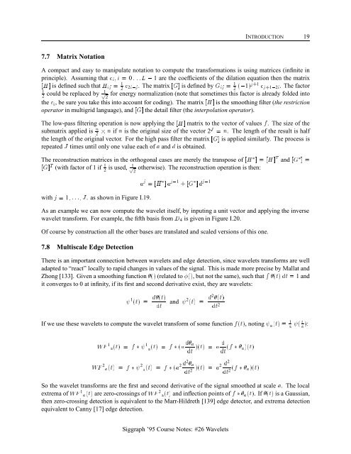
7.7 Matrix Notation
INTRODUCTION 19
A compact and easy to manipulate notation to compute the transformations is using matrices (infinite in
principle). Assuming that ci;i = 0 :::L, 1 are the coefficients of the dilation equation then the matrix
[H] is defined such that Hij = 1
2 c2i,j. The matrix [G] is defined by Gij = 1
2 (,1)j+1 cj+1,2i. The factor
1
1
2 could be replaced by p for energy normalization (note that sometimes this factor is already folded into
2
the ci, be sure you take this into account for coding). The matrix [H] is the smoothing filter (the restriction
operator in multigrid language), and [G] the detail filter (the interpolation operator).
The low-pass filtering operation is now applying the [H] matrix to the vector of values f. The size of the
submatrix applied is n
2 n if n is the original size of the vector 2J = n. The length of the result is half
the length of the original vector. For the high pass filter the matrix [G] is applied similarly. The process is
repeated J times until only one value each of a and d is obtained.
The reconstruction matrices in the orthogonal cases are merely the transpose of [H ]=[H] T and [G ]=
1 is used, p otherwise). The reconstruction operation is then:
2
[G] T (with factor of 1 if 1
2
with j = 1;:::;J. as shown in Figure I.19.
a j =[H ] a j,1 +[G ] d j,1
As an example we can now compute the wavelet itself, by inputing a unit vector and applying the inverse
wavelet transform. For example, the fifth basis from D4 is given in Figure I.20.
Of course by construction all the other bases are translated and scaled versions of this one.
7.8 Multiscale Edge Detection
There is an important connection between wavelets and edge detection, since wavelets transforms are well
adapted to “react” locally to rapid changes in values of the signal. This is made more precise by Mallat and
Zhong [133]. Given a smoothing function () (related to (), but not the same), such that R (t) dt = 1and
it converges to 0 at infinity, if its first and second derivative exist, they are wavelets:
1 (t) =
d (t)
dt
and 2 (t) = d2 (t)
dt 2
If we use these wavelets to compute the wavelet transform of some function f (t), noting a(t) = 1
a
WF 1 a(t) = f 1 a (t) =f (ad a d
)(t) =a
dt dt (f a)(t)
WF 2 a(t) = f 2 a (t) = f (a2 d2 a
d2
)(t) =a2
dt2 dt2 (f a)(t)
So the wavelet transforms are the first and second derivative of the signal smoothed at scale a. The local
extrema of WF 1 a(t) are zero-crossings of WF 2 a(t) and inflection points of f a(t). If (t) is a Gaussian,
then zero-crossing detection is equivalent to the Marr-Hildreth [139] edge detector, and extrema detection
equivalent to Canny [17] edge detection.
Siggraph ’95 Course Notes: #26 Wavelets
( t
a ):