Attitude Determination from GNSS Using Adaptive Kalman Filtering

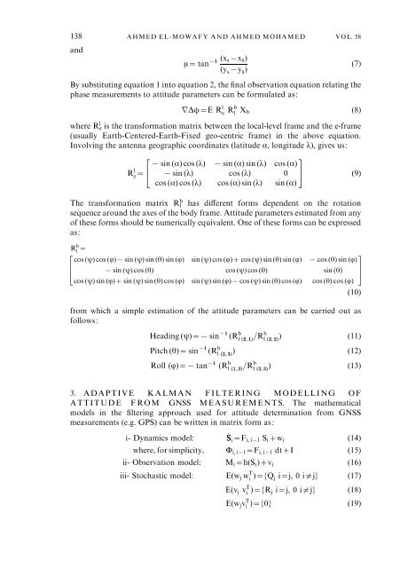
138 AHMED EL-MOWAFY AND AHMED MOHAMED VOL. 58andm= tan (x sxx x1 1 )(y s xy 1 )(7)By substituting equation 1 into equation 2, the final observation equation relating thephase measurements to attitude parameters can be formulated as:rDw=E R l e Rb l X b (8)where R e l is the transformation matrix between the local-level frame and the e-frame(usually Earth-Centered-Earth-Fixed geo-centric frame) in the above equation.Involving the antenna geographic coordinates (latitude a, longitude l), gives us:23x sin (a) cos (l) x sin (a) sin (l) cos (a)R l e = 4 x sin (l) cos (l) 0 5 (9)cos (a) cos (l) cos(a) sin (l) sin (a)The transformation matrix R bl has different forms dependent on the rotationsequence around the axes of the body frame. Attitude parameters estimated from anyof these forms should be numerically equivalent. One of these forms can be expressedas:R b l2=3cos (y) cos (Q)x sin (y) sin (h) sin (Q) sin (y) cos (Q)+ cos (y) sin (h) sin (Q) x cos (h) sin (Q)674 x sin (y)cos(h) cos (y) cos (h) sin (h) 5cos (y) sin (Q)+ sin (y) sin (h) cos (Q) sin (y) sin (Q)x cos (y) sin (h) cos (Q) cos (h) cos (Q)from which a simple estimation of the attitude parameters can be carried out asfollows:(10)Heading (y)=x sin x1 (R b l(2, 1) =Rb l(2, 2) ) (11)Pitch (h)= sin x1 (R b l(2, 3) ) (12)Roll (Q)=x tan x1 (R b l(1, 3) =Rb l(3, 3) ) (13)3. ADAPTIVE KALMAN FILTERING MODELLING OFATTITUDE F ROM GNSS MEASUREMENTS. The mathematicalmodels in the filtering approach used for attitude determination from GNSSmeasurements (e.g. GPS) can be written in matrix form as:i- Dynamics model: Si _ =F i, ixl S i +w i (14)where, for simplicity, W i, ixl =F i, ixl dt+I (15)ii- Observation model: M i =h(S i )+v i (16)iii- Stochastic model: E(w j w T i )={Q j i=j, 0 ilj} (17)E(v j v T i )={R j i=j, 0 ilj} (18)E(w j v T i )={0} (19)