Attitude Determination from GNSS Using Adaptive Kalman Filtering

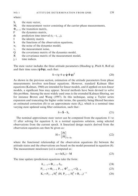
NO. 1 ATTITUDE DETERMINATION FROM GNSS 139where:S i the state vector,M i the measurement vector consisting of the carrier-phase measurements,W i,ix1 the transition matrix,F the dynamics matrix,dt prediction time interval (t i xt ix1 ),I the identity matrixh the functions of the observation equations,w i the noise of the dynamics model,v i the measurement noise,Q the covariance matrix of the dynamics model,R the covariance matrix of the measurement model,j, i time indices.The state vector includes the three attitude parameters (Heading y, Pitch h, Roll Q)and their time rates ( _y _ h _Q), such that:S=(y hQ _y _ h _Q) T (20)As shown in the previous section, estimation of the attitude parameters from phasemeasurements involves non-linear equations. However, standard Kalman filterequations (Kalman, 1960) are intended for linear models, and if applied on non-linearmodels, a significant bias may appear. Several methods have been devised to solvethis problem. Among the most widely used ones is the extended Kalman filtering, seefor instance Brown and Wang (1997). In this technique, using a Taylor seriesexpansion and truncating the higher order terms, the quantity being filtered becomesan estimated correction (d) to an approximate state (S o ), which is a nominal timevarying state updated using filter estimation, such that:d=^SxS o (21)The nominal approximate state vector can be computed from the equations 11 to13 after solving for equation 8, in a normal equations solution, using selectedobservations from the current epoch. A linearized design matrix derived from theobservation equation can then be given as:H= @h (22)@SS=Sowhere the functional relationship of the observation equations (h) between theattitude states and the observations are based on the model presented in equation (8).The measurement misclosure (v) is computed as:v=h(S o )xM (23)The time update (prediction) equations take the form:d i, ix1 =W i, ix1 d i;1 (24)P i, ix1 =W i, ix1 P ix1 W T i, +Q ix1 ix1 (25)K i =P i, ix1 H T i (H i P i, ix1 H T i +R ix1) x1 (26)