Compressive behavior and NDT correlations for chestnut wood ...

More documents

Recommendations

Info

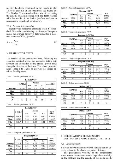
egister the depth penetrated by the needle in planTR or in plan RT of the specimens, see Figure 5b.The Pilodyn 6J was used with the aim of correlatingthe density of each specimen with the depth reachedwith the needle of the device (surface hardness orresistance to superficial penetration).2.3.4 Density determinationDensity was measured according to NP-616 standard.Given the conditioning conditions of the specimens,the average density is determined for a moisturecontent of 12%, given by:m12%r12%= (3)V12%3 DESTRUCTIVE TESTSThe results of the destructive tests, following thegrouping detailed above, are presented taking intoaccount the orientation of the annual growth ringsalong the direction of the force. The tables presentednext (Table 1 to Table 8), provide the values obtainedfor all groups.Table 1. Radial specimens: NCW.Radial (NCW)PoissonE (MPa)νLR νTR νLTσ0,2% (kPa)Average 800,6 0,04 0,32 0,13 7806,9Max. 985,6 0,06 0,39 0,18 10896,8Min. 621,0 0,03 0,21 0,10 5344,8No. 19CV 13 18 12 16 19Table 2. Radial specimens: OCW.E (MPa)Radial (OCW)PoissonνLR νTR νLTσ0,2%(kPa)Average 846,3 0,05 0,32 0,16 8011,6Max. 1058,9 0,08 0,45 0,20 12045,5Min. 562,7 0,04 0,23 0,11 5365,0No. 12CV 17 22 21 15 26Table 3. Diagonal specimens: NCW.Diagonal (NCW)PoissonE (MPa)νLR νTR νLTσ0,2%(kPa)Average 551,5 0,04 0,26 0,16 6233,0Max. 673,1 0,05 0,32 0,19 7400,0Min. 453,8 0,02 0,13 0,12 5224,4No. 20CV 10 22 16 13 10Table 4. Diagonal specimens: OCW.Diagonal (OCW)PoissonE (MPa)νLR νTR νLTσ0,2%(kPa)Average 620,8 0,04 0,26 0,16 6623,1Max. 929,2 0,06 0,32 0,23 9124,8Min. 421,6 0,02 0,21 0,11 4376,3No. 26CV 21 21 12 19 21Table 5. Tangential specimens: NCW.Tangential (NCW)PoissonE (MPa)νLR νTR νLTσ0,2%(kPa)Average 527,6 0,05 0,28 0,18 6667,4Max. 660,2 0,07 0,39 0,23 8792,5Min. 331,0 0,04 0,23 0,16 5170,9No. 18CV 15 17 13 12 14Table 6. Tangential specimens: OCW.Tangential (OCW)PoissonE (MPa)νLR νTR νLTσ0,2%(kPa)Average 572,4 0,06 0,32 0,18 7484,2Max. 687,6 0,08 0,38 0,23 9199,2Min. 467,6 0,05 0,29 0,14 6310,0No. 12CV 12 13 8 13 10Table 7. Diffuse specimens: NCW.Diffuse (NCW)PoissonE (MPa)νLR νTR νLTσ0,2%(kPa)Average 592,7 0,06 0,36 0,17 6523,3Max. 751,8 0,08 0,44 0,22 9307,2Min. 516,0 0,03 0,30 0,07 4684,8No. 22CV 12 19 9 18 16Table 8. Diffuse specimens: OCW.Diffuse (OCW)PoissonE (MPa)νLR νTR νLTσ0,2%(kPa)Average 618,3 0,06 0,35 0,18 6559,6Max. 705,9 0,08 0,43 0,24 7968,0Min. 479,2 0,04 0,29 0,10 4730,4No. 29CV 8 18 9 16 144 CORRELATIONS BETWEEN NON-DESTRUCTIVE AND DESTRUCTIVE TESTS4.1 Ultrasonic testsIt is well known that stress waves velocity can be directlyrelated to the elastic properties of timber.The propagation velocity of the longitudinalstress waves in an elastic media depends essentiallyon the stiffness and the density of the media itself.
On the other hand, it is normally possible to measurethe propagation time of a set of elastic waves in theaxial direction of the wooden elements or in the perpendiculardirections to this (it is stressed again thatthe propagation time is an average time obtainedfrom the measurement of the faster elastic waves).For prismatic, homogeneous and isotropic elementsand for those with section width smaller thanthe stress wavelength, the relation:2Edinv r= ´ (4)holds, where E dinrepresents the dynamic modulusof elasticity (N/mm²); v is the propagation velocityof the longitudinal stress waves (m/s) and r is thedensity of the specimens (kg/m³).For practical purposes, the relation between thedynamic modulus of elasticity and the static valueEmed , staticis particularly relevant ( Edin ³ Emed). Generally(Wood Handbook, 1974), a linear relation isadequate:E = a´ E - b(5)meddinTable 9 to Table 11 provides the values measuredfor all specimens. The obtained values with the ultrasoundtest emphasize the good relation betweenthe dynamic and static moduli of elasticity.Table 9. Dynamic modulus of elasticity (Direct Method, perpendicularto the grain).Dynamic modulus of elasticity (MPa)Direct Method, perpendicular to the grainTangential Diagonal Diffuse RadialNew Old New Old New Old New OldAverage1456 1662 2256 2109 1664 1867 2997 3083No. 19 12 11 16 10 13 18 13CV 16 9 19 18 13 25 19 14Table 10. Dynamic modulus of elasticity (Indirect Method).Dynamic modulus of elasticity (MPa)Indirect MethodTangential Diagonal Diffuse RadialNew Old New Old New Old New OldAverage 12932 12008 12189 13237 13306 12391 13084 12897No. 19 12 11 16 10 13 19 12CV 16 26 14 21 12 16 16 22Table 11. Dynamic modulus of elasticity (Direct Method, parallelto the grain).Dynamic modulus of elasticity (MPa)Direct Method, parallel to the grainTangential Diagonal Diffuse RadialNew Old New Old New Old New OldAverage14445 14540 13368 15091 16057 14601 14445 14525No. 19 12 11 16 10 13 18 13CV 19 22 15 13 13 21 19 22Figure 6 illustrates different correlations obtainedbetween the dynamic modulus of elasticity, takinginto account the orientation of the annual growthrings along the direction of the force, consideringthe Direct Method, perpendicular to the grain, forthe NCW group.Emed (MPa)120010008006004002000Tangentialy = 0,2719x + 166,86R 2 = 0.86Diffusey = 0,2302x + 188,14R 2 = 0.86Diagonaly = 0,3188x - 15,816R 2 = 0.74Radialy = 0,1828x + 293,19R 2 = 0.86500 1500 2500 3500Edin (MPa)TangentialDiagonalDiffuseRadialFigure 6. Relation between Edin and Emed, for the group NCW,using the Direct Method, perpendicular to the grain.4.2 Resistograph testsFigure 7 and Figure 8 show the correlations betweenthe resistographic measure and the density of eachspecimen for the NCW group and for the OCWgroup respectively.Resistographic measure (cm)550450350250150y = 1,0982x - 371,8R 2 = 0.51NCW50500 550 600 650 700Density (kg/m³)Figure 7. Relation between the resistographic measure anddensity (NCW).Resistographic measure (cm)500400300200y = -0,8436x + 779,79R 2 = 0.50OCW100500 550 600 650 700Density (kg/m³)Figure 8. Relation between the resistographic measure anddensity (OCW).
Page 1 and 2: Compressive behavior and NDT correl
Page 3: c,90 (MPa)fc,9050%(a)(b)Arctg Ec,90

Compressive behavior and NDT correlations for chestnut wood ...

Create successful ePaper yourself

Delete template?

Save as template?