Fermat's Little Theorem and a Freshman's Dream

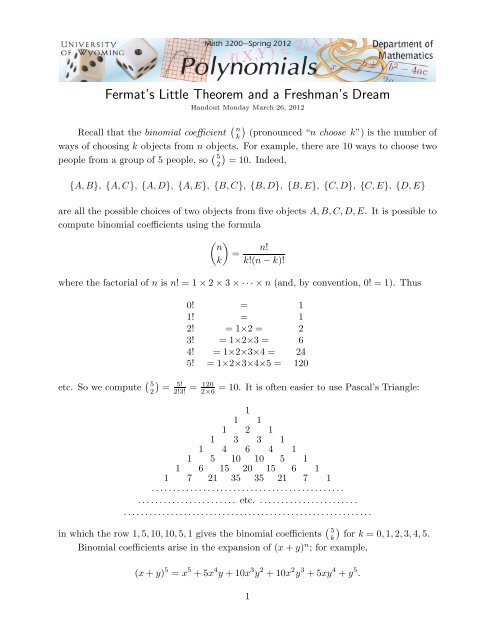
More generally,Theorem 1 (Binomial Theorem). For all n ≥ 0,(x + y) n =n∑k=0( nk)x k y n−k( ) n= x n + nx n−1 y + n(n−1)2x n−2 y 2 + · · · + x k y n−k + · · · + nxy n−1 + y n .kThis theorem may be regarded as expressing a polynomial identity in Z[x,y], where x andy are two indeterminates. Or, we can substitute in numbers for x and y to obtain anotherway of writing (a + b) n for any a,b.An inexperienced or careless person might think that (x+y) n = x n +y n . Amazingly,there are times when this kind of ‘Freshman’s Dream’ actually works! For example, wehave(x + y) 5 = x 5 + y 5 in F 5 [x,y]because the other terms reduce to 0 modulo 5. More generally:Theorem 2 (A Freshman’s Dream). For any prime p, we have the polynomialidentity (x+y) p = x p +y p in F p [x,y]. In particular, for all a,b ∈ Z we have (a+b) p ≡a p + b p mod p.The proof amounts to the fact that the binomial coefficient ( )pk =p!k!(p−k)!is divisible byp for all k ∈ {1,2,... ,p−1} (there is a p in the numerator, and no p in the denominator)whereas ( p0)=( pp)= 1.As a consequence, we exhibit a nonzero polynomial over F p having every element ofF p as a root:Theorem 3. Let p be prime, and consider the polynomial x p − x ∈ F p [x]. Thenevery element a ∈ F p is a root of x p − x. In particular,x p − x = ∏a∈F p(x − a) = x ( x − 1 )( x − 2 ) · · · (x− (p − 1) ) .2

Proof. We must show that a p = a for every a ∈ F p . Clearly 0 p = 0 and 1 p = 1. Next,using our Freshman’s Dream, we observe that2 p = (1 + 1) p = 1 p + 1 p = 1 + 1 = 2;3 p = (2 + 1) p = 2 p + 1 p = 2 + 1 = 3;4 p = (3 + 1) p = 3 p + 1 p = 3 + 1 = 4;etc. Continuing in this way, we get a p = a for all a ∈ F p , i.e. a p − a = 0. Since we have pdistinct roots for x p − x in F p , we have p distinct linear factors andx p − x = x ( x − 1 )( x − 2 ) · · ·(x− (p − 1) ) q(x)for some polynomial q(x) ∈ F p [x]. But the left hand side is monic of degree p, so we musthave q(x) = 1 and the last conclusion follows.Students who have studied proofs by induction will recognize the latter argumentas essentially a proof by induction. Very soon, we will formally introduce mathematicalinduction and point to this as an example.Polynomials vs. Polynomial FunctionsLet’s fix p = 5 for a while. Recall that two different polynomials can give rise to thesame function from F 5 to F 5 ; for example the polynomialsP(x) = x 7 +x 6 +4x 5 +2x 4 +x 3 +3x 2 +x+3 and Q(x) = 2x 6 +2x 5 +2x 4 +2x 3 +2x 2 +3x+3.A table of values for P(x) and Q(x), as functions F 5 → F 5 , is found (most easily usingMaple as demonstrated below):a P(a) Q(a)0 3 31 1 12 2 23 0 04 2 2It should not come as a surprise to find different polynomials representing the samefunction. After all, there are only finitely many different functions f : F 5 → F 5 (5 choicesfor f(0), 5 choices for f(1), ... , and 5 choices for f(4), making 5 × 5 × 5 × 5 × 5 = 3125functions altogether). If different polynomials always represented different functions, thenthere would be at most 3125 different polynomials; whereas in fact, there are infinitelymany different polynomials.3

However, the number of polynomials a 0 + a 1 x + a 2 x 2 + a 3 x 3 + a 4 x 4 of degree lessthan 5 is also 5 5 = 3125. Coincidence? (Not!) Every function F 5 → F 5 is representedby a unique polynomial of degree less than 5, via interpolation. So the interpolation map(giving a polynomial of degree less than 5 for each function F 5 → F 5 ) is in fact bijective,i.e. a one-to-one correspondence.Returning to our polynomials P(x),Q(x) ∈ F 5 [x] above, we divide by x 5 − x andobtain quotient and remainder as follows:P(x) = (x 2 + x + 4)(x 5 − x) + (2x 4 + 2x 3 + 4x 2 + 3)Q(x) = (2x + 2)(x 5 − x) + (2x 4 + 2x 3 + 4x 2 + 3)All of this is most easily checked using Maple:Different quotient, but the same remainder—again, not a coincidence:Theorem 4. Let p be prime, and let P 1 (x),P 2 (x) ∈ F p [x]. Then P 1 (x) and P 2 (x)represent the same function F p → F p , iff they have the same remainder when dividedby x p − x.4

Proof. By the Division Algorithm, we haveP 1 (x) = q 1 (x)(x p − x) + r 1 (x);P 2 (x) = q 2 (x)(x p − x) + r 2 (x)where q i (x),r i (x) ∈ F p [x] and the remainders r 1 (x),r 2 (x) have degree < p. Since x p − xvanishes at every element of F p , the polynomial P 1 (x) has the same values as its remainderr 1 (x); similarly, the polynomial P 2 (x) has the same values as its remainder r 2 (x). So P 1 (x)and P 2 (x) have the same values, iff r 1 (x) and r 2 (x) have the same values, iff r 1 (x) = r 2 (x)(i.e. all coefficients on both sides agree). (Recall that the representation of any functionF p → F p by a polynomial of degree less than p is unique.)If all we ever cared about was infinite fields like Q, R and C, then this matter ofdifferent polynomials representing the same function never arises:Theorem 5. Suppose F is an infinite field. Then two polynomials in F[x] representthe same function, iff they are the same polynomial (i.e. all their coefficients agree).Proof. Suppose two polynomials P 1 (x),P 2 (x) ∈ F[x] represent the same function. Considerthe polynomial h(x) = P 1 (x)−P 2 (x) ∈ F[x]. Then h(a) = P 1 (a)−P 2 (a) = 0 for all a ∈ F,so h(x) has infinitely many roots. If h(x) ≠ 0 then h(x) has at most n roots wheren = degh(x). So we must have h(x) = 0, i.e. P 1 (x) = P 2 (x).Note that a polynomial is zero iff all its coefficients are zero; two polynomials are the sameiff all corresponding coefficients are the same.As promised, this clarifies why different polynomials over R[x] necessarily give differentfunctions; however, this fact is so often taken for granted that even if you only cared aboutthe field of real numbers, the situation for finite fields is a useful reminder that we cannottake Theorem 5 for granted—a proof is required.Finally, just a reminder of another big difference between finite and infinite fields: Overa finite field F, every function F → F is represented by a polynomial (simply interpolate!).Over the real numbers, however, there are lots of functions that are not represented bypolynomials—e.g. sinx and e x are not polynomial functions of x (why?). More generally,if F is any infinite field, then there exist functions F → F that are not represented bypolynomials (why?).In general, therefore, we have three distinct notions:• polynomials;• polynomial functions (i.e. functions represented by polynomials); and• arbitrary functions.5

At certain times in our course, our concern has been with polynomial functions (i.e. functionsrepresented by polynomials); and at other times, we have used polynomials simplyas objects in their own right (remember the decorative spoons!).Application to Primality TestingAn important application of Theorem 3 (usually called Fermat’s Little Theorem)is to primality testing. Let us demonstrate by showing that 51 is not prime (somethingwhat you could check easily enough by directly factoring). If 51 were prime, then byTheorem 3, we would have 6 50 ≡ 1 mod 51. (I chose 6 ∈ {1,2,3,...,50} arbitrarily.)However,6 50 = 808281277464764060643139600456536293376 ≡ 36 mod 51.Since 6 50 ≢ 1 mod 51, we conclude that 51 cannot be prime (although this does not tellus anything about its prime factors). Try this with an actual prime like 53, and we get6 52 = 290981259887315061831530256164353025616435306561536 ≡ 1 mod 53.This is to be expected since 53 is prime.As a second example, we check that the number N = 10 100 + 1 (the number after agoogol) is composite. We cannot ask the computer for a N −1 since this is too big for thecomputer to handle; but we can ask for the answer modulo N since that has at most 100digits. Maple has a syntax for solving this problem, as we now demonstrate:6

For our next example, we consider the number p = 561. We find that a p−1 ≡ 1mod p for many values of a ∈ {1,2,... ,p−1}. However, this does not prove that p isprime. (Fermat’s Little Theorem can yield the conclusion that a number is composite; butit cannot be used to prove that a number is prime.)In this case the number 561 is small enough to be handled by Maple’s integer factorizationcommand ifactor().7

How large a number can Maple factor? If you give it a couple of minutes (dependingon the speed of your computer), you should succeed in factoring the number N = 10 100 +1used above. This is about the limit of Maple’s capability. Most numbers having severalhundred digits are beyond the reach of any computational resources for integer factorizationcurrently available. Testing for primality is much easier, however; computers have notrouble checking whether a given integer (even one having many hundreds of digits) isprime.Prime numbers having several hundreds of digits have important applications in moderncryptography for personal and commercial use. These applications are usually taughtin courses on applied algebra or computational number theory.8