course notes - Self Shadow

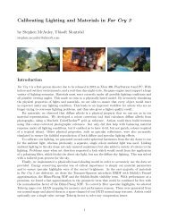
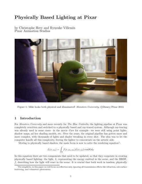
Physically Based Lighting at Pixarby Christophe Hery and Ryusuke VilleminPixar Animation StudiosFigure 1: Mike looks both physical and illuminated! Monsters University, c○Disney/Pixar 2013.1 IntroductionFor Monsters University and more recently for The Blue Umbrella, the lighting pipeline at Pixar wascompletely rewritten and switched to a physically based and ray-traced system. Although ray-tracingwas already used in some cases—in the movie Cars for example—we were still using point lights,shadow maps, ad hoc shading models, etc. Over the years, the original pipeline has gotten more andmore complex, with thousands of lights and shader tweaking in every shot. The idea was to let thecomputer handle all this complexity, freeing the lighter to concentrate on the artistic side.Moving to physically based shaders, the main focus is now to solve the rendering equation 1 :∫L(x, ω o ) = f(x, ω i , ω o )L(x, ω i ) cos(θ)dωΩIn this equation there are two components that need to be updated, so that they cooperate in creatingphysically based lighting: the light, L, representing the energy emitted in the scene, and the BRDF,f, describing how the light will react in the scene. It is crucial that both work in tandem; physically1 For simplicity, in this paper we will focus on reflection only, ignoring all transmission effects like refraction, sub-surfacescattering, and volumetric phenomena.1

correct lights interacting with non-normalized BRDFs, or correct BRDFs interacting with incorrectlights, won’t make much sense. In fact you will probably end up with more disadvantages, withoutseeing the full potential benefits.We typically use Monte Carlo ray-tracing to solve this equation in the general case, but a naiveimplementation would lead to unbearable render times. To avoid this, different strategies are used—depending on what light path we consider—in order to optimize the convergence time. The equationis divided into sub-components, each of which will be resolved by a specific coshader 2 we call anintegrator.∫L(x, ω o ) = f(x, ω i , ω o ) (L direct (x, ω i ) + L indirect (x, ω i )) cos(θ)dω∫ΩL(x, ω o ) = f(x, ω i , ω o )L direct (x, ω i ) cos(θ)dω∫Ω+ (f diffuse (x, ω i , ω o ) + f specular (x, ω i , ω o )) L indirect (x, ω i ) cos(θ)dω∫ΩL(x, ω o ) = f(x, ω i , ω o )L direct (x, ω i ) cos(θ)dω∫Ω+ f diffuse (x, ω i , ω o )L indirect (x, ω i ) cos(θ)dω∫Ω+ f specular (x, ω i , ω o )L indirect (x, ω i ) cos(θ)dωΩThat is:L(x, ω o ) = L direct + L indirectDiffuse + L indirectSpecularL(x, ω o ) radiance from x in the ω o direction [W m −2 sr −1 ]L(x, ω i ) radiance to x in the ω i direction [W m −2 sr −1 ]f s (x, ω i , ω o ) surface BRDF at x from direction ω i to direction ω o [sr −1 ]θangle between the surface normal N and ω i [r]Table 1: NotationsL direct is resolved by the directLighting integrator (light path = E{D,S}L, using [Heckbert 1990]path notation 3 ). L indirectDiffuse is resolved by the indirectDiffuse integrator (light path = ED{D,S}*L),L indirectSpecular by the reflection integrator (light path = ES{D,S}*L). To take advantage of Render-Man’s capabilities, the indirectDiffuse integrator is then divided into sub parts. The caustic integratoris going to solve specular paths ending with a diffuse bounce (EDS*L). For multiple diffuse bounces,we can either use the photon integrator or recursively use the indirect integrator (EDD*L). The photonand caustic integrators make use of photon mapping capability [The RenderMan Team 2013b];the indirectDiffuse integrator uses the radiosity cache (described in [Christensen et al. 2012]) andsome irradiance caching technology.2 A coshader is a specialized object construct in Pixar’s RenderMan: for more information, referto [The RenderMan Team 2009].3 Eye(E), specular(S), diffuse(D), light(L).2

L indirectDiffuse (x, ω o ) ==∫f diffuse (x, ω i , ω o )L indirect (x, ω i ) cos(θ)dω∫Ωf diffuse (x, ω i , ω o )Ω( ∫f specular (x, ω i , ω o )L specular (x, ω i ) cos(θ)dωΩ∫)+ f diffuse (x, ω i , ω o )L diffuse (x, ω i ) cos(θ)dω cos(θ)dωΩThe same recursive algorithm applies for the reflection integrator.Breaking down the equation into parts that are solved by coshader integrators lets us create avery versatile and expandable system, in which we can change parts without rebuilding anything. Forexample, we recently added volumetric integrators; when plugged into our system, everything workedwith minimal changes, since they solve non-overlapping parts of the same problem. You’ll notice thatthere are difficult light paths that we choose to ignore for now; in the future we plan to solve those usingbidirectional path-tracing and vertex merging techniques. We end up with four main integrators 4 :• directLighting integrator• indirectDiffuse integrator• reflection integrator• photonCaustic integratorIn these course notes, we are going to focus on the implementation of the directLighting integrator,which—even in the case of global illumination—represents the major part of the lighting. It is alsothe part we can optimize the most; contrary to indirect integrators that usually don’t 5 have a-prioriknowledge of the scene (before shooting rays into it), the direct lighting integrator knows about thelight sources.The direct lighting computation can be decomposed into three main parts:• Light coshader• BRDF coshader• Integrator coshaderThe integrator coshader is the main shader that will compute the final lighting result using MultipleImportance Sampling (see [Veach and Guibas 1995]). The light and the BRDF shaders are responsiblefor providing all the samples and weights with respect to their sampling strategies. There is a nicesymmetry between the two: they both have a sample function for generating samples using their ownstrategy, and respective emissionAndPDF and valueAndPDF functions to generate values correspondingto the other strategy.We provide many light and BRDF shaders in our library. To name a few, we have: lambertianDiffuse,orenNayarDiffuse, kajiyaHairDiffuse, beckmannIsotropicSpecular, beckmannAnisotropicSpecular,gtrIsotropicSpecular 6 , ggxAnisotropicSpecular and marschnerHairSpecular. For lights, wehave dome 7 , portal, rect, disk, sphere and distant types. As coshaders, they are all abstracted inour system and interchangeable in the scene descriptions.4 Alongside the specialized volumes, transmission and sub-surface scattering integrators.5 See [The RenderMan Team 2013b] for exceptions.6 This is the generalized Trowbridge-Reitz model introduced by [Burley 2012].7 Similar to [Pharr and Humphreys 2004].3

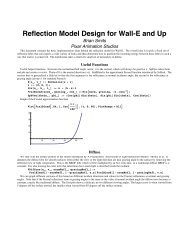
Figure 2: Note the various luminaires in this shot (neon signs, car headlights and various street lights).The Blue Umbrella, c○Disney/Pixar 2013.Figure 3: Different area light types.4

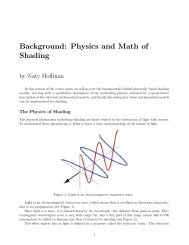
The pieces of data (samples) are passed between these coshaders using structs of arrays:• LightSampleStruct contains the results of the light sampling:sample position P on the lightnormalized vector Ln from the shading point to Psample color Clsample pdf pdf• BSDFSampleStruct contains the results of the BRDF sampling:weighted sample value (value/pdf) weightsample pdf pdfsample direction dir• LightEmissionStruct contains the light-side values of the BRDF sampling:sample position P on the lightsample color Clsample pdf pdf• BSDFValueStruct contains the BRDF-side values of the light sampling:sample value valuesample pdf pdfDirect IntegratorLightSampleStructLightEmissionStructBRDFValueStructBRDFSampleStructsample()sample()LightemissionAndPDF()valueAndPDF()BRDFFigure 4: How the various structures communicate data between the three main coshaders.5

This document will first detail two examples and their implementations: the sphere area lightin section 2 and the beckmannIsotropicSpecular BRDF in section 3. For anyone interested in ourmarschnerHairSpecular approach, we invite you to check [Hery and Ramamoorthi 2012]. Later, insection 4, we will show exactly how the sampling data is pulled together inside our direct integrator.2 Sphere Area LightFigure 5: A nice (sphere) moon scene. Monsters University, c○Disney/Pixar 2013.The sphere area light is our simplest illumination object, and we provide algorithms below for samplingand evaluating this particular luminaire. Originally these functions were written in RenderMan’sShading Language ([The RenderMan Team 1987-2013]); for ultimate performance, we later portedsome of them to C++ (see [Villemin and Hery 2012]) and leveraged Intel’s new ispc compiler—freelyavailable here [Pharr and Mark 2012].6

2.1 Sphere Area Light SamplingFirst (lines 7 to 9), we compute the ideal number of samples, with a heuristic based on the solid angleobserved from the shading point P. Also, from the importance of the ray (rayWeight in the code), wereduce this number of samples in recursion. Then for sampling, we roughly follow [Shirley et al. 1996]—a straightforward approach, where we distribute samples within the solid angle. At lines 14 and 16 ofthe algorithm, we rely on two random numbers 8 : ξ 1 and ξ 2 . If P is inside the light (see lines 3 and 26),no samples are valid.Algorithm 1. (Generating samples from a sphere area light)1void sample (out LightSamplingStruct ls)// Check whether we are inside or not2 vector lightCenterDir = lightCenterPos − P;3 float d2 = lightCenterDir · lightCenterDir;4 if (d2 − radius 2 ) ≥ 1e-4 thenfloat d = √ 5d2;// Build an orthonormal basis towards the center of the sphere6 vector ONBU, ONBV, ONBW;7 CreateBasisFromW (lightCenterDir / d, ONBU, ONBV, ONBW);89101112131415161718// Determine desired number of samples, between min and max and handle recursion√d2float solidAngle = 1 −; // Actually, the solid angle is 2π times this quantityradius 2 +d2int numSamples = ceil(rayWeight ∗ solidAngle ∗ (maxSamples − minSamples));ls → numValid = numSamples;√float costhetamax = 1 − radius2d2;float pdf = 1/(2π ∗ (1 − costhetamax));for int i = 0; i < numSamples; i += 1 dofloat costheta = 1 + ξ 1 [i] ∗ (costhetamax − 1);float sin2theta = 1 − costheta 2 ;vector lightDir = SphericalDir( √ sin2theta, costheta, 2π ∗ ξ 2 [i]);lightDir = TransformFromBasis(lightDir, ONBU, ONBV, ONBW);√float ∆ = radius 2 − sin2theta ∗ d2 ;19 ls → P[i] = P + (costheta ∗ d − ∆) ∗ lightDir;20 ls → Ln[i] = lightDir;21 ls → pdf[i] = pdf;22 ls → Cl[i] = lightColor;23 end24 end25 else26 ls → numValid = 0;27 end8 These numbers can, for instance, be generated via [Kensler 2013].7

2.2 Sphere Area Light EvaluationHere is the evaluation method of the light, given an array of BRDF samples as input. We use a simplequadratic formula, lines 15-19, to check on the potential hits to the light. If a given BRDF sampledirection does not see the light (through this intersection routine), we mark the record with a PDFvalue of 0 (line 30).Algorithm 2. (Evaluating BRDF samples on a sphere area light)1void emissionAndPDF (in BSDFSamplingStruct bs; out LightEmissionStruct le)2 if bs → numValid = 0 then3 return;4 end// Check whether we are inside or not5 vector lightCenterDir = P − lightCenterPos;6 float d2 = lightCenterDir · lightCenterDir;7 if (d2 − radius 2 ) ≥ 1e-4√then8 float costhetamax = 1 − radius2d2;9 float pdf = 1/(2π ∗ (1 − costhetamax));// intersect light10 for int i = 0; i < numValid; i += 1 do11 boolean isValid = false;12 vector dir = bs → dir[i]; // direction towards the light13 float b = 2 ∗ dir · lightCenterDir;14 float c = lightCenterDir · lightCenterDir − radius 2 ;15 float ∆ = b 2 − 4 ∗ c;16 if ∆ > 0 thenfloat t = −b−√ ∆172;18if t < 1e-5 thent = −b+√ ∆192;20end21if t ≥ 1e-5 and t ≤ 1e20 then// we have a hit22isValid = true;23le → P[i] = P + t ∗ dir;24le → Cl[i] = lightColor;25le → pdf[i] = pdf;26end27 end28 if isValid = false then29le → Cl[i] = color(0);30le → pdf[i] = 0;31 end32 end33 end8

2.3 Sphere Area Light Diffuse ConvolutionThis function is used in the integrator for the control variates method (refer to 4.5). We follow [Snyder 1996].Note that we check on the surface type to determine whether we can provide a valid convolution or not.Algorithm 3. (Diffuse convolution of a sphere area light)1boolean diffConvolution (out color diffConv)// Check whether we can provide a diffuse convolution to the integrator2 if enableControlVariates = false or isHair = true then3 return false;4 end5diffConv = color(0);6 if lightColor ! = color(0) then// Check whether we are inside or not7 vector lightCenterDir = lightCenterPos − P;8 float d2 = lightCenterDir · lightCenterDir;9 float cosTheta = lightCenterDir·N √d2;1011121314if (d2 − radius 2 ) ≥ 1e-4 thenfloat sinAlpha = radius √d2;float cosAlpha = √ 1 − sinAlpha 2 ;float alpha = asin(sinAlpha);float theta = acos(cosTheta);18// we use the faster cubic formula15 if theta < ( π 2− alpha) then16diffConv = cosTheta ∗ sinAlpha 2 ;17 endelse if theta < π 2 then19float g0 = sinAlpha 3 ; // dfloat g1 = 1 π∗ (alpha − cosAlpha ∗ sinAlpha);21float gp0 = −cosAlpha ∗ sinAlpha 2 ∗ alpha; // c22float gp1 = −sinAlpha 2 ∗ alpha/2;23float a = gp1 + gp0 − 2 ∗ (g1 − g0);24float b = 3 ∗ (g1 − g0) − gp1 − 2 ∗ gp0;float y = (theta − ( π 2 − alpha))/alpha;26diffConv = g0 + y ∗ (gp0 + y ∗ (b + y ∗ a)); // ay 3 + by 2 + cy + d27 end28 else if theta < ( π 2+ alpha) thenfloat g0 = 1 π∗ (alpha − cosAlpha ∗ sinAlpha); // d30float gp0 = −(sinAlpha 2 ∗ alpha)/2; // c31float a = gp0 + 2 ∗ g0;32float b = −3 ∗ g0 − 2 ∗ gp0;float y = (theta − π 2 )/alpha;34diffConv = g0 + y ∗ (gp0 + y ∗ (b + y ∗ a)); // ay 3 + by 2 + cy + d35 end// else leave diffConv at 036 end37 diffConv *= lightColor;38 end39return true;9

3 Beckmann BRDFThis particular specular model was derived with a view towards simplicity and efficiency. It is largelyinspired by [Walter et al. 2007], and also has much in common with the grand-daddy of all models:[Cook and Torrance 1982].We decided to employ the trusted Beckmann distribution, with a roughness term α (between 0 and1). For an arbitrary microfacet normal m, using θ m as the angle between this m direction and themacroscopic surface normal n, the distribution is expressed as:D b (m) = e− tan2 (θ m)/α 2π α 2 cos 4 (θ m ) =e (n·m)2 −1α 2 (n·m) 2π α 2 (n · m) 4As we saw in [Hoffman 2013], microfacet BRDFs always evaluate normal distributions at h, the halfwayvector from the light direction l and the view direction v. [Walter 2005] derives a sampling strategy forthe dominant term in D b , i.e. the exponential. In this scheme, each sample is picked with a probability:pdf = D b(h) (n · h)4 (v · h)Suppose we have our full BRDF model (which has many terms in addition to D b ), and use “value” todenote its evaluation for a given set of l, v and n (and consequently h). By definition of radiance andsampling, we have:value (n · l)color =pdfOne desirable property of a BRDF model in a production environment is that it preserves energy asmuch as possible. A common verification method is the “white furnace” test 9 , which should producea uniformly white result. Mathematically, this translates to:In other words:value (n · l)pdf= 1f µ (l, v) = value = pdfD b (h) (n·h)n · l = 4 (v·h)n · lAccounting for Fresnel, F , this gives us our BRDF:f µ (l, v) = F (l, h) D b(h) (n · h)4 (n · l) (v · h)= D b(h) (n · h)4 (n · l) (v · h)In practice, we pull out the Fresnel term from this definition and incorporate the regular n · l cosineinstead. This cancels out, leaving:f ∗ µ(l, v) = D b(h) (n · h)4 (v · h)= pdfThis has the advantage of being a very simple (and fast) expression and it also guarantees that wepass the furnace test, at least as far as the Beckmann distribution goes. With small roughness values,say α ≤ 0.1, D b (and thus f µ ) will indeed abide by the furnace requirement. For larger values, we stilllose some energy at grazing angles. This is the reason for pulling the Fresnel term out: artists can useit to compensate for the loss. In summary, our BRDF (with built-in cosine) is:f ∗ µ(l, v) =e (n·h)2 −1α 2 (n·h) 24 π α 2 (n · h) 3 (v · h)A perfect Distribution-based BRDF! (See [Ashikhmin and Premoze 2007].)9 A pure white object is uniformly lit without shadows under a pure-white dome.10

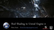
Figure 6: Beckmann specular: increasing roughness values from 0.001 to 1.03.1 Beckmann BRDF samplingNow that we have our target distribution, we show how BRDF samples are generated using that distribution.Note that we do not enforce energy conservation between the various lobes: this is left asan “exercise” for the shading artist, who has to guarantee (or not) that the sum of the K terms is ≤ 1.In the algorithms below, it is assumed that Fresnel is baked externally into specColor and that thefacing-ratio test, V·Ng, has been done prior to the call. Lines 8 and 14 are directly from [Walter 2005].Algorithm 4. (Sampling of a Beckmann specular lobe)1void sample (in vector wi; in int lobeSamples; out BSDFSamplingStruct bs)// Note that we already rejected earlier the cases where V · Ng < 02 if specColor = color(0) or lobeSamples = 0 then3 return; // no need to sample4 end56// Need to rectify the probabilities from the fact that I am sampling all lobes at oncefloat ratio = bs → numSamples/lobeSamples;int numCurrent = bs → numValid; // we will add to the list from there7 for int i = 0; i < lobeSamples; i += 1 do// Sample angle theta8 float tantheta2 = − ln ξ 1 [i] ∗ roughness 2 ;19 float costheta = √ 1+tantheta2;1011121314151617181920// Create a halfvector√vector H = SphericalDir( 1 − costheta 2 , costheta, 2π ∗ ξ 2 [i]);float VdotH = wi · H;// Compute incident direction by reflecting about Hvector wo = −wi + 2 ∗ VdotH ∗ H;if wo · N > 0 then// ξ 1[i] represents the Beckmann exponential termξbs → pdf[numCurrent] =1[i]∗ratio4π∗costheta 3 ∗roughness 2 ∗abs(VdotH) ;// weight = value∗LdotN , which becomes by design:pdfbs → weight[numCurrent] = specColorratio;// Corresponding sampling directionbs → dir[numCurrent] = wo;numCurrent += 1;endendbs → numValid = numCurrent;11

3.2 Beckmann BRDF evaluationOur BRDF must also be able to evaluate the contribution of samples generated from the lightingdistribution. Some light samples may resolve to zero contribution, because they face the wrong way(line 17). Also, remember that our returned value at line 13 is actually the product of the BRDF bythe cosine.Algorithm 5. (Evaluation of a beckmann specular lobe)1boolean valueAndPDF (in vector wi; in vector wos[]; out BSDFValueStruct bv)2 boolean hasValidValues = false;// Note that we already rejected earlier the cases where V · Ng < 03 if specColor = color(0) then4 return hasValidValues; // no valid values5 end6 for int i = 0; i < bv → numSamples; i += 1 do7 vector wo = wos[i];891011if wo · N > 0 thenhasValidValues = true;// Compute the microfacet distribution (Beckmann)vector H = normalize(wo + wi);float costheta = H · N;costheta 2 −112 float pdf = eroughness 2 ∗costheta 2 /(4π ∗ costheta 3 ∗ roughness 2 ∗ (wi · H));13 bv → value[i] = specColor ∗ pdf;14 bv → pdf[i] = pdf;15 end16 else17 bv → value[i] = color(0);18 bv → pdf[i] = 0;19 end20 end21 return hasValidValues;12

4 Direct lighting integratorThe directLighting integrator will gather all the samples from the BRDF coshaders and the lightcoshaders, and will compute the final result. For robustness, we combine these two sampling strategiesusing Multiple Importance Sampling (MIS). As described in the introduction, this integrator focuses ondirect lighting only, so the computation is optimized for this sole task, completely ignoring all indirecteffects. Since the BRDF’s sampling is independent of the lights, it is done once outside of the lightloop. Notice that we return two BSDFSampleStructs here, one for “normal” area lights and one forinfinite lights (see 4.3). Depending on the light type we will use bs or bsbvh. The bsbvh will onlycontain samples that are hitting at least one light. We still need the original sets of samples for infinitelights that are potentially hit by any direction. Then the results for all lights are accumulated intothe final result. One important point here is that although we have area lights, by default they don’thave any geometric representation in the scene and thus are not themselves visible. This is also whywe have a separate acceleration structure for those lights.Algorithm 6. (Direct Lighting Integration)12color integrate ()// Get BSDF samples -- sample according to BRDF strategyIntegrateBrdf(bs, bsbvh, numSpecLobes, numSpecSamples);// Light loop3 for int l = 0; l < lightCount; l += 1 do4 shader li = lights[l];5678910// Get Light samples -- sample according to Light strategyif li → hasInfiniteBounds thenIntegrateLight(li, bs, numSpecLobes, numSpecSamples, finalDiff, finalSpec);endelseIntegrateLight(li, bsbvh, numSpecLobes, numSpecSamples, finalDiff, finalSpec);end11 resultDiff += finalDiff;12 resultSpec += finalSpec;13 result += finalDiff + finalSpec;14 end15 return result;13

4.1 BSDF StructThe BSDFStruct is a structure that contains all of the BRDF lobes for a given material 10 . We combinethem in this struct for code clarity, and also for performance reasons. For diffuse components, inorder to optimize computation, we “flatten” all the lobes into one, by using a merged albedo insteadof multiple different albedos (if the lobes are standard Lambertian diffuse). Even if we have morecomplicated (potentially view-dependent) diffuse, we still have a gain by sampling all the lobes at onceusing a single strategy—uniform or cosine-weighted, for example. For specular lobes, since they eachwill use a different strategy (either because it is a set of distinct BRDF models or if they have differentroughnesses), we need to sample them separately, but we can still store all the samples in one commonstruct. Once we have all the samples and their corresponding values and PDFs, we don’t really need toknow where and how they were computed: the values are enough to perform MIS. valueAndPDF Specis shown here, valueAndPDF Diff is equivalent:Algorithm 7. (BSDFStruct valueAndPDF Spec)1void valueAndPDF Spec (out BSDFValueStruct bv)2 for int i = 0; i < numSpecularBRDFs; i += 1 do3 boolean hasValidValues = specularBRDFs[i] → valueAndPDF(wi, wouts, onebv);4 if hasValidValues = false then5 int numDirections = arraylength(wouts);6 for int k = 0; k < numDirections; k += 1 do7onebv → value[k] = color(0);8onebv → pdf[k] = 0;9 end10 end11 push(bv, onebv);// one struct of arrays per lobe for MIS on specular12 endAlgorithm 8. (BSDFStruct sample)1void sample ()// Sample each specular BRDF2 for int i = 0; i < numSpecularBRDFs; i += 1 do3 int thisNumSamples = specularSamples[i];4 if thisNumSamples > 0 and facingRatio ≥ 0.0 then5 specularBRDFs[i] → sample(wi, thisNumSamples, bs);6 end7 end10 If this was not obvious, let’s state here that our materials can contain arbitrary numbers of lobes, each of arbitrarytypes.14

4.2 Light integratorThis is the integration code for a single light. We assume that the BRDF sampling has already beendone outside and has been passed here as an input parameter. First we compute the samples accordingto the light strategy. This is done using the sample function in the light coshader (as in section 2.1).Then, in order to use MIS, we will compute the corresponding values and PDFs for BRDF sampling.This is done through the emissionAndPDF function, that takes the valueAndPDF function for each ofthe BRDF coshaders. These will give us the first pair of values. Next we compute the correspondinglight values for the BRDF samples that were passed as inputs. Since the BRDF sampling was alreadydone outside, we only need to call the emissionAndPDF on the light coshader side. This, combinedwith the input samples of the BRDF, will give us the second pair of values for MIS.The computeMIS function will then calculate the final values and weights for each of those samples.At this stage we have the results without any visibility taken into account. The final step is to computethe visibility term for all the resulting samples. Shadowing is done at the very end because it is usuallythe most expensive step, and doing it after everything enables to use the final weighting of each sampleto optimize its computation using a cutoff (or Russian Roulette if we want to stay unbiased). This isalso true if we have enabled resampling: the final number of samples will be reduced before doing theshadowing calculation.Algorithm 9. (Light Integration)1 color integrateLight (shader li; out BSDFSamplesStruct bs; out int numSpecLobes; out intnumSpecSamples; out color lightDiff, lightSpec)2// Light samplingli → sample(ls);// Check generated samples3 int numGeneratedLightSamples = ls → numValid;4 int numActiveSpecSamples = bs → numValid;// BRDF evaluation5 if numGeneratedLightSamples > 0 then// No MIS on diffuse: do all diffuses together6 bsdf → valueAndPDF Diff(diffValues);// On the other hand, return an array for the specular lobes7 bsdf → valueAndPDF Spec(specValues);8 end910// Light evaluationli → emissionAndPDF(bs, lightValues);// Importance samplingcomputeMIS(ls, diffValues, specValues, bs, lightValues, Cdiff, Cspec, CspecBRDF);// Light shadows11 if numGeneratedLightSamples > 0 then12 computeLightShadows(Cdiff, Cspec, diffPerLight, diffPerLightNoShad, specPerLight, specPerLightNoShad);13 end// BRDF shadows14 if numActiveSpecSamples > 0 and facingRatio ≥ 0.0 then15 computeBRDFShadows(CspecBRDF, specPerLight, specPerLightNoShad);16 end// Per light integration output17 lightDiff = mix(diffPerLightNoShad, diffPerLight, shadowDensity);18 lightSpec = mix(specPerLightNoShad, specPerLight, shadowDensity);15

4.3 BRDF integratorThe BRDF’s integration is done for all the specular lobes at once. The number of lobes is returnedin numSpecLobes, and the number of samples per lobe is returned in an array numLobeSamples. EachBRDF can have a variable number of samples based on its properties (roughness, etc.). An optimizationis performed at that stage: all the samples are tested against an acceleration structure containing allof the area lights. If a BRDF sample does not hit any light, it is discarded. This optimization is notrequired, but is recommended as the sampling can become very expensive if you have thousands oflights in the scene. We still keep the original set of samples, to use against infinite lights (dome arealight in particular); the direct lighting integrator is responsible for passing the right sample set to thelight depending on its type.Algorithm 10. (BRDF Integration)1 color integrateBrdf (out BSDFSamplesStruct bs; out BSDFSamplesStruct bsbvh; out int numSpecLobes;out int numSpecSamples)234567// Get BSDF samples -- sample according to BRDF strategybsdf → getNumSpecSamples(numLobeSamples, numSpecSamples);numSpecLobes = arraylength(numLobeSamples);if numSpecLobes > 0 thenbs = bsdf → sample();// Early reject BRDF samples (through bvh query) that do not intersect any lightsbsbvh = BVHReduce(P, bs);end(a) Light integration result(b) BRDF integration resultFigure 7: Two sampling strategies16

4.4 MIS integratorOnce we have all the samples from the two strategies—Light and BRDF—we can perform MIS. (Fordiffuse lobes, we usually only use light sampling 11 .) Our integrator also has the possibility to perform aresampling step 12 , or resampled MIS (as in [Talbot et al. 2005]) in the case of MIS. This is sometimesuseful to reduce the number of shadow rays to trace, especially if a lot of samples were necessary tosolve a high frequency pattern in the emission of the light.Algorithm 11. (Compute MIS)1 color computeMIS (LightSampleStruct ls; BSDFValueStruct diffValues; BSDFValueStruct specValues;BRDFStruct bs; LightEmissionStruct lightValues; out color Cdiff, Cspec, CspecBRDF)2 if diffResampPercentage ≥ 1.0 then3 integrateIS(diffValues, ls, Cdiff);4 end5 else6 integrateRIS(diffResampPercentage, diffValues, ls, Cdiff);7 end8 if facingRatio ≥ 0.0 then9 if specResampPercentage ≥ 1.0 then10 integrateMIS(ls, specValues, numLobeSamples, Cspec, bs, lightValues, CspecBRDF);11 end12 else13 integrateRMIS(specResampPercentage, ls, specValues, numLobeSamples, Cspec, bs, lightValues, CspecBRDF);14 end15 end(a) with shadowing(b) without shadowingFigure 8: MIS integration result11 We still might want to perform MIS even on diffuse lobes when a light source is very close to the shading point. Inthat case, the light sampling integral has a peak because of the division by the squared distance. Using BRDF samplingwill get rid of this singularity.12 Because the resampling can be costly, we do this in an optimized DSO, which in RSL is a specialized function directlywritten in C/C++ to expand the language or for performance gains.17

4.5 Shadow integratorLight shadowing is done using ray-tracing of transmission (shadow) rays that are optimized to onlycompute visibility. This is not shown here, but specialized shadowing strategies can be implementedhere. As long as the strategies do not overlap each other (i.e., not creating double shadows), we canhave multiple calls to different shadowers. For example, after shadow tracing against standard objectsin the scene, one can use a specialized Spherical Harmonics visibility scheme for heavy vegetation,and/or ray-march inside shadow maps for large hair objects (see [The RenderMan Team 2011]).An additional step is done using control variates 13 if the light was able to provide an analyticalsolution of its non-shadowed lighting. This usually relies on a contour integral computation or atexture map pre-convolution. Common techniques, albeit somehow approximate, to obtain a diffuseconvolution can make use of a Spherical Harmonics representation ([Ramamoorthi and Hanrahan 2001]and [Mehta et al. 2012]). Refer to 2.3 for an example on our Sphere area light.The idea here is that we want to calculate:∫I = fvwith f being the product of the incoming radiance and the BRDF, and v, the visibility term. Withoutany changes, I can be rewritten as:∫ (∫ ∫ )I = fv + α f − f , ∀αIf we have a way to calculate analytically G = ∫ f, this leads to:∫I =( ∫fv + α G −For instance, we can take α = ¯v, the average visibility. The advantage is that if ¯v is 1 (i.e., v is 1everywhere), then I is exactly G. On the other hand, if ¯v is exactly 0, then I is the original sampling.If ¯v is between 0 and 1, there is still variance reduction, as long as the correlation between f and fvis high enough. Here:• G is our diffuse preconvolved solution, diffConv• ∫ fv is diffPerLight• ∫ f is diffPerLightNoShadWe direct the reader to [Clarberg and Akenine-Möller 2008], which describes a strategy for estimatingan approximate and efficient ¯v term.13 A classic Monte Carlo technique well documented in [Kalos and Whitlock 1986].)f18

(a) Control variates off(b) Control variates onFigure 9: Control variates on diffuse. Observe the reduction of variance in the non-shadowed regions.Algorithm 12. (Compute Light Shadows)1 color computeLightShadows (color Cdiff[], Cspec[]; out color diffPerLight, diffPerLightNoShad,specPerLight, specPerLightNoShad)2 color Lvis[];3 avgVis = AreaShadowRays(ls → P, ls → pdf, Lvis);4 for int i = 0; i < numGeneratedLightSamples; i += 1 do5 diffPerLight += Cdiff[i] ∗ (color(1) − Lvis[i]);6 diffPerLightNoShad += Cdiff[i];7 end8 if facingRatio ≥ 0.0 then9 for int i = 0; i < numGeneratedLightSamples; i += 1 do10 specPerLight += Cspec[i] ∗ (color(1) − Lvis[i]);11 specPerLightNoShad += Cspec[i];12 end13 end// Check diffuse convolution14 if li → diffuseConvolution(diffConv) = true then// Do control variates15 diffConv *= bsdf → albedo();16 diffPerLight += (color(1) − avgVis) ∗ (diffConv − diffPerLightNoShad);17 diffPerLightNoShad = diffConv;18 endBRDF shadowing is straightforward: there is no special trick here, we just trace all the shadowrays and add the results to the specular accumulation. The same method applies here if we want touse multiple shadowing strategies (SH, shadow maps, etc.), i.e. this is the place to run them.19

Algorithm 13. (Compute BRDF Shadows)1 color computeBRDFShadows (color CspecBRDF[]; out color specPerLight, specPerLightNoShad)2 color LvisBRDF[];3 color AreaShadowRays(lightValues → P, bs → pdf, LvisBRDF);4 for int i = 0; i < numActiveSpecSamples; i += 1 do5 specPerLight += CspecBRDF[i] ∗ (color(1) − LvisBRDF[i]);6 specPerLightNoShad += CspecBRDF[i];7 end5 ConclusionRenderMan’s versatility allows the shader writer to create his very own integrators, lights and BRDFs.One can thus develop a full physically based system—such as what we outlined in this document—without touching at the guts of the renderer. However, if you don’t need this level of customization,or simply want the render engine to take care of all the implementation details and performance optimization,you can use the built-in integrators of RenderMan 17.0 [The RenderMan Team 2012], andthe new geometric arealights API in RenderMan 18.0 [The RenderMan Team 2013a].We want to acknowledge here the work of all the shading, lighting and rendering artists on MonstersUniversity and The Blue Umbrella, and in particular want to thank their respective Directors ofPhotography (Jean-Claude Kalache on Monsters University and Brian Boyd for The Blue Umbrella).We also want to express our gratitude to the full RenderMan team and to the group of TDs that werepart of the “GI” project.Quote from Jean-Claude Kalache, the lighting Director of Photography on Monsters University:“Physically based lights simplified our setups dramatically. Our master lighting productivity doubledand our shot lighting efficiency went up by 55%. We used multi-threading for interactive and batchrenders. The overwhelming feedback we got from lighters was that the new lights were easy to useand provided more time for artistic exploration. We also used the physically based lights to createmeaningful pre-vis lighting for the Sets Shading department. Every major set was pre-vised with theselights on average in 1-2 days. We used IBL 14 techniques for the Character department, providing halfa dozen lighting setups. The lighting setups for both departments were normalized, which resulted inmore robust shader behavior under any lighting conditions.”Quote from Chris Bernardi, the set shading lead on Monsters University:“Physical shading required us to unify Specular and Reflection from the shading side: we had to rethinkmany long-held approaches, but the result was a more coherent representation of specular acrossour sets. There were far fewer adjustments that needed to be made in the context of lighting andour materials became far more portable as a result. A secondary result, was that since the lightingrigs became simpler to work with, it was easier for Lighting to deliver customized lighting setups forindividual sets. This gave us the opportunity to fine tune our shaders in the context of some meaningfullighting, which also helped us deliver cleaner shading inventory in return. The combination ofrendering with HDR 15 and the energy conservation of the specular model made it easier to hit a widervariety of materials and most of the tweaking was primarily with the roughness control.”14 Image Based Lighting: this is the illumination mode triggered by our dome area light15 High Dynamic Range texture on the dome light20

Figure 10: Monsters University: daylight scene c○Disney/Pixar 2013Figure 11: The Blue Umbrella: nightime rainy scene c○Disney/Pixar 201321

References[Ashikhmin and Premoze 2007] Ashikhmin, M., and Premoze, S. 2007. Distribution-basedBRDFs. Tech. rep., Program of Computer Graphics, Cornell University.[Burley 2012] Burley, B., 2012. Physically-based shading at Disney. http://selfshadow.com/s2012-shading/.[Christensen et al. 2012]Christensen, P. H., Harker, G., Shade, J., Schubert, B.,and Batali, D., 2012. Multiresolution radiosity caching for efficientpreview and final quality global illumination in movies.http://graphics.pixar.com/library/RadiosityCaching/.[Clarberg and Akenine-Möller 2008] Clarberg, P., and Akenine-Möller, T. 2008. ExploitingVisibility Correlation in Direct Illumination. Computer GraphicsForum (Proceedings of EGSR) 27, 4.[Cook and Torrance 1982]Cook, R. L., and Torrance, K. E. 1982. A reflectance modelfor computer graphics. ACM Trans. Graph. 1, 1 (Jan.), 7–24.[Heckbert 1990] Heckbert, P. S. 1990. Adaptive radiosity textures for bidirectionalray tracing. SIGGRAPH Comput. Graph. 24, 4 (Sept.),145–154.[Hery and Ramamoorthi 2012][Hoffman 2013]Hery, C., and Ramamoorthi, R. 2012. Importance samplingof reflection from hair fibers. Journal of Computer Graphics Techniques(JCGT) 1, 1 (June), 1–17.Hoffman, N., 2013. Background: Physics and math of shading.http://selfshadow.com/s2013-shading/.[Kalos and Whitlock 1986] Kalos, M. H., and Whitlock, P. A. 1986. Monte CarloMethods. John Wiley Sons.[Kensler 2013] Kensler, A. 2013. Correlated multi-jittered sampling. Tech.Rep. TM-13-01, Pixar Animation Studios.[Mehta et al. 2012][Pharr and Humphreys 2004][Pharr and Mark 2012]Mehta, S. U., Ramamoorthi, R., Meyer, M., and Hery,C. 2012. Analytic tangent irradiance environment maps foranisotropic surfaces. Comp. Graph. Forum 31, 4 (June), 1501–1508.Pharr, M., and Humphreys, G., 2004. Infinite area light sourcewith importance sampling. http://www.pbrt.org/plugins/infinitesample.pdf.Pharr, M., and Mark, W. R., 2012. ispc: A SPMD compilerfor high-performance cpu programming. http://llvm.org/pubs/2012-05-13-InPar-ispc.html.[Ramamoorthi and Hanrahan 2001] Ramamoorthi, R., and Hanrahan, P. 2001. An efficientrepresentation for irradiance environment maps. In Proceedings ofthe 28th annual conference on Computer graphics and interactivetechniques, ACM, New York, NY, USA, SIGGRAPH ’01, 497–500.22

[Shirley et al. 1996]Shirley, P., Wang, C., and Zimmerman, K. 1996. Monte carlotechniques for direct lighting calculations. ACM Trans. Graph. 15,1 (Jan.), 1–36.[Snyder 1996] Snyder, J. M. 1996. Area light sources for real-time graphics.Tech. Rep. MSR-TR-96-11, Microsoft Research, AdvancedTechnology Division, Microsoft Corporation, One Microsoft Way,Redmond, WA 98052.[Talbot et al. 2005]Talbot, J. F., Cline, D., and Egbert, P. K. 2005. Importanceresampling for global illumination. In Proc. EGSR.[The RenderMan Team 1987-2013] The RenderMan Team, 1987-2013. Shading language(RSL). http://renderman.pixar.com/resources/current/rps/shadingLanguage.html.[The RenderMan Team 2009] The RenderMan Team, 2009. Shader objects and coshaders.http://renderman.pixar.com/resources/current/rps/shaderObjects.html.[The RenderMan Team 2011] The RenderMan Team, 2011. Area shadowing support.http://renderman.pixar.com/resources/current/rps/areaShadow.html.[The RenderMan Team 2012]The RenderMan Team, 2012. Physically plausible shading inRSL. http://renderman.pixar.com/resources/current/rps/physicallyPlausibleShadingInRSL.html.[The RenderMan Team 2013a] The RenderMan Team, 2013. Geometric area lights.http://renderman.pixar.com/resources/current/rps/geometricAreaLights.html.[The RenderMan Team 2013b] The RenderMan Team, 2013. New photon mapping features.http://renderman.pixar.com/resources/current/rps/newPhotonMapping.html.[Veach and Guibas 1995] Veach, E., and Guibas, L. J. 1995. Optimally combiningsampling techniques for monte carlo rendering. In Proceedings ofthe 22nd annual conference on Computer graphics and interactivetechniques, ACM, New York, NY, USA, SIGGRAPH ’95, 419–428.[Villemin and Hery 2012] Villemin, R., and Hery, C., 2012. Porting RSL toC++. http://renderman.pixar.com/resources/current/rps/portingRSLtoC.html.[Walter et al. 2007][Walter 2005]Walter, B., Marschner, S. R., Li, H., and Torrance,K. E. 2007. Microfacet models for refraction through roughsurfaces. In Proceedings of the 18th Eurographics conference onRendering Techniques, Eurographics Association, Aire-la-Ville,Switzerland, Switzerland, EGSR’07, 195–206.Walter, B. 2005. Notes on the Ward BRDF. Tech. Rep. PCG-05-06, Program of Computer Graphics, Cornell University.23