Diversity of Small Mammals in the Pacific Coastal Desert of Peru ...

More documents

Recommendations

Info

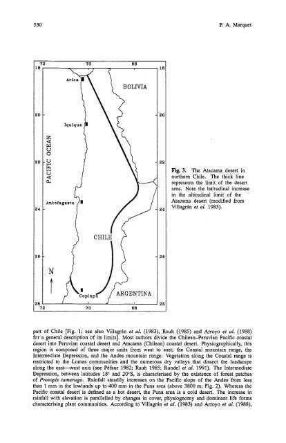
P. A. MarquetIquique3Wv02kv4aFig. 3. The Atacama desert innorthern Chile. The thick linerepresents the limit of the desertarea. Note the latitudinal increasein the altitudinal limit of theAtacama desert (modified fromVillagrfin et al. 1983).part of Chile [Fig. 1; see also Villagrin et al. (1983), Rauh (1985) and Arroyo et al. (1988)for a general description of its limits]. Most authors divide the Chilean-Peruvian Pacific coastaldesert into Peruvian coastal desert and Atacama (Chilean) coastal desert. Physiographically, thisregion is composed of three major units from west to east; the Coastal mountain range, theIntermediate Depression, and the Andes mountain range. Vegetation along the Coastal range isrestricted to the Lomas communities and the numerous dry valleys that dissect the landscapealong the east-west axis (see PCfaur 1982; Rauh 1985; Rundel et al. 1991). The IntermediateDepression, between latitudes 18" and 20°S, is characterised by the existence of forest patchesof Prosopis tamarugo. Rainfall steadily increases on the Pacific slope of the Andes from lessthan 1 mm in the lowlands up to 400 mm in the Puna area (above 3800 m; Fig. 2). Whereas thePacific coastal desert is defined as a hot desert, the Puna area is a cold desert. The increase inrainfall with elevation is parallelled by changes in cover, physiognomy and dominant life formscharacterising plant communities. According to Villagrin et al. (1983) and Arroyo et al. (1988),
Diversity of Small Mammals in a Coastal Desertit is possible to define four major vegetational belts along the western slope of the Andes innorthern Chile: Prepuna, Puna, High-Andean and Subnival. The Puna area reaches its largestareal extent between latitudes 15" and 25"S, and narrows markedly towards northern and southernlatitudes (Fig. 1). The Atacama desert, on the other hand, increases its altitudial penetrationtowards the south, from 1500 m at latitude 17"s up to 3000 m at latitudes 24-25"s (Fig. 3).Data and AnalysesThe database used in this paper is made up of 15 altitudinal transects, between latitudes 5"and 37"s. The transects were latitudes 5, 9, 12, 13, 15, 17, 18, 19, 22, 24, 30, 33, 35, 36and 37"s. I decided to include the latter five altitudinal transects, which lie well beyond thesouthern boundary of the Atacama desert, to obtain a better picture of latitudinal species turnover,and to improve resolution of the distinctiveness of the Pacific desert and Puna small mammalfauna. Each transect was one latitudinal degree in width, and encompassed the area between thecoast and the Puna. The presence and absence of species were recorded in each transect at fivealtitudinal belts spaced 1000 m from each other, from 0 m up to 5000 m. The source data wasretrieved from published studies (Mann 1945; Pearson 1951, 1982; Koford 1954; Greer 1965;Dorst 1971; Meserve and Glanz 1978; Pearson and Ralph 1978; Pine et al. 1979; Pizzimenti andDeSalle 1981; Reise and Venegas 1987) and the author's unpublished data. Both univariate andmultivariate statistical methods were used to investigate patterns in this data set.In order to reveal additional trends within the data, an ordination technique (PrincipalComponents Analysis; PCA) based on the covariance matrix was employed. The nature of thedata (i.e. presence/absence) is likely to cause a 'horseshoe effect' (Williamson 1978), renderinginterpretation of the analysis difficult. In this study the considerable overlap in taxon compositionamong sample units has eliminated this anomaly (see also Duigan and Kovach 1991). Otherexamples of the use of PCA as applied to incidence data can be found in Jolliffe (1986) andKeller and Pitblado (1989). An additional analysis of clusters (not reported here) obtained withthe UPGMA (Unpaired Group Mean Average) algorithm applied to a similarity matrix calculatedwith Jaccard's index, corroborated the pattern obtained by the PCA ordination technique.Results and DiscussionPalaeobiogeographyA key element to understanding current patterns of diversity and distribution ofsigmodontine rodents in the coastal desert and adjacent Puna area is the history of arrivaland dispersal of these rodents in South America, as well as the palaeoclimatic history ofthe study area.The time at which sigmodontine rodents entered South America and the pacing oftheir southward migration is a controversial issue. There are three major hypotheses; oneadvocates the arrival of the ancestral stock during the Late Pliocene, another suggests atime of arrival by Early Miocene, and yet another an Upper Miocene migration (see Webb1985 for a review). Marshall (1979) proposed a palaeobiogeographic model suggestingthat sigmodontine rodents arrived at South America by waif dispersal across the BolivarTrough during a drop in sea level sometime between seven and five million years beforepresent. After this initial dispersal event, in the Upper Miocene, these rodents underwenta major adaptive radiation in the northern Andean area. In a similar vein, Reig (1986)identified the Puna area as the major centre of diversification of both phyllotine andakodontine rodents, supported by palaeoclimatic evidence and current patterns of diversityand endemism. This is in agreement with evidence presented by Vuilleumier and Simberloff(1980) for Puna birds. As the issue stands, there is no doubt that sigmodontine rodentshad potential access to the Puna area and to the Pacific coastal desert throughout most ofthe Pleistocene. Further, the palaeoclimatic evidence and the current patterns of diversity,as pointed out by Reig (1986) and Vuilleumier and Simberloff (1980), characterise thePuna area as a major centre of diversification for both birds and sigmodontine rodents.
Page 1 and 2: Aust. J. Zool., 1994, 42, 527-42Div
Page 3: Diversity of Small Mammals in a Coa
Page 7 and 8: Diversity of Small Mammals in a Coa

Diversity of Small Mammals in the Pacific Coastal Desert of Peru ...

Create successful ePaper yourself

Delete template?

Save as template?