Counterexample-guided Abstraction Refinement for the Analysis of ...

More documents

Recommendations

Info

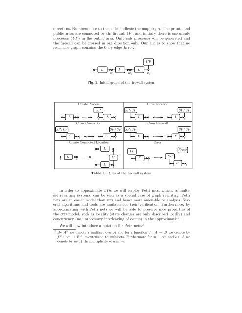
directions. Numbers close to the nodes indicate the mapping α. The private andpublic areas are connected by the firewall (F), and initially there is one unsafeprocesses (UP) in the public area. Only safe processes will be generated andthe firewall can be crossed in one direction only. Our aim is to show that noreachable graph contains the 0-ary edge Error.UPv 1Lw 1Fw 2Lv 2Fig. 1. Initial graph of the firewall system.Create ProcessSPSP/UPCross LocationSP/UPL1 2 1 2Cross ConnectionSP/UPSP/UPC1 2 1 2LLCCreate Connected LocationL1 2LC1 2LL1 2 1 2Cross FirewallSP/UPF1 2 1 2UPF1 2ErrorUPFFSP/UPError1 2Table 1. Rules of the firewall system.In order to approximate gtss we will employ Petri nets, which, as multisetrewriting systems, can be seen as a special case of graph rewriting. Petrinets are an easier model than gts and hence more amenable to analysis. Severalalgorithms and tools are available for their verification. Furthermore, byapproximating with Petri nets we will be able to preserve nice properties ofthe gts model, such as locality (state changes are only described locally) andconcurrency (no unnecessary interleaving of events) in the approximation.We will now introduce a notation for Petri nets. 22 By A ⊕ we denote a multiset over A and for a function f : A → B we denote byf ⊕ : A ⊕ → B ⊕ its extension to multisets. Furthermore for m ∈ A ⊕ and a ∈ A wedenote by m(a) the multiplicity of a in m.
Definition 4 (Petri net). Let ∆ be a finite set of labels. A ∆-labelled Petrinet is a tuple N = (S,T, • (),() • ,p), where S is the set of places, T is a set oftransitions, • (),() • : T → S ⊕ assign to each transition its pre-set and post-setand p : T → ∆ assigns a label to each transition. A marked Petri net is a pair(N,m N ), where N is a Petri net and m N ∈ S ⊕ is the initial marking.3 Approximated UnfoldingIn this section we will give a short overview of a technique that approximatesa graph transformation system by a structure that is both a Petri net and ahypergraph [3–5].First we define the notion of Petri graph which will be used to represent anover-approximation for a given gts. Note that the edges of the graph are at thesame time the places of the net and that the transitions are labelled with rulesof the gts.Definition 5 (Petri graph). Let G = (R,G 0 ) be a gts. A Petri graph (overR) is a tuple P = (G,N,µ), where G is a hypergraph, N = (E G ,T N , • (),() • ,p N )is an R-labelled Petri net where the places are the edges of G and µ associatesto each transition t ∈ T N , with p N (t) = (L,R,id), a hypergraph morphismµ(t) : L ∪ R → G such that • t = µ(t) ⊕ (E L ) and t • = µ(t) ⊕ (E R ).A Petri graph for the gts G is a pair (P,ι), where P = (G,N,µ) is a Petrigraph over R and ι : G 0 → G is a graph morphism. A marking is reachable(coverable) in Petri graph if it is reachable (coverable) in the underlying Petrinet with the multiset ι ⊕ (E G0 ) as the initial marking.We view Petri graphs as symbolic representations of transition systems withgraphs as states. Specifically each marking m of a Petri graph (G,N,m 0 ) canbe seen as representation of a graph, denoted by graph(m), according to thefollowing definition: We take the marked subgraph of G and duplicate each edgeas indicated by the marking.Alternatively one can define graph(m) as the unique graph H, up to isomorphism,such that H has no isolated nodes and there exists a morphismψ : H → G, injective on nodes, with ψ ⊕ (E H ) = m. Furthermore, wheneverthere exists a morphism ϕ : G ′ → G such that ϕ ⊕ (E G ′) ≤ m, then there existsan edge-injective morphism e m,ϕ :G ′ → graph(m) such that ψ ◦ e m,ϕ = ϕ.In order to obtain a Petri graph approximating a gts, we first need—asbuilding blocks—Petri graphs that describe the effect of a single rule.Definition 6 (Petri graph for a rewriting rule). Let r = (L,R,id) be arewriting rule. By P(t,r) = (G,N,µ) we denote a Petri graph with G = L∪R andN is a net with places S N = E L ∪ E R and one transition t such that p N (t) = r,• t = E L and t • = E R . Furthermore the morphism µ(t):L∪R → G is the identity.Given a gts G = (R,G 0 ) one can construct an over-approximating Petrigraph C G (also called the covering of G), using the following algorithm (see
Page 1 and 2: Counterexample-guided Abstraction R
Page 3: (edge-injective) whenever it is bij
Page 7 and 8: Cross FirewallErrorErrorF SP 2LCros
Page 9 and 10: 4.2 Relations on Nodes for Refining
Page 11 and 12: according to Definition 3 for each
Page 13 and 14: 5 Implementation and Experimental R
Page 15: References1. P.A. Abdulla, B. Jonss

Counterexample-guided Abstraction Refinement for the Analysis of ...

You also want an ePaper? Increase the reach of your titles

Delete template?

Save as template?